Defining Low-Dimensional Projections to Guide Protein Conformational Sampling

Abstract

Exploring the conformational space of proteins is critical to characterize their functions. Numerous methods have been proposed to sample a protein's conformational space, including techniques developed in the field of robotics and known as sampling-based motion-planning algorithms (or sampling-based planners). However, these algorithms suffer from the curse of dimensionality when applied to large proteins. Many sampling-based planners attempt to mitigate this issue by keeping track of sampling density to guide conformational sampling toward unexplored regions of the conformational space. This is often done using low-dimensional projections as an indirect way to reduce the dimensionality of the exploration problem. However, how to choose an appropriate projection and how much it influences the planner's performance are still poorly understood issues. In this article, we introduce two methodologies defining low-dimensional projections that can be used by sampling-based planners for protein conformational sampling. The first method leverages information about a protein's flexibility to construct projections that can efficiently guide conformational sampling, when expert knowledge is available. The second method builds similar projections automatically, without expert intervention. We evaluate the projections produced by both methodologies on two conformational search problems involving three middle-size proteins. Our experiments demonstrate that (i) defining projections based on expert knowledge can benefit conformational sampling and (ii) automatically constructing such projections is a reasonable alternative.

1. Introduction

Aprotein's activity is known to be characterized and modulated by its structure and the way it changes (Hegyi and Gerstein, 1999; Murphy, 2001). Understanding how a protein switches between conformations is essential to treat or prevent diseases related to the protein's dysfunction (Carlson, 2002). This requires gathering information about the protein's conformational space, that is, the space of all possible states of the protein (Hatfield and Lovas, 2014). Some information can be obtained experimentally (Schröder, 2015; van den Bedem and Fraser, 2015; Xu et al., 2015), but computational methods, such as molecular dynamics, are routinely involved in this process (Phillips et al., 2005; Seeliger and de Groot, 2009; Dror et al., 2012).

Initially developed in the field of robotics, sampling-based motion planning algorithms have been very successful at exploring a protein's conformational space [e.g., Al-Bluwi et al. (2012); Gipson et al. (2012)]. They have been applied in various studies to analyze protein loops (Cortés et al., 2004; Shehu and Kavraki, 2012), describe large-scale conformational changes (Raveh et al., 2009; Haspel et al., 2010; Luo and Haspel, 2013; Molloy and Shehu, 2015), model protein folding (Nath et al., 2012), or simulate protein–ligand unbinding (Devaurs et al., 2013). Their intrinsic principle is to randomly sample the conformational space (usually using a guiding heuristic) and build a graph over this space: nodes correspond to low-energy protein states and edges represent potential local transitions between them. This graph describes the topology of the underlying energy landscape and the connections between low-energy areas of the conformational space.

Among the numerous sampling-based planners, we focus on “expansive” planners (Hsu et al., 1999; Ladd and Kavraki, 2005; Şucan and Kavraki, 2010). They iteratively grow their graph by expanding it toward unexplored areas, which requires keeping track of conformational-space coverage. This is often done using low-dimensional projections, monitoring coverage of the projection space instead. Even though proteins comprise hundreds or thousands of degrees of freedom (DoFs), using dimensionality reduction techniques is justifiable: functionally relevant protein motions usually involve residues moving in a correlated manner, and can therefore be described with a few collective DoFs (Amadei et al., 1995; Teodoro et al., 2003).

Several approaches have been suggested to define low-dimensional projections that can guide conformational sampling. When specifically looking for a conformational pathway between two protein states, a simple one-dimensional projection can be defined using the distance to the goal state (Molloy and Shehu, 2015). When freely exploring conformational space, more sophisticated projections have been proposed, based on molecular energy (Olson et al., 2012) and structural properties of proteins described, for example, using contact matrices (Olson et al., 2012) or specific interatomic distances (Ballester and Richards, 2007; Shehu and Olson, 2010). However, there exists little work on analyzing whether such projections are beneficial (Olson et al., 2012). Interestingly, when using expansive planners, even randomly generated projections can be effective, at least for robotic articulated mechanisms (Şucan and Kavraki, 2009).

In this work, we focus on generating low-dimensional linear projections using some characterization of local protein flexibility, which relates to secondary structure. This is a common strategy, a typical instance being known as rigidity analysis, which has mostly been used to guide the conformational search locally (Thomas et al., 2007; Luo and Haspel, 2013). Here, in contrast, we define projections that can guide the search globally.

In this article, we propose a methodology leveraging expert knowledge about a protein's flexibility to construct projections that effectively guide the conformational sampling performed by expansive planners. These “expert” projections often perform better than randomly generated projections and “misguided” projections (designed in contradiction with the available flexibility information, for testing purposes). We also propose a technique to automatically build projections that are in essence similar to expert projections, but require no expert intervention. We show that these automatically built projections perform reasonably well and represent a useful alternative to expert projections.

This article is an extended version of Novinskaya et al. (2015). Our main additional contribution is the definition of automatically built projections. We also evaluate the impact of using different projections more thoroughly, by assessing conformational-space coverage, in addition to projection-space coverage.

2. Methods

2.1. Structured intuitive move selector

Our work builds on the Structured Intuitive Move Selector (SIMS) computational framework (Gipson et al., 2013), which allows exploring a protein's conformational space using robotics inspired sampling techniques. In SIMS, conformational sampling is restricted to using biophysically plausible perturbations of the protein's structure, referred to as “protein moves.” These are common perturbation strategies: loop sampling, rigid-body motion (fix one loop's end and move the other end), energy minimization, and random perturbations. To implement these moves and calculate molecular energy, SIMS relies on Rosetta (Das and Baker, 2008; Kaufmann et al., 2010).

SIMS involves an internal coordinate representation of proteins where bond lengths and bond angles are constant; peptide bond torsions are restricted to their trans conformation (i.e., \documentclass{aastex}\usepackage{amsbsy}\usepackage{amsfonts}\usepackage{amssymb}\usepackage{bm}\usepackage{mathrsfs}\usepackage{pifont}\usepackage{stmaryrd}\usepackage{textcomp}\usepackage{portland, xspace}\usepackage{amsmath, amsxtra}\pagestyle{empty}\DeclareMathSizes{10}{9}{7}{6}\begin{document} $$\omega { = 180^ \circ }$$ \end{document} ). Protein conformations are represented by vectors of backbone \documentclass{aastex}\usepackage{amsbsy}\usepackage{amsfonts}\usepackage{amssymb}\usepackage{bm}\usepackage{mathrsfs}\usepackage{pifont}\usepackage{stmaryrd}\usepackage{textcomp}\usepackage{portland, xspace}\usepackage{amsmath, amsxtra}\pagestyle{empty}\DeclareMathSizes{10}{9}{7}{6}\begin{document} $$( \varphi , { \kern 1pt} \psi )$$ \end{document} dihedral angles; therefore, a protein with \documentclass{aastex}\usepackage{amsbsy}\usepackage{amsfonts}\usepackage{amssymb}\usepackage{bm}\usepackage{mathrsfs}\usepackage{pifont}\usepackage{stmaryrd}\usepackage{textcomp}\usepackage{portland, xspace}\usepackage{amsmath, amsxtra}\pagestyle{empty}\DeclareMathSizes{10}{9}{7}{6}\begin{document} $$N + 1$$ \end{document} residues is modeled with \documentclass{aastex}\usepackage{amsbsy}\usepackage{amsfonts}\usepackage{amssymb}\usepackage{bm}\usepackage{mathrsfs}\usepackage{pifont}\usepackage{stmaryrd}\usepackage{textcomp}\usepackage{portland, xspace}\usepackage{amsmath, amsxtra}\pagestyle{empty}\DeclareMathSizes{10}{9}{7}{6}\begin{document} $$2N$$ \end{document} DoFs. Side chains are not modeled explicitly but optimized on-the-fly by Rosetta. This approach is similar in spirit to those involving coarse-grained potentials (Davtyan et al., 2012).

Proteins are decomposed into fragments (i.e., sets of residues) on which moves are applied. Fragments can be defined automatically, based on secondary structure, or by experts. Depending on how flexible parts of the protein are known to be (based on, e.g., rigidity analysis, B factors, and expert knowledge), fragments are assigned probabilities to be chosen during conformational sampling (Gipson et al., 2013).

In SIMS, the conformational search consists of incrementally building a tree in conformational space, starting from a known protein state. Tree nodes are conformations, and tree edges represent potential transitions between them. At each iteration of the SIMS algorithm, the tree is expanded by choosing a conformation in the tree (using some heuristic) and perturbing it with a move to produce a new conformation, which is added to the tree only if its energy is below a predefined threshold.

SIMS can be used in two different ways, performing directed searches or undirected searches in conformational space. A directed search aims at finding a sequence of conformations that can be seen as milestones along a transition between two known protein states; the term “directed” relates to the fact that these states are usually referred to as “start” and “goal.” An undirected search aims at covering large extents of the conformational space, starting from a given protein state, to obtain a good characterization of this space.

2.2. Sampling-based planners using projections

As already mentioned, in SIMS, a protein's conformational space is explored by building a tree of conformations over it (Gipson et al., 2013). Initially developed in the field of robotics, sampling-based motion planning algorithms can efficiently grow such a tree in a high-dimensional space. Among these sampling-based planners, expansive planners rely on maintaining sampling-density estimates to guide conformational sampling toward unexplored regions of the space (Hsu et al., 1999; Ladd and Kavraki, 2005; Şucan and Kavraki, 2010). This is often done using low-dimensional linear projections.

The projection space induced by a k-dimensional projection is discretized into a k-dimensional grid of equal-size cells. The expansive planner keeps track of conformational-space coverage indirectly by updating the number of conformations projected into every cell. At each iteration, to grow its tree, the planner chooses a cell based on probabilities determined by this coverage density, and picks the next conformation to be perturbed in this cell.

In this work, SIMS was evaluated with a recent expansive planner: Kinematic Planning by Interior-Exterior Cell Exploration (KPIECE) (Şucan and Kavraki, 2010). In KPIECE, a projection cell is chosen with probability strongly favoring exterior cells (i.e., cells having at least one empty neighbor cell) against interior cells (i.e., cells having no empty neighbor cell); then a conformation is picked with probability following a half-normal distribution favoring the most recently added conformations.

As mentioned earlier, protein conformations are represented by vectors of backbone \documentclass{aastex}\usepackage{amsbsy}\usepackage{amsfonts}\usepackage{amssymb}\usepackage{bm}\usepackage{mathrsfs}\usepackage{pifont}\usepackage{stmaryrd}\usepackage{textcomp}\usepackage{portland, xspace}\usepackage{amsmath, amsxtra}\pagestyle{empty}\DeclareMathSizes{10}{9}{7}{6}\begin{document} $$( \varphi , { \kern 1pt} \psi )$$ \end{document} dihedral angles. To linearly project a conformation, we first define a Euclidean embedding of the dihedral angles by constructing a vector of sines and cosines of these \documentclass{aastex}\usepackage{amsbsy}\usepackage{amsfonts}\usepackage{amssymb}\usepackage{bm}\usepackage{mathrsfs}\usepackage{pifont}\usepackage{stmaryrd}\usepackage{textcomp}\usepackage{portland, xspace}\usepackage{amsmath, amsxtra}\pagestyle{empty}\DeclareMathSizes{10}{9}{7}{6}\begin{document} $$( \varphi , { \kern 1pt} \psi )$$ \end{document} angles. A conformation for an \documentclass{aastex}\usepackage{amsbsy}\usepackage{amsfonts}\usepackage{amssymb}\usepackage{bm}\usepackage{mathrsfs}\usepackage{pifont}\usepackage{stmaryrd}\usepackage{textcomp}\usepackage{portland, xspace}\usepackage{amsmath, amsxtra}\pagestyle{empty}\DeclareMathSizes{10}{9}{7}{6}\begin{document} $$( N + 1 )$$ \end{document} -residue protein is thus represented by a \documentclass{aastex}\usepackage{amsbsy}\usepackage{amsfonts}\usepackage{amssymb}\usepackage{bm}\usepackage{mathrsfs}\usepackage{pifont}\usepackage{stmaryrd}\usepackage{textcomp}\usepackage{portland, xspace}\usepackage{amsmath, amsxtra}\pagestyle{empty}\DeclareMathSizes{10}{9}{7}{6}\begin{document} $$4N$$ \end{document} vector. This vector is projected into a k-dimensional subspace with a \documentclass{aastex}\usepackage{amsbsy}\usepackage{amsfonts}\usepackage{amssymb}\usepackage{bm}\usepackage{mathrsfs}\usepackage{pifont}\usepackage{stmaryrd}\usepackage{textcomp}\usepackage{portland, xspace}\usepackage{amsmath, amsxtra}\pagestyle{empty}\DeclareMathSizes{10}{9}{7}{6}\begin{document} $$k \times 4N$$ \end{document} matrix.

2.3. Low-dimensional linear projections

The justification for projecting high-dimensional spaces into lower dimensional spaces comes from the Johnson–Lindenstrauss theorem: distances between points in an n-dimensional space can be estimated with \documentclass{aastex}\usepackage{amsbsy}\usepackage{amsfonts}\usepackage{amssymb}\usepackage{bm}\usepackage{mathrsfs}\usepackage{pifont}\usepackage{stmaryrd}\usepackage{textcomp}\usepackage{portland, xspace}\usepackage{amsmath, amsxtra}\pagestyle{empty}\DeclareMathSizes{10}{9}{7}{6}\begin{document} $$1 + \varepsilon$$ \end{document} distortion by the distances between the corresponding points in a \documentclass{aastex}\usepackage{amsbsy}\usepackage{amsfonts}\usepackage{amssymb}\usepackage{bm}\usepackage{mathrsfs}\usepackage{pifont}\usepackage{stmaryrd}\usepackage{textcomp}\usepackage{portland, xspace}\usepackage{amsmath, amsxtra}\pagestyle{empty}\DeclareMathSizes{10}{9}{7}{6}\begin{document} $$\log ( n / { \varepsilon ^2} )$$ \end{document} -dimensional subspace (Johnson and Lindenstrauss, 1984). However, in protein modeling, projection dimensionality is much less than \documentclass{aastex}\usepackage{amsbsy}\usepackage{amsfonts}\usepackage{amssymb}\usepackage{bm}\usepackage{mathrsfs}\usepackage{pifont}\usepackage{stmaryrd}\usepackage{textcomp}\usepackage{portland, xspace}\usepackage{amsmath, amsxtra}\pagestyle{empty}\DeclareMathSizes{10}{9}{7}{6}\begin{document} $$\log ( N )$$ \end{document} : typically less than 10, often only 2 or 3. Such drastic dimensionality reduction remains reasonable because, even though proteins are extremely high-dimensional systems, few of their DoFs are usually involved in a specific large-scale motion (Amadei et al., 1995; Teodoro et al., 2003). Therefore, a projection based on these DoFs can benefit a conformational search aimed at modeling this motion.

We propose a methodology to define a projection matrix based on biological insights about a protein. Ideally, these insights should be provided by an expert with significant knowledge of the protein, such as, which protein regions are known to be flexible, to remain relatively unchanged, or to differ between distinct states. If no human expert can provide information, valuable insights can be derived from experimental studies analyzing protein dynamics, such as nuclear magnetic resonance spectroscopy (Ángyán and Gáspári, 2013) or hydrogen/deuterium exchange detected by mass spectrometry (Jaswal, 2013). If no experimental data is available, as a last resort, useful insights can be provided by computational studies, such as rigidity analysis (Fox et al., 2011) or normal mode analysis (Bakan et al., 2011). In all cases, we refer to these insights as “expert knowledge,” and to projections that leverage them as “expert projections.”

To construct expert projections, we analyze the expert knowledge to (i) identify the most flexible regions of the protein and (ii) predict how correlated they are. Indeed, flexible regions that might move in a correlated manner should be encoded together in one dimension; separate dimensions should correspond to independently moving regions. More specifically, each dimension should encode the list of residues comprised in its set of correlated flexible regions. Constructing a \documentclass{aastex}\usepackage{amsbsy}\usepackage{amsfonts}\usepackage{amssymb}\usepackage{bm}\usepackage{mathrsfs}\usepackage{pifont}\usepackage{stmaryrd}\usepackage{textcomp}\usepackage{portland, xspace}\usepackage{amsmath, amsxtra}\pagestyle{empty}\DeclareMathSizes{10}{9}{7}{6}\begin{document} $$k \times 4N$$ \end{document} projection matrix means defining k rows corresponding to the k dimensions of the projection space. Each row contains \documentclass{aastex}\usepackage{amsbsy}\usepackage{amsfonts}\usepackage{amssymb}\usepackage{bm}\usepackage{mathrsfs}\usepackage{pifont}\usepackage{stmaryrd}\usepackage{textcomp}\usepackage{portland, xspace}\usepackage{amsmath, amsxtra}\pagestyle{empty}\DeclareMathSizes{10}{9}{7}{6}\begin{document} $$4N$$ \end{document} values that are different from zero only in columns corresponding to the residues encoded in the corresponding dimension, knowing that each residue (except the first and last residues) is associated with four columns: \documentclass{aastex}\usepackage{amsbsy}\usepackage{amsfonts}\usepackage{amssymb}\usepackage{bm}\usepackage{mathrsfs}\usepackage{pifont}\usepackage{stmaryrd}\usepackage{textcomp}\usepackage{portland, xspace}\usepackage{amsmath, amsxtra}\pagestyle{empty}\DeclareMathSizes{10}{9}{7}{6}\begin{document} $$\{ \cos ( \varphi ) ,{ \kern 1pt} \, \sin ( \varphi ) ,{ \kern 1pt} \, \cos ( \psi ) ,{ \kern 1pt} \, \sin ( \psi ) \} $$ \end{document} . Note that each residue appears in only one row. Finally, rows are normalized to ensure matrix orthonormality, which is important to preserve distances.

By construction, an expert projection differs from a random projection in that it involves only selected residues; a random projection uses all residues, assigning them different weights. To ensure a comprehensive assessment of the expert projections, we also build “misguided projections” whose nature is similar to that of expert projections. In a misguided projection matrix, each row involves a few residues chosen within mostly rigid protein regions. Therefore, these projections are not expected to enhance conformational sampling.

2.4. Automatic construction of projections

Defining an expert projection can be a tedious process requiring significant knowledge of the studied protein. Therefore, we propose a methodology to automatically construct a projection matrix based on the protein's secondary structure and its decomposition into fragments, as defined in SIMS.

First, we rank fragments according to their weights, that is, their probabilities to be chosen for perturbation during conformational sampling. If two fragments have equal weights, we rank them based on their lengths: the longer a fragment, the greater its chances to be flexible. We want the automatically built projection to involve the fragments that will be the most “active” during conformational sampling.

To build the projection matrix, we assign the ranked fragments to different matrix rows. The first row contains only the top-ranked fragment, whose length is involved in defining the maximum number of residues than can be added to each remaining row. Then, we assign the next fragments to the next row, until the maximum number of residues is reached, and so on. We also make sure that each residue is included in only one row.

3. Experiments

Our objective is to investigate whether conformational sampling can be improved by using “good” low-dimensional projections. For that, we evaluate the expert projections, which take biological insights into account, and the automatically built projections, which are based on fragment decomposition. We compare them to randomly generated and misguided projections. Each experiment was run on a single thread of a quad-core 2.4 GHz Intel Xeon (Nahalem) CPU, with 24 hours time limit.

3.1. Studied proteins and associated projections

We report results obtained on three proteins that we selected because they have been extensively studied, both experimentally and computationally (Raveh et al., 2009; Gipson et al., 2013).

Cyanovirin-N (CVN) is a bacterial protein with 101 residues (Botos et al., 2002). It can adopt two stable states (PDB 2EZM and PDB 1L5E) that can be found together in solution. Switching between these states requires a large-scale domain swapping (the RMSD distance between them being around 17 Å), involving the correlated activity of three loop regions: residues 24–28, 50–55, and 75–80 (blue in Fig. 1a). Therefore, we generated a three-dimensional expert projection matrix, each row encoding one of these loops. The misguided projection also has three dimensions: two dimensions encode residues 40–45 and residues 83–88, respectively (orange in Fig. 1a), and the third dimension encompasses the remaining residues. Note that regions 40–45 and 83–88 correspond to middle parts of beta-strands with low flexibility. Finally, the projection that is automatically built by the method presented in Section 2.4 is the following: residues 75–79 are in the first dimension; residues 24–28 and 50–53 are in the second dimension; residues 15–16, 29–35, 39, 44–45, 57, and 65–67 are in the third dimension.

FIG. 1.

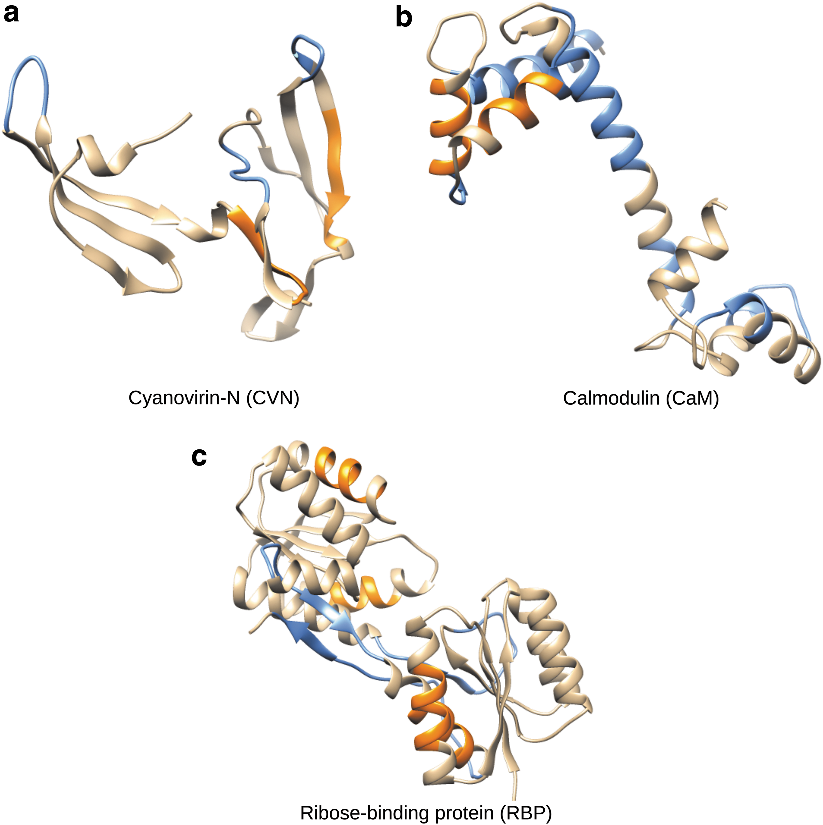
Proteins used in our experiments. Blue and orange areas indicate residues involved in expert and misguided projections, respectively.

Calmodulin (CaM) is a calcium-binding protein with 144 residues (Nelson and Chazin, 1998; Anthis et al., 2011). It has been observed in an open state (PDB 1CLL) and a closed state (PDB 1PRW) that are about 16 Å RMSD apart. The transition between them involves the unfolding of several helices and an hinge-like motion of the middle part of the central helix. We thus constructed a two-dimensional expert projection: the first dimension encodes the central hinge (residues 67–80), the second dimension includes other regions known to be involved in the transition (residues 5–20, 35–41, 52–57, 87–93, 107–116, and 126–129). These residues are in blue in Figure 1b. The misguided projection is also two-dimensional and includes residues of alpha helices not involved in the transition: both dimensions contain residues 30–35 and 47–52 (orange in Fig. 1b), but with different signs to ensure matrix orthonormality. Finally, the automatically built projection is defined as follows: residues 65–78 are in the first dimension, residues 53–59 and 124–132 are in the second dimension.

Ribose-binding protein (RBP) is the largest protein we studied, with 271 residues (Björkman et al., 1994; Björkman and Mowbray, 1998). It consists of two domains connected by three loops forming a hinge. The open conformation (PDB 2DRI) and the closed conformation (PDB 1URP) of RBP are only 4 Å RMSD apart, but the transition between them requires a correlated motion of the three loops (blue in Fig. 1c). We constructed a two-dimensional expert projection: the first dimension contains two of the loops (residues 91–104 and 226–237) and the second dimension contains the third loop (residues 253–269). The two-dimensional misguided projection is created using residues of several alpha helices: the first row includes residues 19–26 and 241–248 and the second row includes residues 140–147 and 168–175; these residues are in orange in Figure 1c. The automatically built projection is the following: residues 89–98 are in the first dimension and residues 64–69 and 253–259 are in the second dimension.

3.2. Improvement of directed search

In our first experiment, we evaluated the impact of the projections on the performance of a planner used for conformational sampling. For each protein and each type of projection, we performed 20 runs of a directed search between two protein states. We define the success rate of a projection as the percentage of runs that successfully produced a solution pathway within the 24 hours limit. Figure 2 shows that using the expert projection allows the planner to perform consistently and significantly better than when using the random or misguided projections. The success rate is more than doubled for CVN, and is about 1.5 times higher for CaM and RBP. The automatically built projection performs reasonably well: even though its success rate is lower than that of the expert projection, it is consistently better than those of the random and misguided projections.

FIG. 2.

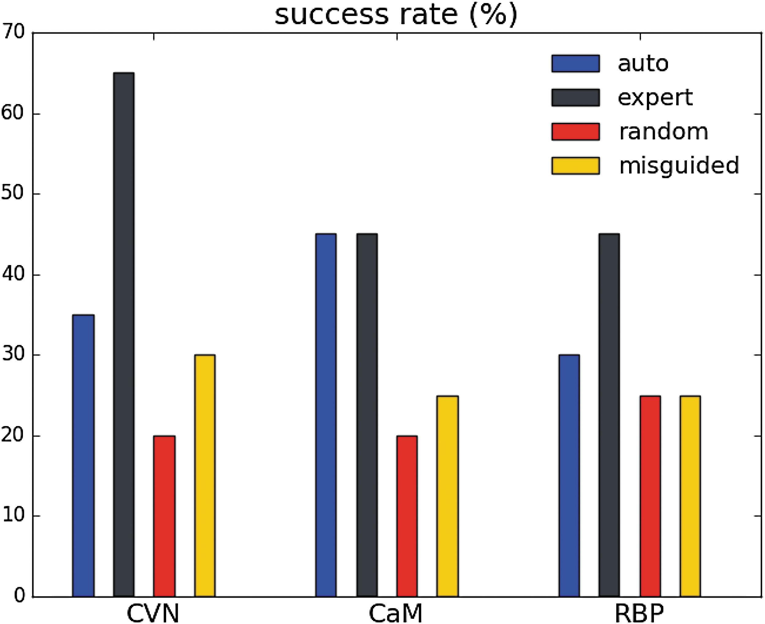
Success rates (i.e., percentage of successful runs, among 20) of the automatically generated, expert, randomly generated, and misguided projections, when performing directed searches between stable states of CVN, CaM, and RBP, with 24 hours time limit.

Another way to assess the projections is to plot their success rate as a function of the planner's running time (Fig. 3). The probabilities of success after 24 hours in this plot are the success rates reported in Figure 2. Plotting success rates over time allows for a richer comparison of the projections. First, Figure 3 shows that the previous observations about the expert and automatically built projections hold at any time for CVN. On the contrary, for RBP, the performance improvement achieved using the expert projection is observed only after some time. Finally, results for CaM illustrate that the automatically built projection can sometimes outperform the expert projection.

FIG. 3.

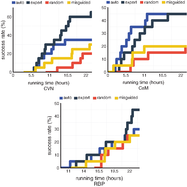
Success rates, as a function of the planner's running time, of the automatically generated, expert, randomly generated, and misguided projections, when performing directed searches between stable states of CVN, CaM, and RBP.

As the expert and automatically built projections were specifically conceived to enhance the directed search, it is reassuring to observe such performance improvement. However, the improvement is sometimes small, highlighting the difficulty of defining a projection that would consistently be beneficial, even for a single task. Next, we examine how the projections impact another task.

3.3. Improvement of undirected search

In a second experiment, we evaluated the extent of the conformational exploration performed by a planner using various projections. For each protein and each projection type, we performed 20 runs of an undirected search starting from a given state.

3.3.1. Projection-space coverage

One way to quantify the extent of conformational exploration, at least indirectly, is to assess the volume of projection space that is explored. For that, we count the number of cells containing the projection of at least one conformation (i.e., nonempty cells). The number of explored cells is averaged over 20 runs, for each protein and each projection type (Fig. 4). Clearly, the automatically built projection consistently and significantly outperforms the others: it yields number of explored cells at least four times higher. The expert projection performs better than the random and misguided projections only for CVN; for CaM and RBP, it outperforms only the misguided projection.

FIG. 4.

Box plots representing the average number of cells in projection space explored by the planner (over 20 runs) when performing 24 hours-long undirected searches for CVN, CaM, and RBP, using the automatically generated, expert, randomly generated, and misguided projections.

3.3.2. Conformational-space coverage

A better way to assess the extent of conformational exploration is to estimate the volume of explored conformational space itself (Yang et al., 2014; Cazals et al., 2015). For that, we count the number of \documentclass{aastex}\usepackage{amsbsy}\usepackage{amsfonts}\usepackage{amssymb}\usepackage{bm}\usepackage{mathrsfs}\usepackage{pifont}\usepackage{stmaryrd}\usepackage{textcomp}\usepackage{portland, xspace}\usepackage{amsmath, amsxtra}\pagestyle{empty}\DeclareMathSizes{10}{9}{7}{6}\begin{document} $$2N$$ \end{document} -dimensional balls of radius 1 Å needed to cover the set of conformations sampled by the planner. After the planner has stopped, we use a simple greedy method to cover the sampled conformations with such balls. We repeat the following until they are all covered: randomly pick an uncovered conformation and make it the center of a new ball and mark as covered all the conformations within this ball. Despite producing random coverages and not optimal coverages, this method yields ball counts whose standard deviation is usually less than 1%. Therefore, it provides good estimates of conformational-space coverage.

The number of balls covering the sampled conformations is averaged over 20 runs, for each protein and each projection type. Figure 5 shows that mixed results were obtained. Neither the expert nor the automatically built projections outperform the random or misguided projections. Which projection performs best depends on the studied protein. A reassuring result is that the expert projection is never the worst projection. However, the inconsistency of the automatically built projection highlights its lack of generality. The differences between Figures 4 and 5 also illustrate that a good projection-space coverage does not necessarily translate into a good conformational-space coverage.

FIG. 5.

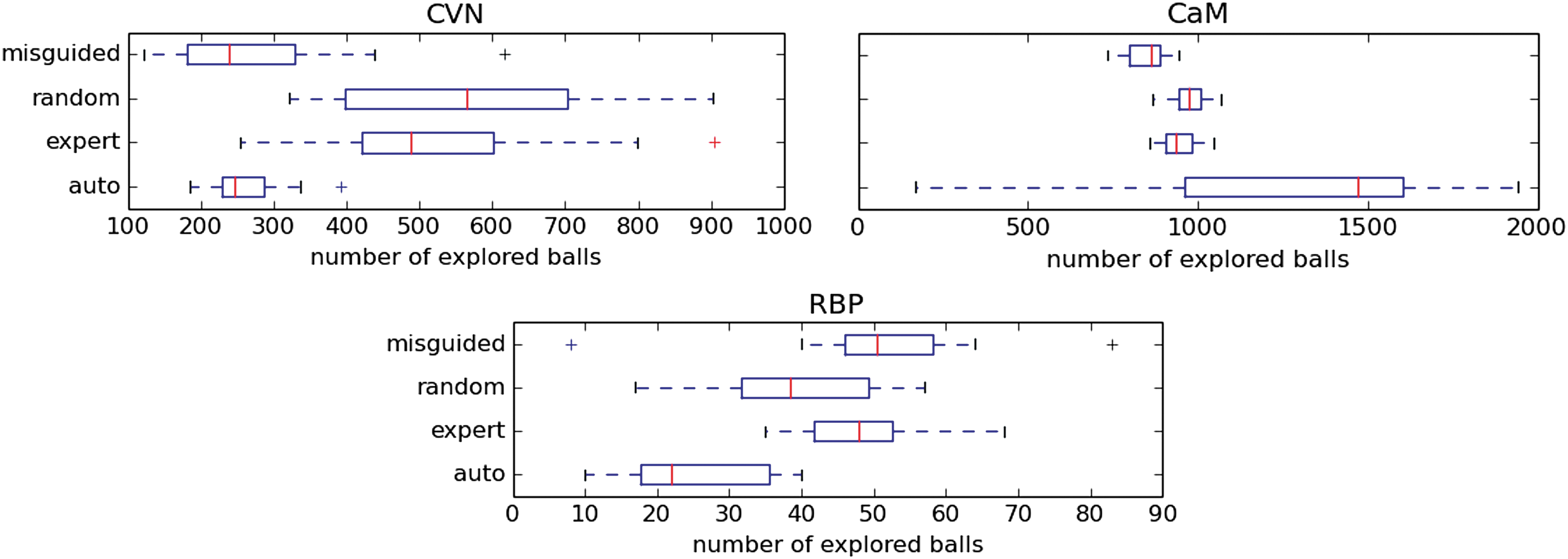
Box plots representing the average number of balls (in conformational space) required to cover the set of conformations sampled by the planner (over 20 runs) when performing 24 hours-long undirected searches for CVN, CaM, and RBP, using the automatically generated, expert, randomly generated, and misguided projections.

3.3.3. Discussion

The fact that a given projection increases projection-space coverage only means that this projection is well aligned with some flexible parts of the protein; in this case, the planner is fully able to exploit this projection as an expansion heuristic. However, this does not necessarily translate into an overall increase of conformational-space coverage, which could be achieved only by having a projection better capturing the overall protein flexibility. Our experiment shows that it is also a task-specific issue, and that defining a projection that would perform well across a wide range of tasks could be challenging.

4. Conclusion

In this article, through our experiments with the SIMS framework, using the KPIECE expansive planner, we have shown that protein conformational sampling performed by sampling-based planners can be improved using relevant low-dimensional linear projections. Our contribution consists in proposing two methods to define such projections. First, using expert knowledge about a protein's flexibility, we can define expert projections that efficiently guide conformational sampling. Second, even without any expert intervention, it is possible to automatically build projections that perform reasonably well. These two methods were conceived with a directed search in mind, and therefore benefit mostly this task. The mixed but promising results obtained with the undirected search highlight the difficulty of defining projections that could benefit any task.

As part of our future work, we plan to investigate whether projections should remain task-specific, or whether it is possible to define efficient generic projections. In addition, we want to develop other methods to automatically generate (possibly nonlinear) projections, using normal mode analysis, principal component analysis, and graph-theory-based rigidity analysis. It would be interesting to assess how a projection is performing and to modify it, during the conformational exploration. We also plan to analyze the influence of dimensionality on the performance of these projections and to study multichain proteins.

Footnotes

Acknowledgments

This work was supported, in part, by the National Science Foundation (under Grant ABI 0960612 and Grant CCF 1423304) and by Rice University Funds. Experiments were run on equipment that was supported, in part, by the Data Analysis and Visualization Cyberinfrastructure funded by NSF under Grant OCI 0959097, as well as on equipment that was supported by the Cyberinfrastructure for Computational Research funded by NSF under Grant CNS 0821727.

Author Disclosure Statement

No competing financial interests exist.

References

Al-Bluwi

, Siméon

, and Cortés

2012. Motion planning algorithms for molecular simulations: A survey. Comput. Sci. Rev., 6, 125–143.

Amadei

, Linssen

A.B.

, De Groot

B.L.

, et al. 1995. Essential degrees of freedom of proteins. Mol. Eng., 5, 71–79.

Ángyán

A.F.

, and Gáspári

2013. Ensemble-based interpretations of NMR structural data to describe protein internal dynamics. Molecules, 18, 10548–10567.

Anthis

N.J.

, Doucleff

, and Clore

G.M.

2011. Transient, sparsely populated compact states of Apo and calcium-loaded Calmodulin probed by paramagnetic relaxation enhancement: Interplay of conformational selection and induced fit. J. Am. Chem. Soc., 133, 18966–18974.

Bakan

, Meireles

L.M.

, and Bahar

2011. ProDy: Protein dynamics inferred from theory and experiments. Bioinformatics, 27, 1575–1577.

Ballester

P.J.

, and Richards

W.G.

2007. Ultrafast shape recognition to search compound databases for similar molecular shapes. J. Comput. Chem., 28, 1711–1723.

Björkman

A.J.

, Binnie

R.A.

, Zhang

, et al. 1994. Probing protein-protein interactions. The ribose-binding protein in bacterial transport and chemotaxis. J. Biol. Chem., 269, 30206–30211.

Björkman

A.J.

, and Mowbray

S.L.

1998. Multiple open forms of ribose-binding protein trace the path of its conformational change. J. Mol. Biol., 279, 651–664.

Botos

, O'Keefe

B.R.

, Shenoy

S.R.

, et al. 2002. Structures of the complexes of a potent anti-HIV protein Cyanovirin-N and high mannose oligosaccharides. J. Biol. Chem., 277, 34336–34342.

10.

Carlson

H.A.

2002. Protein flexibility is an important component of structure-based drug discovery. Curr. Pharm. Des., 8, 1571–1578.

11.

Cazals

, Dreyfus

, Mazauric

, et al. 2015. Conformational ensembles and sampled energy landscapes: Analysis and comparison. J. Comput. Chem., 36, 1213–1231.

12.

Cortés

, Siméon

, Remaud-Siméon

, et al. 2004. Geometric algorithms for the conformational analysis of long protein loops. J. Comput. Chem., 25, 956–967.

13.

Das

, and Baker

2008. Macromolecular modeling with Rosetta. Annu. Rev. Biochem., 77, 363–382.

14.

Davtyan

, Schafer

N.P.

, Zheng

, et al. 2012. AWSEM-MD: Protein structure prediction using coarse-grained physical potentials and bioinformatically based local structure biasing. J. Phys. Chem. B, 116, 8494–8503.

15.

Devaurs

, Bouard

, Vaisset

, et al. 2013. MoMA-LigPath: A web server to simulate protein-ligand unbinding. Nucl. Acids Res., 41, W297–W302.

16.

Dror

R.O.

, Dirks

R.M.

, Grossman

J.P.

, et al. 2012. Biomolecular simulation: A computational microscope for molecular biology. Annu. Rev. Biophys., 41:429–452.

17.

Fox

, Jagodzinski

, Li

, et al. 2011. KINARI-Web: A server for protein rigidity analysis. Nucl. Acids Res., 39(suppl 2):W177–W183.

18.

Gipson

, Hsu

, Kavraki

L.E.

, et al. 2012. Computational models of protein kinematics and dynamics: Beyond simulation. Annu. Rev. Anal. Chem., 5:273–291.

19.

Gipson

, Moll

, and Kavraki

L.E.

2013. SIMS: A hybrid method for rapid conformational analysis. PLoS One. 8, e68826.

20.

Haspel

, Moll

, Baker

M.L.

, et al. 2010. Tracing conformational changes in proteins. BMC Struct. Biol., 10(Suppl 1):S1.

21.

Hatfield

M.P.

, and Lovas

2014. Conformational sampling techniques. Curr. Pharm. Des., 20, 3303–3313.

22.

Hegyi

, and Gerstein

1999. The relationship between protein structure and function: A comprehensive survey with application to the yeast genome. J. Mol. Biol., 288, 147–164.

23.

Hsu

, Latombe

J.-C.

, and Motwani

1999. Path planning in expansive configuration spaces. Int. J. Comput. Geom. Appl., 9, 495–512.

24.

Jaswal

S.S.

2013. Biological insights from hydrogen exchange mass spectrometry. Biochim. Biophys. Acta, 1834, 1188–1201.

25.

Johnson

W.B.

, and Lindenstrauss

1984. Extensions of Lipschitz mappings into a Hilbert space. Contemp. Math., 26:189–206.

26.

Kaufmann

K.W.

, Lemmon

G.H.

, DeLuca

S.L.

, et al. 2010. Practically useful: What the Rosetta protein modeling suite can do for you. Biochemistry, 49, 2987–2998.

27.

Ladd

A.M.

, and Kavraki

L.E.

2005. Fast tree-based exploration of state space for robots with dynamics, 297–312. In Erdmann

, Overmars

, Hsu

, and van der Stappen

, eds. Algorithmic Foundations of Robotics VI, volume 17 of Springer Tracts in Advanced Robotics. Springer, Berlin; Heidelberg.

28.

Luo

, and Haspel

2013. Multi-resolution rigidity-based sampling of protein conformational paths. In Proceedings of the ACM-BCB, 786–792. ACM, New York.

29.

Molloy

, and Shehu

2015. Interleaving global and local search for protein motion computation, 175–186. In Harrison

, Li

, and Măndoiu

, eds. Bioinformatics Research and Applications, volume 9096 of Lecture Notes in Computer Science. Springer International publishing, Switzerland.

30.

Murphy

K.P.

, ed. 2001. Protein Structure, Stability, and Folding, volume 168 of Methods in Molecular Biology. Humana Press, New York City.

31.

Nath

, Thomas

, Ekenna

, et al. 2012. A multi-directional rapidly exploring random graph (mRRG) for protein folding. In Proceedings of the ACM-BCB, 44–51. ACM, New York.

32.

Nelson

M.R.

, and Chazin

W.J.

1998. An interaction-based analysis of calcium-induced conformational changes in

\documentclass{aastex}\usepackage{amsbsy}\usepackage{amsfonts}\usepackage{amssymb}\usepackage{bm}\usepackage{mathrsfs}\usepackage{pifont}\usepackage{stmaryrd}\usepackage{textcomp}\usepackage{portland, xspace}\usepackage{amsmath, amsxtra}\pagestyle{empty}\DeclareMathSizes{10}{9}{7}{6}\begin{document}$${ \rm{C}}{{ \rm{a}}^{{ \rm{2}} + }}$$\end{document}

sensor proteins. Protein Sci. 7, 270–282.

33.

Novinskaya

, Devaurs

, Moll

, et al. 2015. Improving protein conformational sampling by using guiding projections. In Proceedings of the Computational Structural Bioinformatics Workshop (BIBM’15). IEEE, New York.

34.

Olson

, Molloy

, Hendi

S.F.

, et al. 2012. Guiding probabilistic search of the protein conformational space with structural profiles. J. Bioinform. Comput. Biol. 10, 1242005.

35.

Phillips

J.C.

, Braun

, Wang

, et al. 2005. Scalable molecular dynamics with NAMD. J. Comput. Chem., 26, 1781–1802.

36.

Raveh

, Enosh

, Schueler-Furman

, et al. 2009. Rapid sampling of molecular motions with prior information constraints. PLoS Comput. Biol. 5, e1000295.

37.

Schröder

G.F.

2015. Hybrid methods for macromolecular structure determination: Experiment with expectations. Curr. Opin. Struct. Biol., 31:20–27.

38.

Seeliger

, and de Groot

B.L.

2009. tCONCOORD-GUI: Visually supported conformational sampling of bioactive molecules. J. Comput. Chem., 30, 1160–1166.

39.

Shehu

, and Kavraki

L.E.

2012. Modeling structures and motions of loops in protein molecules. Entropy, 14, 252–290.

40.

Shehu

, and Olson

2010. Guiding the search for native-like protein conformations with an ab-initio tree-based exploration. Int. J. Robot. Res., 29, 1106–1127.

41.

Şucan

I.A.

, and Kavraki

L.E.

2009. n the performance of random linear projections for sampling-based motion planning. In Proceedings of the IEEE/RSJ IROS, 2434–2439. IEEE, New York.

42.

Şucan

I.A.

, and Kavraki

L.E.

2010. Kinodynamic motion planning by interior-exterior cell exploration, 449–464. In Algorithmic Foundations of Robotics VIII. Chirikjian

, Chaset

, Morales

, and Murphey

, eds. Springer-Verlag, Berlin; Heidelberg. Springer-Verlag.

43.

Teodoro

M.L.

, Phillips

G.N.

Jr , and Kavraki

L.E.

2003. Understanding protein flexibility through dimensionality reduction. J. Comput. Biol., 10, 617–634.

44.

Thomas

, Tang

, Tapia

, et al. 2007. Simulating protein motions with rigidity analysis. J. Comput. Biol., 14, 839–855.

45.

van den Bedem

, and Fraser

J.S

. 2015. Integrative, dynamic structural biology at atomic resolution—It's about time. Nat. Methods, 12, 307–318.

46.

, Yan

, Wohlhueter

, et al. 2015. Integrative modeling of macromolecular assemblies from low to near-atomic resolution. Comput. Struct. Biotechnol. J., 13:492–503.

47.

Yang

, Salmon

, and Al-Hashimi

H.M.

2014. Measuring similarity between dynamic ensembles of biomolecules. Nat. Meth., 11, 552–554.