Flexible Modeling of Genetic Effects on Function-Valued Traits

Abstract

Genome-wide association studies commonly examine one trait at a time. Occasionally they examine several related traits with the hope of increasing power; in such a setting, the traits are not generally smoothly varying in any way such as time or space. However, for function-valued traits, the trait is often smoothly varying along the axis of interest, such as space or time. For instance, in the case of longitudinal traits such as growth curves, the axis of interest is time; for spatially varying traits such as chromatin accessibility, it would be position along the genome. Although there have been efforts to perform genome-wide association studies with such function-valued traits, the statistical approaches developed for this purpose often have limitations such as requiring the trait to behave linearly in time or space, or constraining the genetic effect itself to be constant or linear in time. Herein, we present a flexible model for this problem—the Partitioned Gaussian Process—which removes many such limitations and is especially effective as the number of time points increases. The theoretical basis of this model provides machinery for handling missing and unaligned function values such as would occur when not all individuals are measured at the same time points. Furthermore, we make use of algebraic refactorizations to substantially reduce the time complexity of our model beyond the naive implementation. Finally, we apply our approach and several others to synthetic data before closing, with some directions for improved modeling and statistical testing.

1. Introduction

Genome-wide association studies (GWAS) commonly examine one trait at a time. Occasionally they examine several related traits with the hope of increasing power; in such a setting, the traits are not generally smoothly varying in any way such as time or space. However, with the advent of wearables for health and the “quantified self” movement, the broad deployment of cheap sensors in domains such as agriculture and breeding, and the approaching ubiquity of electronic health records, we shall soon see the ubiquity of function-valued traits. Longitudinal traits are one example of function-valued traits—traits that can be viewed as a smooth function of some variable. For example, that variable could be time in a clinical history corresponding to a longitudinal trait, or it could be position in the genome, corresponding to a spatial trait such as chromatin accessibility (Shim and Stephens, 2015). Such function-valued traits offer new opportunities to dissect genetics. However, maximally benefiting from such opportunities requires that the rich, smoothly varying structure within these traits can be leveraged by the statistical model of choice.

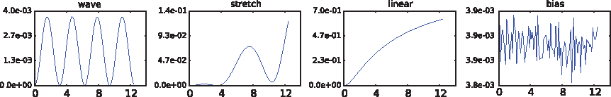
Rich trait structure arises from constraints in the physical world such as that time moves forward and is smoothly varying, or that the correlation between positions on the genome is slowly decreasing according to genetic distance on the chromosome. Modeling approaches in these settings should take into account such constraints while still allowing for flexibility in the shapes of the traits. Furthermore, it stands to reason that the genetic effect might alter the functional form of a trait, such as the shape of a growth curve, a pattern of weight gain, bone loss, or electrocardiogram signal. Thus, flexible modeling beyond linear genetic effects is also one of our goals. Figure 1 shows a set of simple canonical traits and genetic effects that we would like to be able to detect. These canonical traits will also serve as the basis of our synthetic experiments for comparing the behavior of several modeling approaches. In these examples, by design, a genetic effect that is constant or linear in time will fail to properly model the data. Although these traits are rather idealized, they present a good starting point with which to examine the problem.

FIG. 1.

Simulated traits with 100 time points taking on values uniformly spaced between 0 and 12. Each plot shows what the mean (noise-free) trait looks like for each of the SNP values 0 (blue), 1 (green), and 2 (red). The noise added (not shown) is iid with respect to both time and individuals. Note that we here display the maximum genetic effect for each kind of trait for visual clarity. SNP, single-nucleotide polymorphism.

The simplest problem we might tackle in our chosen setting is to find out which individual single-nucleotide polymorphisms (SNPs) are correlated to the trait of interest, a so-called marginal test. Those that are correlated are then assumed to have a reasonable probability of being causal for the trait, or of tagging a nearby SNP that is causal for the trait. Although it is also of interest to test sets of SNPs jointly (Wu et al., 2010; Listgarten et al., 2013; He et al., 2015), we here focus on marginal SNP testing, leaving a generalization to set tests for future work. The solution to this marginal testing problem entails (1) proposing a statistical model of the data and (2) obtaining some weight of evidence of a genetic effect such as a p value or Bayes factor. In this work, we focus primarily on the first task, but discuss our future directions for the second task in concluding.

Numerous approaches for analyzing function-valued genetic associations have been proposed in recent years (Zhang, 1997; Kendziorski et al., 2002; Smith et al., 2010; Das et al., 2011; Furlotte et al., 2012; Wang, 2012; Chung and Zou, 2014; Ding et al., 2014; Musolf et al., 2014; He et al., 2015; Jaffa et al., 2015; Shim and Stephens, 2015; Sikorska et al., 2015). However, these do not necessarily make effective use of the rich trait structure to increase power because they often assume restrictive forms of the genetic effect or the trait itself. Also, in some cases, the statistical efficiency does not scale well with the number of time points, which are expected to be quite numerous in the settings discussed earlier. Next we give a brief overview of some of these approaches and their weaknesses in tackling the kinds of problems we are interested in.

Sikorska et al. use an approximate linear mixed model that accounts for correlation in time and assumes that a trait evolves over time in a linear manner; they also assume that the SNP effect itself is additive. Musolf et al. first cluster the trait without accounting for genetics and then seek genetic effects on the cluster labels, thereby presupposing that all causal SNPs segregate the traits in a similar manner. Shim et al. first apply a wavelet transform to the trait data, thereby transforming the traits to lie in a coordinate system based on (hierarchical) scales and locations; they then perform association testing in this new space. Although this approach enables flexible functions of time to be modeled, the SNP effects are restricted to be linear because the wavelet transform itself is linear. Das et al. construct a different Legendre polynomial-based model to model the trait for each test SNP allele, learning each model in a largely independent manner. They then test whether the time-specific mean effects are different between the alleles, although it is not clear how they combine time points in their statistical testing framework. Also note that Das et al. remove SNPs with minor allele frequency (MAF) less than 10% from their experiments because the MAF dictates the amount of data available to each allele-specific model. Finally, there has been some related work on detecting differential expression using Gaussian process (GP) regression that shares many aspects of our approach, while differing in several respects, including parameter sharing, independence among individuals, and substantial differences in time complexity in the case of aligned time points, partly owing to the use of a different noise model and inference algorithm (Stegle et al., 2010).

In our work, we propose an extremely flexible approach for modeling function-valued traits with genetic effects. In particular, our approach, based on GP regression with a radial basis function (RBF) kernel (Rasmussen and Williams, 2005) at its core, can in principle capture any smoothly varying trait in time, where the smoothness is controlled by a “length scale” parameter. This length scale parameter is estimated using maximum likelihood, thereby effectively deducing the complexity of the trait functional form directly from the data. As for the genetic effect, similarly to Das et al., our model has three components corresponding to three partitions of the data, yielding an extremely nonrestrictive class of genetic effects because the GP for each allele can look completely different from the other alleles when no parameters are shared. In our experiments, we assume that basic properties such as the noise level and length scale are likely to be common to all alleles and hence tie these parameters together for more efficient statistical estimation. However, the model need not be used in this manner. Furthermore, because the RBF kernel effectively integrates out the time points, the number of model parameters does not scale with the number of time points, but is instead fixed—a desirable property when many time points are observed. We call our model the Partitioned GP for partitioned GP regression.

2. Partitioned Gaussian Processes

As already mentioned, our model uses at its core GP regression (Rasmussen and Williams, 2005), a class of models that encompasses linear mixed models, the more widely used concept in genetics (Yu et al., 2006; Kang et al., 2008; Listgarten et al., 2010; Lippert et al., 2011). The GP regression literature contains results not typically found in the genetics community that we make use of, including the use of RBF kernels and Kronecker product-based refactorizations of matrix-variate normal probability distributions, yielding computational efficiencies (Stegle et al., 2011) in the case of aligned and nonmissing time points. Also, although we have not yet implemented it, by virtue of using the GP machinery, we can immediately access variational approximations to reduce computational time complexity (Quiñonero Candela and Rasmussen, 2005; Titsias, 2009) in the case of missing data or unaligned time points. We now formally introduce our null model, followed by an exposition of how to do efficient computations in it before introducing the alternative model and computation of p values.

2.1. Null model

Our null model, M₀, assumes that the SNP has no effect on the trait (and so does not enter the model), but does capture correlation in time by way of an RBF kernel. Let Y be the \documentclass{aastex}\usepackage{amsbsy}\usepackage{amsfonts}\usepackage{amssymb}\usepackage{bm}\usepackage{mathrsfs}\usepackage{pifont}\usepackage{stmaryrd}\usepackage{textcomp}\usepackage{portland, xspace}\usepackage{amsmath, amsxtra}\pagestyle{empty}\DeclareMathSizes{10}{9}{7}{6}\begin{document} $$N \times T$$ \end{document} matrix of traits for N individuals and T time points. Let W be the \documentclass{aastex}\usepackage{amsbsy}\usepackage{amsfonts}\usepackage{amssymb}\usepackage{bm}\usepackage{mathrsfs}\usepackage{pifont}\usepackage{stmaryrd}\usepackage{textcomp}\usepackage{portland, xspace}\usepackage{amsmath, amsxtra}\pagestyle{empty}\DeclareMathSizes{10}{9}{7}{6}\begin{document} $$N \times T$$ \end{document} times at which the traits were measured, and let \documentclass{aastex}\usepackage{amsbsy}\usepackage{amsfonts}\usepackage{amssymb}\usepackage{bm}\usepackage{mathrsfs}\usepackage{pifont}\usepackage{stmaryrd}\usepackage{textcomp}\usepackage{portland, xspace}\usepackage{amsmath, amsxtra}\pagestyle{empty}\DeclareMathSizes{10}{9}{7}{6}\begin{document} $${ \rm{vec}} ( {\bf Y} )$$ \end{document} denote the unrolled version of Y into a vector of dimension \documentclass{aastex}\usepackage{amsbsy}\usepackage{amsfonts}\usepackage{amssymb}\usepackage{bm}\usepackage{mathrsfs}\usepackage{pifont}\usepackage{stmaryrd}\usepackage{textcomp}\usepackage{portland, xspace}\usepackage{amsmath, amsxtra}\pagestyle{empty}\DeclareMathSizes{10}{9}{7}{6}\begin{document} $$NT \times 1$$ \end{document} , \documentclass{aastex}\usepackage{amsbsy}\usepackage{amsfonts}\usepackage{amssymb}\usepackage{bm}\usepackage{mathrsfs}\usepackage{pifont}\usepackage{stmaryrd}\usepackage{textcomp}\usepackage{portland, xspace}\usepackage{amsmath, amsxtra}\pagestyle{empty}\DeclareMathSizes{10}{9}{7}{6}\begin{document} \begin{align*} { \rm{vec}} ( { \bf Y} ) = \left( { \begin{matrix} {{y_{11}}} \\ {{y_{21}}} \\ \vdots \\ {{y_{NT}}} \\ \end{matrix} } \right). \end{align*} \end{document}

Then \documentclass{aastex}\usepackage{amsbsy}\usepackage{amsfonts}\usepackage{amssymb}\usepackage{bm}\usepackage{mathrsfs}\usepackage{pifont}\usepackage{stmaryrd}\usepackage{textcomp}\usepackage{portland, xspace}\usepackage{amsmath, amsxtra}\pagestyle{empty}\DeclareMathSizes{10}{9}{7}{6}\begin{document} \begin{align*} {M_0}:p ( { \rm{vec}} ( { \bf Y} ) ) = { \mathcal N} \left( {{ \rm{vec}} ( { \bf Y} ) { \kern 1pt} \vert { \kern 1pt} { \bf 0} , \sigma _r^2{{ \bf K}_{RBF}} ( { \bf W , W \vert }l ) + \sigma _e^2{{\bf I}_{NT}}} \right) , \tag{1} \end{align*} \end{document}

where \documentclass{aastex}\usepackage{amsbsy}\usepackage{amsfonts}\usepackage{amssymb}\usepackage{bm}\usepackage{mathrsfs}\usepackage{pifont}\usepackage{stmaryrd}\usepackage{textcomp}\usepackage{portland, xspace}\usepackage{amsmath, amsxtra}\pagestyle{empty}\DeclareMathSizes{10}{9}{7}{6}\begin{document} $${ \mathcal N} \left( {a{ \kern 1pt} \vert { \kern 1pt} b , { \bf C}} \right)$$ \end{document} is a Gaussian distribution in vector a with mean b and covariance C, \documentclass{aastex}\usepackage{amsbsy}\usepackage{amsfonts}\usepackage{amssymb}\usepackage{bm}\usepackage{mathrsfs}\usepackage{pifont}\usepackage{stmaryrd}\usepackage{textcomp}\usepackage{portland, xspace}\usepackage{amsmath, amsxtra}\pagestyle{empty}\DeclareMathSizes{10}{9}{7}{6}\begin{document} $${{ \bf I}_{NT}}$$ \end{document} is the \documentclass{aastex}\usepackage{amsbsy}\usepackage{amsfonts}\usepackage{amssymb}\usepackage{bm}\usepackage{mathrsfs}\usepackage{pifont}\usepackage{stmaryrd}\usepackage{textcomp}\usepackage{portland, xspace}\usepackage{amsmath, amsxtra}\pagestyle{empty}\DeclareMathSizes{10}{9}{7}{6}\begin{document} $$NT \times NT$$ \end{document} identity matrix, \documentclass{aastex}\usepackage{amsbsy}\usepackage{amsfonts}\usepackage{amssymb}\usepackage{bm}\usepackage{mathrsfs}\usepackage{pifont}\usepackage{stmaryrd}\usepackage{textcomp}\usepackage{portland, xspace}\usepackage{amsmath, amsxtra}\pagestyle{empty}\DeclareMathSizes{10}{9}{7}{6}\begin{document} $$\sigma _r^2$$ \end{document} and \documentclass{aastex}\usepackage{amsbsy}\usepackage{amsfonts}\usepackage{amssymb}\usepackage{bm}\usepackage{mathrsfs}\usepackage{pifont}\usepackage{stmaryrd}\usepackage{textcomp}\usepackage{portland, xspace}\usepackage{amsmath, amsxtra}\pagestyle{empty}\DeclareMathSizes{10}{9}{7}{6}\begin{document} $$\sigma _e^2$$ \end{document} are scalar parameters that control the overall variance contributed by each kernel, and \documentclass{aastex}\usepackage{amsbsy}\usepackage{amsfonts}\usepackage{amssymb}\usepackage{bm}\usepackage{mathrsfs}\usepackage{pifont}\usepackage{stmaryrd}\usepackage{textcomp}\usepackage{portland, xspace}\usepackage{amsmath, amsxtra}\pagestyle{empty}\DeclareMathSizes{10}{9}{7}{6}\begin{document} $${{ \bf K}_{RBF}} ( l )$$ \end{document} is an \documentclass{aastex}\usepackage{amsbsy}\usepackage{amsfonts}\usepackage{amssymb}\usepackage{bm}\usepackage{mathrsfs}\usepackage{pifont}\usepackage{stmaryrd}\usepackage{textcomp}\usepackage{portland, xspace}\usepackage{amsmath, amsxtra}\pagestyle{empty}\DeclareMathSizes{10}{9}{7}{6}\begin{document} $$NT \times NT$$ \end{document} RBF kernel with length scale parameter l and elements defined by \documentclass{aastex}\usepackage{amsbsy}\usepackage{amsfonts}\usepackage{amssymb}\usepackage{bm}\usepackage{mathrsfs}\usepackage{pifont}\usepackage{stmaryrd}\usepackage{textcomp}\usepackage{portland, xspace}\usepackage{amsmath, amsxtra}\pagestyle{empty}\DeclareMathSizes{10}{9}{7}{6}\begin{document} $$ { K_ { RBF } } ( { w_ { ij } } , { w_ { qp } } \vert l ) \equiv exp \left( { - { \frac { \vert \vert { w_ { ij } } - { w_ { qp } } \vert \vert } { 2 { l^2 } } } } \right)$$ \end{document} . The length scale parameter determines the overall scale on which the trait varies within an individual. For very rapidly varying traits, it is small, and for slowly varying traits, it is large.

The RBF kernel models the dependence in time, whereas the identity kernel models the remaining environmental noise. Note that the RBF kernel here models not only correlation between time points within an individual but also equally across individuals. That is, we make the assumption that the trait at time point t is more correlated across individuals i and j than between time points t and \documentclass{aastex}\usepackage{amsbsy}\usepackage{amsfonts}\usepackage{amssymb}\usepackage{bm}\usepackage{mathrsfs}\usepackage{pifont}\usepackage{stmaryrd}\usepackage{textcomp}\usepackage{portland, xspace}\usepackage{amsmath, amsxtra}\pagestyle{empty}\DeclareMathSizes{10}{9}{7}{6}\begin{document} $$t + {t_0}$$ \end{document} for the same person (where t₀ is an offset in time). Although at first this may seem a counterintuitive choice, it turns out that for the types of traits we are interested in, it is the correct thing to do. Namely, we are interested in settings in which the traits are the same across all individuals (or later for those with the same genetics), other than by virtue of noise. Examples of such traits are shown in Figure 1.

An example in which this might be a reasonable assumption would be growth curves in which on average the curves look the same for a species, but with a particular mutation the, curve suddenly changes trajectory. An example in which this is an unreasonable assumption would be unaligned electrocardiographic signals in which no two people would in general look the same at time t unless their signals had been rescaled and aligned. When the assumption of correlation in time between individuals is not believed to be reasonable, we can easily remove this restriction from the model, leaving time correlations only within an individual. In fact, as we explain in the next section, it is algebraically and computationally trivial to make such a change while retaining all efficient computations. However, by removing this assumption from the model, we lose statistical power if the assumption is actually valid in the data. In fact, when conducting our synthetic experiments, we found that removal of this assumption in the model substantially weakened the results (data not shown).

Note that for simplicity, we assume that covariates such as age and gender have been regressed out of the trait ahead of time, although these could easily be incorporated into the model, by way of the Gaussian mean (i.e., fixed effects). All remaining expositions (other than for the pseudo-inputs and variational inference) can be readily extended to having covariates directly included with no change to the computational time complexity. We make a similar assumption about population structure and family relatedness, which can be regressed out using either principle components (Price et al., 2006) or linear mixed models (Lippert et al., 2011), although investigating the best way to do this for function-valued traits is an open area for investigation. Finally, in Equation 1, we did not assume that traits for each person were measured at the same time points or that no trait values were missing. However, in the next section on efficient computations, we will need to make this assumption. In Section 2.4 we outline ways to relax this assumption.

We need to perform efficient computation of the likelihood in order to obtain a p value for each genetic marker. Computing the maximum likelihood over and over again for each hypothesis is a nontrivial goal in the sense that general kernel-based methods have time complexity that scales cubically in the dimension of the kernel (here NT), and space complexity that is quadratic in that dimension. However, in some cases, structure in the kernel can be leveraged to gain substantial speedups [e.g., Lippert et al. (2011)]. For Partitioned GPs, such structure arises when there is no missing data and all traits are measured at the same time points for all individuals. In this case, the likelihood can be rewritten with Kronecker products in the covariance term, yielding dramatically reduced time and space complexities. Later we discuss how to achieve speedups in the face of missing or unevenly spaced time points using the Partitioned GP, which can require some approximations, whereas the present exposition requires no approximation.

The RBF kernel (dimension \documentclass{aastex}\usepackage{amsbsy}\usepackage{amsfonts}\usepackage{amssymb}\usepackage{bm}\usepackage{mathrsfs}\usepackage{pifont}\usepackage{stmaryrd}\usepackage{textcomp}\usepackage{portland, xspace}\usepackage{amsmath, amsxtra}\pagestyle{empty}\DeclareMathSizes{10}{9}{7}{6}\begin{document} $$NT \times NT$$ \end{document} in Equation 1) is a specially structured kernel because of the repeating times across individuals. This structure means that we can rewrite the Gaussian likelihood in Equation 1 in matrix-variate form as follows (Stegle et al., 2011): \documentclass{aastex}\usepackage{amsbsy}\usepackage{amsfonts}\usepackage{amssymb}\usepackage{bm}\usepackage{mathrsfs}\usepackage{pifont}\usepackage{stmaryrd}\usepackage{textcomp}\usepackage{portland, xspace}\usepackage{amsmath, amsxtra}\pagestyle{empty}\DeclareMathSizes{10}{9}{7}{6}\begin{document} \begin{align*} {M_0}:p ( { \bf Y} ) = { \mathcal N} \left( {{ \bf Y}{ \kern 1pt} \vert { \kern 1pt} { \bf 0} , \sigma _r^2{{ \bf K}_{RBF}} ( { \bf W , W} \vert l ) \otimes {{ \bf J}_N} + \sigma _e^2{{ \bf I}_{NT}}} \right) , \tag{2} \end{align*} \end{document}

where here we have overloaded \documentclass{aastex}\usepackage{amsbsy}\usepackage{amsfonts}\usepackage{amssymb}\usepackage{bm}\usepackage{mathrsfs}\usepackage{pifont}\usepackage{stmaryrd}\usepackage{textcomp}\usepackage{portland, xspace}\usepackage{amsmath, amsxtra}\pagestyle{empty}\DeclareMathSizes{10}{9}{7}{6}\begin{document} $${{ \bf K}_{RBF}} ( { \bf W} , { \bf W} \vert l )$$ \end{document} to now indicate a \documentclass{aastex}\usepackage{amsbsy}\usepackage{amsfonts}\usepackage{amssymb}\usepackage{bm}\usepackage{mathrsfs}\usepackage{pifont}\usepackage{stmaryrd}\usepackage{textcomp}\usepackage{portland, xspace}\usepackage{amsmath, amsxtra}\pagestyle{empty}\DeclareMathSizes{10}{9}{7}{6}\begin{document} $$T \times T$$ \end{document} matrix, and where \documentclass{aastex}\usepackage{amsbsy}\usepackage{amsfonts}\usepackage{amssymb}\usepackage{bm}\usepackage{mathrsfs}\usepackage{pifont}\usepackage{stmaryrd}\usepackage{textcomp}\usepackage{portland, xspace}\usepackage{amsmath, amsxtra}\pagestyle{empty}\DeclareMathSizes{10}{9}{7}{6}\begin{document} $${{ \bf J}_N}$$ \end{document} is the square matrix of all 1's of size N. The symbol \documentclass{aastex}\usepackage{amsbsy}\usepackage{amsfonts}\usepackage{amssymb}\usepackage{bm}\usepackage{mathrsfs}\usepackage{pifont}\usepackage{stmaryrd}\usepackage{textcomp}\usepackage{portland, xspace}\usepackage{amsmath, amsxtra}\pagestyle{empty}\DeclareMathSizes{10}{9}{7}{6}\begin{document} $$\otimes$$ \end{document} denotes the Kronecker product that produces a square matrix of dimensions \documentclass{aastex}\usepackage{amsbsy}\usepackage{amsfonts}\usepackage{amssymb}\usepackage{bm}\usepackage{mathrsfs}\usepackage{pifont}\usepackage{stmaryrd}\usepackage{textcomp}\usepackage{portland, xspace}\usepackage{amsmath, amsxtra}\pagestyle{empty}\DeclareMathSizes{10}{9}{7}{6}\begin{document} $$ab \times ab$$ \end{document} for \documentclass{aastex}\usepackage{amsbsy}\usepackage{amsfonts}\usepackage{amssymb}\usepackage{bm}\usepackage{mathrsfs}\usepackage{pifont}\usepackage{stmaryrd}\usepackage{textcomp}\usepackage{portland, xspace}\usepackage{amsmath, amsxtra}\pagestyle{empty}\DeclareMathSizes{10}{9}{7}{6}\begin{document} $$A \otimes B$$ \end{document} if A and B are square matrices of dimension a and b, respectively. The computational time complexity of evaluating the likelihood in Equation 1 is \documentclass{aastex}\usepackage{amsbsy}\usepackage{amsfonts}\usepackage{amssymb}\usepackage{bm}\usepackage{mathrsfs}\usepackage{pifont}\usepackage{stmaryrd}\usepackage{textcomp}\usepackage{portland, xspace}\usepackage{amsmath, amsxtra}\pagestyle{empty}\DeclareMathSizes{10}{9}{7}{6}\begin{document} $$O ( {N^3}{T^3} )$$ \end{document} because we must compute the inverse and determinant of the covariance matrix of dimension \documentclass{aastex}\usepackage{amsbsy}\usepackage{amsfonts}\usepackage{amssymb}\usepackage{bm}\usepackage{mathrsfs}\usepackage{pifont}\usepackage{stmaryrd}\usepackage{textcomp}\usepackage{portland, xspace}\usepackage{amsmath, amsxtra}\pagestyle{empty}\DeclareMathSizes{10}{9}{7}{6}\begin{document} $$NT \times NT$$ \end{document} . In contrast, using a spectral decomposition-based refactoring (Stegle et al., 2011) of Equation 2, the computational time complexity can be reduced to \documentclass{aastex}\usepackage{amsbsy}\usepackage{amsfonts}\usepackage{amssymb}\usepackage{bm}\usepackage{mathrsfs}\usepackage{pifont}\usepackage{stmaryrd}\usepackage{textcomp}\usepackage{portland, xspace}\usepackage{amsmath, amsxtra}\pagestyle{empty}\DeclareMathSizes{10}{9}{7}{6}\begin{document} $$O ( {T^3} )$$ \end{document} .¹ In particular, if we define \documentclass{aastex}\usepackage{amsbsy}\usepackage{amsfonts}\usepackage{amssymb}\usepackage{bm}\usepackage{mathrsfs}\usepackage{pifont}\usepackage{stmaryrd}\usepackage{textcomp}\usepackage{portland, xspace}\usepackage{amsmath, amsxtra}\pagestyle{empty}\DeclareMathSizes{10}{9}{7}{6}\begin{document} $${{ \bf U}_r}{{ \bf S}_r}{ \bf U}_r^T$$ \end{document} as the spectral decomposition of the \documentclass{aastex}\usepackage{amsbsy}\usepackage{amsfonts}\usepackage{amssymb}\usepackage{bm}\usepackage{mathrsfs}\usepackage{pifont}\usepackage{stmaryrd}\usepackage{textcomp}\usepackage{portland, xspace}\usepackage{amsmath, amsxtra}\pagestyle{empty}\DeclareMathSizes{10}{9}{7}{6}\begin{document} $$T \times T$$ \end{document} matrix \documentclass{aastex}\usepackage{amsbsy}\usepackage{amsfonts}\usepackage{amssymb}\usepackage{bm}\usepackage{mathrsfs}\usepackage{pifont}\usepackage{stmaryrd}\usepackage{textcomp}\usepackage{portland, xspace}\usepackage{amsmath, amsxtra}\pagestyle{empty}\DeclareMathSizes{10}{9}{7}{6}\begin{document} $${{ \bf K}_{RBF}} ( l )$$ \end{document} , and \documentclass{aastex}\usepackage{amsbsy}\usepackage{amsfonts}\usepackage{amssymb}\usepackage{bm}\usepackage{mathrsfs}\usepackage{pifont}\usepackage{stmaryrd}\usepackage{textcomp}\usepackage{portland, xspace}\usepackage{amsmath, amsxtra}\pagestyle{empty}\DeclareMathSizes{10}{9}{7}{6}\begin{document} $${{ \bf U}_j}{{ \bf S}_j}{ \bf U}_j^T$$ \end{document} as the spectral decomposition of \documentclass{aastex}\usepackage{amsbsy}\usepackage{amsfonts}\usepackage{amssymb}\usepackage{bm}\usepackage{mathrsfs}\usepackage{pifont}\usepackage{stmaryrd}\usepackage{textcomp}\usepackage{portland, xspace}\usepackage{amsmath, amsxtra}\pagestyle{empty}\DeclareMathSizes{10}{9}{7}{6}\begin{document} $${{ \bf J}_N}$$ \end{document} , then we can write the log likelihood of the null model as follows (Stegle et al., 2011): \documentclass{aastex}\usepackage{amsbsy}\usepackage{amsfonts}\usepackage{amssymb}\usepackage{bm}\usepackage{mathrsfs}\usepackage{pifont}\usepackage{stmaryrd}\usepackage{textcomp}\usepackage{portland, xspace}\usepackage{amsmath, amsxtra}\pagestyle{empty}\DeclareMathSizes{10}{9}{7}{6}\begin{document} \begin{align*} { { \mathcal { L } } _0 } = - \frac { { NT } } { 2 } \ln ( 2 \pi ) - \frac { 1 } { 2 } \ln \left\vert { { { \bf S } _r } \otimes { { \bf S } _j } } \right\vert - \frac { 1 } { 2 } { \rm { vec } } { ( { \bf U } _r^T { \bf Y } { { \bf U } _j } ) ^T } { ( { { \bf S } _r } \otimes { { \bf S } _j } ) ^ { - 1 } } { \rm { vec } } ( { \bf U } _r^T { \bf Y } { { \bf U } _j } ) . \tag { 3 } \end{align*} \end{document}

It is also easy to generalize this expression and its derivative when the mean of the Gaussian is nonzero; we do so to make one of the models we compare against (Furlotte et al., 2012) significantly faster than in their original presentation (they could not do the same because they jointly model population structure) (Furlotte et al., 2012).

Note that the individuals are not identically and independently distributed (iid) in our null model because of the term \documentclass{aastex}\usepackage{amsbsy}\usepackage{amsfonts}\usepackage{amssymb}\usepackage{bm}\usepackage{mathrsfs}\usepackage{pifont}\usepackage{stmaryrd}\usepackage{textcomp}\usepackage{portland, xspace}\usepackage{amsmath, amsxtra}\pagestyle{empty}\DeclareMathSizes{10}{9}{7}{6}\begin{document} $${{ \bf J}_N}$$ \end{document} . If we were to replace \documentclass{aastex}\usepackage{amsbsy}\usepackage{amsfonts}\usepackage{amssymb}\usepackage{bm}\usepackage{mathrsfs}\usepackage{pifont}\usepackage{stmaryrd}\usepackage{textcomp}\usepackage{portland, xspace}\usepackage{amsmath, amsxtra}\pagestyle{empty}\DeclareMathSizes{10}{9}{7}{6}\begin{document} $${{ \bf J}_N}$$ \end{document} with the identity matrix, then the individuals would be iid, which thus amounts to relaxing the assumption mentioned in the introduction, wherein time points across individuals are correlated.

As described earlier, we have assumed that population structure and family structure have already been accounted for, but these could instead be incorporated into the model by adding to \documentclass{aastex}\usepackage{amsbsy}\usepackage{amsfonts}\usepackage{amssymb}\usepackage{bm}\usepackage{mathrsfs}\usepackage{pifont}\usepackage{stmaryrd}\usepackage{textcomp}\usepackage{portland, xspace}\usepackage{amsmath, amsxtra}\pagestyle{empty}\DeclareMathSizes{10}{9}{7}{6}\begin{document} $${{ \bf J}_N}$$ \end{document} a genetic similarity matrix (Lippert et al., 2011), incurring a time complexity of \documentclass{aastex}\usepackage{amsbsy}\usepackage{amsfonts}\usepackage{amssymb}\usepackage{bm}\usepackage{mathrsfs}\usepackage{pifont}\usepackage{stmaryrd}\usepackage{textcomp}\usepackage{portland, xspace}\usepackage{amsmath, amsxtra}\pagestyle{empty}\DeclareMathSizes{10}{9}{7}{6}\begin{document} $$O ( {N^3} + {T^3} )$$ \end{document} in the most general case.

For parameter estimation, we use gradient descent to obtain the maximum likelihood solution in parameters \documentclass{aastex}\usepackage{amsbsy}\usepackage{amsfonts}\usepackage{amssymb}\usepackage{bm}\usepackage{mathrsfs}\usepackage{pifont}\usepackage{stmaryrd}\usepackage{textcomp}\usepackage{portland, xspace}\usepackage{amsmath, amsxtra}\pagestyle{empty}\DeclareMathSizes{10}{9}{7}{6}\begin{document} $$l , \sigma _r^2 , \sigma _e^2$$ \end{document} —all scalars. The reader is referred to Stegle et al. for the derivative expressions that have the same time complexity as Equation 3 (Stegle et al., 2011). Because the log likelihood is not convex, we use multiple random restarts, finding empirically that five restarts in our experiments yielded good results.

2.2. Alternative model

Now that we have fully described the null model and how to efficiently compute its log likelihood, we generalize this model to an alternative model that handles a wide range of genetic effects. To do so, we create a separate GP for each partition of the data, in which the partition is defined by the alleles of the test SNP (using whatever encoding of the data we desire, such as a \documentclass{aastex}\usepackage{amsbsy}\usepackage{amsfonts}\usepackage{amssymb}\usepackage{bm}\usepackage{mathrsfs}\usepackage{pifont}\usepackage{stmaryrd}\usepackage{textcomp}\usepackage{portland, xspace}\usepackage{amsmath, amsxtra}\pagestyle{empty}\DeclareMathSizes{10}{9}{7}{6}\begin{document} $$s = 0 , 1 , 2$$ \end{document} encoding of the number of mutant alleles across the two chromosomes), \documentclass{aastex}\usepackage{amsbsy}\usepackage{amsfonts}\usepackage{amssymb}\usepackage{bm}\usepackage{mathrsfs}\usepackage{pifont}\usepackage{stmaryrd}\usepackage{textcomp}\usepackage{portland, xspace}\usepackage{amsmath, amsxtra}\pagestyle{empty}\DeclareMathSizes{10}{9}{7}{6}\begin{document} \begin{align*} {M_A}:p ( { \bf Y} ) = \mathop \sum \limits_{s = 1}^S { \mathcal N} \left( {{{ \bf Y}_s}{ \kern 1pt} \vert { \kern 1pt} { \bf 0} , \sigma _{{r_s}}^2{{ \bf K}_{RBF}} ( { \bf W} , { \bf W} \vert l ) \otimes {{ \bf J}_{{N_s}}} + \sigma _e^2{{ \bf I}_{{N_s}T}}} \right) , \tag{4} \end{align*} \end{document}

where S denotes the number of alleles in the SNP encoding, \documentclass{aastex}\usepackage{amsbsy}\usepackage{amsfonts}\usepackage{amssymb}\usepackage{bm}\usepackage{mathrsfs}\usepackage{pifont}\usepackage{stmaryrd}\usepackage{textcomp}\usepackage{portland, xspace}\usepackage{amsmath, amsxtra}\pagestyle{empty}\DeclareMathSizes{10}{9}{7}{6}\begin{document} $${{ \bf Y}_s}$$ \end{document} is the subset of trait data for which the individual has SNP value s, and N_s is the number of such individuals. In principle, we could use a different length scale l and variance parameters \documentclass{aastex}\usepackage{amsbsy}\usepackage{amsfonts}\usepackage{amssymb}\usepackage{bm}\usepackage{mathrsfs}\usepackage{pifont}\usepackage{stmaryrd}\usepackage{textcomp}\usepackage{portland, xspace}\usepackage{amsmath, amsxtra}\pagestyle{empty}\DeclareMathSizes{10}{9}{7}{6}\begin{document} $$\sigma _e^2$$ \end{document} for each partition s, but we have found that in our experiments, tying them together yielded good results and allowed us to test SNPs with much lower MAF owing to the data sharing offered by the shared parameters. Although it may seem at first glance that this parameter tying might coerce the trait to look the same across SNP partitions, in fact, we are only coercing broad properties of the trait to be similar, such as the scale on which the signal changes, and only loosely at that. Because GP regression is a nonparametric model, the data itself play a large role in defining the posterior distribution of functional forms; it is for this reason that our model is able to capture substantially different functional forms even with tied parameters.

The same efficient computations outlined earlier for the null model can just as well be applied to this alternative model, and so the time complexity of computing the alternative model likelihood has as an upper bound that of the null model, which happens only when all individuals are assigned to the same partition. Note too that the null model can be computed just once and then cached across all SNPs tested for increased efficiency.

Beyond data sharing across partitions by virtue of shared parameters, the model has good statistical efficiency owing to the fact that GPs operate in the kernel space (Rasmussen and Williams, 2005) where the number of parameters does not depend on the number of time points. All in all, we find in our experiments that as few as seven samples per partition appear to be sufficient, which with cohort sizes in the tens if not hundreds of thousands impose little restriction on the MAF.

2.3. Hypothesis testing

Standard frequentist hypothesis testing uses a null model that is nested in the alternative model, which then allows us to use a LRT or score test, for example. However, even when models are nested, these tests require that model assumptions are met, and typically that sample sizes are large enough for asymptotics to be valid. In cases in which model or asymptotic assumptions are unmet, we can appeal to various forms of permutation testing to obtain calibrated p values. Because our models are not nested, we cannot rely on standard theories to compute p values, and could therefore turn to permutation testing. However, as it turns out, when we apply a standard \documentclass{aastex}\usepackage{amsbsy}\usepackage{amsfonts}\usepackage{amssymb}\usepackage{bm}\usepackage{mathrsfs}\usepackage{pifont}\usepackage{stmaryrd}\usepackage{textcomp}\usepackage{portland, xspace}\usepackage{amsmath, amsxtra}\pagestyle{empty}\DeclareMathSizes{10}{9}{7}{6}\begin{document} $${ \chi ^2}$$ \end{document} test to generate p values for our Partitioned GP, we find that our type 1 error is controlled, although extremely conservatively even though the assumptions of this test are not here met (see Section 3). Furthermore, in the discussion, we outline a nested version of the Partitioned GP that we are currently working on.

The precise way in which we apply a standard \documentclass{aastex}\usepackage{amsbsy}\usepackage{amsfonts}\usepackage{amssymb}\usepackage{bm}\usepackage{mathrsfs}\usepackage{pifont}\usepackage{stmaryrd}\usepackage{textcomp}\usepackage{portland, xspace}\usepackage{amsmath, amsxtra}\pagestyle{empty}\DeclareMathSizes{10}{9}{7}{6}\begin{document} $${ \chi ^2}$$ \end{document} test is that we compute the maximum likelihood of the data under the null and under the alternative models, \documentclass{aastex}\usepackage{amsbsy}\usepackage{amsfonts}\usepackage{amssymb}\usepackage{bm}\usepackage{mathrsfs}\usepackage{pifont}\usepackage{stmaryrd}\usepackage{textcomp}\usepackage{portland, xspace}\usepackage{amsmath, amsxtra}\pagestyle{empty}\DeclareMathSizes{10}{9}{7}{6}\begin{document} $${ \mathcal{L}_A}$$ \end{document} and \documentclass{aastex}\usepackage{amsbsy}\usepackage{amsfonts}\usepackage{amssymb}\usepackage{bm}\usepackage{mathrsfs}\usepackage{pifont}\usepackage{stmaryrd}\usepackage{textcomp}\usepackage{portland, xspace}\usepackage{amsmath, amsxtra}\pagestyle{empty}\DeclareMathSizes{10}{9}{7}{6}\begin{document} $${ \mathcal{L}_0}$$ \end{document} , count the number of degrees of freedom different between them d, and then apply the standard p value computation. Our null model has no partitions and has three free scalar parameters: \documentclass{aastex}\usepackage{amsbsy}\usepackage{amsfonts}\usepackage{amssymb}\usepackage{bm}\usepackage{mathrsfs}\usepackage{pifont}\usepackage{stmaryrd}\usepackage{textcomp}\usepackage{portland, xspace}\usepackage{amsmath, amsxtra}\pagestyle{empty}\DeclareMathSizes{10}{9}{7}{6}\begin{document} $$\sigma _r^2$$ \end{document} and l, the overall variance and length scale for the time-based kernel, and \documentclass{aastex}\usepackage{amsbsy}\usepackage{amsfonts}\usepackage{amssymb}\usepackage{bm}\usepackage{mathrsfs}\usepackage{pifont}\usepackage{stmaryrd}\usepackage{textcomp}\usepackage{portland, xspace}\usepackage{amsmath, amsxtra}\pagestyle{empty}\DeclareMathSizes{10}{9}{7}{6}\begin{document} $$\sigma _e^2$$ \end{document} for the residual noise. Our alternative model shares all parameters across partitions except for the time-based kernel variances, \documentclass{aastex}\usepackage{amsbsy}\usepackage{amsfonts}\usepackage{amssymb}\usepackage{bm}\usepackage{mathrsfs}\usepackage{pifont}\usepackage{stmaryrd}\usepackage{textcomp}\usepackage{portland, xspace}\usepackage{amsmath, amsxtra}\pagestyle{empty}\DeclareMathSizes{10}{9}{7}{6}\begin{document} $$\sigma _{{r^s}}^2$$ \end{document} (one per SNP allele), leading to two more parameters than the null model. We count these two parameters as two extra degrees of freedom even though these parameters are constrained to be greater than 0 and so are not truly full degrees of freedom—such miscounting can only lead to overly conservative p values in the case of properly nested models. Our test statistic is then twice the difference between the null and alternative maximum log likelihoods, \documentclass{aastex}\usepackage{amsbsy}\usepackage{amsfonts}\usepackage{amssymb}\usepackage{bm}\usepackage{mathrsfs}\usepackage{pifont}\usepackage{stmaryrd}\usepackage{textcomp}\usepackage{portland, xspace}\usepackage{amsmath, amsxtra}\pagestyle{empty}\DeclareMathSizes{10}{9}{7}{6}\begin{document} $$\Delta \equiv 2 ( {{ \mathcal{L}}_A} - { \mathcal{L}_0} )$$ \end{document} , from which we compute a p value using a \documentclass{aastex}\usepackage{amsbsy}\usepackage{amsfonts}\usepackage{amssymb}\usepackage{bm}\usepackage{mathrsfs}\usepackage{pifont}\usepackage{stmaryrd}\usepackage{textcomp}\usepackage{portland, xspace}\usepackage{amsmath, amsxtra}\pagestyle{empty}\DeclareMathSizes{10}{9}{7}{6}\begin{document} $$\chi _d^2$$ \end{document} test with \documentclass{aastex}\usepackage{amsbsy}\usepackage{amsfonts}\usepackage{amssymb}\usepackage{bm}\usepackage{mathrsfs}\usepackage{pifont}\usepackage{stmaryrd}\usepackage{textcomp}\usepackage{portland, xspace}\usepackage{amsmath, amsxtra}\pagestyle{empty}\DeclareMathSizes{10}{9}{7}{6}\begin{document} $$d = 2$$ \end{document} of freedom. Although this p value is uncalibrated, as we shall see in Section 3, it turns out to control type 1 error.

2.4. Handling traits with missing data or that are unevenly sampled across individuals

In a model with a vector Gaussian likelihood, such as Equation 1, missing trait data can readily be handled by simply removing any rows with missing data, because this procedure is equivalent to marginalization in a Gaussian (Rasmussen and Williams, 2005). In such a manner, if using Equation 1, we could take T to be the number of uniquely observed time points across all individuals, even if many individuals were missing many of these time points. This procedure could also capture the case in which different individuals were measured at different time points. However, in the Kronecker version of the likelihood written for computational efficiency gains (Equation 2), we can no longer perform this arbitrary marginalization by simply removing an element of the phenotype vector, because with the Kronecker-factorized covariance matrix, we would have to either remove all individuals missing a time point, or all time points missing an individual. Therefore, if we want both computational efficiency and a means to readily marginalize over missing data, we must appeal to alternative formulations and/or approximations.

The approach we propose is to keep the Gaussian likelihood in vector form, as in Equation 1, but to augment the model with latent inducing inputs (Quiñonero Candela and Rasmussen, 2005; Titsias, 2009), which are points in time (or space, depending on the type of trait) that are included in the model. Inducing inputs can be thought of as pseudo-observations in time (or space) that are included in the RBF kernel inputs; when conditioned on, these pseudo-observations make any observed data conditionally independent of each other. This has the effect of reducing the time complexity from \documentclass{aastex}\usepackage{amsbsy}\usepackage{amsfonts}\usepackage{amssymb}\usepackage{bm}\usepackage{mathrsfs}\usepackage{pifont}\usepackage{stmaryrd}\usepackage{textcomp}\usepackage{portland, xspace}\usepackage{amsmath, amsxtra}\pagestyle{empty}\DeclareMathSizes{10}{9}{7}{6}\begin{document} $$O ( ( NT{ ) ^3} )$$ \end{document} in Equation 1 to \documentclass{aastex}\usepackage{amsbsy}\usepackage{amsfonts}\usepackage{amssymb}\usepackage{bm}\usepackage{mathrsfs}\usepackage{pifont}\usepackage{stmaryrd}\usepackage{textcomp}\usepackage{portland, xspace}\usepackage{amsmath, amsxtra}\pagestyle{empty}\DeclareMathSizes{10}{9}{7}{6}\begin{document} $$O ( NT{Q^2} )$$ \end{document} for Q inducing inputs. In such a variational approach, only the number of pseudo-observations needs be specified, not the locations, as these are learned as part of the parameter estimation procedure. Also note that if we use as many pseudo-observations as there are uniquely observed time points, then the algorithm is exact. As a consequence, we could use this approach as an alternative to the efficient Kronecker product approach we described. We have not yet performed experiments with this approach, but these methods are well studied and their application should be rather direct.

3. Results

As discussed in the introduction, many models have been developed to perform genome-wide association studies with function-valued traits. However, these models tend to have constraints on the type of genetic or time effect that can be recovered (e.g., only constant or linear effect in time, or only linear in the SNP), or are limited to relatively few time points because the number of parameters scales with the number of time points. For our experiments, we have chosen a set of baseline models to test particular hypotheses about which kinds of models work and where they fail, in the settings we care about—in particular, exploring what happens when there are a large number of time points such as would be collected by wearables and other sensors. The models we compare and their short-hand notation are as follows.

1. Partitioned GP: as described earlier, using the (exact) Kronecker product implementation.

2. Furlotte et al.: a linear mixed model in which correlation in time is modeled using an autocorrelation kernel (here we use an RBF as we do with our Partitioned GP), and in which in the alternative model, the SNP is a fixed effect, shifting the trait at all time points by the same amount (Furlotte et al., 2012). A standard LRT is used for the one-degree-of-freedom test. Note that we here do not use the population structure kernel used in Furlotte et al. (2012) as our experiments are not affected by such factors.

3. Inverse linreg: To examine how models for which the number of parameters increases with the number of time points, we use inverse linear regression model, wherein the SNP is modeled as the dependent variable and each trait in time is an independent variable. Testing is done with a \documentclass{aastex}\usepackage{amsbsy}\usepackage{amsfonts}\usepackage{amssymb}\usepackage{bm}\usepackage{mathrsfs}\usepackage{pifont}\usepackage{stmaryrd}\usepackage{textcomp}\usepackage{portland, xspace}\usepackage{amsmath, amsxtra}\pagestyle{empty}\DeclareMathSizes{10}{9}{7}{6}\begin{document} $${ \chi ^2}$$ \end{document} test with T degrees of freedom (total number of time points, assumed to be the same for all individuals). Note that in place of inverse linear regression, we could have used inverse multinomial/“soft-max” regression. However, because preliminary results suggested that the results were similar, we chose to experiment with only the linear model.

4. Inverse K score: This model can be viewed as a Bayesian equivalent to Inverse linreg, in which the time effects are integrated out, yielding a linear mixed model. In this way, the model does not depend on the number of time points. We then apply a score test to obtain a p value [e.g., Wu et al. (2010)].

We systematically explore each of these approaches on simulated phenotypic data in which we know the ground truth, examining type 1 error control, power, and ability to rank hypotheses regardless of calibration. We based our simulated data on the actual SNPs in the CARDIA data set (dbGaP phs000285.v3.p2), which, after filtering out individuals missing more than 10% of their SNPs, any SNPs missing more than 2% of individuals, or with MAF less than 5%, left 1441 individuals with 540,038 SNPs. The only covariate we use is an offset, which we regress on as a preprocessing step before applying the models.

To simulate time-varying traits, we used a set of canonical functions that were representative of the types of signal we were interested in exploring. In particular, we used a wave, linear, bias, and a stretch as shown in Figure 1. For null data, we generated noisy versions of these, in which the noise was iid in time and individual. For non-null data, we modified the noise-free trait in a smoothly varying way as a function of genotype before adding iid noise. For the wave (a sin wave), the amplitude increased as a linear function of the SNP; for the line (a straight line), the slope changed as a linear function of the SNP; for the bias, the horizontal intercept changed as a linear function of the SNP; and for stretch (a sin wave), the frequency changed as a linear function of the SNP. We varied both the SNP effect intensities and the amount of noise. We can summarize the strength of the SNP effect at each time point by the fraction of variance explained by the genetic signal at each time point (i.e., the variance of the noiseless trait divided by total variance, all at a given time point) as shown in Figure 4. Because we were interested specifically in seeing which models could handle many time points, we conducted experiments with 10, 50, 100, and 150 time points.

FIG. 4.

Power curves as a function of time for all methods. Vertical axis represents the median \documentclass{aastex}\usepackage{amsbsy}\usepackage{amsfonts}\usepackage{amssymb}\usepackage{bm}\usepackage{mathrsfs}\usepackage{pifont}\usepackage{stmaryrd}\usepackage{textcomp}\usepackage{portland, xspace}\usepackage{amsmath, amsxtra}\pagestyle{empty}\DeclareMathSizes{10}{9}{7}{6}\begin{document} $$- log$$ \end{document} p value for each method over 8000 SNP tests. The top plot represents tests with SNP effect, and the lower plot represents those with no SNP effect. *As noted in the main text, the numerical routine used to get p values for Inverse K score does not yield numeric values less than around \documentclass{aastex}\usepackage{amsbsy}\usepackage{amsfonts}\usepackage{amssymb}\usepackage{bm}\usepackage{mathrsfs}\usepackage{pifont}\usepackage{stmaryrd}\usepackage{textcomp}\usepackage{portland, xspace}\usepackage{amsmath, amsxtra}\pagestyle{empty}\DeclareMathSizes{10}{9}{7}{6}\begin{document} $${10^{ - 8}}$$ \end{document} , thereby likely making this method appear worse than it might be; however, we get a better sense of its behavior in Figure 5.

Our first goal was to establish whether our Partitioned GP controls type 1 error so that we could use its p values at face value for power comparisons, even if they are not calibrated. First we used 8000 tests at each of 10, 50, 100, and 150 time points, finding that the smallest number of time points (10) was always the least conservative (Fig. 2). Therefore, we ran much larger scale simulations of null-only data for 10 time points, obtaining 390,272 test statistics. With just under half a million tests, we had resolution to check for control of type 1 error up to a significance level of \documentclass{aastex}\usepackage{amsbsy}\usepackage{amsfonts}\usepackage{amssymb}\usepackage{bm}\usepackage{mathrsfs}\usepackage{pifont}\usepackage{stmaryrd}\usepackage{textcomp}\usepackage{portland, xspace}\usepackage{amsmath, amsxtra}\pagestyle{empty}\DeclareMathSizes{10}{9}{7}{6}\begin{document} $$\alpha { = 10^{ - 5}}$$ \end{document} . As can be seen in Table 1, all methods control the type 1 error up to \documentclass{aastex}\usepackage{amsbsy}\usepackage{amsfonts}\usepackage{amssymb}\usepackage{bm}\usepackage{mathrsfs}\usepackage{pifont}\usepackage{stmaryrd}\usepackage{textcomp}\usepackage{portland, xspace}\usepackage{amsmath, amsxtra}\pagestyle{empty}\DeclareMathSizes{10}{9}{7}{6}\begin{document} $$\alpha { = 10^{ - 5}}$$ \end{document} . Note that our method controls the type 1 error extremely conservatively, which could potentially hurt our method in a power comparison. However, as we see next, our method is still the most powerful overall in our experiments.

FIG. 2.

Paired plot of the \documentclass{aastex}\usepackage{amsbsy}\usepackage{amsfonts}\usepackage{amssymb}\usepackage{bm}\usepackage{mathrsfs}\usepackage{pifont}\usepackage{stmaryrd}\usepackage{textcomp}\usepackage{portland, xspace}\usepackage{amsmath, amsxtra}\pagestyle{empty}\DeclareMathSizes{10}{9}{7}{6}\begin{document} $$- log$$ \end{document} p values generated from the null distribution, for 10 time points versus each of 100 and 150 time points.

Table 1.

Control of Type 1 Error at Significance Thresholds \documentclass{aastex}\usepackage{amsbsy}\usepackage{amsfonts}\usepackage{amssymb}\usepackage{bm}\usepackage{mathrsfs}\usepackage{pifont}\usepackage{stmaryrd}\usepackage{textcomp}\usepackage{portland, xspace}\usepackage{amsmath, amsxtra}\pagestyle{empty}\DeclareMathSizes{10}{9}{7}{6}\begin{document} $$\alpha$$ \end{document} for Traits with 10 Time Points Using 390,272 Tests

Model	α = 10⁻²	α = 10⁻³	α = 10⁻⁴	α = 10⁻⁵
Partitioned GP	1.1 × 10⁻³ (434)	6.7 × 10⁻⁵ (26)	0.0 (0)	0.0 (0)
Inverse K score	9.1 × 10⁻³ (3568)	8.8 × 10⁻⁴ (342)	5.6 × 10⁻⁵ (22)	1.0 × 10⁻⁵ (4)
Inverse linreg	9.8 × 10⁻³ (3828)	9.4 × 10⁻⁴ (366)	6.1 × 10⁻⁵ (24)	1.0 × 10⁻⁵ (4)
Furlotte et al.	9.2 × 10⁻³ (3589)	9.3 × 10⁻⁴ (362)	6.1 × 10⁻⁵ (24)	1.5 × 10⁻⁵ (6)

Fraction of p values less than that threshold, with absolute numbers in parentheses.

Having established that our method controls type 1 error, we next set out to see whether it had more power to detect associations than the other methods. Figure 3 shows the median test statistic for both our null (lower plot) and non-null (upper plot) experiments, and demonstrates that our methods have maximum power for the traits and methods chosen. Because our type 1 error control experiments only went down to \documentclass{aastex}\usepackage{amsbsy}\usepackage{amsfonts}\usepackage{amssymb}\usepackage{bm}\usepackage{mathrsfs}\usepackage{pifont}\usepackage{stmaryrd}\usepackage{textcomp}\usepackage{portland, xspace}\usepackage{amsmath, amsxtra}\pagestyle{empty}\DeclareMathSizes{10}{9}{7}{6}\begin{document} $$\alpha { = 10^{ - 5}}$$ \end{document} , we chose to include the lower plot (Null). This null plot shows that although the inverse kernel score remains calibrated, the inverse linear regression becomes substantially inflated, failing to control the type 1 error. Our method is extremely conservative in controlling the type 1 error, yet maintains maximal power. We also break down these plots by trait type in Figure 6. Here we see that the model by Furlotte et al., despite only modeling a mean shift in the trait, is able to capture stretch, though not wave for which the mean between alleles is identical. For stretch and wave, the Partitioned GP is the clear winner, whereas for linear, all methods work equally well, and for stretch, the model by Furlotte et al. and the Partitioned GP have the most power.

FIG. 3.

Average fraction of variance accounted for by genetics at each time point in each canonical function over the range of settings used, for the traits with 100 time points.

FIG. 6.

Power curves as in Figure 4, but separated by trait types shown in Figure 1. *Again, as noted in the main text, the numerical routine used to get p values for Inverse K score does not yield numeric values less than around \documentclass{aastex}\usepackage{amsbsy}\usepackage{amsfonts}\usepackage{amssymb}\usepackage{bm}\usepackage{mathrsfs}\usepackage{pifont}\usepackage{stmaryrd}\usepackage{textcomp}\usepackage{portland, xspace}\usepackage{amsmath, amsxtra}\pagestyle{empty}\DeclareMathSizes{10}{9}{7}{6}\begin{document} $${10^{ - 8}}$$ \end{document} , thereby likely making this method appear worse than it might be; however, we get a better sense of its behavior in Figure 5.

Note that the inverse kernel score test appears to have extremely poor power. However, this plot is perhaps misleading in the sense that this method uses a numerical routine (Davies method) that has limited precision, yielding many 0's for tiny p values (usually those smaller than \documentclass{aastex}\usepackage{amsbsy}\usepackage{amsfonts}\usepackage{amssymb}\usepackage{bm}\usepackage{mathrsfs}\usepackage{pifont}\usepackage{stmaryrd}\usepackage{textcomp}\usepackage{portland, xspace}\usepackage{amsmath, amsxtra}\pagestyle{empty}\DeclareMathSizes{10}{9}{7}{6}\begin{document} $${10^{ - 8}}$$ \end{document} ). The only way to handle this was either to keep these at 0, which would give that method an unfair advantage, or to replace all 0 p values with \documentclass{aastex}\usepackage{amsbsy}\usepackage{amsfonts}\usepackage{amssymb}\usepackage{bm}\usepackage{mathrsfs}\usepackage{pifont}\usepackage{stmaryrd}\usepackage{textcomp}\usepackage{portland, xspace}\usepackage{amsmath, amsxtra}\pagestyle{empty}\DeclareMathSizes{10}{9}{7}{6}\begin{document} $${10^{ - 8}}$$ \end{document} , which is what we chose to do, thereby showing the model in a worse light with respect to power than we believe it may have if there were a way to compute p values with more precision. As a consequence, we next investigated the ability of each model to discriminate true nulls from alternatives by using a receiver operating characteristics (ROC) curve—a metric that does not depend in any way on calibration and may be less sensitive to p value resolution.

Figure 5 shows the ROC curves for each method, where we now see that the inverse kernel score test performs extremely well, although not as well as the Partitioned GP. Note that inverse linear regression, although showing inflated test statistics in the lower panel of Figure 3, here demonstrates that it maintains the ability to properly rank the hypotheses from most to least significant, although again, not as well as the Partitioned GP. Note that the performance of the model by Furlotte et al. is not terribly surprising because it is only able to capture shifts in the mean of the functional trait, whereas our simulation scheme is deliberately testing richer SNP effects.

FIG. 5.

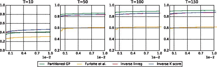
ROC curves for the simulated data with T equal to 10, 50, 100, and 150 time points, for small false positive rates (<0.01). The vertical axis represents the false positive rate and the horizontal axis the true positive rate. ROC, receiver operating characteristics.

4. Discussion

We have introduced a new method for performing GWAS on function-valued traits. Our model is extremely flexible in its capacity to handle a wide range of functional forms. This flexibility is achieved by using a nonparametric statistical model based on RBF GPs. Computations in this model are efficient when time points are aligned and traits are not missing, here scaling only cubically with the number of time points as opposed to cubic in the product of number of time points times individuals, as would be the case in a naive computation. We have also outlined how to do efficient computations even in the presence of missing trait data or unaligned samples. In a comparison against three other models on synthetic data, each with different characteristics and ways of handling the problem, we achieved maximal power, and maximal ability to discriminate null versus alternative tests as judged by an ROC curve. Our model is especially good at handling traits with many time points.

One downside of the model as presented is that the null model is not nested inside the alternative model, making computation of calibrated p values without permutations most likely impossible. We were able to bypass this issue by demonstrating empirically that naive application of a likelihood ratio test controls the type 1 error, yielding extremely conservative p values. However, we are currently investigating a version of the Partitioned GP model that has its null model nested in the alternative model and is, therefore, likely to yield calibrated p values and, therefore, potentially a larger power gain. In this model, the partitions of the alternative model are all placed within a single Gaussian, with correlation parameters for each pair of alleles dictating how similar the GP for each allele should be. When these parameters are equal to 1, we obtain the present alternative model. When these parameters are 0, we obtain the null model, thereby making it nested inside of the alternative. Other directions of interest are to extend this type of modeling approach to testing sets of SNPs rather than only SNPs, and to incorporate model-based warping of the phenotype so as to coerce the data to better adhere to the Gaussian residual assumption (Fusi et al., 2014).

Footnotes

Acknowledgments

We thank Leigh Johnston, Ciprian Crainiceanu, Bobby Kleinberg, and Praneeth Netrapalli for discussion, the anonymous reviewers for helpful feedback, and Carl Kadie for allowing use of his HPC cluster code. Funding for CARe genotyping was provided by NHLBI, contract N01-HC-65226.

Author Disclosure Statement

N.F. and J.L. are employees of Microsoft.

References

Chung

, and Zou

2014. Mixed-effects models for GAW18 longitudinal blood pressure data. BMC Proc. 8, S87.

Das

, Li

, Wang

, et al. 2011. A dynamic model for genome-wide association studies. Hum. Genet., 129, 629–639.

Ding

, Kurowski

B.G.

, He

, et al. 2014. Modeling of multivariate longitudinal phenotypes in family genetic studies with Bayesian multiplicity adjustment. BMC Proc. 8, S69.

Furlotte

N.A.

, Eskin

, and Eyheramendy

2012. Genome-wide association mapping with longitudinal data. Genet. Epidemiol., 36, 463–471.

Fusi

, Lippert

, Lawrence

N.D.

, et al. 2014. Warped linear mixed models for the genetic analysis of transformed phenotypes. Nat. Commun., 5, 4890.

, Zhang

, Lee

, et al. 2015. Set-based tests for genetic association in longitudinal studies. Biometrics, 71, 606–615.

Jaffa

, Gebregziabher

, and Jaffa

A.A.

2015. Analysis of multivariate longitudinal kidney function outcomes using generalized linear mixed models. J. Transl. Med., 13, 192.

Kang

H.M.

, Zaitlen

N.A.

, Wade

C.M.

, et al. 2008. Efficient control of population structure in model organism association mapping. Genetics, 178, 1709–1723.

Kendziorski

C.M.

, Cowley

A.W.

, Greene

A.S.

, et al. 2002. Mapping baroreceptor function to genome: A mathematical modeling approach. Genetics, 160, 1687–1695.

10.

Lippert

, Listgarten

, Liu

, et al. 2011. FaST linear mixed models for genome-wide association studies. Nat. Methods, 8, 833–835.

11.

Listgarten

, Kadie

, Schadt

E.E.

, et al. 2010. Correction for hidden confounders in the genetic analysis of gene expression. Proc. Natl Acad. Sci., 107, 16465–16470.

12.

Listgarten

, Lippert

, Kang

E.Y.

, et al. 2013. A powerful and efficient set test for genetic markers that handles confounders. Bioinformatics, 29, 1526–1533.

13.

Musolf

, Nato

A.Q.

, Londono

, et al. 2014. Mapping genes with longitudinal phenotypes via Bayesian posterior probabilities. BMC Proc. 8, S81.

14.

Price

A.L.

, Patterson

N.J.

, Plenge

R.M.

, et al. 2006. Principal components analysis corrects for stratification in genome-wide association studies. Nat. Genet., 38, 904–909.

15.

Quiñonero Candela

, and Rasmussen

C.E.

2005. A unifying view of sparse approximate gaussian process regression. J. Mach. Learn. Res., 6, 1939–1959.

16.

Rasmussen

C.E.

, and Williams

C.K.I.

2005. Gaussian Processes for Machine Learning (Adaptive Computation and Machine Learning). The MIT Press; Cambridge, MA USA.

17.

Shim

, and Stephens

2015. Wavelet-based genetic association analysis of functional phenotypes arising from high-throughput sequencing assays. Ann. Appl. Stat., 9, 665–686.

18.

Sikorska

, Montazeri

N.M.

, Uitterlinden

, et al. 2015. GWAS with longitudinal phenotypes: Performance of approximate procedures. Eur. J. Hum. Genet., 23, 1384–1391.

19.

Smith

E.N.

, Chen

, Kähönen

, et al. 2010. Longitudinal genome-wide association of cardiovascular disease risk factors in the Bogalusa heart study. PLoS Genet. 6, e1001094.

20.

Stegle

, Denby

K.J.

, Cooke

E.J.

, et al. 2010. A robust Bayesian two-sample test for detecting intervals of differential gene expression in microarray time series. J. Comput. Biol., 17, 355–367.

21.

Stegle

, Lippert

, Mooij

J.M.

, et al. 2011. Efficient inference in matrix-variate gaussian models with \ iid observation noise, 24, 630–638. In Shawe-Taylor

, Zemel

, Bartlett

, et al., eds. Advances in Neural Information Processing Systems. Curran Associates, Inc.

22.

Titsias

M.K.

2009. Variational learning of inducing variables in sparse gaussian processes. Artif. Intell. Stat., 12, 567–574.

23.

Wang

2012. Linear mixed effects model for a longitudinal genome wide association study of lipid measures in type 1 diabetes linear mixed effects model for a longitudinal genome wide association study of lipid measures in type 1 diabetes [Master's thesis]. McMaster University.

24.

M.C.

, Kraft

, Epstein

M.P.

, et al. 2010. Powerful SNP-set analysis for case-control genome-wide association studies. Am. J. Hum. Genet., 86, 929–942.

25.

, Pressoir

, Briggs

W.H.

, et al. 2006. A unified mixed-model method for association mapping that accounts for multiple levels of relatedness. Nat. Genet., 38, 203–208.

26.

Zhang

1997. Multivariate adaptive splines for analysis of longitudinal data. J. Comput. Graph. Stat., 6, 74–91.