Variability in Metagenomic Count Data and Its Influence on the Identification of Differentially Abundant Genes

Abstract

Metagenomics is the study of microorganisms in environmental and clinical samples using high-throughput sequencing of random fragments of their DNA. Since metagenomics does not require any prior culturing of isolates, entire microbial communities can be studied directly in their natural state. In metagenomics, the abundance of genes is quantified by sorting and counting the DNA fragments. The resulting count data are high-dimensional and affected by high levels of technical and biological noise that make the statistical analysis challenging. In this article, we introduce an hierarchical overdispersed Poisson model to explore the variability in metagenomic data. By analyzing three comprehensive data sets, we show that the gene-specific variability varies substantially between genes and is dependent on biological function. We also assess the power of identifying differentially abundant genes and show that incorrect assumptions about the gene-specific variability can lead to unacceptable high rates of false positives. Finally, we evaluate shrinkage approaches to improve the variance estimation and show that the prior choice significantly affects the statistical power. The results presented in this study further elucidate the complex variance structure of metagenomic data and provide suggestions for accurate and reliable identification of differentially abundant genes.

1. Introduction

Metagenomics is the study of microbial communities by direct sequencing of DNA from environmental and clinical samples (Handelsman et al., 1998). The resulting data consist of assorted nucleotide fragments that are randomly selected from the microorganisms present in the analyzed sample. The vast majority (>99%) of all microorganisms are difficult to cultivate using standard protocols; therefore, metagenomics offers a holistic approach to analyze them in their natural state (Hugenholtz et al., 1998; Schloss and Handelsman, 2005). The rapid development of high-throughput DNA sequencing has made metagenomics applicable in many areas. Metagenomics has, for example, been used to investigate changes in the human microbiota and its relation to diseases such as diabetes and Crohn's disease (Turnbaugh et al., 2007; Qin et al., 2010, 2012; Cho and Blaser, 2012; Karlsson et al., 2013). In ecology, metagenomics has been used to characterize the taxonomic diversity and the molecular function of complex microbial communities and ecosystems (Tringe et al., 2005; Edwards et al., 2015). In the environmental sciences, metagenomics has been used to investigate differences between microorganisms living in polluted and pristine regions (Kristiansson et al., 2011; Yanga et al., 2014).

In gene-centric analysis, metagenomes are characterized based on their gene content (Hugenholtz and Tyson, 2008). The abundance of each gene is quantified by sorting and counting the fragments present in the metagenome. In brief, the generated sequence reads are first filtered based on their quality and then aligned to a reference database, typically consisting of a collection of sequenced microbial genomes and/or a gene catalog (Wooley et al., 2010; Li et al., 2014). The genes within the database are annotated based on their biochemical functions, inferred from gene profiles such as clusters of orthologous genes (COGs), TIGRFAMs, and PFAMs (Powell et al., 2011; Haft et al., 2013; Finn et al., 2016), metabolic pathway databases (e.g., KEGG) (Kanehisa et al., 2008), or from more specialized databases targeting more specific functions, such as antibiotic resistance (McArthur et al., 2013; Ma et al., 2014). Finally, the abundance of each annotated function is estimated by counting the number of matching sequence reads, a process that is occasionally referred to as “binning” (Boulund et al., 2015). The end result is a table of counts that describes the number of reads that matched to each functional category in each sample.

Metagenomic data are affected by high levels of variability, which makes analysis difficult (Wooley and Ye, 2009). The abundance of a gene typically varies considerably between samples because of both technical and biological reasons. The technical variation arises, for example, from the DNA extraction, which is known to often be biased toward specific groups of organisms (Morgan et al., 2010). Sample handling can also result in contamination, which in extreme cases has been reported to correspond to as much as 60% of the sequenced reads (Schmieder and Edwards, 2011). Next-generation DNA sequencing also has a high error rate, which can reach 1% of base calls (Quail et al., 2012). The reference database used in the binning process is often extremely sparse, reflecting only a minority of the organisms present in the studied microbial community. There are, for example, currently less than 4000 fully completed bacterial genomes (Land et al., 2015). However, the prokaryotic diversity is vast, with at least 10 million estimated bacterial species (Curtis et al., 2002; Pedrós-Alió, 2006). Hence, most DNA fragments generated in metagenomics have never been seen before by man, which makes the binning process inexact, and nonrepresented genes may be misclassified or missed completely (Wooley et al., 2010; Rinke et al., 2013).

Furthermore, microbial communities are inherently complex with considerable biological variation both spatially between sites and individuals but also over time (Caporaso et al., 2011). This variation is often driven by factors specific to the environments studied, for example, pH, salinity, and moisture in soil (Fierer et al., 2012) and age, diet, and host genetics in the human gut (Lozupone et al., 2012). Thus, although the technical and biological variability between metagenomes is often substantial, it has not yet been studied in detail.

The aim of most gene-centric metagenomic experiments is to identify differences in the gene frequencies between two or more conditions (Tringe et al., 2005). Several statistical methods have been suggested for identifying differentially abundant genes in metagenomic gene count data. These methods include standard statistical methods, such as tests for count data, for example, Fisher's exact test (Parks and Beiko, 2010) and Poisson generalized linear models (GLMs) (Kristiansson et al., 2009), as well as procedures based on normal approximations (e.g., variance stabilizing transformations in combination with t-tests) (Sanli et al., 2013) and nonparametric methods (Wilcoxon–Mann Whitney U test) (Segata et al., 2011). More advanced models, which aim to specifically describe the variation exhibited in metagenomic data, have also been proposed (e.g., metagenomeSeq and RAIDA) (Paulson et al., 2013; Sohn et al., 2015). The methods suggested to date apply fundamentally different assumptions about the variability exhibited in metagenomic data. For example, metagenomeSeq and t-tests assume a gene-specific between-sample variability. This is in contrast to Fisher's exact test and the Poisson GLM, which assume no between-sample variability. However, the validity of these assumptions and their impact on the performance of identifying differentially abundant genes have not yet been investigated thoroughly.

The number of samples in a typical metagenomic study is typically small (often <10), thus making it difficult to accurately estimate the gene-specific variability (Knight et al., 2012). Shrinkage-based estimation, which moderates variance estimates by combining information from the underlying data with the variance estimates from other genes, has been shown to increase the performance of statistical inference in high-dimensional molecular data (Smyth, 2004; Sjögren et al., 2007). Such methods have also recently been successfully applied within the field of RNA sequencing (Nookaew et al., 2012; Soneson and Delorenzi, 2013). However, shrinkage methods developed for RNA-seq data have been shown to have mixed performance on metagenomic data (Jonsson et al., 2016), which is likely to be caused by suboptimal distributional assumptions. Whereas RNA-seq data are structurally similar to metagenomic data, the underlying variability is considerably different. The variability in RNA-seq data arises from differences in expression patterns between a single type of cells. In metagenomics, however, the variability arises, to a large extent, from the sampling of entire microbial ecosystems. Thus, the impact of the distribution assumptions for shrinkage-based methods needs to be further evaluated for metagenomic gene count data.

The aim of this article is to analyze the variance structure of gene abundances in metagenomes. First, we introduce a hierarchical overdispersed Poisson model to describe metagenomic gene count data. The model is used to estimate the gene-specific variability in three comprehensive metagenomes, representing both different environments and sequencing technologies. Our results show that genes differ considerably in their variability and that these differences are associated with biological functions and conserved between metagenomes. Next, we use resampling of the three metagenomes to assess the statistical power of detecting differentially abundant genes under the model. We show that incorrect variance assumptions lead to unacceptably high rates of false positives. Finally, we quantify the effect of shrinkage-based variance estimation on the analysis of metagenomic data and show that the performance is dependent on the distribution assumptions. Taken together, our results highlight the importance of sound modeling for reliable interpretation of metagenomic gene count data.

2. Results

This study was based on the analysis of three comprehensive metagenomic data sets representing different environment types and sequencing techniques (Table 1). The first two data sets were from human gut metagenomes, in which the first one consisted of 74 individuals (Human gut I) sequenced using Illumina technology (Qin et al., 2012) and the second one (Human gut II) consisted of 110 individuals sequenced using massively parallel pyrosequencing (Yatsunenko et al., 2012). The third data set (Marine) consisted of 44 metagenomes sampled from ocean surface water and sequenced using Illumina technology (Sunagawa et al., 2015). All three data sets were functionally annotated and quantified based on COGs (Section 4) (Huerta-Cepas et al., 2015). The number of detected COGs ranged from 2354 to 4372 for the three data sets. For ease of reading, the COGs will be referred to as genes throughout the article.

Table 1.

Description of the Three Included Data Sets

	Human gut I	Human gut II	Marine
Reference	Qin 2012	Yatsunenko 2012	Sunagawa 2015
Sequencing platform	Illumina	454-pyrosequencing	Illumina
Number of samples	74	110	45
Average reads per sample	32,315,932	155,890	324,004,492
Number of genes	3573	2354	4372
Sampling point	Fecal samples	Fecal samples	Oceanic surface water

The number of genes refers to the number of COGs remaining in the full data sets after filtering.

The gene count data were modeled as follows. The abundance of each gene was assumed to follow a log-normal distribution with gene-specific mean and variance parameters. Conditioned on the gene abundance, the random sampling of DNA fragments was assumed to follow a Poisson distribution. The observed gene counts will then be distributed according to a Poisson-log-normal distribution, which is, compared to the original Poisson distribution, overdispersed with a quadratic relationship between its mean and variance (Aitchison and Ho, 1989), that is, \documentclass{aastex}\usepackage{amsbsy}\usepackage{amsfonts}\usepackage{amssymb}\usepackage{bm}\usepackage{mathrsfs}\usepackage{pifont}\usepackage{stmaryrd}\usepackage{textcomp}\usepackage{portland, xspace}\usepackage{amsmath, amsxtra}\pagestyle{empty}\DeclareMathSizes{10}{9}{7}{6}\begin{document} \begin{align*} Var [ {Y_{ij}} ] = { \mu _i} + { \phi _i} \mu _i^2 , \end{align*} \end{document}

where \documentclass{aastex}\usepackage{amsbsy}\usepackage{amsfonts}\usepackage{amssymb}\usepackage{bm}\usepackage{mathrsfs}\usepackage{pifont}\usepackage{stmaryrd}\usepackage{textcomp}\usepackage{portland, xspace}\usepackage{amsmath, amsxtra}\pagestyle{empty}\DeclareMathSizes{10}{9}{7}{6}\begin{document} $${Y_{ij}}$$ \end{document} denotes the counts of gene i in sample j, \documentclass{aastex}\usepackage{amsbsy}\usepackage{amsfonts}\usepackage{amssymb}\usepackage{bm}\usepackage{mathrsfs}\usepackage{pifont}\usepackage{stmaryrd}\usepackage{textcomp}\usepackage{portland, xspace}\usepackage{amsmath, amsxtra}\pagestyle{empty}\DeclareMathSizes{10}{9}{7}{6}\begin{document} $${ \mu _i}$$ \end{document} is the abundance of gene i, and \documentclass{aastex}\usepackage{amsbsy}\usepackage{amsfonts}\usepackage{amssymb}\usepackage{bm}\usepackage{mathrsfs}\usepackage{pifont}\usepackage{stmaryrd}\usepackage{textcomp}\usepackage{portland, xspace}\usepackage{amsmath, amsxtra}\pagestyle{empty}\DeclareMathSizes{10}{9}{7}{6}\begin{document} $${ \phi _i}$$ \end{document} is the gene-specific overdispersion. Note that if the overdispersion is zero, that is, \documentclass{aastex}\usepackage{amsbsy}\usepackage{amsfonts}\usepackage{amssymb}\usepackage{bm}\usepackage{mathrsfs}\usepackage{pifont}\usepackage{stmaryrd}\usepackage{textcomp}\usepackage{portland, xspace}\usepackage{amsmath, amsxtra}\pagestyle{empty}\DeclareMathSizes{10}{9}{7}{6}\begin{document} $${ \phi _i} = 0$$ \end{document} , then the counts for gene i will follow a standard Poisson distribution and thus have its variance equal to its mean. The model fits within the flexible framework of a generalized linear mixed model. See Section 4 for the full details of the model and the Markov chain Monte Carlo-based parameter estimation.

2.1. Overdispersion differs between genes but shows consistency across data sets

From a statistical standpoint, the variability of a gene will affect the power to detect an effect. To assess the variability in metagenomic data, the model (without effect parameter) was fit to each of the three metagenomic data sets and the posterior mean of the gene-specific overdispersion was calculated. Although the data originated from different environments and sequencing techniques, the gene-specific overdispersion \documentclass{aastex}\usepackage{amsbsy}\usepackage{amsfonts}\usepackage{amssymb}\usepackage{bm}\usepackage{mathrsfs}\usepackage{pifont}\usepackage{stmaryrd}\usepackage{textcomp}\usepackage{portland, xspace}\usepackage{amsmath, amsxtra}\pagestyle{empty}\DeclareMathSizes{10}{9}{7}{6}\begin{document} $${ \phi _i}$$ \end{document} in all three data sets exhibited similar distributions (Fig. 1). The median overdispersion was the highest in the Human gut I data set (0.73), followed by the Human gut II (0.60) and Marine data sets (0.58). Furthermore, the Human gut I and Marine data sets showed heavier tails toward higher values, suggesting that they contain a larger proportion of highly variable genes (upper deciles were 33 and 28 for Human gut I and Marine, respectively, compared with 4.8 for Human gut II). Interestingly, the Marine data contained more low variability genes (lower decile of 0.012 for Marine compared with 0.039 and 0.035 for the Human gut I and II data sets), suggesting a larger proportion of stable genes. There was a marked trend of genes with similar overdispersion in all three data sets (Fig. 2). This trend was especially clear for genes with low overdispersion, whereas genes with a higher overdispersion were more diverse. The Spearman correlation of the gene-specific overdispersion was the highest between Human gut I and Human gut II (0.62) but only slightly lower between Human gut I and Marine (0.56) and between Human gut II and Marine (0.50).

FIG. 1.

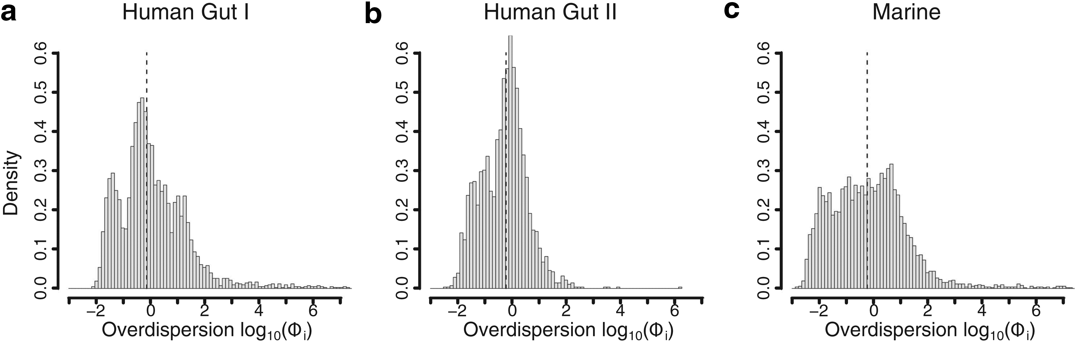
Histograms over the posterior mean ( \documentclass{aastex}\usepackage{amsbsy}\usepackage{amsfonts}\usepackage{amssymb}\usepackage{bm}\usepackage{mathrsfs}\usepackage{pifont}\usepackage{stmaryrd}\usepackage{textcomp}\usepackage{portland, xspace}\usepackage{amsmath, amsxtra}\pagestyle{empty}\DeclareMathSizes{10}{9}{7}{6}\begin{document} $${ \rm{lo}}{{ \rm{g}}_{10}}$$ \end{document} transformed) of the overdispersion parameter, \documentclass{aastex}\usepackage{amsbsy}\usepackage{amsfonts}\usepackage{amssymb}\usepackage{bm}\usepackage{mathrsfs}\usepackage{pifont}\usepackage{stmaryrd}\usepackage{textcomp}\usepackage{portland, xspace}\usepackage{amsmath, amsxtra}\pagestyle{empty}\DeclareMathSizes{10}{9}{7}{6}\begin{document} $${ \phi _i}$$ \end{document} , for every gene in the three data sets: Human gut I (a), Human gut II (b) and Marine (c). The dashed line indicates the median overdispersion.

FIG. 2.

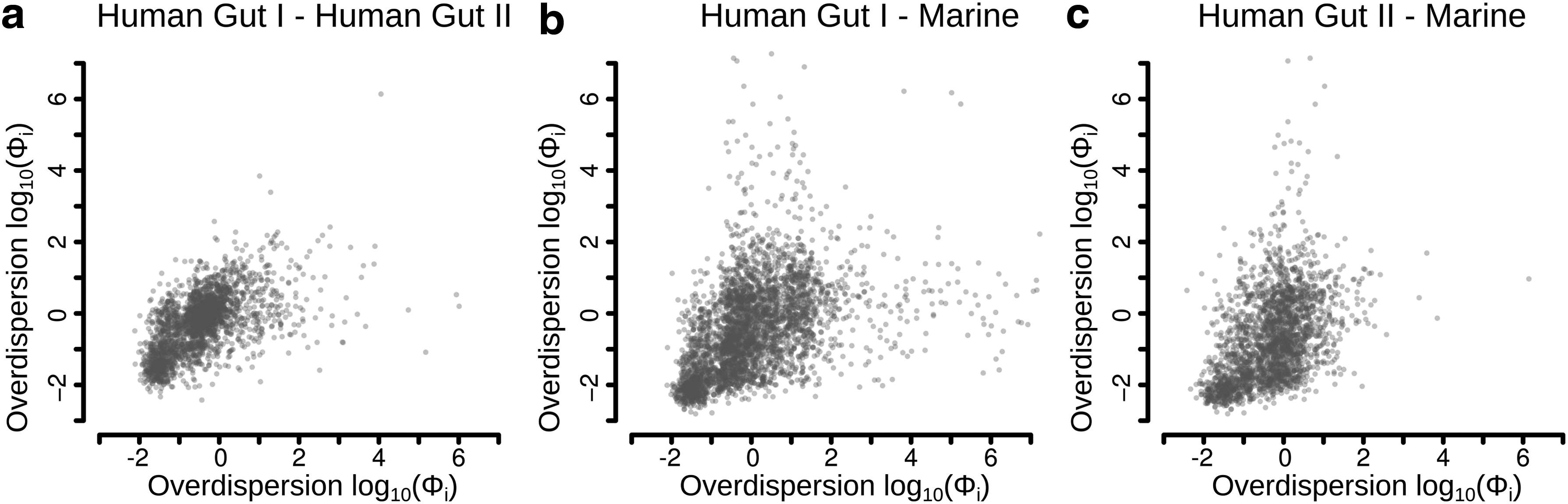
Pairwise scatterplots of the posterior mean of the overdispersion, \documentclass{aastex}\usepackage{amsbsy}\usepackage{amsfonts}\usepackage{amssymb}\usepackage{bm}\usepackage{mathrsfs}\usepackage{pifont}\usepackage{stmaryrd}\usepackage{textcomp}\usepackage{portland, xspace}\usepackage{amsmath, amsxtra}\pagestyle{empty}\DeclareMathSizes{10}{9}{7}{6}\begin{document} $${ \phi _i}$$ \end{document} . ( \documentclass{aastex}\usepackage{amsbsy}\usepackage{amsfonts}\usepackage{amssymb}\usepackage{bm}\usepackage{mathrsfs}\usepackage{pifont}\usepackage{stmaryrd}\usepackage{textcomp}\usepackage{portland, xspace}\usepackage{amsmath, amsxtra}\pagestyle{empty}\DeclareMathSizes{10}{9}{7}{6}\begin{document} $${ \rm{lo}}{{ \rm{g}}_{10}}$$ \end{document} transformed) for genes present in each pair of data sets. Between Human gut I and Human gut II, 2309 genes overlapped (a); between Human gut I and Marine, 3369 genes overlapped (b); and between Human gut II and Marine, 2275 genes overlapped (c).

To investigate whether the gene-specific overdispersion is associated with biological functions, we mapped each COG to Gene Ontology (GO) terms (Gene Ontology Consortium, 2015). Each GO term was then tested for enrichment of genes with low and high overdispersion (see Section 4). For the 25% of genes with the lowest overdispersion, there was a high number of significant GO terms (p < 0.001) for all three data sets (246, 69, and 276 for Human gut I, Human gut II, and Marine, respectively) (Supplementary Table S1). A large proportion of these terms overlapped between data sets, with as many as 60 significant GO terms identified for all three data sets. These GO terms were associated with fundamental biological functions, such as metabolism of amino acids and nucleotides, translation, and various biosynthetic processes. Furthermore, the gene-specific overdispersion was also found to be substantially lower for single copy genes. Thirty-five genes used in a study on effective genome size had an average overdispersion of less than 0.04 across the three data sets (Raes et al., 2007).

The enrichment test for genes with high overdispersion yielded considerably fewer significant GO terms (4, 0, and 48 for Human gut I, Human gut II, and Marine, respectively) (Supplementary Table S2) with no overlap between any of the data sets. Although the signal was weaker, both GO terms associated with horizontal gene transfer and formation of the cell wall were highly ranked in both Human gut I and Human gut II. This result indicates that functions for adapting to the local environment have higher overdispersion. This was different from the 48 significant GO terms found in the Marine data set, of which a majority were related to eukaryotic biological functions, suggesting a large variation in bacterial–eukaryal species composition. Thus, these results suggest that genes with a low overdispersion show similarities between metagenomes whereas genes with a high overdispersion are less defined.

2.2. Modeling of the gene-specific overdispersion improves gene ranking

An important step in metagenomic studies is to rank genes based on their differential abundance between conditions. The accuracy of the gene ranking is dependent on the estimation of the gene-specific variance. We, therefore, investigated the performance under three different model assumptions that closely resemble previously suggested methods for the analysis of count data but that use fundamentally different assumptions regarding the gene-specific overdispersion (Robinson and Smyth, 2008; Kristiansson et al., 2009). The first model (Model 1) assumes that there is no overdispersion (i.e., \documentclass{aastex}\usepackage{amsbsy}\usepackage{amsfonts}\usepackage{amssymb}\usepackage{bm}\usepackage{mathrsfs}\usepackage{pifont}\usepackage{stmaryrd}\usepackage{textcomp}\usepackage{portland, xspace}\usepackage{amsmath, amsxtra}\pagestyle{empty}\DeclareMathSizes{10}{9}{7}{6}\begin{document} $${ \phi _i} = 0$$ \end{document} for all genes) and thus uses a standard Poisson distribution to model the count data. Model 2 assumes that all genes have the same overdispersion (i.e., \documentclass{aastex}\usepackage{amsbsy}\usepackage{amsfonts}\usepackage{amssymb}\usepackage{bm}\usepackage{mathrsfs}\usepackage{pifont}\usepackage{stmaryrd}\usepackage{textcomp}\usepackage{portland, xspace}\usepackage{amsmath, amsxtra}\pagestyle{empty}\DeclareMathSizes{10}{9}{7}{6}\begin{document} $${ \phi _i}$$ \end{document} is the same for all genes i). Finally, Model 3 assumes a gene-specific overdispersion, where \documentclass{aastex}\usepackage{amsbsy}\usepackage{amsfonts}\usepackage{amssymb}\usepackage{bm}\usepackage{mathrsfs}\usepackage{pifont}\usepackage{stmaryrd}\usepackage{textcomp}\usepackage{portland, xspace}\usepackage{amsmath, amsxtra}\pagestyle{empty}\DeclareMathSizes{10}{9}{7}{6}\begin{document} $${ \phi _i}$$ \end{document} is estimated for each gene individually. See Section 4 for full details about the three models. The impact of the model assumptions on the ability to rank genes was evaluated on artificial metagenomic data generated by resampling. For each of the three data sets in this study, 10 + 10 samples were repeatedly sampled, and effects were added for randomly selected genes using downsampling (see Section 4). This setting retains much of the data structure, particularly the within-sample correlations, that is present in real data.

The ranking performance was summarized using receiver operating characteristic (ROC) curves and the corresponding area under the curve up to a false positive rate (FPR) of 0.1 ( \documentclass{aastex}\usepackage{amsbsy}\usepackage{amsfonts}\usepackage{amssymb}\usepackage{bm}\usepackage{mathrsfs}\usepackage{pifont}\usepackage{stmaryrd}\usepackage{textcomp}\usepackage{portland, xspace}\usepackage{amsmath, amsxtra}\pagestyle{empty}\DeclareMathSizes{10}{9}{7}{6}\begin{document} $$AU{C_{0.1}}$$ \end{document} ) (Fig. 3 and Table 2). Model 3, which allowed for gene-specific overdispersion, had a high and consistent performance across all three data sets with an \documentclass{aastex}\usepackage{amsbsy}\usepackage{amsfonts}\usepackage{amssymb}\usepackage{bm}\usepackage{mathrsfs}\usepackage{pifont}\usepackage{stmaryrd}\usepackage{textcomp}\usepackage{portland, xspace}\usepackage{amsmath, amsxtra}\pagestyle{empty}\DeclareMathSizes{10}{9}{7}{6}\begin{document} $$AU{C_{0.1}}$$ \end{document} of 0.70, 0.73, and 0.75 for Human gut I, Human gut II, and Marine, respectively. The performance was lower for Model 2, which assumed the same overdispersion for all genes, in two data sets ( \documentclass{aastex}\usepackage{amsbsy}\usepackage{amsfonts}\usepackage{amssymb}\usepackage{bm}\usepackage{mathrsfs}\usepackage{pifont}\usepackage{stmaryrd}\usepackage{textcomp}\usepackage{portland, xspace}\usepackage{amsmath, amsxtra}\pagestyle{empty}\DeclareMathSizes{10}{9}{7}{6}\begin{document} $$AU{C_{0.1}}$$ \end{document} 0.56 in Human gut I and 0.63 in Marine), but performed better in Human gut II with an \documentclass{aastex}\usepackage{amsbsy}\usepackage{amsfonts}\usepackage{amssymb}\usepackage{bm}\usepackage{mathrsfs}\usepackage{pifont}\usepackage{stmaryrd}\usepackage{textcomp}\usepackage{portland, xspace}\usepackage{amsmath, amsxtra}\pagestyle{empty}\DeclareMathSizes{10}{9}{7}{6}\begin{document} $$AU{C_{0.1}}$$ \end{document} of 0.73. This is likely a result of the considerably lower average gene count in this data set, which is a result of the different sequencing technique used (massively parallel pyrosequencing instead of Illumina sequencing).

FIG. 3.

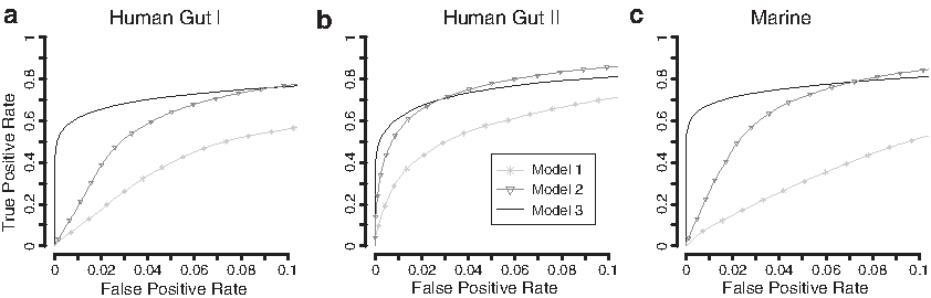
ROC curves for Models 1–3. Model 1 assumes that no overdispersion is present. Model 2 assumes that all genes have the same overdispersion and Model 2 permits gene-specific overdispersion. The ROC curves represent the average curve after 50 repetitions for each of the three data sets, Human Gut I (a), Human Gut II (b), and Marine (c). Group size was set to 10 + 10, and effects were added with a fold change of 3. ROC, receiver operating characteristic.

Table 2.

Area Under the Curve, \documentclass{aastex}\usepackage{amsbsy}\usepackage{amsfonts}\usepackage{amssymb}\usepackage{bm}\usepackage{mathrsfs}\usepackage{pifont}\usepackage{stmaryrd}\usepackage{textcomp}\usepackage{portland, xspace}\usepackage{amsmath, amsxtra}\pagestyle{empty}\DeclareMathSizes{10}{9}{7}{6}\begin{document} $$AU{C_{0.1}}$$ \end{document} , Measurements for Models 1–3 Corresponding to the Receiver Operating Characteristic Curves Presented in Figure 3

	Human gut I	Human gut II	Marine
Model 1	0.356	0.540	0.295
Model 2	0.560	0.733	0.631
Model 3	0.699	0.729	0.751

The group size was set to 10 + 10, and the effect size was set to 3. \documentclass{aastex}\usepackage{amsbsy}\usepackage{amsfonts}\usepackage{amssymb}\usepackage{bm}\usepackage{mathrsfs}\usepackage{pifont}\usepackage{stmaryrd}\usepackage{textcomp}\usepackage{portland, xspace}\usepackage{amsmath, amsxtra}\pagestyle{empty}\DeclareMathSizes{10}{9}{7}{6}\begin{document} $$AU{C_{0.1}}$$ \end{document} indicates that the AUC is measured up to a false positive rate of 0.1.

Finally, Model 3, which assumes no overdispersion, had a very low performance across all three data sets with an \documentclass{aastex}\usepackage{amsbsy}\usepackage{amsfonts}\usepackage{amssymb}\usepackage{bm}\usepackage{mathrsfs}\usepackage{pifont}\usepackage{stmaryrd}\usepackage{textcomp}\usepackage{portland, xspace}\usepackage{amsmath, amsxtra}\pagestyle{empty}\DeclareMathSizes{10}{9}{7}{6}\begin{document} $$AU{C_{0.1}}$$ \end{document} of 0.36, 0.54, and 0.30 for Human gut I, Human gut II, and Marine, respectively. To investigate the FPRs under the different model assumptions, we calculate the proportion of false positives at the top 10% of the ranking lists. (Fig. 4). Model 1 suffered from a large FPR for all data sets with a median proportion of false positives of 0.53, 0.42, and 0.61 for Human gut I, Human gut II, and Marine data sets, respectively. Model 2 had a better performance in which the corresponding median of proportion of false positives was 0.33, 0.25, and 0.28. Model 3 had the best performance on all but the Human gut II data set, medians 0.30, 0.29, and 0.25, and had the most stable performance of all three methods. Thus, incorporation of the gene-specific overdispersion is vital for accurately ranking differentially abundant genes and may, if ignored, result in substantially reduced performance and an excess number of false positives.

FIG. 4.

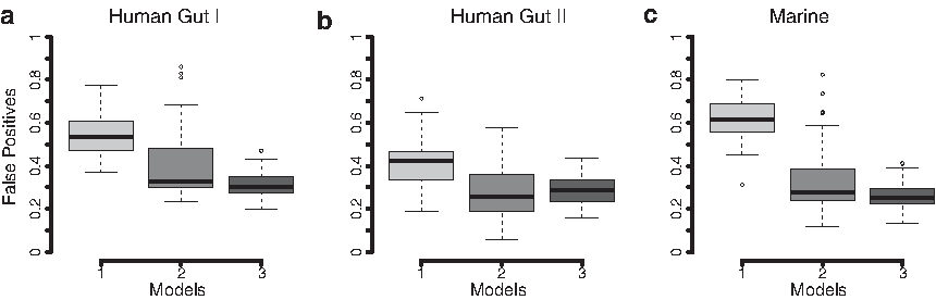
Box plots detailing the proportion of false positives among the top 10% of ranked genes for each of the three different models (Models 1–3). The results are based on 50 runs of resampled data from each data set, Human gut I (a), Human gut II (b), and Marine (c). Group size was set to 10 + 10 and effects were added with a fold change of 3.

2.3. Ranking performance differs between shrinkage priors

Estimating the gene-specific overdispersion is challenging when few samples are available. Shrinkage-based methods, which assume that the gene-specific overdispersion follows a shared prior distribution, are therefore used to increase the robustness. Such methods are established in the analysis of count data for large-scale transcriptomics (using RNA-seq) (Robinson et al., 2010; Love et al., 2014) but have thus far not been thoroughly evaluated for metagenomic data. We, therefore, assessed the performance of the model under different shared prior assumptions. Note that under the Poisson log-normal model used in this study, the gene-specific overdispersion is governed by the parameter \documentclass{aastex}\usepackage{amsbsy}\usepackage{amsfonts}\usepackage{amssymb}\usepackage{bm}\usepackage{mathrsfs}\usepackage{pifont}\usepackage{stmaryrd}\usepackage{textcomp}\usepackage{portland, xspace}\usepackage{amsmath, amsxtra}\pagestyle{empty}\DeclareMathSizes{10}{9}{7}{6}\begin{document} $$\sigma _i^2$$ \end{document} , where \documentclass{aastex}\usepackage{amsbsy}\usepackage{amsfonts}\usepackage{amssymb}\usepackage{bm}\usepackage{mathrsfs}\usepackage{pifont}\usepackage{stmaryrd}\usepackage{textcomp}\usepackage{portland, xspace}\usepackage{amsmath, amsxtra}\pagestyle{empty}\DeclareMathSizes{10}{9}{7}{6}\begin{document} $${ \phi _i} = {e^{ \sigma _i^2}} - 1$$ \end{document} . Three shared priors for \documentclass{aastex}\usepackage{amsbsy}\usepackage{amsfonts}\usepackage{amssymb}\usepackage{bm}\usepackage{mathrsfs}\usepackage{pifont}\usepackage{stmaryrd}\usepackage{textcomp}\usepackage{portland, xspace}\usepackage{amsmath, amsxtra}\pagestyle{empty}\DeclareMathSizes{10}{9}{7}{6}\begin{document} $$\sigma _i^2$$ \end{document} were evaluated, namely, (i) a gamma distribution, (ii) an inverse-gamma distribution, and (iii) a log-normal distribution.

The three shared prior assumptions were compared with the estimates of \documentclass{aastex}\usepackage{amsbsy}\usepackage{amsfonts}\usepackage{amssymb}\usepackage{bm}\usepackage{mathrsfs}\usepackage{pifont}\usepackage{stmaryrd}\usepackage{textcomp}\usepackage{portland, xspace}\usepackage{amsmath, amsxtra}\pagestyle{empty}\DeclareMathSizes{10}{9}{7}{6}\begin{document} $$\sigma _i^2$$ \end{document} using the full data sets (Supplementary Fig. S1). None of the priors provided a perfect fit for any of the data sets. The gamma distribution showed a satisfactory fit for high-variable genes, whereas its tail was too thick for low-variable genes. Conversely, the inverse-gamma distribution showed a good fit for low-variable genes but had a tail that was too thick for high-variable genes. The log-normal distribution had small but consistent deviations for both low- and high-variable genes. The ranking performances of the different prior assumptions were evaluated by artificial data sets using a small group size of 3 + 3 (Section 4) (Fig. 5 and Table 3). The model without shrinkage had, unsurprisingly, the lowest performance for all three data sets with an \documentclass{aastex}\usepackage{amsbsy}\usepackage{amsfonts}\usepackage{amssymb}\usepackage{bm}\usepackage{mathrsfs}\usepackage{pifont}\usepackage{stmaryrd}\usepackage{textcomp}\usepackage{portland, xspace}\usepackage{amsmath, amsxtra}\pagestyle{empty}\DeclareMathSizes{10}{9}{7}{6}\begin{document} $$AU{C_{0.1}}$$ \end{document} of 0.44 (Human gut I), 0.39 (Human gut II), and 0.54 (Marine). The difference between the models with and without shrinkage was particularly large for Human gut II, which is the data set with the lowest sequencing depth. Among the three shared priors, the inverse-gamma prior had the best performance with an \documentclass{aastex}\usepackage{amsbsy}\usepackage{amsfonts}\usepackage{amssymb}\usepackage{bm}\usepackage{mathrsfs}\usepackage{pifont}\usepackage{stmaryrd}\usepackage{textcomp}\usepackage{portland, xspace}\usepackage{amsmath, amsxtra}\pagestyle{empty}\DeclareMathSizes{10}{9}{7}{6}\begin{document} $$AU{C_{0.1}}$$ \end{document} of 0.48, 0.45, and 0.58 for the three data sets, respectively. The performance of the log-normal prior was almost as high (0.48, 0.45, and 0.57 for Human gut I, Human gut II, and Marine, respectively), whereas the performance of the gamma prior was the worst with \documentclass{aastex}\usepackage{amsbsy}\usepackage{amsfonts}\usepackage{amssymb}\usepackage{bm}\usepackage{mathrsfs}\usepackage{pifont}\usepackage{stmaryrd}\usepackage{textcomp}\usepackage{portland, xspace}\usepackage{amsmath, amsxtra}\pagestyle{empty}\DeclareMathSizes{10}{9}{7}{6}\begin{document} $$AU{C_{0.1}}$$ \end{document} of 0.46, 0.44, and 0.56 for the three data sets, respectively.

FIG. 5.

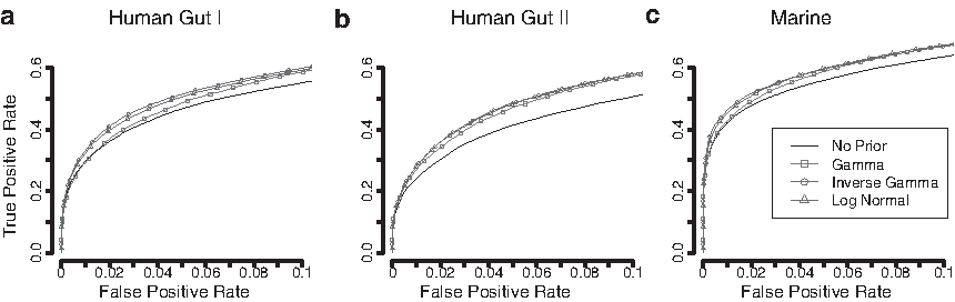
ROC curves for comparing the ranking performance of the shrinkage priors using all genes in each data set. The group size was set to 3 + 3 and effects were added with a fold change of 3. The ROC curves represent the average curve generated from 50 resampled data sets from Human Gut I (a), Human Gut II (b), and Marine (c).

Table 3.

Area Under the Curve, \documentclass{aastex}\usepackage{amsbsy}\usepackage{amsfonts}\usepackage{amssymb}\usepackage{bm}\usepackage{mathrsfs}\usepackage{pifont}\usepackage{stmaryrd}\usepackage{textcomp}\usepackage{portland, xspace}\usepackage{amsmath, amsxtra}\pagestyle{empty}\DeclareMathSizes{10}{9}{7}{6}\begin{document} $$AU{C_{0.1}}$$ \end{document} , Measurements for the Shrinkage Priors Evaluated in All the Genes in Each Data Set Corresponding to the Receiver Operating Characteristic Curves Presented in Figure 5

	Human gut I	Human gut II	Marine
No prior	0.440	0.388	0.539
Gamma	0.457	0.440	0.563
Inverse gamma	0.484	0.452	0.576
Log-normal	0.476	0.450	0.575

The group size was set to 3 + 3, and the effect size was set to 3. \documentclass{aastex}\usepackage{amsbsy}\usepackage{amsfonts}\usepackage{amssymb}\usepackage{bm}\usepackage{mathrsfs}\usepackage{pifont}\usepackage{stmaryrd}\usepackage{textcomp}\usepackage{portland, xspace}\usepackage{amsmath, amsxtra}\pagestyle{empty}\DeclareMathSizes{10}{9}{7}{6}\begin{document} $$AU{C_{0.1}}$$ \end{document} indicates that the AUC is measured up to a false positive rate of 0.1.

To further assess how the choice of the shared priors impacts genes with high and low variability, the data were stratified based on their overdispersion estimated from the full data sets (i.e., Fig. 1). For the genes with a low overdispersion, the differences between the shared priors were more pronounced. The inverse-gamma prior still had the best performance with \documentclass{aastex}\usepackage{amsbsy}\usepackage{amsfonts}\usepackage{amssymb}\usepackage{bm}\usepackage{mathrsfs}\usepackage{pifont}\usepackage{stmaryrd}\usepackage{textcomp}\usepackage{portland, xspace}\usepackage{amsmath, amsxtra}\pagestyle{empty}\DeclareMathSizes{10}{9}{7}{6}\begin{document} $$AU{C_{0.1}}$$ \end{document} of 0.81, 0.73, and 0.91, whereas the gamma prior had the worst performance with \documentclass{aastex}\usepackage{amsbsy}\usepackage{amsfonts}\usepackage{amssymb}\usepackage{bm}\usepackage{mathrsfs}\usepackage{pifont}\usepackage{stmaryrd}\usepackage{textcomp}\usepackage{portland, xspace}\usepackage{amsmath, amsxtra}\pagestyle{empty}\DeclareMathSizes{10}{9}{7}{6}\begin{document} $$AU{C_{0.1}}$$ \end{document} of 0.77, 0.69, and 0.88 (Fig. 6 and Table 4). However, for the genes with high overdispersion, the relative order in performance was reversed (Fig 7 and Table 5). Here, the gamma prior resulted in the highest performance with \documentclass{aastex}\usepackage{amsbsy}\usepackage{amsfonts}\usepackage{amssymb}\usepackage{bm}\usepackage{mathrsfs}\usepackage{pifont}\usepackage{stmaryrd}\usepackage{textcomp}\usepackage{portland, xspace}\usepackage{amsmath, amsxtra}\pagestyle{empty}\DeclareMathSizes{10}{9}{7}{6}\begin{document} $$AU{C_{0.1}}$$ \end{document} of 0.47, 0.49, and 0.53, whereas the inverse gamma had the lowest performance of the priors with \documentclass{aastex}\usepackage{amsbsy}\usepackage{amsfonts}\usepackage{amssymb}\usepackage{bm}\usepackage{mathrsfs}\usepackage{pifont}\usepackage{stmaryrd}\usepackage{textcomp}\usepackage{portland, xspace}\usepackage{amsmath, amsxtra}\pagestyle{empty}\DeclareMathSizes{10}{9}{7}{6}\begin{document} $$AU{C_{0.1}}$$ \end{document} of 0.43, 0.46, and 0.48. Notably, on the Marine data set, the model with the inverse-gamma prior performed almost as poorly as the model without any shrinkage (Fig. 6c).

FIG. 6.

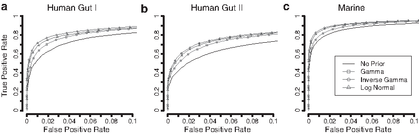
ROC curves for comparing the ranking performance of the shrinkage priors using only the genes with low overdispersion in each data set. The split in overdispersion was based on the estimates from the full data set. The group size was set to 3 + 3 and effects were added with a fold change of 3. The ROC curves represent the average curve generated from 50 resampled data sets from Human Gut I (a), Human Gut II (b), and Marine (c).

FIG. 7.

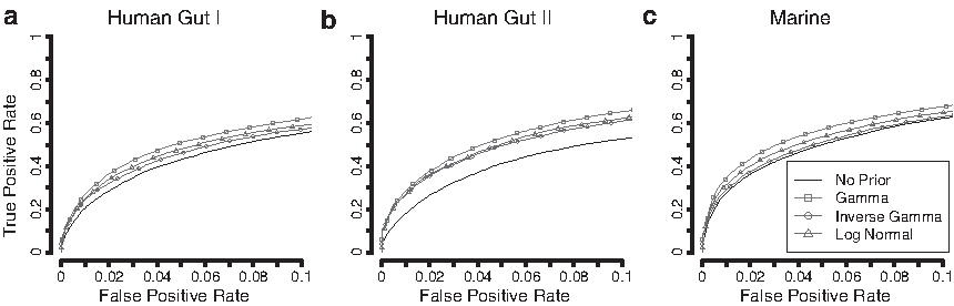
ROC curves for comparing the ranking performance of the shrinkage priors using only the genes with high overdispersion in each data set. The split in overdispersion was based on the estimates from the full data set. The group size was set to 3 + 3 and effects were added with a fold change of 10. The ROC curves represent the average curve generated from 50 resampled data sets from Human Gut I (a), Human Gut II (b), and Marine (c).

Table 4.

Area Under the Curve, \documentclass{aastex}\usepackage{amsbsy}\usepackage{amsfonts}\usepackage{amssymb}\usepackage{bm}\usepackage{mathrsfs}\usepackage{pifont}\usepackage{stmaryrd}\usepackage{textcomp}\usepackage{portland, xspace}\usepackage{amsmath, amsxtra}\pagestyle{empty}\DeclareMathSizes{10}{9}{7}{6}\begin{document} $$AU{C_{0.1}}$$ \end{document} , Measurements for the Shrinkage Priors When Evaluated on Only the Genes with Low Overdispersion Corresponding to the Receiver Operating Characteristic Curves Presented in Figure 6

	Human gut I	Human gut II	Marine
No prior	0.707	0.603	0.856
Gamma	0.768	0.688	0.883
Inverse gamma	0.815	0.728	0.913
Log-normal	0.795	0.714	0.905

Table 5.

Area Under the Curve, \documentclass{aastex}\usepackage{amsbsy}\usepackage{amsfonts}\usepackage{amssymb}\usepackage{bm}\usepackage{mathrsfs}\usepackage{pifont}\usepackage{stmaryrd}\usepackage{textcomp}\usepackage{portland, xspace}\usepackage{amsmath, amsxtra}\pagestyle{empty}\DeclareMathSizes{10}{9}{7}{6}\begin{document} $$AU{C_{0.1}}$$ \end{document} , Measurements for the Shrinkage Priors on Only the Genes with High Overdispersion Corresponding to the Receiver Operating Characteristic Curves Presented in Figure 7

	Human gut I	Human gut II	Marine
No prior	0.399	0.378	0.468
Gamma	0.469	0.494	0.533
Inverse gamma	0.428	0.461	0.479
Log-normal	0.444	0.470	0.503

The group size was set to 3 + 3, and the effect size was set to 7. \documentclass{aastex}\usepackage{amsbsy}\usepackage{amsfonts}\usepackage{amssymb}\usepackage{bm}\usepackage{mathrsfs}\usepackage{pifont}\usepackage{stmaryrd}\usepackage{textcomp}\usepackage{portland, xspace}\usepackage{amsmath, amsxtra}\pagestyle{empty}\DeclareMathSizes{10}{9}{7}{6}\begin{document} $$AU{C_{0.1}}$$ \end{document} indicates that the AUC is measured up to a false positive rate of 0.01.

3. Discussion

In this study, we analyzed the gene-specific variability in three comprehensive metagenomic data sets. Our results revealed that the overdispersion was, as expected, generally high and varied by as much as four orders of magnitude between the genes. Comparison of the overdispersion between data sets showed similarities with a Spearman correlation between 0.50 and 0.62. Interestingly, although the correlation between the two human gut data sets was the highest (0.62), the correlation between the human gut data sets and the Marine data set was almost as high (0.56–0.50). It should, however, be pointed out that the correlation of the overdispersion between data sets is likely to be affected by differences in experimental design, sample handling, sequencing technologies, and the bioinformatical analysis. Nevertheless, our results show that there are sets of genes that show similar patterns of overdispersion, even between fundamentally different microbial communities (Human gut and Marine) and sequencing platforms (Human gut I and Human gut II).

Our analysis also showed that the genes with a low overdispersion were enriched with biological functions associated with fundamental and ubiquitous cellular processes, such as translation and nucleotide synthesis. In addition, previously identified single-copy genes were found to have a low overdispersion. Thus, our results suggest that low-variable genes are more likely to be present in a large proportion of species in the microbial community and/or have a stable copy number in the microbial genomes. The results were, however, less conclusive for genes with high overdispersion. In the marine metagenomes, there was a clear association between highly overdispersed genes and eukaryal metabolic processes. This is likely a result of differences in the proportion of eukaryotic microorganisms such as algae in the analyzed samples (Sunagawa et al., 2015). Indeed, differences in organism proportions will have a direct effect on the gene relative abundance and will thus result in increased overdispersion.

Moreover, in the analyzed human gut metagenomes, genes with high overdispersion were found to be associated with mechanisms for horizontal gene transfer. Many bacteria have a highly plastic genome, and the gene copy numbers can substantially differ between strains (Lukjancenko et al., 2010; Greenblum et al., 2015). Escherichia coli, which is abundant in the human gut, has for example 3188 genes as a part of its core genome and is thus present in the majority of all strains. This is in contrast to the 90,000 genes that are part of the pan-genome and thus only encountered in different E. coli strains (Land et al., 2015). Many of the genes from the pan-genomes are horizontally acquired, often together with mechanisms that facilitate their transfer, and enables bacterial strains to efficiently adapt to environmental conditions (Soucy et al., 2015). Thus, taken together, high gene-specific overdispersion is likely to stem from both the variation of species abundance and the variation of gene copy number in their corresponding genomes. Furthermore, as underlined by our findings, the level of gene-specific overdispersion will be associated with biological function and genetic context.

Ranking genes based on differential abundance is the most common approach for statistically assessing differences between metagenomes (Segata et al., 2011; Jonsson et al., 2016). Correct ranking of differential abundance is heavily reliant on the estimation of the gene-specific overdispersion. The gene ranking performance was, therefore, assessed under different assumptions of the overdispersion: no overdispersion, a common overdispersion, and a gene-specific overdispersion. Our results showed that the assumption of a gene-specific overdispersion resulted in a high and stable performance across all three data sets. This was in contrast to the assumption of a common overdispersion for all genes, which had a considerably lower performance for two of the three data sets. The reason for this result is twofold. First, the overdispersion of highly variable genes will be underestimated, which results in false positives at higher positions in the gene ranking list. Second, the overdispersion of stable genes will be overestimated, which reduces the power and down ranks true positives.

Note that the assumption of one common overdispersion resulted in high performance for one data set (Human gut II). Although the distribution of gene-specific overdispersion was just as diverse for this data set, the average read count was substantially lower because of the different sequencing technique applied (massively parallel pyrosequencing rather than Illumina sequencing, see Table 1). The small differences in performance can, therefore, be explained by the mean–variance relationship, which consists of two terms, one linear and one quadratic scaled by the overdispersion parameter [Equation (1)]. For data sets with a high sequencing depth, the majority of the gene abundances will be high and the quadratic term will dominate. This will cause the overdispersion to be highly influential on the total gene variability. For data sets with lower sequencing depth, the linear term will instead dominate and the impact of the overdispersion will be reduced. In this case, correctly estimating the overdispersion is less important for accurate gene ranking. Note that modern metagenomes are typically sequenced at a depth comparable to the Human gut I and Marine data sets, for which the assumption of a common overdispersion had a considerably lower performance. It is, however, not uncommon that the analysis is completely or partially focused on genes with more specific functions, such as genes associated with antibiotic resistance (Bengtsson-Palme et al., 2015), for which the counts can be low, even in data generated using the latest sequencing platforms. In these cases, a model that assumes a single common overdispersion can be satisfactory and occasionally even favorable.

The assumption of no overdispersion for any gene resulted in poor performance in all three data sets. This is, to a large extent, the result of a high proportion of false positives caused by consistently underestimating the gene-specific variability. As the overdispersion is fixed to zero, the models will be reduced to a standard Poisson distribution, which assumes that the variance is equal to the mean. Any difference in gene abundance between the groups, even those caused by random fluctuations, will therefore be interpreted as a potential effect. This phenomenon was clear in our analysis in which the method without any overdispersion (Model 1) resulted in FPRs up to 80% (Fig. 4). What is concerning is that this model and highly similar methods, such as the Fisher's exact test and the binomial tests, have been and are still popular methods for analyzing metagenomic data (Parks and Beiko, 2010; Mackelprang et al., 2011; Chen et al., 2015; Cai et al., 2016). These methods are unable to control the FPR in the presence of overdispersion and will, in many cases, generate highly misleading gene ranking lists. There is thus a risk that already published metagenomic studies using these methods contain a lot of false positives and, in worst case, partially incorrect biological conclusions. Hence, we strongly recommend that models that do not account for the gene-specific overdispersion should be avoided in the analysis of metagenomic gene count data.

Collecting and sequencing bacterial communities are often costly, and many metagenomic data sets consist of a low number of samples. Shrinkage estimators can, therefore, be used to increase the stability of variance estimates. This has become the de facto standard in the analysis of high-dimensional expression data from microarrays (Smyth, 2004; Sjögren et al., 2007) and more recently RNA-seq (Nookaew et al., 2012; Soneson and Delorenzi, 2013). The shrinkage estimators rely on the assumption that transcripts have similarities in their variability patterns and are often implemented by placing a shared prior on the variance parameters. Consequently, the variance of each transcript will be estimated by combining information for its observation and the estimated variance of all other transcripts in the data set, shrinking the variance toward the common mean. The choice of the shared prior has been shown to affect ranking accuracy on RNA-seq data (Wu et al., 2013). Our results demonstrate that this is, as expected, also true for metagenomic data, where the three investigated shared priors resulted in clear differences in gene ranking performance. In terms of the fit to the gene-specific overdispersion, the gamma prior had a tail that was too heavy for low values, the inverse-gamma prior had a tail that was too heavy for high values, and the log-normal prior had small deviations in both tails. These results were consistent between the three analyzed data sets.

Furthermore, the fit of the shared priors was reflected in their gene ranking performances. The inverse-gamma prior had the highest overall performance, followed by the log-normal and the gamma priors. The difference in performance from using the inverse-gamma prior compared with using the gamma prior was substantial and often as large as the difference between the gamma prior and the model without any shrinkage estimation. However, for genes with high overdispersion, the gamma prior had the highest performance, whereas the inverse-gamma prior had the lowest performance. For the Marine data set, the performance of the inverse-gamma prior was as low as the model without any shrinkage estimation. Thus, the choice of the prior will affect the gene ranking and thus the power to identify differentially abundant genes in metagenomic gene count data. Furthermore, using priors with an unsatisfactory fit to the data may result in biases, in which groups of genes with a similar overdispersion may be overlooked. As the overdispersion of a gene is associated with its function, this has a risk of resulting in incomplete or incorrect biological conclusions.

The results presented in this article are all based on a model that assumes that the gene counts follow a Poisson log-normal distribution. The log-normal distribution is commonly used to model gene abundances in microbial communities and has previously been used for metagenomic count data (Paulson et al., 2013; Sohn et al., 2015). Using a Poisson distribution as the sampling distribution ensures that the model can describe the discrete nature of the data, even at low gene abundances. This also places the model within the framework of a GLM based on a Poisson distribution and a log-link with normally distributed effects. Thus, extending the model described in this article to other experimental designs requiring, for example, regression analysis and ANOVA-like comparisons, is straightforward. Furthermore, the model proposed here is, in many aspects, similar to count models based on the negative binomial distribution. The negative binomial can be viewed as a Poisson–gamma mixture, which results in an identical quadratic relationship between the gene-specific mean and variance. One difference, however, is that the log-normal distribution has a thicker tail and, therefore, allows for higher values of overdispersion. Compared with shrinkage-based methods using the negative binomial distribution, such as edgeR (Robinson et al., 2010) and DESeq2 (Love et al., 2014), the model used in this article had better or similar performance (Supplementary Fig. S2 and Supplementary Table S3). Thus, it is, therefore, likely that many of the conclusions reached in this study are also true when the data are analyzed under the assumption of a hierarchical negative binomial distribution.

Data simulated from parametric distributions are highly dependent on the underlying assumptions. Statistical evaluations of model performance based on simulated data can, therefore, result in highly biased results. We, therefore, evaluated the methods on artificial metagenomics experiments created by iteratively and randomly selecting samples without replacement from three large data sets. When using resampling of entire metagenomic samples, the sample-specific variance and the between-gene correlations are preserved. To introduce effects without affecting the statistical characteristics more than necessary, we used binomial thinning. Under the assumption that the data are conditionally Poisson, the unconditional distribution of the thinned genes is preserved but with an altered expected value. Adding effects in this way is slightly idealized as the effects will perfectly match the group allocation and not be confounded with any covariates. In addition, because the effects are added independently of the underlying data, it is possible for stable genes with a very high abundance to receive large effects, which may be unlikely in real situations. Nevertheless, the evaluations performed on the resampled data still correspond to a considerably more realistic setting and will, compared with using simulated data, reflect the variability encountered in metagenomic studies to a larger extent.

In conclusion, metagenomic gene count data exhibit large levels of overdispersion, which varies substantially between genes, partially because of their biological functions. Incorporation of the gene-specific variability is essential for reliably identifying differentially abundant genes, particularly for deeply sequenced metagenomes. Failure to do so can result in high levels of false positives and low performance. Similar to RNA-seq, shrinkage-based estimation of the gene-specific variability significantly improves gene ranking performance. However, the choice of prior affects the performance. There are still few models that explicitly model the variance structure of metagenomic data. Efforts are, therefore, needed to improve the modeling of the variance structure exhibited by metagenomic data and thereby enable more accurate and reliable identification of differentially abundant genes.

4. Methods

4.1. Model formulation

Assume that a metagenomic data set consists of m genes and n samples. Let \documentclass{aastex}\usepackage{amsbsy}\usepackage{amsfonts}\usepackage{amssymb}\usepackage{bm}\usepackage{mathrsfs}\usepackage{pifont}\usepackage{stmaryrd}\usepackage{textcomp}\usepackage{portland, xspace}\usepackage{amsmath, amsxtra}\pagestyle{empty}\DeclareMathSizes{10}{9}{7}{6}\begin{document} $${Y_{ij}}$$ \end{document} denote the number of counts (observed DNA fragments) for gene \documentclass{aastex}\usepackage{amsbsy}\usepackage{amsfonts}\usepackage{amssymb}\usepackage{bm}\usepackage{mathrsfs}\usepackage{pifont}\usepackage{stmaryrd}\usepackage{textcomp}\usepackage{portland, xspace}\usepackage{amsmath, amsxtra}\pagestyle{empty}\DeclareMathSizes{10}{9}{7}{6}\begin{document} $$i = 1 , \ldots , m$$ \end{document} in sample \documentclass{aastex}\usepackage{amsbsy}\usepackage{amsfonts}\usepackage{amssymb}\usepackage{bm}\usepackage{mathrsfs}\usepackage{pifont}\usepackage{stmaryrd}\usepackage{textcomp}\usepackage{portland, xspace}\usepackage{amsmath, amsxtra}\pagestyle{empty}\DeclareMathSizes{10}{9}{7}{6}\begin{document} $$j = 1 , \ldots , n$$ \end{document} . We will assume that \documentclass{aastex}\usepackage{amsbsy}\usepackage{amsfonts}\usepackage{amssymb}\usepackage{bm}\usepackage{mathrsfs}\usepackage{pifont}\usepackage{stmaryrd}\usepackage{textcomp}\usepackage{portland, xspace}\usepackage{amsmath, amsxtra}\pagestyle{empty}\DeclareMathSizes{10}{9}{7}{6}\begin{document} $$\{ {Y_{ij}} \} $$ \end{document} are independent and conditionally Poisson distributed. We in this study focus on the comparison of two groups of metagenomes with n₁ and n₂ samples, respectively. The model that will be introduced is, however, straightforward to generalize to a more complex experimental design. Assume that \documentclass{aastex}\usepackage{amsbsy}\usepackage{amsfonts}\usepackage{amssymb}\usepackage{bm}\usepackage{mathrsfs}\usepackage{pifont}\usepackage{stmaryrd}\usepackage{textcomp}\usepackage{portland, xspace}\usepackage{amsmath, amsxtra}\pagestyle{empty}\DeclareMathSizes{10}{9}{7}{6}\begin{document} \begin{align*} \begin{matrix} {{ \kern 1pt} { \rm{log}}{ \kern 1pt} ( E [ {Y_{ij}} \vert { \alpha _i},{ \beta _i},{u_{ij}} ] ) = { \alpha _i} + { \beta _i}{I_G} ( j ) + {u_{ij}} + { \kern 1pt} { \rm{log}}{ \kern 1pt} ( {N_j} ) } \\ \end{matrix} , \end{align*} \end{document}

where \documentclass{aastex}\usepackage{amsbsy}\usepackage{amsfonts}\usepackage{amssymb}\usepackage{bm}\usepackage{mathrsfs}\usepackage{pifont}\usepackage{stmaryrd}\usepackage{textcomp}\usepackage{portland, xspace}\usepackage{amsmath, amsxtra}\pagestyle{empty}\DeclareMathSizes{10}{9}{7}{6}\begin{document} $${ \alpha _i}$$ \end{document} is the baseline, \documentclass{aastex}\usepackage{amsbsy}\usepackage{amsfonts}\usepackage{amssymb}\usepackage{bm}\usepackage{mathrsfs}\usepackage{pifont}\usepackage{stmaryrd}\usepackage{textcomp}\usepackage{portland, xspace}\usepackage{amsmath, amsxtra}\pagestyle{empty}\DeclareMathSizes{10}{9}{7}{6}\begin{document} $${ \beta _i}$$ \end{document} is an effect parameter, I_G an indicator function that equals to 1 for samples in the first group, and \documentclass{aastex}\usepackage{amsbsy}\usepackage{amsfonts}\usepackage{amssymb}\usepackage{bm}\usepackage{mathrsfs}\usepackage{pifont}\usepackage{stmaryrd}\usepackage{textcomp}\usepackage{portland, xspace}\usepackage{amsmath, amsxtra}\pagestyle{empty}\DeclareMathSizes{10}{9}{7}{6}\begin{document} $${u_{ij}}$$ \end{document} is a normally distributed random effect with expected value 0 and a gene-specific variance \documentclass{aastex}\usepackage{amsbsy}\usepackage{amsfonts}\usepackage{amssymb}\usepackage{bm}\usepackage{mathrsfs}\usepackage{pifont}\usepackage{stmaryrd}\usepackage{textcomp}\usepackage{portland, xspace}\usepackage{amsmath, amsxtra}\pagestyle{empty}\DeclareMathSizes{10}{9}{7}{6}\begin{document} $$\sigma _i^2$$ \end{document} . N_j is equal to the total number of mapped DNA fragments in sample j and is assumed to be known (deterministic).

The mentioned model can, equivalently, be formulated as a Poisson-log-normal mixture model. Let \documentclass{aastex}\usepackage{amsbsy}\usepackage{amsfonts}\usepackage{amssymb}\usepackage{bm}\usepackage{mathrsfs}\usepackage{pifont}\usepackage{stmaryrd}\usepackage{textcomp}\usepackage{portland, xspace}\usepackage{amsmath, amsxtra}\pagestyle{empty}\DeclareMathSizes{10}{9}{7}{6}\begin{document} $${ \lambda _{ij}}$$ \end{document} be the gene abundance for gene i in sample j. Then, \documentclass{aastex}\usepackage{amsbsy}\usepackage{amsfonts}\usepackage{amssymb}\usepackage{bm}\usepackage{mathrsfs}\usepackage{pifont}\usepackage{stmaryrd}\usepackage{textcomp}\usepackage{portland, xspace}\usepackage{amsmath, amsxtra}\pagestyle{empty}\DeclareMathSizes{10}{9}{7}{6}\begin{document} \begin{align*} { \lambda _{ij}} /\alpha_i,\beta_i,\sigma^2_i\sim { \kern 1pt} { \rm{Lognormal}}{ \kern 1pt} ( { \alpha _i} + { \beta _i}{I_G} ( j ) , \sigma _i^2 ) , \end{align*} \end{document}

where \documentclass{aastex}\usepackage{amsbsy}\usepackage{amsfonts}\usepackage{amssymb}\usepackage{bm}\usepackage{mathrsfs}\usepackage{pifont}\usepackage{stmaryrd}\usepackage{textcomp}\usepackage{portland, xspace}\usepackage{amsmath, amsxtra}\pagestyle{empty}\DeclareMathSizes{10}{9}{7}{6}\begin{document} $${ \alpha _i}$$ \end{document} , \documentclass{aastex}\usepackage{amsbsy}\usepackage{amsfonts}\usepackage{amssymb}\usepackage{bm}\usepackage{mathrsfs}\usepackage{pifont}\usepackage{stmaryrd}\usepackage{textcomp}\usepackage{portland, xspace}\usepackage{amsmath, amsxtra}\pagestyle{empty}\DeclareMathSizes{10}{9}{7}{6}\begin{document} $${ \beta _i}$$ \end{document} , and \documentclass{aastex}\usepackage{amsbsy}\usepackage{amsfonts}\usepackage{amssymb}\usepackage{bm}\usepackage{mathrsfs}\usepackage{pifont}\usepackage{stmaryrd}\usepackage{textcomp}\usepackage{portland, xspace}\usepackage{amsmath, amsxtra}\pagestyle{empty}\DeclareMathSizes{10}{9}{7}{6}\begin{document} $$\sigma _i^2$$ \end{document} are defined as mentioned. Conditioned on \documentclass{aastex}\usepackage{amsbsy}\usepackage{amsfonts}\usepackage{amssymb}\usepackage{bm}\usepackage{mathrsfs}\usepackage{pifont}\usepackage{stmaryrd}\usepackage{textcomp}\usepackage{portland, xspace}\usepackage{amsmath, amsxtra}\pagestyle{empty}\DeclareMathSizes{10}{9}{7}{6}\begin{document} $${ \lambda _{ij}}$$ \end{document} , the number of observed DNA fragments for gene i and sample i a random processes which is described by a Poisson distribution, that is, \documentclass{aastex}\usepackage{amsbsy}\usepackage{amsfonts}\usepackage{amssymb}\usepackage{bm}\usepackage{mathrsfs}\usepackage{pifont}\usepackage{stmaryrd}\usepackage{textcomp}\usepackage{portland, xspace}\usepackage{amsmath, amsxtra}\pagestyle{empty}\DeclareMathSizes{10}{9}{7}{6}\begin{document} \begin{align*} {Y_{ij}} \left\vert {{ \lambda _{ij}}} \right. \sim { \kern 1pt} { \rm{Po}}{ \kern 1pt} \left( {{ \lambda _{ij}}{N_j}} \right), \end{align*} \end{document}

where N_j is the number of DNA fragments in sample j.

The unconditional distribution of \documentclass{aastex}\usepackage{amsbsy}\usepackage{amsfonts}\usepackage{amssymb}\usepackage{bm}\usepackage{mathrsfs}\usepackage{pifont}\usepackage{stmaryrd}\usepackage{textcomp}\usepackage{portland, xspace}\usepackage{amsmath, amsxtra}\pagestyle{empty}\DeclareMathSizes{10}{9}{7}{6}\begin{document} $${Y_{ij}}$$ \end{document} follows a Poisson-log-normal distribution, which has a quadratic mean–variance relationship (Aitchison and Ho, 1989): \documentclass{aastex}\usepackage{amsbsy}\usepackage{amsfonts}\usepackage{amssymb}\usepackage{bm}\usepackage{mathrsfs}\usepackage{pifont}\usepackage{stmaryrd}\usepackage{textcomp}\usepackage{portland, xspace}\usepackage{amsmath, amsxtra}\pagestyle{empty}\DeclareMathSizes{10}{9}{7}{6}\begin{document} \begin{align*} { \rm{Var}}{ \kern 1pt} [ {Y_{ij}} \vert \alpha_i , \beta_i , \sigma _i^2 ] = { \mu _i} + { \phi _i} \mu _i^2{ \kern 1pt} , \end{align*} \end{document}

The model already described was evaluated under three assumptions on the overdispersion, \documentclass{aastex}\usepackage{amsbsy}\usepackage{amsfonts}\usepackage{amssymb}\usepackage{bm}\usepackage{mathrsfs}\usepackage{pifont}\usepackage{stmaryrd}\usepackage{textcomp}\usepackage{portland, xspace}\usepackage{amsmath, amsxtra}\pagestyle{empty}\DeclareMathSizes{10}{9}{7}{6}\begin{document} $${ \phi _i}$$ \end{document} , denoted by Models 1, 2, and 3. Model 1 assumes no overdispersion and \documentclass{aastex}\usepackage{amsbsy}\usepackage{amsfonts}\usepackage{amssymb}\usepackage{bm}\usepackage{mathrsfs}\usepackage{pifont}\usepackage{stmaryrd}\usepackage{textcomp}\usepackage{portland, xspace}\usepackage{amsmath, amsxtra}\pagestyle{empty}\DeclareMathSizes{10}{9}{7}{6}\begin{document} $$\sigma _i^2$$ \end{document} was, therefore, fixed to 0 for all genes. Model 2 assumes a common overdispersion for all genes and \documentclass{aastex}\usepackage{amsbsy}\usepackage{amsfonts}\usepackage{amssymb}\usepackage{bm}\usepackage{mathrsfs}\usepackage{pifont}\usepackage{stmaryrd}\usepackage{textcomp}\usepackage{portland, xspace}\usepackage{amsmath, amsxtra}\pagestyle{empty}\DeclareMathSizes{10}{9}{7}{6}\begin{document} $$\sigma _i^2 = { \sigma ^2}$$ \end{document} for all genes. Finally, Model 3 assumes a gene-specific overdispersion as already described.

For the comparison of shrinkage priors, the model (Model 3) was extended by assuming that \documentclass{aastex}\usepackage{amsbsy}\usepackage{amsfonts}\usepackage{amssymb}\usepackage{bm}\usepackage{mathrsfs}\usepackage{pifont}\usepackage{stmaryrd}\usepackage{textcomp}\usepackage{portland, xspace}\usepackage{amsmath, amsxtra}\pagestyle{empty}\DeclareMathSizes{10}{9}{7}{6}\begin{document} $$\sigma _i^2$$ \end{document} follows a prior distribution shared between the genes. Three different prior distributions were evaluated, (i) a gamma distribution, that is, \documentclass{aastex}\usepackage{amsbsy}\usepackage{amsfonts}\usepackage{amssymb}\usepackage{bm}\usepackage{mathrsfs}\usepackage{pifont}\usepackage{stmaryrd}\usepackage{textcomp}\usepackage{portland, xspace}\usepackage{amsmath, amsxtra}\pagestyle{empty}\DeclareMathSizes{10}{9}{7}{6}\begin{document} $$\sigma _i^2 \sim { \kern 1pt} { \rm{Gamma}}{ \kern 1pt} ( \kappa , \eta ) ,$$ \end{document} (ii) an inverse-gamma distribution, that is, \documentclass{aastex}\usepackage{amsbsy}\usepackage{amsfonts}\usepackage{amssymb}\usepackage{bm}\usepackage{mathrsfs}\usepackage{pifont}\usepackage{stmaryrd}\usepackage{textcomp}\usepackage{portland, xspace}\usepackage{amsmath, amsxtra}\pagestyle{empty}\DeclareMathSizes{10}{9}{7}{6}\begin{document} $$\sigma _i^2 \sim { \kern 1pt} { \rm{Inversegamma}}{ \kern 1pt} ( \kappa , \eta )$$ \end{document} , and (iii) a log-normal distribution, that is, \documentclass{aastex}\usepackage{amsbsy}\usepackage{amsfonts}\usepackage{amssymb}\usepackage{bm}\usepackage{mathrsfs}\usepackage{pifont}\usepackage{stmaryrd}\usepackage{textcomp}\usepackage{portland, xspace}\usepackage{amsmath, amsxtra}\pagestyle{empty}\DeclareMathSizes{10}{9}{7}{6}\begin{document} $$\sigma _i^2 \sim { \kern 1pt } { \rm { Lognormal } } \left( { \mu , \frac { 1 } { \tau } } \right) { \kern 1pt } $$ \end{document} .

Inference about differentially abundant genes in all model variants was performed through the posterior distribution of the effect parameter \documentclass{aastex}\usepackage{amsbsy}\usepackage{amsfonts}\usepackage{amssymb}\usepackage{bm}\usepackage{mathrsfs}\usepackage{pifont}\usepackage{stmaryrd}\usepackage{textcomp}\usepackage{portland, xspace}\usepackage{amsmath, amsxtra}\pagestyle{empty}\DeclareMathSizes{10}{9}{7}{6}\begin{document} $${ \beta _i}$$ \end{document} . For each gene i, a significance score p_i was calculated based on the posterior probabilities that \documentclass{aastex}\usepackage{amsbsy}\usepackage{amsfonts}\usepackage{amssymb}\usepackage{bm}\usepackage{mathrsfs}\usepackage{pifont}\usepackage{stmaryrd}\usepackage{textcomp}\usepackage{portland, xspace}\usepackage{amsmath, amsxtra}\pagestyle{empty}\DeclareMathSizes{10}{9}{7}{6}\begin{document} $${ \beta _i}$$ \end{document} was different from zero: \documentclass{aastex}\usepackage{amsbsy}\usepackage{amsfonts}\usepackage{amssymb}\usepackage{bm}\usepackage{mathrsfs}\usepackage{pifont}\usepackage{stmaryrd}\usepackage{textcomp}\usepackage{portland, xspace}\usepackage{amsmath, amsxtra}\pagestyle{empty}\DeclareMathSizes{10}{9}{7}{6}\begin{document} \begin{align*} {p_i} = 2 \times { \kern 1pt} { \rm{min}}{ \kern 1pt} \{ { \kern 1pt} { \rm{Prob}}{ \kern 1pt} ( { \beta _i} < 0 ) ,{ \kern 1pt} { \rm{Prob}}{ \kern 1pt} ( { \beta _i} > 0 ) \} { \kern 1pt} .{ \kern 1pt} \tag{1} \end{align*} \end{document}

To improve the computational performance, p_i was calculated through a normal approximation with expected value and variance calculated from the posterior distribution of \documentclass{aastex}\usepackage{amsbsy}\usepackage{amsfonts}\usepackage{amssymb}\usepackage{bm}\usepackage{mathrsfs}\usepackage{pifont}\usepackage{stmaryrd}\usepackage{textcomp}\usepackage{portland, xspace}\usepackage{amsmath, amsxtra}\pagestyle{empty}\DeclareMathSizes{10}{9}{7}{6}\begin{document} $${ \beta _i}$$ \end{document} . This approximation did not result in any observable decrease in gene ranking performance.

Model fit was done using MCMC with the Gibbs sampler implemented in the software JAGS (Just Another Gibbs Sampler) (Plummer, 2003) interfaced through the package rjags to the statistical software R (R Core Team, 2014). Noninformative priors were used and assumed as follows: \documentclass{aastex}\usepackage{amsbsy}\usepackage{amsfonts}\usepackage{amssymb}\usepackage{bm}\usepackage{mathrsfs}\usepackage{pifont}\usepackage{stmaryrd}\usepackage{textcomp}\usepackage{portland, xspace}\usepackage{amsmath, amsxtra}\pagestyle{empty}\DeclareMathSizes{10}{9}{7}{6}\begin{document} $${ \alpha _i} \sim { \kern 1pt} { \rm{Normal}}{ \kern 1pt} ( 0 , 100 ) ,$$ \end{document} \documentclass{aastex}\usepackage{amsbsy}\usepackage{amsfonts}\usepackage{amssymb}\usepackage{bm}\usepackage{mathrsfs}\usepackage{pifont}\usepackage{stmaryrd}\usepackage{textcomp}\usepackage{portland, xspace}\usepackage{amsmath, amsxtra}\pagestyle{empty}\DeclareMathSizes{10}{9}{7}{6}\begin{document} $${ \beta _i} \sim { \kern 1pt} { \rm{Normal}}{ \kern 1pt} ( 0 , 100 )$$ \end{document} , and \documentclass{aastex}\usepackage{amsbsy}\usepackage{amsfonts}\usepackage{amssymb}\usepackage{bm}\usepackage{mathrsfs}\usepackage{pifont}\usepackage{stmaryrd}\usepackage{textcomp}\usepackage{portland, xspace}\usepackage{amsmath, amsxtra}\pagestyle{empty}\DeclareMathSizes{10}{9}{7}{6}\begin{document} $${ \sigma _i} \sim { \kern 1pt} { \rm{Uniform}}{ \kern 1pt} ( 0 , 100 )$$ \end{document} ( \documentclass{aastex}\usepackage{amsbsy}\usepackage{amsfonts}\usepackage{amssymb}\usepackage{bm}\usepackage{mathrsfs}\usepackage{pifont}\usepackage{stmaryrd}\usepackage{textcomp}\usepackage{portland, xspace}\usepackage{amsmath, amsxtra}\pagestyle{empty}\DeclareMathSizes{10}{9}{7}{6}\begin{document} $$\sigma$$ \end{document} for Model 2). For the model using a shrinkage prior on \documentclass{aastex}\usepackage{amsbsy}\usepackage{amsfonts}\usepackage{amssymb}\usepackage{bm}\usepackage{mathrsfs}\usepackage{pifont}\usepackage{stmaryrd}\usepackage{textcomp}\usepackage{portland, xspace}\usepackage{amsmath, amsxtra}\pagestyle{empty}\DeclareMathSizes{10}{9}{7}{6}\begin{document} $${ \sigma^2 _i}$$ \end{document} , noninformative priors were also assumed for the hyperparameters, that is, \documentclass{aastex}\usepackage{amsbsy}\usepackage{amsfonts}\usepackage{amssymb}\usepackage{bm}\usepackage{mathrsfs}\usepackage{pifont}\usepackage{stmaryrd}\usepackage{textcomp}\usepackage{portland, xspace}\usepackage{amsmath, amsxtra}\pagestyle{empty}\DeclareMathSizes{10}{9}{7}{6}\begin{document} $$\kappa \sim { \kern 1pt} { \rm{Uniform}}{ \kern 1pt} ( 0 , 50 ) , \ \eta \sim { \kern 1pt} { \rm{Uniform}}{ \kern 1pt} ( 0 , 1000 ) , \ \mu \sim { \kern 1pt} { \rm{Uniform}}{ \kern 1pt} ( - 30 , 30 ) , \ \tau \sim { \kern 1pt} { \rm{Uniform}}{ \kern 1pt} ( 0 , 100000 )$$ \end{document} . The robustness of the noninformative prior assumptions was assessed and was found to not significantly influence the end results of this study.

The chains exhibited a rapid convergence and had low autocorrelations. Therefore, we used 20,000 sampling steps and a thinning parameter of 2. There was no observable difference in model performance (e.g., stability of parameter estimates) when the sampling steps or the thinning parameter was increased beyond these values. The JAGS model implementations and associated R scripts are available at http://bioinformatics.math.chalmers.se/overdispmeta/.

4.2. Metagenomic data preparation

The first data set, Human gut I, was taken from a larger study on type-2 diabetes (Qin et al., 2012). We selected the 74 gut metagenomes of the controls to avoid a large added variance component caused by genes that are differentially abundant between the groups. The metagenomes were collected from fecal samples and were sequenced using Illumina sequencing, yielding an average of 3.2 × 10⁷ high-quality reads per sample. The genomic content was quantified by mapping to a common gene catalog. We retrieved both the quantified reads and the mapping from the gene catalog to the eggNOG database v3 (Powell et al., 2011) from GigaDB and after mapping we retained a total of 3573 COGs.

The second data set, Human gut II, consisted of 110 fecal metagenomes from healthy individuals, mainly from North and South America (Yatsunenko et al., 2012). The metagenomes were sequenced using massively parallel pyrosequencing (454 sequencing), resulting in 1.56 × 10⁵ fragments per sample. The raw sequence data were first retrieved from the MG-RAST database (Meyer et al., 2008). After quality filtering, the nucleotide fragments were translated in all six possible reading frames and aligned to the eggNOG database v4.5 (Huerta-Cepas et al., 2015) using HMMER 3.0 (Eddy, 2011). Fragments with an E-value of 10⁻⁵ or smaller were binned based on their matching biological annotation, yielding a total of 2354 COGs.

The third data set, Marine, was taken from a large study of the oceanic microbiome (Sunagawa et al., 2015). In total, 243 samples were collected from 68 different locations and sequenced using Illumina sequencing to create a microbial reference gene catalog. The reads were quantified against the oceanic gene catalog using MOCAT (version 1.2) (Kultima et al., 2012). The gene catalog was then mapped to the eggNOG database v3.0. We received the quantified data directly from the authors and selected 45 of the samples all representing oceanic surface water with a consistent filter size fraction of 0.22 to 3 μm.

For all three data sets, we filtered away any gene with more than 75% zeros (nondetects) as well as all genes with a mean abundance less than three across all samples. The raw count data for the three data sets analyzed in this study are available at http://bioinformatics.math.chalmers.se/overdispmeta/.

4.3. Resampling and ranking performance

To evaluate ranking performance, we used resampled data based on the three data sets. First, two groups \documentclass{aastex}\usepackage{amsbsy}\usepackage{amsfonts}\usepackage{amssymb}\usepackage{bm}\usepackage{mathrsfs}\usepackage{pifont}\usepackage{stmaryrd}\usepackage{textcomp}\usepackage{portland, xspace}\usepackage{amsmath, amsxtra}\pagestyle{empty}\DeclareMathSizes{10}{9}{7}{6}\begin{document} $$n = {n_1} + {n_2}$$ \end{document} metagenomes were created by randomly selecting samples from the full data set without replacement. Then, 10% of the genes were randomly selected to be differentially abundant, and an effect was introduced in one of the groups (randomly selected) using thinning. If \documentclass{aastex}\usepackage{amsbsy}\usepackage{amsfonts}\usepackage{amssymb}\usepackage{bm}\usepackage{mathrsfs}\usepackage{pifont}\usepackage{stmaryrd}\usepackage{textcomp}\usepackage{portland, xspace}\usepackage{amsmath, amsxtra}\pagestyle{empty}\DeclareMathSizes{10}{9}{7}{6}\begin{document} $${y_{ij}}$$ \end{document} denote the observed counts for gene i and sample j, the thinned counts were calculated according to \documentclass{aastex}\usepackage{amsbsy}\usepackage{amsfonts}\usepackage{amssymb}\usepackage{bm}\usepackage{mathrsfs}\usepackage{pifont}\usepackage{stmaryrd}\usepackage{textcomp}\usepackage{portland, xspace}\usepackage{amsmath, amsxtra}\pagestyle{empty}\DeclareMathSizes{10}{9}{7}{6}\begin{document} \begin{align*} Y_{ij}^* \sim { \kern 1pt} { \rm{Binomial}}{ \kern 1pt} \left( {{y_{ij}},1 / q} \right) { \kern 1pt} , { \kern 1pt} \tag{2} \end{align*} \end{document}

where the parameter q is the effect size.

ROC curves were used to visualize the ranking performance of the different models (Fawcett, 2006). The genes ranked by their p_i values estimated according to Equation (1) and the corresponding ROC curve were calculated from the resulting true positive rate and FPR as a function of the gene rank. The resampling was repeated 50 times, and an average ROC curve was calculated using vertical averaging. The area under the curve up to an FPR of 0.1 ( \documentclass{aastex}\usepackage{amsbsy}\usepackage{amsfonts}\usepackage{amssymb}\usepackage{bm}\usepackage{mathrsfs}\usepackage{pifont}\usepackage{stmaryrd}\usepackage{textcomp}\usepackage{portland, xspace}\usepackage{amsmath, amsxtra}\pagestyle{empty}\DeclareMathSizes{10}{9}{7}{6}\begin{document} $$AU{C_{0.1}}$$ \end{document} ) was calculated as the trapezoidal integral under the average ROC curve. To reduce the total run time, the number of MCMC runs in the part of the study was reduced to 5000 sampling iterations. The ranking results were stable, and no significant difference in performance was observed when increasing the iterations.

4.4. Enrichment analysis

Within each data set, the COGs were stratified based on their estimated \documentclass{aastex}\usepackage{amsbsy}\usepackage{amsfonts}\usepackage{amssymb}\usepackage{bm}\usepackage{mathrsfs}\usepackage{pifont}\usepackage{stmaryrd}\usepackage{textcomp}\usepackage{portland, xspace}\usepackage{amsmath, amsxtra}\pagestyle{empty}\DeclareMathSizes{10}{9}{7}{6}\begin{document} $${ \phi _i}$$ \end{document} , where the top 25% were considered to have high overdispersion and the bottom 25% were considered to have low overdispersion. The COGs were then mapped to GO terms (Gene Ontology Consortium, 2015). Each GO term was tested separately for enrichment of genes with high and low overdispersion using Fisher's exact test with p values calculated using the hypergeometric distribution (Rivals et al., 2007).

4.5. Comparison with other statistical methods

For comparison with other statistical methods, metagenomeSeq (version 1.8.3) was run with default settings using the fitZig() method (Paulson et al., 2013). EdgeR (version 3.12.0) was run with default parameters using the glmFit method (Robinson et al., 2010). DESeq2 (version 1.10.1) was run using default settings but with the filters for outliers and baseline turned off (cooksCutoff = FALSE, independentFiltering = FALSE) to ensure that all methods were evaluated on the same set of genes (Love et al., 2014).

Footnotes

Acknowledgments

This research was funded by The Swedish Research Council; the Faculty of Science at University of Gothenburg; The Swedish Research Council for Environment, Agricultural Sciences, and Spatial Planning; the Chalmers Life Science Area of Advance; and the Wallenberg Foundation. The authors would like to thank Shinichi Sunagawa for the expedient assistance in providing the gene count data for the Marine data set.

Author Disclosure Statement

No competing financial interests exist.

References

Aitchison

, and Ho

1989. The multivariate Poisson-log normal distribution. Biometrika, 76, 643–653.

Bengtsson-Palme

, Angelin

, Huss

, et al. 2015. The human gut microbiome as a transporter of antibiotic resistance genes between continents. Antimicrob. Agents Chemother., 59, 6551–6560.

Boulund

, Sjögren

, and Kristiansson

2015. Tentacle: Distributed quantification of genes in metagenomes. GigaScience, 4, 1.

Cai

, Wilkins

, Chen

, et al. 2016. Metagenomic reconstruction of key anaerobic digestion pathways in municipal sludge and industrial wastewater biogas-producing systems. Front. Microbiol. 7, 778.

Caporaso

J.G.

, Lauber

C.L.

, Costello , et al. 2011. Moving pictures of the human microbiome. Genome Biol. 12, 1.

Chen

L.-X.

, Hu

, Huang

L.-N.

, et al. 2015. Comparative metagenomic and metatranscriptomic analyses of microbial communities in acid mine drainage. ISME J. 9, 1579–1592.

Cho

and Blaser

2012. The human microbiome: At the interface of health and disease. Nat Rev Genet. 13, 260–270.

Curtis

, Sloan

, and Scannell

2002. Estimating prokaryotic diversity and its limits. Proc. Natl Acad. Sci. U. S. A., 99, 10494–10499.

Eddy

2011. Accelerated profile hmm searches. PLoS Comput. Biol. 7, e1002195.

10.

Edwards

, Johnson

, Santos-Medellín

, et al. 2015. Structure, variation, and assembly of the root-associated microbiomes of rice. Proc. Natl Acad. Sci. U. S. A., 112, E911–E920.

11.

Fawcett

2006. An introduction to ROC analysis. Pattern Recogn. Lett., 27, 861–874.

12.

Fierer

, Leff

J.W.

, Adams

B.J.

, et al. 2012. Cross-biome metagenomic analyses of soil microbial communities and their functional attributes. Proc. Natl Acad. Sci. U. S. A., 109, 21390–21395.

13.

Finn

R.D.

, Coggill

, Eberhardt

R.Y.

, et al. 2016. The Pfam protein families database: Towards a more sustainable future. Nucleic Acids Res. 44, D279–D285.

14.

Gene Ontology Consortium. 2015. Gene ontology consortium: Going forward. Nucleic Acids Res. 43, D1049–D1056.

15.

Greenblum

, Carr

, and Borenstein

2015. Extensive strain-level copy-number variation across human gut microbiome species. Cell, 160, 583–594.

16.

Haft

D.H.

, Selengut

J.D.

, Richter

R.A.

, et al. 2013. Tigrfams and genome properties in 2013. Nucleic Acids Res. 41, D387–D395.

17.

Handelsman

, Rondon

, Brady

, et al. 1998. Molecular biological access to the chemistry of unknown soil microbes: A new frontier for natural products. Chem. Biol., 5, R245–R249.

18.

Huerta-Cepas

, Szklarczyk

, Forslund

, et al. 2015. eggnog 4.5: A hierarchical orthology framework with improved functional annotations for eukaryotic, prokaryotic and viral sequences. Nucleic Acids Res., 44(D1):D286–D293.

19.

Hugenholtz

, Goebel

, and Pace

1998. Impact of culture-independent studies on the emerging phylogenetic view of bacterial diversity. J. Bacteriol., 180, 4765–4774.

20.

Hugenholtz

, and Tyson

2008. Microbiology: Metagenomics. Nature, 455, 481–483.

21.

Jonsson

, Österlund

, Nerman

, et al. 2016. Statistical evaluation of methods for identification of differentially abundant genes in comparative metagenomics. BMC Genomics, 17, 1.

22.

Kanehisa

, Araki

, Goto

, et al. 2008. KEGG for linking genomes to life and the environment. Nucleic Acids Res. 36, D480–D484.

23.

Karlsson

, Tremaroli

, Nookaew

, et al. 2013. Gut metagenome in European women with normal, impaired and diabetic glucose control. Nature, 498, 99–103.

24.

Knight

, Jansson

, Field

, et al. 2012. Unlocking the potential of metagenomics through replicated experimental design. Nat. Biotechnol., 30, 513–520.

25.

Kristiansson

, Fick

, Janzon

, et al. 2011. Pyrosequencing of antibiotic-contaminated river sediments reveals high levels of resistance and gene transfer elements. PLoS One, 6, e17038.

26.

Kristiansson

, Hugenholtz

, and Dalevi

2009. ShotgunFunctionalizeR: An R-package for functional comparison of metagenomes. Bioinformatics, 25, 2737–2738.

27.

Kultima

J.R.

, Sunagawa

, Li

, et al. 2012. Mocat: A metagenomics assembly and gene prediction toolkit. PLoS One, 7, e47656.

28.

Land

, Hauser

, Jun

S.-R.

, et al. 2015. Insights from 20 years of bacterial genome sequencing. Funct. Integr. Genomics., 15, 141–161.

29.

, Jia

, Cai

, et al. 2014. An integrated catalog of reference genes in the human gut microbiome. Nat. Biotechnol., 32, 834–841.

30.

Love

M.I.

, Huber

, and Anders

2014. Moderated estimation of fold change and dispersion for RNA-seq data with DESeq2. Genome Biol. 15, 1–21.

31.

Lozupone

C.A.

, Stombaugh

J.I.

, Gordon

J.I.

, et al. 2012. Diversity, stability and resilience of the human gut microbiota. Nature, 489, 220–230.

32.

Lukjancenko

, Wassenaar

T.M.

, and Ussery

D.W.

2010. Comparison of 61 sequenced Escherichia coli genomes. Microb. Ecol., 60, 708–720.

33.

, Li

, and Zhang

2014. Abundant rifampin resistance genes and significant correlations of antibiotic resistance genes and plasmids in various environments revealed by metagenomic analysis. Appl. Microbiol. Biotechnol., 98, 5195–5204.

34.

Mackelprang

, Waldrop

M.P.

, DeAngelis

K.M.

, et al. 2011. Metagenomic analysis of a permafrost microbial community reveals a rapid response to thaw. Nature, 480, 368–371.

35.

McArthur

A.G.

, Waglechner

, Nizam

, et al. 2013. The comprehensive antibiotic resistance database. Antimicrob. Agents Chemother., 57, 3348–3357.

36.

Meyer

, Paarmann

, D'Souza

, et al. 2008. The metagenomics rast server—a public resource for the automatic phylogenetic and functional analysis of metagenomes. BMC Bioinformatics, 9, 386.

37.

Morgan

, Darling

, and Eisen

2010. Metagenomic sequencing of an in vitro-simulated microbial community. PLoS One, 5, e10209.

38.

Nookaew

, Papini

, Pornputtpong

, et al. 2012. A comprehensive comparison of RNA-seq-based transcriptome analysis from reads to differential gene expression and cross-comparison with microarrays: A case study in Saccharomyces cerevisiae. Nucleic Acids Res. 40, 10084–10097.

39.

Parks

, and Beiko

2010. Identifying biologically relevant differences between metagenomic communities. Bioinformatics, 26, 715–721.

40.

Paulson

J.N.

, Stine

O.C.

, Bravo

H.C.

, et al. 2013. Differential abundance analysis for microbial marker-gene surveys. Nat. Methods., 10, 1200–1202.

41.

Pedrós-Alió

2006. Marine microbial diversity: Can it be determined?. Trends Microbiol. 14, 257–263.

42.

Plummer

2003. JAGS: A program for analysis of Bayesian graphical models using Gibbs sampling. Presented at Proceedings of the 3rd International Workshop on Distributed Statistical Computing (DSC 2003). Vienna, Austria.

43.

Powell

, Szklarczyk

, Trachana

, et al. 2011. eggnog v3. 0: Orthologous groups covering 1133 organisms at 41 different taxonomic ranges. Nucleic Acids Res. 40, D284–D289.

44.

Qin

, Li

, Raes

, et al. 2010. A human gut microbial gene catalogue established by metagenomic sequencing. Nature, 464, 59–65.

45.

Qin

, Li

, Cai

, et al. 2012. A metagenome-wide association study of gut microbiota in type 2 diabetes. Nature, 490, 55–60.

46.

Quail

M.A.

, Smith

, Coupland

, et al. 2012. A tale of three next generation sequencing platforms: Comparison of ion Torrent, Pacific Biosciences and Illumina MiSeq sequencers. BMC Genomics, 13, 341.

47.

R Core Team. 2014. R: A Language and Environment for Statistical Computing. R Foundation for Statistical Computing, Vienna, Austria.

48.

Raes

, Korbel

J.O.

, Lercher

M.J.

, et al. 2007. Prediction of effective genome size in metagenomic samples. Genome Biol. 8, R10.

49.

Rinke

, Schwientek

, Sczyrba

, et al. 2013. Insights into the phylogeny and coding potential of microbial dark matter. Nature, 499, 431–437.

50.

Rivals

, Personnaz

, Taing

, et al. 2007. Enrichment or depletion of a go category within a class of genes: Which test?. Bioinformatics, 23, 401–407.

51.

Robinson

, McCarthy

, and Smyth

2010. edgeR: A bioconductor package for differential expression analysis of digital gene expression data. Bioinformatics, 26, 139–140.

52.

Robinson

M.D.

, and Smyth

G.K.

2008. Small-sample estimation of negative binomial dispersion, with applications to sage data. Biostatistics, 9, 321–332.

53.

Sanli

, Karlsson

, Nookaew

, et al. 2013. FANTOM: Functional and taxonomic analysis of metagenomes. BMC Bioinformatics, 14, 38.

54.

Schloss

, and Handelsman

2005. Metagenomics for studying unculturable microorganisms: Cutting the Gordian knot. Genome Biol. 6, 229.

55.

Schmieder

, and Edwards

2011. Fast identification and removal of sequence contamination from genomic and metagenomic datasets. PLoS One. 6, e17288.

56.

Segata

, Izard

, Waldron

, et al. 2011. Metagenomic biomarker discovery and explanation. Genome Biol. 12, R60.

57.

Sjögren

, Kristiansson

, Rudemo

, et al. 2007. Weighted analysis of general microarray experiments. BMC Bioinformatics. 8, 387.

58.

Smyth

2004. Linear models and empirical bayes methods for assessing differential expression in microarray experiments. Stat. Appl. Genet. Mol. Biol., 3, 1, Article 3.

59.

Sohn

M.B.

, Du

, and An

2015. A robust approach for identifying differentially abundant features in metagenomic samples. Bioinformatics, 31, 2269–2275.

60.

Soneson

, and Delorenzi

2013. A comparison of methods for differential expression analysis of RNA-seq data. BMC Bioinformatics, 14, 1.

61.

Soucy

S.M.

, Huang

, and Gogarten

J.P.

2015. Horizontal gene transfer: Building the web of life. Nat Rev Genet. 16, 472–482.

62.

Sunagawa

, Coelho

L.P.

, Chaffron

, et al. 2015. Structure and function of the global ocean microbiome. Science, 348, 1261359.

63.

Tringe

, von Mering

, Kobayashi

, et al. 2005. Comparative metagenomics of microbial communities. Science, 308, 554–557.

64.

Turnbaugh

, Ley

, Hamady

, et al. 2007. The human microbiome project: Exploring the microbial part of ourselves in a changing world. Nature, 449, 804–810.

65.

Wooley

, Godzik

, and Friedberg

2010. A primer on metagenomics. PLoS Comput. Biol. 6, e1000667.

66.

Wooley

, and Ye

2009. Metagenomics: Facts and artifacts, and computational challenges*. J Comput Sci. Technol., 25, 71–81.

67.

, Wang

, and Wu

2013. A new shrinkage estimator for dispersion improves differential expression detection in RNA-seq data. Biostatistics, 14, 232–243.

68.

Yanga

, Lia

, Zoub

, et al. 2014. Fate of antibiotic resistance genes in sewage treatment plant revealed by metagenomic approach. Water Res. 62, 97–106.

69.

Yatsunenko

, Rey

, Manary

, et al. 2012. Human gut microbiome viewed across age and geography. Nature, 486, 222–227.

Supplementary Material

Please find the following supplemental material available below.

For Open Access articles published under a Creative Commons License, all supplemental material carries the same license as the article it is associated with.

For non-Open Access articles published, all supplemental material carries a non-exclusive license, and permission requests for re-use of supplemental material or any part of supplemental material shall be sent directly to the copyright owner as specified in the copyright notice associated with the article.

0.73 MB

0.00 MB

0.10 MB

0.05 MB

0.02 MB