PEAK: Integrating Curated and Noisy Prior Knowledge in Gene Regulatory Network Inference

Abstract

With abundance of biological data, computational prediction of gene regulatory networks (GRNs) from gene expression data has become more feasible. Although incorporating other prior knowledge (PK), along with gene expression data, greatly improves prediction accuracy, the overall accuracy is still low. PK in GRN inference can be categorized into noisy and curated. In noisy PK, relations between genes do not necessarily correspond to regulatory relations and are thus considered inaccurate by inference algorithms such as transcription factor binding and protein–protein interactions. In contrast, curated PK is experimentally verified regulatory interactions in pathway databases. An issue in real data is that gene expression can poorly support the curated PK and thus most existing prediction algorithms cannot use these curated PK. Although several algorithms were proposed to incorporate noisy PK, none address curated PK with poor gene expression support.

We present PEAK, a system to integrate both curated and noisy PK in GRN inference, especially with poor gene expression support. We introduce a novel method for GRN inference, CurInf, to effectively integrate curated PK, even when the gene expression data poorly support the PK. PEAK also uses the previously proposed method Modified Elastic Net to incorporate noisy PK, and we call it NoisInf. In our experiment, CurInf significantly incorporates curated PK, which was regarded as noise by previous methods. Using 100% curated PK, CurInf improves the area under precision-recall curve accuracy score over NoisInf by 27.3% in synthetic data, 86.5% in Escherichia coli data, and 31.1% in Saccharomyces cerevisiae data. Moreover, even when the noise in PK is 10 times more than true PK, PEAK performs better than inference without any PK. Better integration of curated PK helps biologists benefit from verified experimental data to predict more reliable GRN.

1. Introduction

One of the goals of systems biology is to understand gene regulatory networks (GRNs) and how they respond to perturbations. The problem of GRN inference is to predict the structure of the network using experimental data. Most existing GRN inference methods use gene expression data because of its wide availability; the public database GEO has more than \documentclass{aastex}\usepackage{amsbsy}\usepackage{amsfonts}\usepackage{amssymb}\usepackage{bm}\usepackage{mathrsfs}\usepackage{pifont}\usepackage{stmaryrd}\usepackage{textcomp}\usepackage{portland, xspace}\usepackage{amsmath, amsxtra}\usepackage{upgreek}\pagestyle{empty}\DeclareMathSizes{10}{9}{7}{6}\begin{document} $$1.6$$ \end{document} million gene expression samples (Barrett et al., 2013). However, prediction of a GRN from gene expression data remains a challenging problem. In recent years, high-throughput technologies facilitated the availability of different types of biological data, such as gene expression profiles, protein level quantification, ChIP-Chip, and ChIP-seq. With the abundance of these biological data, computational prediction of GRNs has become more feasible.

Many methods have been proposed to reconstruct a GRN from gene expression data. Each method proposes a model for a GRN and then fits the available experimental data to find the parameters that define the structure of the network. Popular GRN approaches include information theory (Madar et al., 2010), Bayesian networks (Zou and Conzen, 2005), differential equations (Bonneau et al., 2006), regression (Haury et al., 2012), Boolean networks (Hickman and Hodgman, 2009), and Gaussian graphical models (Tan et al., 2011). Reviews on GRN inference methods can be found in De Smet and Marchal (2010); Omony (2014); Penfold and Wild (2011); and Wang and Huang (2014), and a recent list of methods in each network modeling approach is available in Liu (2015).

Despite all efforts with dozens of methods for reverse engineering GRNs from gene expression data alone, the precision is still low, according to the DREAM consortium (Marbach et al., 2012). Several methods have been recently proposed to incorporate other prior biological information in the prediction of GRNs from gene expression data. Including prior information about the topology of the network was shown to be a promising strategy in several studies (Werhli and Husmeier, 2007; Lo et al., 2012; Greenfield et al., 2013; Studham et al., 2014).

Different kinds of biological data are used as prior knowledge (PK) for GRN inference, including transcription factors (TFs) binding, gene ontology (GO) annotation, functional association, protein–protein interactions (PPIs), and public databases of experimentally verified pathways. Studham et al. (2014) used functional association as PK to infer a GRN. Although functional association is undirected and does not necessarily imply a regulatory relation, using functional association resulted in a slightly improved accuracy in simulated and yeast data. Chen et al. (2014) used natural language processing on literature publications to generate a prior network for GRN prediction. Then they used a genetic algorithm to predict the GRN using gene expression and the constructed prior network. Multiple sources of PK were integrated with Bayesian networks to infer GRNs in Werhli and Husmeier (2007) and Isci et al. (2014). PK was also used to improve GRN prediction in Gaussian graphical models (Tan et al., 2011). Greenfield et al. (2013) developed a method to incorporate PK about the structure of the network in GRN inference that is robust to false priors.

We categorize the PK about the structure of a GRN into two types: curated and noisy. Curated PK is experimentally verified regulatory relations, which are available in curated pathway databases and in the literature. In contrast, noisy or inaccurate PK is any other biological data supporting a possible relation between a pair of genes; however, it does not necessarily imply a regulatory relation. Examples of noisy PK to GRN inference include TFs binding, functional association, PPIs, and GO annotations. Note that the notation of noisy PK does not refer to noise in measurements, but rather to the fact that PK data such as PPIs do not correspond precisely to a regulatory network. Several methods have been proposed to specifically address the incorporation of such noisy PK, such as Greenfield et al. (2013).

In some curated PK, even though gene A is known to regulate gene B, their gene expression data may not show a clear causality and thus cannot be incorporated by inference algorithms. This problem is a poor gene expression support for the PK. One of the reasons for such poor support is that gene expression data measure the levels of mRNA transcripts as an estimate of the protein levels. This is not always accurate, especially in time-series data, because the half-life of mRNAs can differ from the half-life of their proteins. Also, some regulatory relations may be hidden by others because of the complexity of regulatory mechanisms such as post-transcriptional regulation, including small RNAs. Other reasons include noise in the gene expression data and experimental design that does not capture all regulatory relations.

To our knowledge, no method has been proposed to integrate curated PK from validated biological experiments, especially when the PK is not well supported by the gene expression data.

In this work, we developed a system, PEAK, for integrating both noisy and curated PK in GRN inference even with a poor gene expression support, which has not been addressed before. Curated or reliable PK can come from experimentally verified pathways, whereas noisy PK can be any other supporting information about the network structure such as PPIs and TFs binding. PEAK is based on the well-established algorithm Inferelator (Bonneau et al., 2006) and extends the previously proposed method Modified Elastic Net (MEN) (Greenfield et al., 2013), designed for a robust integration of noisy PK, to be able to incorporate both curated and noisy PK. We propose the novel GRN inference method, CurInf, for curated PK, and we use NoisInf for noisy PK.

The GRN is modeled through ordinary differential equations (ODEs), and the machine learning method elastic net is used for model selection as in Greenfield et al. (2013). The prediction algorithm has two phases: coarse-grained and fine-grained phases. In the coarse-grained phase, mixed context likelihood of relatedness (mixed CLR) is used to predict potential regulators for each gene (Madar et al., 2010). In the fine-grained phase, two modified versions of the elastic net (Friedman et al., 2010) are used to refine the predictions and to integrate curated and noisy PK.

This article makes the following contributions.

• We distinguish between two different categories of PK that can be used in GRN inference: curated and noisy.

• We developed a method CurInf to effectively integrate curated PK (experimentally verified regulatory relations).

• We are the first to present a GRN inference method to address the issue of poor gene expression support for the curated PK. In the literature, no method was proposed to integrate such curated PK.

• We implemented a system that is able to incorporate both noisy and curated PK in the same model, handling each type differently.

Our experiments show that our GRN inference method CurInf significantly uses curated PK to improve the accuracy compared with previous work, even when PK is not supported by the gene expression data. In addition, we show that such poor gene expression support is prominent in real nonsynthetic data. For curated PK, CurInf consistently outperforms NoisInf for any percentage of curated PK used. For example, compared with NoisInf using \documentclass{aastex}\usepackage{amsbsy}\usepackage{amsfonts}\usepackage{amssymb}\usepackage{bm}\usepackage{mathrsfs}\usepackage{pifont}\usepackage{stmaryrd}\usepackage{textcomp}\usepackage{portland, xspace}\usepackage{amsmath, amsxtra}\usepackage{upgreek}\pagestyle{empty}\DeclareMathSizes{10}{9}{7}{6}\begin{document} $$100 \%$$ \end{document} curated PK, CurInf has a \documentclass{aastex}\usepackage{amsbsy}\usepackage{amsfonts}\usepackage{amssymb}\usepackage{bm}\usepackage{mathrsfs}\usepackage{pifont}\usepackage{stmaryrd}\usepackage{textcomp}\usepackage{portland, xspace}\usepackage{amsmath, amsxtra}\usepackage{upgreek}\pagestyle{empty}\DeclareMathSizes{10}{9}{7}{6}\begin{document} $$27.3 \%$$ \end{document} improvement in accuracy for synthetic data, an \documentclass{aastex}\usepackage{amsbsy}\usepackage{amsfonts}\usepackage{amssymb}\usepackage{bm}\usepackage{mathrsfs}\usepackage{pifont}\usepackage{stmaryrd}\usepackage{textcomp}\usepackage{portland, xspace}\usepackage{amsmath, amsxtra}\usepackage{upgreek}\pagestyle{empty}\DeclareMathSizes{10}{9}{7}{6}\begin{document} $$86.5 \%$$ \end{document} improvement for Escherichia coli data, and a \documentclass{aastex}\usepackage{amsbsy}\usepackage{amsfonts}\usepackage{amssymb}\usepackage{bm}\usepackage{mathrsfs}\usepackage{pifont}\usepackage{stmaryrd}\usepackage{textcomp}\usepackage{portland, xspace}\usepackage{amsmath, amsxtra}\usepackage{upgreek}\pagestyle{empty}\DeclareMathSizes{10}{9}{7}{6}\begin{document} $$31.1 \%$$ \end{document} improvement for Saccharomyces cerevisiae data. Moreover, even when the noise in PK is 10 times more than true PK, PEAK performs better than inference without any PK.

2. Methods

2.1. Problem formulation

The problem of computationally inferring a GRN from gene expression data can be defined as follows. Given N genes with their mRNA expression level measurements for a number of experiments R, it is desired to predict the regulatory relation between each pair of genes. Regulatory genes (source nodes) are usually called TFs that affect the expression level of their target genes. A regulatory relation between two genes can be an activation or an inhibition.

We use the same formulation proposed by Bonneau et al. (2006) and subsequently followed in Greenfield et al. (2010, 2013) and Madar et al. (2010). Let \documentclass{aastex}\usepackage{amsbsy}\usepackage{amsfonts}\usepackage{amssymb}\usepackage{bm}\usepackage{mathrsfs}\usepackage{pifont}\usepackage{stmaryrd}\usepackage{textcomp}\usepackage{portland, xspace}\usepackage{amsmath, amsxtra}\usepackage{upgreek}\pagestyle{empty}\DeclareMathSizes{10}{9}{7}{6}\begin{document} $$X = ( {x_1},{x_2}, \cdots , {x_N}{ ) ^T}$$ \end{document} be the observed gene expression levels of N genes in R experiments, where \documentclass{aastex}\usepackage{amsbsy}\usepackage{amsfonts}\usepackage{amssymb}\usepackage{bm}\usepackage{mathrsfs}\usepackage{pifont}\usepackage{stmaryrd}\usepackage{textcomp}\usepackage{portland, xspace}\usepackage{amsmath, amsxtra}\usepackage{upgreek}\pagestyle{empty}\DeclareMathSizes{10}{9}{7}{6}\begin{document} $${x_i} \in { \mathbb{R}^R}$$ \end{document} . Gene expression data can come from two types of experiments: time series and steady state. In time series, a perturbation is introduced to the system, and then mRNA expression levels of the genes are measured at consecutive time intervals. For steady state, some perturbation is introduced, but the measurement is done when the system reaches a stable state. The input to the prediction algorithm can be K time-series measurements and M steady state measurements, where \documentclass{aastex}\usepackage{amsbsy}\usepackage{amsfonts}\usepackage{amssymb}\usepackage{bm}\usepackage{mathrsfs}\usepackage{pifont}\usepackage{stmaryrd}\usepackage{textcomp}\usepackage{portland, xspace}\usepackage{amsmath, amsxtra}\usepackage{upgreek}\pagestyle{empty}\DeclareMathSizes{10}{9}{7}{6}\begin{document} $$K + M = R$$ \end{document} .

The regulatory relations among genes are modeled as a system of linear ODEs. In the ODE model, the change of the expression level for gene x_i is a linear sum of the expression levels of its TFs (Bonneau et al., 2006). Let P_i be the set of potential regulators (TFs) of gene x_i (which may include up to all N genes). Let \documentclass{aastex}\usepackage{amsbsy}\usepackage{amsfonts}\usepackage{amssymb}\usepackage{bm}\usepackage{mathrsfs}\usepackage{pifont}\usepackage{stmaryrd}\usepackage{textcomp}\usepackage{portland, xspace}\usepackage{amsmath, amsxtra}\usepackage{upgreek}\pagestyle{empty}\DeclareMathSizes{10}{9}{7}{6}\begin{document} $${ \alpha _i}$$ \end{document} be the first-order degradation rate of x_i, where \documentclass{aastex}\usepackage{amsbsy}\usepackage{amsfonts}\usepackage{amssymb}\usepackage{bm}\usepackage{mathrsfs}\usepackage{pifont}\usepackage{stmaryrd}\usepackage{textcomp}\usepackage{portland, xspace}\usepackage{amsmath, amsxtra}\usepackage{upgreek}\pagestyle{empty}\DeclareMathSizes{10}{9}{7}{6}\begin{document} $$ { \alpha _i } = { \frac { { t_ { 1 / 2 } } } { \ln ( 2 ) } } $$ \end{document} and \documentclass{aastex}\usepackage{amsbsy}\usepackage{amsfonts}\usepackage{amssymb}\usepackage{bm}\usepackage{mathrsfs}\usepackage{pifont}\usepackage{stmaryrd}\usepackage{textcomp}\usepackage{portland, xspace}\usepackage{amsmath, amsxtra}\usepackage{upgreek}\pagestyle{empty}\DeclareMathSizes{10}{9}{7}{6}\begin{document} $${t_{1 / 2}}$$ \end{document} is the half-life of the mRNA of the gene. The ODE of gene x_i can be written as \documentclass{aastex}\usepackage{amsbsy}\usepackage{amsfonts}\usepackage{amssymb}\usepackage{bm}\usepackage{mathrsfs}\usepackage{pifont}\usepackage{stmaryrd}\usepackage{textcomp}\usepackage{portland, xspace}\usepackage{amsmath, amsxtra}\usepackage{upgreek}\pagestyle{empty}\DeclareMathSizes{10}{9}{7}{6}\begin{document} \begin{align*} { \frac { d { x_i } } { dt } } = - { \alpha _i } { x_i } + \mathop \sum \limits_ { p \in { P_i } } { \beta _ { i , p } } { x_p } . \tag { 1 } \end{align*} \end{document}

The \documentclass{aastex}\usepackage{amsbsy}\usepackage{amsfonts}\usepackage{amssymb}\usepackage{bm}\usepackage{mathrsfs}\usepackage{pifont}\usepackage{stmaryrd}\usepackage{textcomp}\usepackage{portland, xspace}\usepackage{amsmath, amsxtra}\usepackage{upgreek}\pagestyle{empty}\DeclareMathSizes{10}{9}{7}{6}\begin{document} $${ \beta _{i , p}}$$ \end{document} 's are unknown coefficients. The sign of \documentclass{aastex}\usepackage{amsbsy}\usepackage{amsfonts}\usepackage{amssymb}\usepackage{bm}\usepackage{mathrsfs}\usepackage{pifont}\usepackage{stmaryrd}\usepackage{textcomp}\usepackage{portland, xspace}\usepackage{amsmath, amsxtra}\usepackage{upgreek}\pagestyle{empty}\DeclareMathSizes{10}{9}{7}{6}\begin{document} $${ \beta _{i , p}}$$ \end{document} of a TF x_p shows whether it is an activator (positive) or inhibitor (negative) of gene x_i. If \documentclass{aastex}\usepackage{amsbsy}\usepackage{amsfonts}\usepackage{amssymb}\usepackage{bm}\usepackage{mathrsfs}\usepackage{pifont}\usepackage{stmaryrd}\usepackage{textcomp}\usepackage{portland, xspace}\usepackage{amsmath, amsxtra}\usepackage{upgreek}\pagestyle{empty}\DeclareMathSizes{10}{9}{7}{6}\begin{document} $${ \beta _{i , p}}$$ \end{document} is 0, this means that gene x_p is not a regulator of gene x_i.

2.1.1. For time-series observations

A differential equation can be discretized using finite difference approximation of derivatives. Applying this approximation to Equation (1) and rearranging the ODE, we obtain \documentclass{aastex}\usepackage{amsbsy}\usepackage{amsfonts}\usepackage{amssymb}\usepackage{bm}\usepackage{mathrsfs}\usepackage{pifont}\usepackage{stmaryrd}\usepackage{textcomp}\usepackage{portland, xspace}\usepackage{amsmath, amsxtra}\usepackage{upgreek}\pagestyle{empty}\DeclareMathSizes{10}{9}{7}{6}\begin{document} \begin{align*} {\tau _{i}} {\frac {{x_{i}} ({t_{k + 1}} ) - {x_{i}} ( {t_{k}})} {{t_{k + 1}} - {t_{k}}}} + {x_{i}} ({t_{k} }) = {\tau _{i} } \mathop \sum _ {p \in {P_{i}}} {\beta _ {i , p}} {x_{p}} ( {t_{k}} ), \hfill \ \tag { 2 } \end{align*} \end{document}

where \documentclass{aastex}\usepackage{amsbsy}\usepackage{amsfonts}\usepackage{amssymb}\usepackage{bm}\usepackage{mathrsfs}\usepackage{pifont}\usepackage{stmaryrd}\usepackage{textcomp}\usepackage{portland, xspace}\usepackage{amsmath, amsxtra}\usepackage{upgreek}\pagestyle{empty}\DeclareMathSizes{10}{9}{7}{6}\begin{document} $$ { \tau _i } = \frac { 1 } { { { \alpha _i } } } $$ \end{document} , and \documentclass{aastex}\usepackage{amsbsy}\usepackage{amsfonts}\usepackage{amssymb}\usepackage{bm}\usepackage{mathrsfs}\usepackage{pifont}\usepackage{stmaryrd}\usepackage{textcomp}\usepackage{portland, xspace}\usepackage{amsmath, amsxtra}\usepackage{upgreek}\pagestyle{empty}\DeclareMathSizes{10}{9}{7}{6}\begin{document} $${x_i} ( {t_k} )$$ \end{document} and \documentclass{aastex}\usepackage{amsbsy}\usepackage{amsfonts}\usepackage{amssymb}\usepackage{bm}\usepackage{mathrsfs}\usepackage{pifont}\usepackage{stmaryrd}\usepackage{textcomp}\usepackage{portland, xspace}\usepackage{amsmath, amsxtra}\usepackage{upgreek}\pagestyle{empty}\DeclareMathSizes{10}{9}{7}{6}\begin{document} $${x_i} ( {t_{k + 1}} )$$ \end{document} are expression level measurements of gene x_i at times t_k and \documentclass{aastex}\usepackage{amsbsy}\usepackage{amsfonts}\usepackage{amssymb}\usepackage{bm}\usepackage{mathrsfs}\usepackage{pifont}\usepackage{stmaryrd}\usepackage{textcomp}\usepackage{portland, xspace}\usepackage{amsmath, amsxtra}\usepackage{upgreek}\pagestyle{empty}\DeclareMathSizes{10}{9}{7}{6}\begin{document} $${t_{k + 1}}$$ \end{document} , respectively. Here the TFs \documentclass{aastex}\usepackage{amsbsy}\usepackage{amsfonts}\usepackage{amssymb}\usepackage{bm}\usepackage{mathrsfs}\usepackage{pifont}\usepackage{stmaryrd}\usepackage{textcomp}\usepackage{portland, xspace}\usepackage{amsmath, amsxtra}\usepackage{upgreek}\pagestyle{empty}\DeclareMathSizes{10}{9}{7}{6}\begin{document} $${x_p} ( {t_k} )$$ \end{document} are time lagged with respect to the target gene \documentclass{aastex}\usepackage{amsbsy}\usepackage{amsfonts}\usepackage{amssymb}\usepackage{bm}\usepackage{mathrsfs}\usepackage{pifont}\usepackage{stmaryrd}\usepackage{textcomp}\usepackage{portland, xspace}\usepackage{amsmath, amsxtra}\usepackage{upgreek}\pagestyle{empty}\DeclareMathSizes{10}{9}{7}{6}\begin{document} $${x_i} ( {t_{k + 1}} )$$ \end{document} by one time point. The left hand side of Equation (2) is considered the response variable of gene x_i, which is renamed as a new variable y_i. Rewriting Equation (2) using the response variable y_i, we obtain \documentclass{aastex}\usepackage{amsbsy}\usepackage{amsfonts}\usepackage{amssymb}\usepackage{bm}\usepackage{mathrsfs}\usepackage{pifont}\usepackage{stmaryrd}\usepackage{textcomp}\usepackage{portland, xspace}\usepackage{amsmath, amsxtra}\usepackage{upgreek}\pagestyle{empty}\DeclareMathSizes{10}{9}{7}{6}\begin{document} \begin{align*} {y_i} ( {t_{t + 1}} ) = { \tau _i} \mathop \sum \limits_{p \in {P_i}} { \beta _{i , p}}{x_p} ( {t_k} ). \tag{3} \end{align*} \end{document}

2.1.2. For steady state observations

The measurements are taken when the system is in a stable state, that is, \documentclass{aastex}\usepackage{amsbsy}\usepackage{amsfonts}\usepackage{amssymb}\usepackage{bm}\usepackage{mathrsfs}\usepackage{pifont}\usepackage{stmaryrd}\usepackage{textcomp}\usepackage{portland, xspace}\usepackage{amsmath, amsxtra}\usepackage{upgreek}\pagestyle{empty}\DeclareMathSizes{10}{9}{7}{6}\begin{document} $$d{x_i} / dt = 0$$ \end{document} . This means that the cause and the effect appears in the same measurement e_l without time lag. Using \documentclass{aastex}\usepackage{amsbsy}\usepackage{amsfonts}\usepackage{amssymb}\usepackage{bm}\usepackage{mathrsfs}\usepackage{pifont}\usepackage{stmaryrd}\usepackage{textcomp}\usepackage{portland, xspace}\usepackage{amsmath, amsxtra}\usepackage{upgreek}\pagestyle{empty}\DeclareMathSizes{10}{9}{7}{6}\begin{document} $$d{x_i} / dt = 0$$ \end{document} in Equation (1), and using the response variable y_i, where \documentclass{aastex}\usepackage{amsbsy}\usepackage{amsfonts}\usepackage{amssymb}\usepackage{bm}\usepackage{mathrsfs}\usepackage{pifont}\usepackage{stmaryrd}\usepackage{textcomp}\usepackage{portland, xspace}\usepackage{amsmath, amsxtra}\usepackage{upgreek}\pagestyle{empty}\DeclareMathSizes{10}{9}{7}{6}\begin{document} $${y_i} ( {e_l} ) = {x_i} ( {e_l} )$$ \end{document} , we obtain \documentclass{aastex}\usepackage{amsbsy}\usepackage{amsfonts}\usepackage{amssymb}\usepackage{bm}\usepackage{mathrsfs}\usepackage{pifont}\usepackage{stmaryrd}\usepackage{textcomp}\usepackage{portland, xspace}\usepackage{amsmath, amsxtra}\usepackage{upgreek}\pagestyle{empty}\DeclareMathSizes{10}{9}{7}{6}\begin{document} \begin{align*} {y_i} ( {e_l} ) = { \tau _i} \mathop \sum \limits_{p \in {P_i}} { \beta _{i , p}}{x_p} ( {e_l} ). \tag{4} \end{align*} \end{document}

The final model equation for each response gene y_i can be written by combining times series (Equation (3)) and steady state (Equation (4)). The complete regulatory network can be inferred by solving the ODE for each gene and finding its corresponding \documentclass{aastex}\usepackage{amsbsy}\usepackage{amsfonts}\usepackage{amssymb}\usepackage{bm}\usepackage{mathrsfs}\usepackage{pifont}\usepackage{stmaryrd}\usepackage{textcomp}\usepackage{portland, xspace}\usepackage{amsmath, amsxtra}\usepackage{upgreek}\pagestyle{empty}\DeclareMathSizes{10}{9}{7}{6}\begin{document} $${ \beta _{i , p}}$$ \end{document} 's.

2.2. GRN inference algorithm

There are two sets of unknown parameters in the final model Equations (3) and (4): the set of potential regulators P_i and the coefficients \documentclass{aastex}\usepackage{amsbsy}\usepackage{amsfonts}\usepackage{amssymb}\usepackage{bm}\usepackage{mathrsfs}\usepackage{pifont}\usepackage{stmaryrd}\usepackage{textcomp}\usepackage{portland, xspace}\usepackage{amsmath, amsxtra}\usepackage{upgreek}\pagestyle{empty}\DeclareMathSizes{10}{9}{7}{6}\begin{document} $${ \beta _{i , p}}$$ \end{document} 's for each gene y_i. As in Madar et al. (2010) and Greenfield et al. (2013), mixed CLR is used as a coarse-grain prediction to find the potential sets of TFs P_i for each response gene y_i. Next, in a fine-grain step, the regression model is solved to find the \documentclass{aastex}\usepackage{amsbsy}\usepackage{amsfonts}\usepackage{amssymb}\usepackage{bm}\usepackage{mathrsfs}\usepackage{pifont}\usepackage{stmaryrd}\usepackage{textcomp}\usepackage{portland, xspace}\usepackage{amsmath, amsxtra}\usepackage{upgreek}\pagestyle{empty}\DeclareMathSizes{10}{9}{7}{6}\begin{document} $${ \beta _{i , p}}$$ \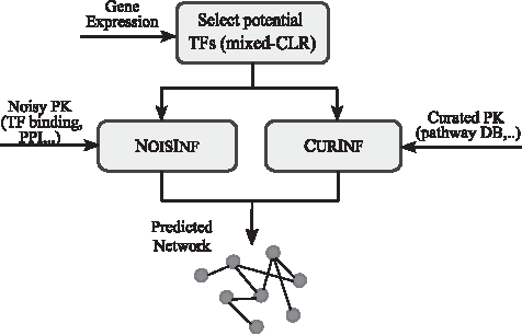end{document} 's using the Inferelator algorithm, which uses elastic net (Bonneau et al., 2006). We integrate PK into the model using either NoisInf for a noisy prior or CurInf for a reliable PK in the fine-grain step. PEAK inference system is highlighted in Figure 1.

FIG. 1.

PEAK GRN inference system. Gene expression data are fed into the system, along with optionally other data such as TF binding or pathways. Potential TFs are extracted, then based on the PK, either NoisInf or CurInf is applied. GRN, gene regulatory network; PK, prior knowledge; TF, transcription factor.

2.2.1. Coarse-grain prediction using mixed CLR

The purpose of this step is to find a subset of potential regulators P_i for each response gene y_i. Instead of considering all N genes as potential regulators in the regression model for gene y_i, only a small subset is included. Using a constant number of TFs per gene reduces the complexity of the regression model and improves prediction. This filtering is done using mixed CLR (context likelihood estimator) proposed in Madar et al. (2010). To find the set P_i, first mutual information (MI) is calculated to measure the dependence between every pair of genes. Second, mixed CLR is used as a background correction method to find the significance of the calculated MI between TF and its target gene. Finally, for each target gene, TFs with the highest mixed-CLR scores are chosen as the set of likely regulators P_i, which will be considered in the fine-grain prediction. The cutoff for the top regulators is a parameter, and it was chosen to be 30 TFs per gene as in Greenfield et al. (2013). The cutoff is a tuning parameter that can be chosen according to the biological relevance of the data, that is, an estimated upper bound on the number of TFs that are expected to regulate each gene.

2.2.2. Fine-grain prediction using elastic net

After choosing a set P_i of potential regulators for each gene using mixed CLR, the next step is to solve the ODE regression model to find the unknown coefficients. We use elastic net to find the final set of predicted regulators for each gene as in Greenfield et al. (2013). Elastic net is used to solve the regression model for each gene by performing variable selection. The magnitude of the coefficient, \documentclass{aastex}\usepackage{amsbsy}\usepackage{amsfonts}\usepackage{amssymb}\usepackage{bm}\usepackage{mathrsfs}\usepackage{pifont}\usepackage{stmaryrd}\usepackage{textcomp}\usepackage{portland, xspace}\usepackage{amsmath, amsxtra}\usepackage{upgreek}\pagestyle{empty}\DeclareMathSizes{10}{9}{7}{6}\begin{document} $$\vert { \beta _{i , p}} \vert$$ \end{document} , is considered the confidence of the regulatory relation between genes y_i and x_p.

For each gene y_i, it is required to solve the following linear regression model to find the unknown \documentclass{aastex}\usepackage{amsbsy}\usepackage{amsfonts}\usepackage{amssymb}\usepackage{bm}\usepackage{mathrsfs}\usepackage{pifont}\usepackage{stmaryrd}\usepackage{textcomp}\usepackage{portland, xspace}\usepackage{amsmath, amsxtra}\usepackage{upgreek}\pagestyle{empty}\DeclareMathSizes{10}{9}{7}{6}\begin{document} $${ \beta _{i , p}}$$ \end{document} 's \documentclass{aastex}\usepackage{amsbsy}\usepackage{amsfonts}\usepackage{amssymb}\usepackage{bm}\usepackage{mathrsfs}\usepackage{pifont}\usepackage{stmaryrd}\usepackage{textcomp}\usepackage{portland, xspace}\usepackage{amsmath, amsxtra}\usepackage{upgreek}\pagestyle{empty}\DeclareMathSizes{10}{9}{7}{6}\begin{document} \begin{align*} {y_i} ( r ) = \mathop \sum \limits_{p \in {P_i}} { \beta _{i , p}}{x_p} ( r ), \tag{5} \end{align*} \end{document}

where r spans all available expression data, including time-series and steady state observations. Ordinary least squares (OLS) is a popular method to estimate these \documentclass{aastex}\usepackage{amsbsy}\usepackage{amsfonts}\usepackage{amssymb}\usepackage{bm}\usepackage{mathrsfs}\usepackage{pifont}\usepackage{stmaryrd}\usepackage{textcomp}\usepackage{portland, xspace}\usepackage{amsmath, amsxtra}\usepackage{upgreek}\pagestyle{empty}\DeclareMathSizes{10}{9}{7}{6}\begin{document} $${ \beta _{i , p}}$$ \end{document} 's from training data. In general, this is obtained by minimizing the prediction error, which is the sum of squares of the residuals between the predicted value (from Equation (5)) and the actual observed value \documentclass{aastex}\usepackage{amsbsy}\usepackage{amsfonts}\usepackage{amssymb}\usepackage{bm}\usepackage{mathrsfs}\usepackage{pifont}\usepackage{stmaryrd}\usepackage{textcomp}\usepackage{portland, xspace}\usepackage{amsmath, amsxtra}\usepackage{upgreek}\pagestyle{empty}\DeclareMathSizes{10}{9}{7}{6}\begin{document} $${y_i} ( r )$$ \end{document} . This can be written as an objective function to minimize \documentclass{aastex}\usepackage{amsbsy}\usepackage{amsfonts}\usepackage{amssymb}\usepackage{bm}\usepackage{mathrsfs}\usepackage{pifont}\usepackage{stmaryrd}\usepackage{textcomp}\usepackage{portland, xspace}\usepackage{amsmath, amsxtra}\usepackage{upgreek}\pagestyle{empty}\DeclareMathSizes{10}{9}{7}{6}\begin{document} \begin{align*} E ( { \beta _i} ) = \mathop \sum \limits_{r = 1}^R { \left\vert {{y_i} ( r ) - \mathop \sum \limits_{p \in {P_i}} { \beta _{i , p}}{x_p} ( r ) } \right\vert ^2}. \tag{6} \end{align*} \end{document}

The estimated \documentclass{aastex}\usepackage{amsbsy}\usepackage{amsfonts}\usepackage{amssymb}\usepackage{bm}\usepackage{mathrsfs}\usepackage{pifont}\usepackage{stmaryrd}\usepackage{textcomp}\usepackage{portland, xspace}\usepackage{amsmath, amsxtra}\usepackage{upgreek}\pagestyle{empty}\DeclareMathSizes{10}{9}{7}{6}\begin{document} $${ \beta _{i , p}}$$ \end{document} 's using the OLS method has the limitation of producing a nonsparse solution. In the case of GRN inference, we would like to select a subset of the TFs that regulate the target gene, and expect most of the other \documentclass{aastex}\usepackage{amsbsy}\usepackage{amsfonts}\usepackage{amssymb}\usepackage{bm}\usepackage{mathrsfs}\usepackage{pifont}\usepackage{stmaryrd}\usepackage{textcomp}\usepackage{portland, xspace}\usepackage{amsmath, amsxtra}\usepackage{upgreek}\pagestyle{empty}\DeclareMathSizes{10}{9}{7}{6}\begin{document} $${ \beta _{i , p}}$$ \end{document} 's to be 0's, that is, we want to select a sparse model. Several methods, called regularization methods, exist to find a sparse model, such as lasso, ridge, and elastic net (Zou and Hastie, 2005). Elastic net was shown to be more suitable than other regularization methods when a correlation exists between predictors. In a biological context, correlation between the expression levels of TFs is common, and thus elastic net is preferred in solving gene regulation models (Zou and Hastie, 2005). Elastic net adds a constraint (or a penalty) \documentclass{aastex}\usepackage{amsbsy}\usepackage{amsfonts}\usepackage{amssymb}\usepackage{bm}\usepackage{mathrsfs}\usepackage{pifont}\usepackage{stmaryrd}\usepackage{textcomp}\usepackage{portland, xspace}\usepackage{amsmath, amsxtra}\usepackage{upgreek}\pagestyle{empty}\DeclareMathSizes{10}{9}{7}{6}\begin{document} $$C ( { \beta _i} )$$ \end{document} to the objective function in Equation (6) to limit the number of variables included in the equation by forcing their sum to be less than a certain value. The elastic net penalty is a combination of L \documentclass{aastex}\usepackage{amsbsy}\usepackage{amsfonts}\usepackage{amssymb}\usepackage{bm}\usepackage{mathrsfs}\usepackage{pifont}\usepackage{stmaryrd}\usepackage{textcomp}\usepackage{portland, xspace}\usepackage{amsmath, amsxtra}\usepackage{upgreek}\pagestyle{empty}\DeclareMathSizes{10}{9}{7}{6}\begin{document} $$_1$$ \end{document} -norm and L \documentclass{aastex}\usepackage{amsbsy}\usepackage{amsfonts}\usepackage{amssymb}\usepackage{bm}\usepackage{mathrsfs}\usepackage{pifont}\usepackage{stmaryrd}\usepackage{textcomp}\usepackage{portland, xspace}\usepackage{amsmath, amsxtra}\usepackage{upgreek}\pagestyle{empty}\DeclareMathSizes{10}{9}{7}{6}\begin{document} $$_2$$ \end{document} -norm penalties. The elastic net objective function is given by \documentclass{aastex}\usepackage{amsbsy}\usepackage{amsfonts}\usepackage{amssymb}\usepackage{bm}\usepackage{mathrsfs}\usepackage{pifont}\usepackage{stmaryrd}\usepackage{textcomp}\usepackage{portland, xspace}\usepackage{amsmath, amsxtra}\usepackage{upgreek}\pagestyle{empty}\DeclareMathSizes{10}{9}{7}{6}\begin{document} \begin{align*} \begin{matrix} {J ( { \beta _i} ) } \hfill & { = E ( { \beta _i} ) + \alpha C ( { \beta _i} ),} \hfill \\ {} \hfill & {} \hfill \\ \end{matrix} \tag{7} \end{align*} \end{document}

2.3. Adding PK

We differentiate between two types of PK: curated and noisy. Regulatory relations from experimentally verified pathways are considered curated or reliable PK. Noisy or unreliable resources can be derived from PPI networks, physical binding, interactions mapped from homologous genes, or hypothesized relations. We propose a GRN inference method that we call CurInf for reliable PK, and we use the method MEN, proposed in Greenfield et al. (2013), to incorporate noisy PK.

2.3.1. NoisInf for noisy PK

Greenfield et al. (2013) proposed MEN, a robust method for adding noisy PK to GRN prediction. MEN scales the elastic net penalty to integrate PK about the topology of the GRN based on adaptive elastic net (Zou and Zhang, 2009). In NoisInf, the penalty term in Equation (8) is modified by using different degrees of shrinkage on the coefficients \documentclass{aastex}\usepackage{amsbsy}\usepackage{amsfonts}\usepackage{amssymb}\usepackage{bm}\usepackage{mathrsfs}\usepackage{pifont}\usepackage{stmaryrd}\usepackage{textcomp}\usepackage{portland, xspace}\usepackage{amsmath, amsxtra}\usepackage{upgreek}\pagestyle{empty}\DeclareMathSizes{10}{9}{7}{6}\begin{document} $${ \beta _{i , p}}$$ \end{document} for different predictors. This is done by multiplying the L \documentclass{aastex}\usepackage{amsbsy}\usepackage{amsfonts}\usepackage{amssymb}\usepackage{bm}\usepackage{mathrsfs}\usepackage{pifont}\usepackage{stmaryrd}\usepackage{textcomp}\usepackage{portland, xspace}\usepackage{amsmath, amsxtra}\usepackage{upgreek}\pagestyle{empty}\DeclareMathSizes{10}{9}{7}{6}\begin{document} $$_1$$ \end{document} term by small values, denoted \documentclass{aastex}\usepackage{amsbsy}\usepackage{amsfonts}\usepackage{amssymb}\usepackage{bm}\usepackage{mathrsfs}\usepackage{pifont}\usepackage{stmaryrd}\usepackage{textcomp}\usepackage{portland, xspace}\usepackage{amsmath, amsxtra}\usepackage{upgreek}\pagestyle{empty}\DeclareMathSizes{10}{9}{7}{6}\begin{document} $${ \theta _{i , p}}$$ \end{document} , to prevent shrinkage on the parameter \documentclass{aastex}\usepackage{amsbsy}\usepackage{amsfonts}\usepackage{amssymb}\usepackage{bm}\usepackage{mathrsfs}\usepackage{pifont}\usepackage{stmaryrd}\usepackage{textcomp}\usepackage{portland, xspace}\usepackage{amsmath, amsxtra}\usepackage{upgreek}\pagestyle{empty}\DeclareMathSizes{10}{9}{7}{6}\begin{document} $${ \beta _{i , p}}$$ \end{document} if the corresponding TF x_p is known to be a true regulator of the target gene y_i. Adding PK in this way tolerates noise and accepts prior information only if it is supported by the gene expression data.

We follow the MEN's main approach (Greenfield et al., 2013) for integrating noisy PK. Each response gene y_i has a PK vector \documentclass{aastex}\usepackage{amsbsy}\usepackage{amsfonts}\usepackage{amssymb}\usepackage{bm}\usepackage{mathrsfs}\usepackage{pifont}\usepackage{stmaryrd}\usepackage{textcomp}\usepackage{portland, xspace}\usepackage{amsmath, amsxtra}\usepackage{upgreek}\pagestyle{empty}\DeclareMathSizes{10}{9}{7}{6}\begin{document} $${ \Theta _i}$$ \end{document} , where \documentclass{aastex}\usepackage{amsbsy}\usepackage{amsfonts}\usepackage{amssymb}\usepackage{bm}\usepackage{mathrsfs}\usepackage{pifont}\usepackage{stmaryrd}\usepackage{textcomp}\usepackage{portland, xspace}\usepackage{amsmath, amsxtra}\usepackage{upgreek}\pagestyle{empty}\DeclareMathSizes{10}{9}{7}{6}\begin{document} $${ \theta _{i , p}}$$ \end{document} equals 1 if no PK exists between gene y_i and TF x_p and \documentclass{aastex}\usepackage{amsbsy}\usepackage{amsfonts}\usepackage{amssymb}\usepackage{bm}\usepackage{mathrsfs}\usepackage{pifont}\usepackage{stmaryrd}\usepackage{textcomp}\usepackage{portland, xspace}\usepackage{amsmath, amsxtra}\usepackage{upgreek}\pagestyle{empty}\DeclareMathSizes{10}{9}{7}{6}\begin{document} $$< 1$$ \end{document} if PK exists (i.e., there is a lower constraint on its corresponding coefficient). The weight \documentclass{aastex}\usepackage{amsbsy}\usepackage{amsfonts}\usepackage{amssymb}\usepackage{bm}\usepackage{mathrsfs}\usepackage{pifont}\usepackage{stmaryrd}\usepackage{textcomp}\usepackage{portland, xspace}\usepackage{amsmath, amsxtra}\usepackage{upgreek}\pagestyle{empty}\DeclareMathSizes{10}{9}{7}{6}\begin{document} $${ \theta _{i , p}}$$ \end{document} can be varied according to the amount of confidence in the prior information. The objective function Equation (7) in the case of noisy prior using NoisInf is \documentclass{aastex}\usepackage{amsbsy}\usepackage{amsfonts}\usepackage{amssymb}\usepackage{bm}\usepackage{mathrsfs}\usepackage{pifont}\usepackage{stmaryrd}\usepackage{textcomp}\usepackage{portland, xspace}\usepackage{amsmath, amsxtra}\usepackage{upgreek}\pagestyle{empty}\DeclareMathSizes{10}{9}{7}{6}\begin{document} \begin{align*} \begin{matrix} {J ( { \beta _i} ) = E ( { \beta _i} ) + \alpha \lambda \mathop \sum \limits_{p \in {P_i}} \vert { \theta _{i , p}}{ \beta _{i , p}} \vert + \alpha ( 1 - \lambda ) \mathop \sum \limits_{p \in {P_i}} \beta _{i , p}^2.} \hfill \\ \end{matrix} \tag{9} \end{align*} \end{document}

2.3.2. CurInf for reliable PK

NoisInf adds PK by reducing the penalty term of predictors that are thought to be true TFs of the gene. NoisInf cannot predict a regulatory relation if it is not supported by the gene expression data, because it will be considered noise. In some cases, curated PK can be unsupported by the gene expression data. For example, if the expression data are noisy or the experimental design did not capture a clear causality relation between the gene and the TF, then the TF will not be predicted as a regulator for that gene even with no penalty term in the objective function Equation (9).

We propose a method to add reliable PK, even if it is not supported by the gene expression data. CurInf adds the PK to the main error term \documentclass{aastex}\usepackage{amsbsy}\usepackage{amsfonts}\usepackage{amssymb}\usepackage{bm}\usepackage{mathrsfs}\usepackage{pifont}\usepackage{stmaryrd}\usepackage{textcomp}\usepackage{portland, xspace}\usepackage{amsmath, amsxtra}\usepackage{upgreek}\pagestyle{empty}\DeclareMathSizes{10}{9}{7}{6}\begin{document} $$E ( { \beta _i} )$$ \end{document} of the objective function Equation (7) rather than in the penalty term \documentclass{aastex}\usepackage{amsbsy}\usepackage{amsfonts}\usepackage{amssymb}\usepackage{bm}\usepackage{mathrsfs}\usepackage{pifont}\usepackage{stmaryrd}\usepackage{textcomp}\usepackage{portland, xspace}\usepackage{amsmath, amsxtra}\usepackage{upgreek}\pagestyle{empty}\DeclareMathSizes{10}{9}{7}{6}\begin{document} $$C ( { \beta _i} )$$ \end{document} . The features of the design matrix of response gene y_i is scaled using the PK vector \documentclass{aastex}\usepackage{amsbsy}\usepackage{amsfonts}\usepackage{amssymb}\usepackage{bm}\usepackage{mathrsfs}\usepackage{pifont}\usepackage{stmaryrd}\usepackage{textcomp}\usepackage{portland, xspace}\usepackage{amsmath, amsxtra}\usepackage{upgreek}\pagestyle{empty}\DeclareMathSizes{10}{9}{7}{6}\begin{document} $${ \Theta _i}$$ \end{document} , where \documentclass{aastex}\usepackage{amsbsy}\usepackage{amsfonts}\usepackage{amssymb}\usepackage{bm}\usepackage{mathrsfs}\usepackage{pifont}\usepackage{stmaryrd}\usepackage{textcomp}\usepackage{portland, xspace}\usepackage{amsmath, amsxtra}\usepackage{upgreek}\pagestyle{empty}\DeclareMathSizes{10}{9}{7}{6}\begin{document} $${ \theta _{i , p}}$$ \end{document} equals 1 if no PK exists between gene y_i and TF x_p and \documentclass{aastex}\usepackage{amsbsy}\usepackage{amsfonts}\usepackage{amssymb}\usepackage{bm}\usepackage{mathrsfs}\usepackage{pifont}\usepackage{stmaryrd}\usepackage{textcomp}\usepackage{portland, xspace}\usepackage{amsmath, amsxtra}\usepackage{upgreek}\pagestyle{empty}\DeclareMathSizes{10}{9}{7}{6}\begin{document} $$< 1$$ \end{document} if PK exists. The motivation is that, in regularized linear models, features that have orders of magnitude higher variance can dominate the objective function. Thus, scaling the features causes known TFs to have a relatively higher variance that will favor their selection when solving the model. The objective function Equation (7) after CurInf becomes \documentclass{aastex}\usepackage{amsbsy}\usepackage{amsfonts}\usepackage{amssymb}\usepackage{bm}\usepackage{mathrsfs}\usepackage{pifont}\usepackage{stmaryrd}\usepackage{textcomp}\usepackage{portland, xspace}\usepackage{amsmath, amsxtra}\usepackage{upgreek}\pagestyle{empty}\DeclareMathSizes{10}{9}{7}{6}\begin{document} \begin{align*} \begin{matrix} {J ( { \beta _i} ) = } { \mathop \sum \limits_{r = 1}^R {{ \left\vert {{y_i} ( r ) - \mathop \sum \limits_{p \in {P_i}} { \beta _{i , p}} \theta _{i , p}^{ - 1}{x_p} ( r ) } \right\vert }^2} + \alpha C ( { \beta _i} ).} \hfill \\ \end{matrix} \tag{10} \end{align*} \end{document}

The term \documentclass{aastex}\usepackage{amsbsy}\usepackage{amsfonts}\usepackage{amssymb}\usepackage{bm}\usepackage{mathrsfs}\usepackage{pifont}\usepackage{stmaryrd}\usepackage{textcomp}\usepackage{portland, xspace}\usepackage{amsmath, amsxtra}\usepackage{upgreek}\pagestyle{empty}\DeclareMathSizes{10}{9}{7}{6}\begin{document} $$\theta _{i , p}^{ - 1}{x_p} ( r )$$ \end{document} means dividing all the expression levels of predictor x_p by the PK term \documentclass{aastex}\usepackage{amsbsy}\usepackage{amsfonts}\usepackage{amssymb}\usepackage{bm}\usepackage{mathrsfs}\usepackage{pifont}\usepackage{stmaryrd}\usepackage{textcomp}\usepackage{portland, xspace}\usepackage{amsmath, amsxtra}\usepackage{upgreek}\pagestyle{empty}\DeclareMathSizes{10}{9}{7}{6}\begin{document} $${ \theta _{i , p}}$$ \end{document} that corresponds to its relation with gene y_i. For example, if x_p is known to be a TF for y_i, then \documentclass{aastex}\usepackage{amsbsy}\usepackage{amsfonts}\usepackage{amssymb}\usepackage{bm}\usepackage{mathrsfs}\usepackage{pifont}\usepackage{stmaryrd}\usepackage{textcomp}\usepackage{portland, xspace}\usepackage{amsmath, amsxtra}\usepackage{upgreek}\pagestyle{empty}\DeclareMathSizes{10}{9}{7}{6}\begin{document} $${ \theta _{i , p}}$$ \end{document} will have a small value. This results in upscaling the term \documentclass{aastex}\usepackage{amsbsy}\usepackage{amsfonts}\usepackage{amssymb}\usepackage{bm}\usepackage{mathrsfs}\usepackage{pifont}\usepackage{stmaryrd}\usepackage{textcomp}\usepackage{portland, xspace}\usepackage{amsmath, amsxtra}\usepackage{upgreek}\pagestyle{empty}\DeclareMathSizes{10}{9}{7}{6}\begin{document} $$\theta _{i , p}^{ - 1}{x_p} ( r )$$ \end{document} . If no PK exists, \documentclass{aastex}\usepackage{amsbsy}\usepackage{amsfonts}\usepackage{amssymb}\usepackage{bm}\usepackage{mathrsfs}\usepackage{pifont}\usepackage{stmaryrd}\usepackage{textcomp}\usepackage{portland, xspace}\usepackage{amsmath, amsxtra}\usepackage{upgreek}\pagestyle{empty}\DeclareMathSizes{10}{9}{7}{6}\begin{document} $${ \theta _{i , p}}$$ \end{document} equals 1, and its expression values \documentclass{aastex}\usepackage{amsbsy}\usepackage{amsfonts}\usepackage{amssymb}\usepackage{bm}\usepackage{mathrsfs}\usepackage{pifont}\usepackage{stmaryrd}\usepackage{textcomp}\usepackage{portland, xspace}\usepackage{amsmath, amsxtra}\usepackage{upgreek}\pagestyle{empty}\DeclareMathSizes{10}{9}{7}{6}\begin{document} $${x_p} ( r )$$ \end{document} are not scaled. We choose to divide by small values \documentclass{aastex}\usepackage{amsbsy}\usepackage{amsfonts}\usepackage{amssymb}\usepackage{bm}\usepackage{mathrsfs}\usepackage{pifont}\usepackage{stmaryrd}\usepackage{textcomp}\usepackage{portland, xspace}\usepackage{amsmath, amsxtra}\usepackage{upgreek}\pagestyle{empty}\DeclareMathSizes{10}{9}{7}{6}\begin{document} $${ \theta _{i , p}}$$ \end{document} instead of multiplying by larger values to be consistent with the NoisInf notation described earlier.

Coordinate descent (Friedman et al., 2010) is used for an efficient iterative implementation of elastic net, which is proposed in Zou and Hastie (2005). CV is used to find regularization of the parameters \documentclass{aastex}\usepackage{amsbsy}\usepackage{amsfonts}\usepackage{amssymb}\usepackage{bm}\usepackage{mathrsfs}\usepackage{pifont}\usepackage{stmaryrd}\usepackage{textcomp}\usepackage{portland, xspace}\usepackage{amsmath, amsxtra}\usepackage{upgreek}\pagestyle{empty}\DeclareMathSizes{10}{9}{7}{6}\begin{document} $$\alpha$$ \end{document} and \documentclass{aastex}\usepackage{amsbsy}\usepackage{amsfonts}\usepackage{amssymb}\usepackage{bm}\usepackage{mathrsfs}\usepackage{pifont}\usepackage{stmaryrd}\usepackage{textcomp}\usepackage{portland, xspace}\usepackage{amsmath, amsxtra}\usepackage{upgreek}\pagestyle{empty}\DeclareMathSizes{10}{9}{7}{6}\begin{document} $$\lambda$$ \end{document} because they are difficult to choose. CurInf and NoisInf are sensitive to the choice of these parameters, which greatly affects the prediction accuracy. We propose a heuristic to bound the search range of the regularization parameters.

2.4. Bounded CV for choosing model parameters

CurInf: As CurInf integrates PK using the error term \documentclass{aastex}\usepackage{amsbsy}\usepackage{amsfonts}\usepackage{amssymb}\usepackage{bm}\usepackage{mathrsfs}\usepackage{pifont}\usepackage{stmaryrd}\usepackage{textcomp}\usepackage{portland, xspace}\usepackage{amsmath, amsxtra}\usepackage{upgreek}\pagestyle{empty}\DeclareMathSizes{10}{9}{7}{6}\begin{document} $$E ( { \beta _i} )$$ \end{document} not the penalty term \documentclass{aastex}\usepackage{amsbsy}\usepackage{amsfonts}\usepackage{amssymb}\usepackage{bm}\usepackage{mathrsfs}\usepackage{pifont}\usepackage{stmaryrd}\usepackage{textcomp}\usepackage{portland, xspace}\usepackage{amsmath, amsxtra}\usepackage{upgreek}\pagestyle{empty}\DeclareMathSizes{10}{9}{7}{6}\begin{document} $$C ( { \beta _i} )$$ \end{document} in Equation (7), less weight should be given to the penalty term. The penalty term weight \documentclass{aastex}\usepackage{amsbsy}\usepackage{amsfonts}\usepackage{amssymb}\usepackage{bm}\usepackage{mathrsfs}\usepackage{pifont}\usepackage{stmaryrd}\usepackage{textcomp}\usepackage{portland, xspace}\usepackage{amsmath, amsxtra}\usepackage{upgreek}\pagestyle{empty}\DeclareMathSizes{10}{9}{7}{6}\begin{document} $$\alpha$$ \end{document} is chosen using CV. We provide a bounded search range for the CV consisting of small numbers (from \documentclass{aastex}\usepackage{amsbsy}\usepackage{amsfonts}\usepackage{amssymb}\usepackage{bm}\usepackage{mathrsfs}\usepackage{pifont}\usepackage{stmaryrd}\usepackage{textcomp}\usepackage{portland, xspace}\usepackage{amsmath, amsxtra}\usepackage{upgreek}\pagestyle{empty}\DeclareMathSizes{10}{9}{7}{6}\begin{document} $$0.001$$ \end{document} to \documentclass{aastex}\usepackage{amsbsy}\usepackage{amsfonts}\usepackage{amssymb}\usepackage{bm}\usepackage{mathrsfs}\usepackage{pifont}\usepackage{stmaryrd}\usepackage{textcomp}\usepackage{portland, xspace}\usepackage{amsmath, amsxtra}\usepackage{upgreek}\pagestyle{empty}\DeclareMathSizes{10}{9}{7}{6}\begin{document} $$0.1$$ \end{document} ) for all data sets.

NoisInf: In contrast, NoisInf uses the penalty term \documentclass{aastex}\usepackage{amsbsy}\usepackage{amsfonts}\usepackage{amssymb}\usepackage{bm}\usepackage{mathrsfs}\usepackage{pifont}\usepackage{stmaryrd}\usepackage{textcomp}\usepackage{portland, xspace}\usepackage{amsmath, amsxtra}\usepackage{upgreek}\pagestyle{empty}\DeclareMathSizes{10}{9}{7}{6}\begin{document} $$C ( { \beta _i} )$$ \end{document} to incorporate PK; thus it needs more weight for the penalty term to emphasize PK. In this case, NoisInf needs a range of higher values for \documentclass{aastex}\usepackage{amsbsy}\usepackage{amsfonts}\usepackage{amssymb}\usepackage{bm}\usepackage{mathrsfs}\usepackage{pifont}\usepackage{stmaryrd}\usepackage{textcomp}\usepackage{portland, xspace}\usepackage{amsmath, amsxtra}\usepackage{upgreek}\pagestyle{empty}\DeclareMathSizes{10}{9}{7}{6}\begin{document} $$\alpha$$ \end{document} in the CV.

Experimental results show that this strategy is successful in increasing the chance of PK integration into the selected model, which results in a higher accuracy. Also, based on test results, the balancing parameter between L \documentclass{aastex}\usepackage{amsbsy}\usepackage{amsfonts}\usepackage{amssymb}\usepackage{bm}\usepackage{mathrsfs}\usepackage{pifont}\usepackage{stmaryrd}\usepackage{textcomp}\usepackage{portland, xspace}\usepackage{amsmath, amsxtra}\usepackage{upgreek}\pagestyle{empty}\DeclareMathSizes{10}{9}{7}{6}\begin{document} $$_1$$ \end{document} -norm and L \documentclass{aastex}\usepackage{amsbsy}\usepackage{amsfonts}\usepackage{amssymb}\usepackage{bm}\usepackage{mathrsfs}\usepackage{pifont}\usepackage{stmaryrd}\usepackage{textcomp}\usepackage{portland, xspace}\usepackage{amsmath, amsxtra}\usepackage{upgreek}\pagestyle{empty}\DeclareMathSizes{10}{9}{7}{6}\begin{document} $$_2$$ \end{document} -norm, \documentclass{aastex}\usepackage{amsbsy}\usepackage{amsfonts}\usepackage{amssymb}\usepackage{bm}\usepackage{mathrsfs}\usepackage{pifont}\usepackage{stmaryrd}\usepackage{textcomp}\usepackage{portland, xspace}\usepackage{amsmath, amsxtra}\usepackage{upgreek}\pagestyle{empty}\DeclareMathSizes{10}{9}{7}{6}\begin{document} $$\lambda$$ \end{document} , has minimal effect compared with \documentclass{aastex}\usepackage{amsbsy}\usepackage{amsfonts}\usepackage{amssymb}\usepackage{bm}\usepackage{mathrsfs}\usepackage{pifont}\usepackage{stmaryrd}\usepackage{textcomp}\usepackage{portland, xspace}\usepackage{amsmath, amsxtra}\usepackage{upgreek}\pagestyle{empty}\DeclareMathSizes{10}{9}{7}{6}\begin{document} $$\alpha$$ \end{document} . Thus \documentclass{aastex}\usepackage{amsbsy}\usepackage{amsfonts}\usepackage{amssymb}\usepackage{bm}\usepackage{mathrsfs}\usepackage{pifont}\usepackage{stmaryrd}\usepackage{textcomp}\usepackage{portland, xspace}\usepackage{amsmath, amsxtra}\usepackage{upgreek}\pagestyle{empty}\DeclareMathSizes{10}{9}{7}{6}\begin{document} $$\lambda$$ \end{document} is chosen to be \documentclass{aastex}\usepackage{amsbsy}\usepackage{amsfonts}\usepackage{amssymb}\usepackage{bm}\usepackage{mathrsfs}\usepackage{pifont}\usepackage{stmaryrd}\usepackage{textcomp}\usepackage{portland, xspace}\usepackage{amsmath, amsxtra}\usepackage{upgreek}\pagestyle{empty}\DeclareMathSizes{10}{9}{7}{6}\begin{document} $$0.5$$ \end{document} , giving equal weight to the L \documentclass{aastex}\usepackage{amsbsy}\usepackage{amsfonts}\usepackage{amssymb}\usepackage{bm}\usepackage{mathrsfs}\usepackage{pifont}\usepackage{stmaryrd}\usepackage{textcomp}\usepackage{portland, xspace}\usepackage{amsmath, amsxtra}\usepackage{upgreek}\pagestyle{empty}\DeclareMathSizes{10}{9}{7}{6}\begin{document} $$_1$$ \end{document} -norm and the L \documentclass{aastex}\usepackage{amsbsy}\usepackage{amsfonts}\usepackage{amssymb}\usepackage{bm}\usepackage{mathrsfs}\usepackage{pifont}\usepackage{stmaryrd}\usepackage{textcomp}\usepackage{portland, xspace}\usepackage{amsmath, amsxtra}\usepackage{upgreek}\pagestyle{empty}\DeclareMathSizes{10}{9}{7}{6}\begin{document} $$_2$$ \end{document} -norm.

3. Results

3.1. Data sets

For testing and analysis of the GRN inference using PK, we used three data sets from the DREAM5 benchmark (Marbach et al., 2012), summarized in Table 1. The chosen benchmark has gold standard GRNs (TF–target interactions) available for each data set to validate predicted networks. Although predicted interactions not in the gold standard are considered false positives, many can be true interactions, because the gold standard is stringent and incomplete. Each data set consists of gene expression data for N genes in R experiments. Each experiment can have a description whether it is time series or steady state, time (if applicable), and experiment repetition information. A list of candidate TFs is provided in the benchmark for each data set.

Table 1.

Data Sets Used for Training and Testing

Data set	Samples	Genes	TFs	Edges in gold standard
In silico (DREAM5)	805	1643	195	4012
Escherichia coli	805	1100	178	2066
Saccharomyces cerevisiae	536	5950	333	3940

TF, transcription factor.

The first data set is a synthetic network generated by the DREAM5 organizers. The second data set comes from the prokaryotic model organism E. coli, which has a well-studied GRN. The raw expression data were downloaded from the GEO database. The gold standard GRN was extracted from the curated database RegulonDB version 7 (Gama-Castro et al., 2016). We use a subset of the E. coli genes, in which each gene has at least one interaction in the gold standard. The third data set comes from the eukaryotic model organism S. cerevisiae. Normalization of the microarray data was done using robust multichip averaging (Bolstad et al., 2003).

We use area under precision-recall curve (AUPR) as the measure of performance as adapted in Greenfield et al. (2013) and Marbach et al. (2012). AUPR is more suitable than the receiver operating characteristic in applications, where the number of positive and negative samples is unbalanced. In GRNs, the network is expected to be sparse, that is, nonedges are significantly higher than existing edges.

3.2. Better integration of curated PK

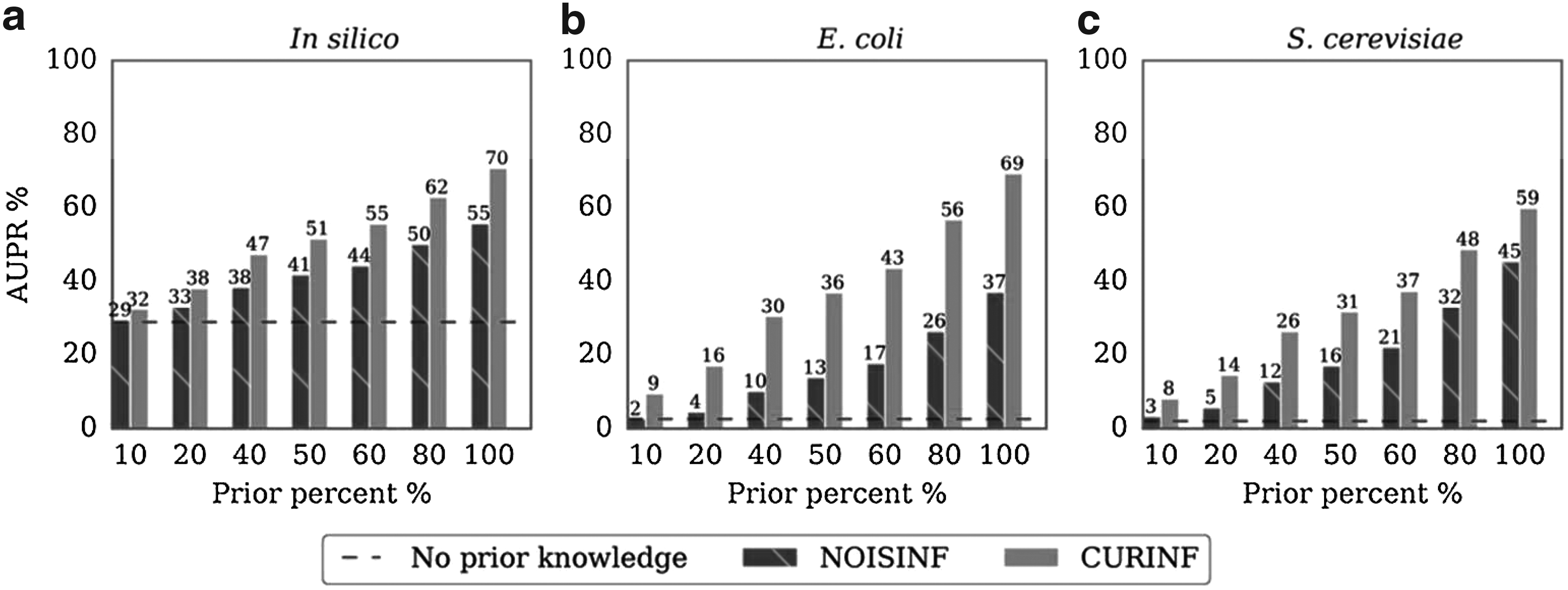
We compared the ability of CurInf and NoisInf to incorporate curated PK to the inference algorithm. Incremental percentages of the gold standard edges are added to NoisInf and CurInf as curated PK, then the AUPR is calculated for the reconstructed GRNs. Figure 2 shows the accuracy measure AUPR for NoisInf and CurInf on the three data sets. In both methods, the accuracy increases as the PK percentage increases, which is significantly higher than any method without PK tested in the DREAM benchmark (Supplementary Fig. S1).

FIG. 2.

The ability of NoisInf and CurInf inference methods to incorporate curated PK. Different percentages of the gold standard edges are used as PK to the inference algorithm, and the resulting networks are evaluated for (a) In silico, (b) E. coli, and (c) S. cerevisiae. The dotted lines represent the accuracy without using any PK.

CurInf is superior to NoisInf in the integration of curated PK, resulting in higher accuracy GRN, as shown in Figure 2. The difference is more prominent in the E. coli and S. cerevisiae data than in the synthetic data. When adding \documentclass{aastex}\usepackage{amsbsy}\usepackage{amsfonts}\usepackage{amssymb}\usepackage{bm}\usepackage{mathrsfs}\usepackage{pifont}\usepackage{stmaryrd}\usepackage{textcomp}\usepackage{portland, xspace}\usepackage{amsmath, amsxtra}\usepackage{upgreek}\pagestyle{empty}\DeclareMathSizes{10}{9}{7}{6}\begin{document} $$100 \%$$ \end{document} of the gold standard as curated PK, CurInf was able to improve the AUPR score over NoisInf by \documentclass{aastex}\usepackage{amsbsy}\usepackage{amsfonts}\usepackage{amssymb}\usepackage{bm}\usepackage{mathrsfs}\usepackage{pifont}\usepackage{stmaryrd}\usepackage{textcomp}\usepackage{portland, xspace}\usepackage{amsmath, amsxtra}\usepackage{upgreek}\pagestyle{empty}\DeclareMathSizes{10}{9}{7}{6}\begin{document} $$27.3 \%$$ \end{document} in synthetic data, \documentclass{aastex}\usepackage{amsbsy}\usepackage{amsfonts}\usepackage{amssymb}\usepackage{bm}\usepackage{mathrsfs}\usepackage{pifont}\usepackage{stmaryrd}\usepackage{textcomp}\usepackage{portland, xspace}\usepackage{amsmath, amsxtra}\usepackage{upgreek}\pagestyle{empty}\DeclareMathSizes{10}{9}{7}{6}\begin{document} $$86.5 \%$$ \end{document} in E. coli data, and \documentclass{aastex}\usepackage{amsbsy}\usepackage{amsfonts}\usepackage{amssymb}\usepackage{bm}\usepackage{mathrsfs}\usepackage{pifont}\usepackage{stmaryrd}\usepackage{textcomp}\usepackage{portland, xspace}\usepackage{amsmath, amsxtra}\usepackage{upgreek}\pagestyle{empty}\DeclareMathSizes{10}{9}{7}{6}\begin{document} $$31.1 \%$$ \end{document} in S. cerevisiae data.

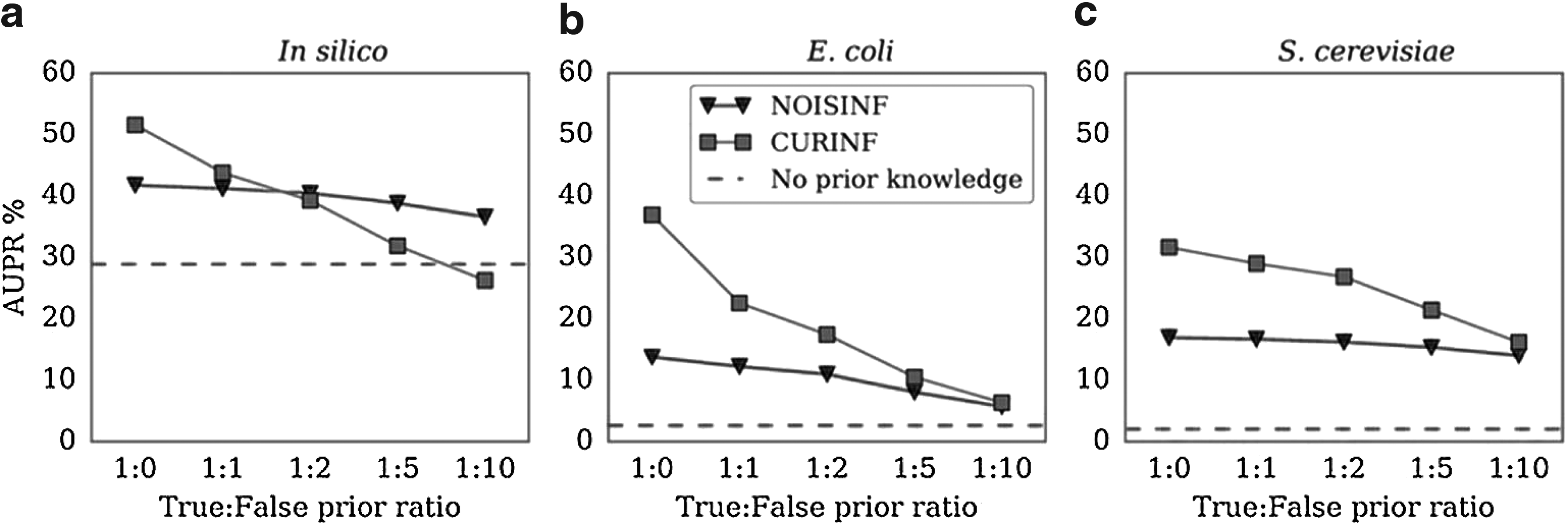
3.3. Tolerance to noisy PK

PEAK uses NoisInf scaling to integrate PK when it is believed to be noisy. We tested adding noisy PK to CurInf and NoisInf, and, as expected, NoisInf is more robust and thus more suitable to use with noisy PK. In Figure 3, we added different ratios of true to false PK. True PK is \documentclass{aastex}\usepackage{amsbsy}\usepackage{amsfonts}\usepackage{amssymb}\usepackage{bm}\usepackage{mathrsfs}\usepackage{pifont}\usepackage{stmaryrd}\usepackage{textcomp}\usepackage{portland, xspace}\usepackage{amsmath, amsxtra}\usepackage{upgreek}\pagestyle{empty}\DeclareMathSizes{10}{9}{7}{6}\begin{document} $$50 \%$$ \end{document} of the gold standard, whereas false PK is randomly generated edges between genes and TFs that do not exist in the gold standard. Even with 10 times more noisy than accurate PK, NoisInf performs better than inference without any PK.

FIG. 3.

Tolerance to noisy PK. Different true:false PK ratios are used as input to NoisInf and CurInf, and then the accuracy of AUPR is evaluated. As expected, NoisInf is more robust to noise than CurInf. AUPR, area under precision-recall curve.

3.4. Gene expression support for the gold standard

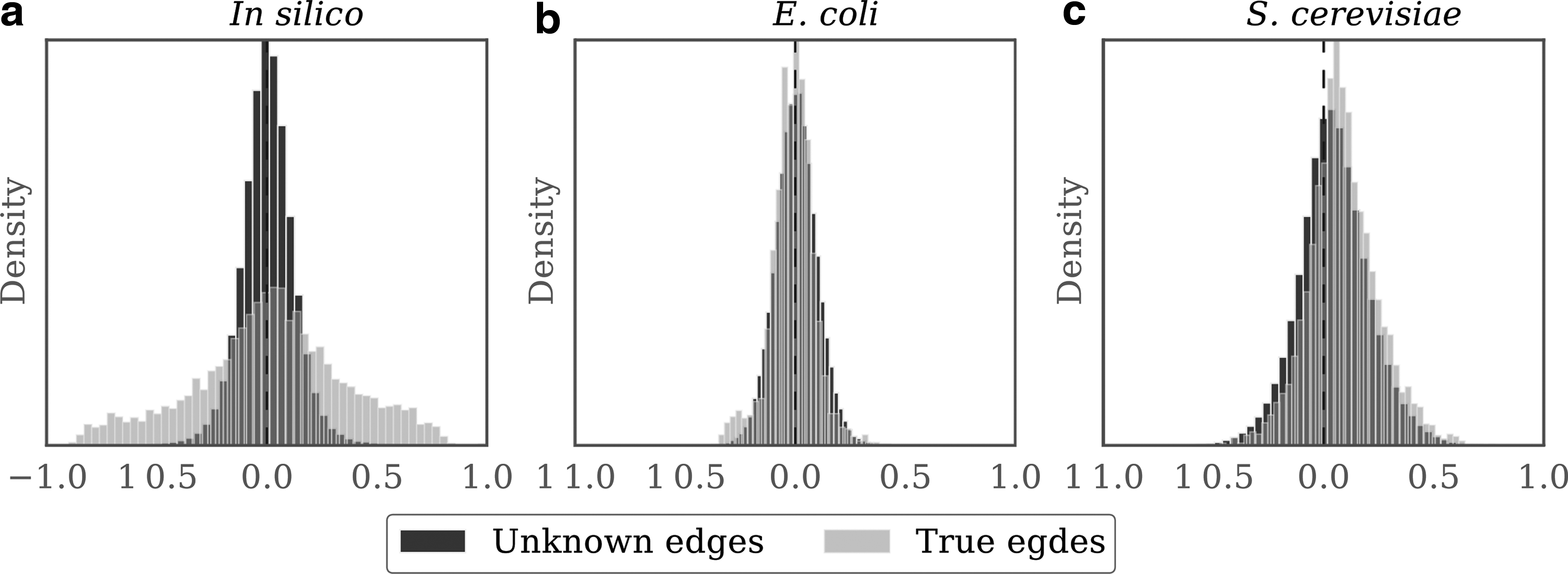
Here we investigate the signal present in each data set and show how it is related to the ability to reconstruct the GRN and to integrate PK. The core model used in CurInf and NoisInf assumes some degree of correlation between the mRNA levels of a TF and a gene for an interaction to be predicted. For time-series expression data, the model uses time-lagged relations, meaning that the mRNA level of a gene at time t should be related to the mRNA level of the TF at time \documentclass{aastex}\usepackage{amsbsy}\usepackage{amsfonts}\usepackage{amssymb}\usepackage{bm}\usepackage{mathrsfs}\usepackage{pifont}\usepackage{stmaryrd}\usepackage{textcomp}\usepackage{portland, xspace}\usepackage{amsmath, amsxtra}\usepackage{upgreek}\pagestyle{empty}\DeclareMathSizes{10}{9}{7}{6}\begin{document} $$t - 1$$ \end{document} . For steady state experiments, the system is assumed to reach equilibrium and thus the TF–target relation is considered without time lag. We calculated the TF–target correlations for the gold standard interactions of each data set as well as the correlation of the unknown interactions. The resulting histograms are shown in Figure 4. For the in silico data, the distribution of the gold standard edges shows a clear distinction from the unknown edges with more values greater than \documentclass{aastex}\usepackage{amsbsy}\usepackage{amsfonts}\usepackage{amssymb}\usepackage{bm}\usepackage{mathrsfs}\usepackage{pifont}\usepackage{stmaryrd}\usepackage{textcomp}\usepackage{portland, xspace}\usepackage{amsmath, amsxtra}\usepackage{upgreek}\pagestyle{empty}\DeclareMathSizes{10}{9}{7}{6}\begin{document} $$0.5$$ \end{document} and less than \documentclass{aastex}\usepackage{amsbsy}\usepackage{amsfonts}\usepackage{amssymb}\usepackage{bm}\usepackage{mathrsfs}\usepackage{pifont}\usepackage{stmaryrd}\usepackage{textcomp}\usepackage{portland, xspace}\usepackage{amsmath, amsxtra}\usepackage{upgreek}\pagestyle{empty}\DeclareMathSizes{10}{9}{7}{6}\begin{document} $$- 0.5$$ \end{document} , making it easier for most inference algorithms to predict. For the real data sets from E. coli and S. cerevisiae, the gene expression data do not show clear support for all the gold standard, which made those two data sets difficult for the 35 inference methods evaluated with this benchmark (Marbach et al., 2012). As shown in Figure 2, CurInf was able to integrate curated PK more than NoisInf in those two data sets that do not have strong support for the gold standard GRN.

FIG. 4.

Signal in each gene expression data set. For each data set, we plot two distributions to compare: (i) unknown edges: the correlation between the expression level of all genes and TFs and (ii) true edges: the correlation between TF–target pairs present in the gold standard GRN. The two distributions in the in silico data have a clear distinction with more correlations more than \documentclass{aastex}\usepackage{amsbsy}\usepackage{amsfonts}\usepackage{amssymb}\usepackage{bm}\usepackage{mathrsfs}\usepackage{pifont}\usepackage{stmaryrd}\usepackage{textcomp}\usepackage{portland, xspace}\usepackage{amsmath, amsxtra}\usepackage{upgreek}\pagestyle{empty}\DeclareMathSizes{10}{9}{7}{6}\begin{document} $$0.5$$ \end{document} and less than \documentclass{aastex}\usepackage{amsbsy}\usepackage{amsfonts}\usepackage{amssymb}\usepackage{bm}\usepackage{mathrsfs}\usepackage{pifont}\usepackage{stmaryrd}\usepackage{textcomp}\usepackage{portland, xspace}\usepackage{amsmath, amsxtra}\usepackage{upgreek}\pagestyle{empty}\DeclareMathSizes{10}{9}{7}{6}\begin{document} $$- 0.5$$ \end{document} for the gold standard. For the real data sets from Escherichia coli and Saccharomyces cerevisiae, the gene expression data do not show clear support for all the gold standard, which made those two data sets difficult to predict their GRN. CurInf was able to achieve higher accuracy in those real data sets than NoisInf.

3.5. Effect of prior weight parameter

We investigated the effect of the prior weight parameter on the accuracy of the predicted GRN. Different values of the weight parameter \documentclass{aastex}\usepackage{amsbsy}\usepackage{amsfonts}\usepackage{amssymb}\usepackage{bm}\usepackage{mathrsfs}\usepackage{pifont}\usepackage{stmaryrd}\usepackage{textcomp}\usepackage{portland, xspace}\usepackage{amsmath, amsxtra}\usepackage{upgreek}\pagestyle{empty}\DeclareMathSizes{10}{9}{7}{6}\begin{document} $${ \theta _i}$$ \end{document} [in Equations (9) and (10)] were tested in both NoisInf and CurInf (Supplementary Fig. S2). For simplicity, we use the same value of \documentclass{aastex}\usepackage{amsbsy}\usepackage{amsfonts}\usepackage{amssymb}\usepackage{bm}\usepackage{mathrsfs}\usepackage{pifont}\usepackage{stmaryrd}\usepackage{textcomp}\usepackage{portland, xspace}\usepackage{amsmath, amsxtra}\usepackage{upgreek}\pagestyle{empty}\DeclareMathSizes{10}{9}{7}{6}\begin{document} $${ \theta _i}$$ \end{document} for all genes in each experiment. All the gold standard was used as PK. A prior weight of 1 means no weight is given to the PK, whereas smaller values increase the PK effect. We found that a prior weight of \documentclass{aastex}\usepackage{amsbsy}\usepackage{amsfonts}\usepackage{amssymb}\usepackage{bm}\usepackage{mathrsfs}\usepackage{pifont}\usepackage{stmaryrd}\usepackage{textcomp}\usepackage{portland, xspace}\usepackage{amsmath, amsxtra}\usepackage{upgreek}\pagestyle{empty}\DeclareMathSizes{10}{9}{7}{6}\begin{document} $$0.01$$ \end{document} or less was enough to produce the best accuracy in our test data. A similar effect was found in Greenfield et al. (2013) when testing the MEN method, where they had a slight peak at a prior weight of \documentclass{aastex}\usepackage{amsbsy}\usepackage{amsfonts}\usepackage{amssymb}\usepackage{bm}\usepackage{mathrsfs}\usepackage{pifont}\usepackage{stmaryrd}\usepackage{textcomp}\usepackage{portland, xspace}\usepackage{amsmath, amsxtra}\usepackage{upgreek}\pagestyle{empty}\DeclareMathSizes{10}{9}{7}{6}\begin{document} $$0.01$$ \end{document} .

3.6. Using bounded CV

We tested our proposed heuristic to provide a bounded search space for the weight of the penalty term. Both CurInf and NoisInf use CV to find the penalty term weight parameter \documentclass{aastex}\usepackage{amsbsy}\usepackage{amsfonts}\usepackage{amssymb}\usepackage{bm}\usepackage{mathrsfs}\usepackage{pifont}\usepackage{stmaryrd}\usepackage{textcomp}\usepackage{portland, xspace}\usepackage{amsmath, amsxtra}\usepackage{upgreek}\pagestyle{empty}\DeclareMathSizes{10}{9}{7}{6}\begin{document} $$\alpha$$ \end{document} in the elastic net, Equations (9) and (10), when incorporating PK. Supplementary Figure S3 shows the accuracy using bounded CV versus unrestricted CV for both CurInf and NoisInf. Applying bounded CV improved the accuracy for CurInf when the PK is not well supported by the gene expression data as in the E. coli and S. cerevisiae data sets.

4. Discussion and Conclusion

In this work, we developed PEAK, a system to integrate both noisy and curated structure PK in the same GRN inference model based on the Inferelator algorithm (Bonneau et al., 2006). Curated or reliable PK comes from experimentally verified pathways, whereas noisy PK can be any supporting information about the network structure that does not necessarily imply regulatory relations, such as PPIs. To our knowledge, the integration of curated PK has not been addressed by any previous method, especially when the PK is not well supported by the gene expression data. We have shown that such poor PK support exists in real data than in synthetic data. We present a novel method in GRN inference, CurInf, to integrate curated PK from experimentally validated TF–target interactions. For noisy PK, we use a similar approach to the robust method MEN (Greenfield et al., 2013), which we call NoisInf. Both CurInf and NoisInf add PK to the model but in different ways that account for the confidence given to the PK.

Our testing on synthetic data as well as real data from E. coli and S. cerevisiae shows that adding PK significantly improved the accuracy of the predicted GRN. Moreover, CurInf is superior to NoisInf in the integration of curated PK, even if the PK is not well supported by the gene expression data. The improvement is more pronounced in the E. coli and S. cerevisiae data than in the synthetic data, because our method is designed to address gene expression data that may poorly support the PK. The difference in accuracy between synthetic and real data can be because of the expected complexity of the latter, and that the synthetic expression data were generated with a known network while the regulatory networks of E. coli and S. cerevisiae are still not complete. It is possible that true TF–target interactions exist among the predicted interactions that are considered false positives, which reduces the AUPR score.

Adding PK enabled PEAK to discover new validated interactions that are not in the gold standard. As the gold standard for the E. coli benchmark was created in 2010 from RegulonDB version 7, new interactions have been added to the database. We validated CurInf predictions that are considered false positives according to the gold standard using the most recent RegulonDB version 9. We were able to validate 128 of the computationally inferred interactions, including 17 with strong experimental evidence. For example, in the E. coli-predicted GRN using \documentclass{aastex}\usepackage{amsbsy}\usepackage{amsfonts}\usepackage{amssymb}\usepackage{bm}\usepackage{mathrsfs}\usepackage{pifont}\usepackage{stmaryrd}\usepackage{textcomp}\usepackage{portland, xspace}\usepackage{amsmath, amsxtra}\usepackage{upgreek}\pagestyle{empty}\DeclareMathSizes{10}{9}{7}{6}\begin{document} $$100 \%$$ \end{document} of the gold standard as PK, CurInf predicted Lrp as a TF for cadA, which is not in the gold standard. We validated this regulatory relation, and it was recently published that Lrp is a regulator of cadA (Ruiz et al., 2011). Similarly, CurInf predicted MarA to be a TF for ybjC, which was validated by Martin and Rosner (2011).

Thus, better integration of PK improves the accuracy and enables the inference algorithm to predict new potential regulatory relations. High-ranked predicted interactions, especially with a consensus of multiple computational methods, can be potential subjects for biologists to test and validate experimentally.

Footnotes

Acknowledgments

We thank Dr. Bert Huang for his useful discussions and Dr. Richard Bonneau for providing us with the source code of Mixed CLR and the Inferelator.

Author Disclosure Statement

No competing financial interests exist.

References

Barrett

, Wilhite

S.E.

, Ledoux

, et al. 2013. NCBI GEO: Archive for functional genomics data sets-update. Nucleic Acids Res. 41(D1), D991–D995.

Bolstad

B.M.

, Irizarry

R.A.

, Åstrand

, et al. 2003. A comparison of normalization methods for high density oligonucleotide array data based on variance and bias. Bioinformatics, 19, 185–193.

Bonneau

, Reiss

D.J.

, Shannon

, et al. 2006. The Inferelator: An algorithm for learning parsimonious regulatory networks from systems-biology data sets de novo. Genome Biol. 7, R36.

Chen

, Cairelli

M.J.

, Kilicoglu

, et al. 2014. Augmenting microarray data with literature-based knowledge to enhance gene regulatory network inference. PLoS Comput. Biol. 10, e1003666.

De Smet

, and Marchal

. 2010. Advantages and limitations of current network inference methods. Nat. Rev. Microbiol. 8, 717–729.

Friedman

, Hastie

, and Tibshirani

2010. Regularization paths for generalized linear models via coordinate descent. J. Stat.Softw., 33, 1.

Gama-Castro

, Salgado

, Santos-Zavaleta

, et al. 2016. RegulonDB version 9.0: High-level integration of gene regulation, coexpression, motif clustering and beyond. Nucl. Acids Res. 44(D1), D133–D143.

Greenfield

, Madar

, Ostrer

, et al. 2010. DREAM4: Combining genetic and dynamic information to identify biological networks and dynamical models. PLoS One, 5, e13397.

Greenfield

, Hafemeister

, and Bonneau

2013. Robust data-driven incorporation of prior knowledge into the inference of dynamic regulatory networks. Bioinformatics, 29, 1060–1067.

10.

Haury

A.-C.

, Mordelet

, Vera-Licona

, et al. 2012. TIGRESS: Trustful inference of gene regulation using stability selection. BMC Syst. Biol. 6, 145.

11.

Hickman

G.J.

, and Hodgman

T.C.

2009. Inference of gene regulatory networks using boolean-network inference methods. J. Bioinform. Comput. Biol. 7, 1013–1029.

12.

Isci

, Dogan

, Ozturk

, et al. 2014. Bayesian network prior: Network analysis of biological data using external knowledge. Bioinformatics, 30, 860–867.

13.

Liu

Z.-P.

2015. Reverse engineering of genome-wide gene regulatory networks from gene expression data. Curr. Genomics, 16, 3–22.

14.

, Raftery

A.E.

, Dombek

K.M.

, et al. 2012. Integrating external biological knowledge in the construction of regulatory networks from time-series expression data. BMC Syst. Biol. 6, 101.

15.

Madar

, Greenfield

, Vanden-Eijnden

, et al. 2010. DREAM3: Network inference using dynamic context likelihood of relatedness and the Inferelator. PLoS One, 5, e9803.

16.

Marbach

, Costello

J.C.

, Kueffner

, et al. 2012. Wisdom of crowds for robust gene network inference. Nat. Methods, 9, 796–804.

17.

Martin

R.G.

, and Rosner

J.L.

2011. Promoter discrimination at class I MarA regulon promoters mediated by glutamic acid 89 of the MarA transcriptional activator of Escherichia coli. J. Bacteriol., 193, 506–515.

18.

Omony

2014. Biological network inference: A review of methods and assessment of tools and techniques. Annu. Res. Rev. Biol. 4, 577–601.

19.

Penfold

C.A.

, and Wild

D.L.

2011. How to infer gene networks from expression profiles, revisited. Interface Focus, 1, 857–870.

20.

Ruiz

, Haneburger

, and Jung

2011. Identification of ArgP and Lrp as transcriptional regulators of lysP, the gene encoding the specific lysine permease of Escherichia coli. J. Bacteriol. 193, 2536–2548.

21.

Studham

M.E.

, Tjärnberg

, Nordling

T.E.

, et al. 2014. Functional association networks as priors for gene regulatory network inference. Bioinformatics, 30, i130–i138.

22.

Tan

, Alshalalfa

, Alhajj

, et al. 2011. Influence of prior knowledge in constraint-based learning of gene regulatory networks. IEEE/ACM Trans. Comput. Biol. Bioinform. 8, 130–142.

23.

Wang

Y.R.

, and Huang

2014. Review on statistical methods for gene network reconstruction using expression data. J. Theor. Biol. 362, 53–61.

24.

Werhli

A.V.

, and Husmeier

2007. Reconstructing gene regulatory networks with Bayesian networks by combining expression data with multiple sources of prior knowledge. Stat. Appl. Genet. Mol.Biol. 6.

25.

Zou

, and Hastie

2005. Regularization and variable selection via the Elastic net. J. R. Stat. Soc. B, 67, 301–320.

26.

Zou

, and Zhang

H.H.

2009. On the adaptive elastic-net with a diverging number of parameters. Ann. Stat. 37, 1733.

27.

Zou

, and Conzen

S.D.

2005. A new dynamic Bayesian network (DBN) approach for identifying gene regulatory networks from time course microarray data. Bioinformatics, 21, 71–79.

Supplementary Material

Please find the following supplemental material available below.

For Open Access articles published under a Creative Commons License, all supplemental material carries the same license as the article it is associated with.

For non-Open Access articles published, all supplemental material carries a non-exclusive license, and permission requests for re-use of supplemental material or any part of supplemental material shall be sent directly to the copyright owner as specified in the copyright notice associated with the article.

0.00 MB

0.07 MB