Disease-causing pathogens such as viruses introduce their proteins into the host cells in which they interact with the host's proteins, enabling the virus to replicate inside the host. These interactions between pathogen and host proteins are key to understanding infectious diseases. Often multiple diseases involve phylogenetically related or biologically similar pathogens. Here we present a multitask learning method to jointly model interactions between human proteins and three different but related viruses: Hepatitis C, Ebola virus, and Influenza A. Our multitask matrix completion-based model uses a shared low-rank structure in addition to a task-specific sparse structure to incorporate the various interactions. We obtain between 7 and 39 percentage points improvement in predictive performance over prior state-of-the-art models. We show how our model's parameters can be interpreted to reveal both general and specific interaction-relevant characteristics of the viruses. Our code is available online.*
1. Introduction
Infectious diseases such as H1N1 influenza, the recent Ebola outbreak, and bacterial infections such as the recurrent Salmonella and Escherichia coli outbreaks are a major health concern worldwide, causing millions of illnesses and many deaths each year. Key to the infection process are host–pathogen interactions at the molecular level, in which pathogen proteins physically bind to human proteins to manipulate important biological processes in the host cell, to evade the host's immune response, and to multiply within the host. Very little is known about these protein–protein interactions (PPIs) between pathogen and host proteins for any individual disease. However, such PPI data are widely available across several diseases, and the central question in this article is: Can we model host–pathogen PPIs better by leveraging data across multiple diseases? This is of particular interest for lesser known or recently evolved diseases, in which the data are particularly scarce. Furthermore, it allows us to learn models that generalize better across diseases by modeling global phenomena related to infection.
An elegant way to formulate the interaction prediction problem is through a graph completion-based framework, in which we have several bipartite graphs over multiple hosts and pathogens. Nodes in the graphs represent host proteins (circles) and pathogen proteins (triangles), with edges between them representing interactions (host protein \documentclass{aastex}\usepackage{amsbsy}\usepackage{amsfonts}\usepackage{amssymb}\usepackage{bm}\usepackage{mathrsfs}\usepackage{pifont}\usepackage{stmaryrd}\usepackage{textcomp}\usepackage{portland, xspace}\usepackage{amsmath, amsxtra}\usepackage{upgreek}\pagestyle{empty}\DeclareMathSizes{10}{9}{7}{6}\begin{document}
$$ \frac { { interacts } } { } $$
\end{document} pathogen protein). Given some observed edges (interactions obtained from laboratory-based experiments), we wish to predict the other edges in the graphs. Such bipartite graphs arise in a plethora of problems, including recommendation systems (user \documentclass{aastex}\usepackage{amsbsy}\usepackage{amsfonts}\usepackage{amssymb}\usepackage{bm}\usepackage{mathrsfs}\usepackage{pifont}\usepackage{stmaryrd}\usepackage{textcomp}\usepackage{portland, xspace}\usepackage{amsmath, amsxtra}\usepackage{upgreek}\pagestyle{empty}\DeclareMathSizes{10}{9}{7}{6}\begin{document}
$$ \frac { { prefers } } { } $$
\end{document} movie), citation networks (author \documentclass{aastex}\usepackage{amsbsy}\usepackage{amsfonts}\usepackage{amssymb}\usepackage{bm}\usepackage{mathrsfs}\usepackage{pifont}\usepackage{stmaryrd}\usepackage{textcomp}\usepackage{portland, xspace}\usepackage{amsmath, amsxtra}\usepackage{upgreek}\pagestyle{empty}\DeclareMathSizes{10}{9}{7}{6}\begin{document}
$$ \frac { { cites } } { } $$
\end{document} article), and disease–gene networks (gene \documentclass{aastex}\usepackage{amsbsy}\usepackage{amsfonts}\usepackage{amssymb}\usepackage{bm}\usepackage{mathrsfs}\usepackage{pifont}\usepackage{stmaryrd}\usepackage{textcomp}\usepackage{portland, xspace}\usepackage{amsmath, amsxtra}\usepackage{upgreek}\pagestyle{empty}\DeclareMathSizes{10}{9}{7}{6}\begin{document}
$$ \frac { { influences } } { } $$
\end{document} disease). In our problem, each bipartite graph \documentclass{aastex}\usepackage{amsbsy}\usepackage{amsfonts}\usepackage{amssymb}\usepackage{bm}\usepackage{mathrsfs}\usepackage{pifont}\usepackage{stmaryrd}\usepackage{textcomp}\usepackage{portland, xspace}\usepackage{amsmath, amsxtra}\usepackage{upgreek}\pagestyle{empty}\DeclareMathSizes{10}{9}{7}{6}\begin{document}
$${ \cal G}$$
\end{document} can be represented using a matrix M, in which the rows correspond to pathogen proteins and columns correspond to host proteins. The matrix entry \documentclass{aastex}\usepackage{amsbsy}\usepackage{amsfonts}\usepackage{amssymb}\usepackage{bm}\usepackage{mathrsfs}\usepackage{pifont}\usepackage{stmaryrd}\usepackage{textcomp}\usepackage{portland, xspace}\usepackage{amsmath, amsxtra}\usepackage{upgreek}\pagestyle{empty}\DeclareMathSizes{10}{9}{7}{6}\begin{document}
$${M_{ij}}$$
\end{document} encodes the edge between pathogen protein i and host protein j from the graph, with \documentclass{aastex}\usepackage{amsbsy}\usepackage{amsfonts}\usepackage{amssymb}\usepackage{bm}\usepackage{mathrsfs}\usepackage{pifont}\usepackage{stmaryrd}\usepackage{textcomp}\usepackage{portland, xspace}\usepackage{amsmath, amsxtra}\usepackage{upgreek}\pagestyle{empty}\DeclareMathSizes{10}{9}{7}{6}\begin{document}
$${M_{ij}} = 1$$
\end{document} for the observed interactions. Thus, the graph completion problem can be mathematically modeled as a matrix completion problem (Candes and Recht, 2009).
Most of the prior work on host–pathogen PPI prediction has modeled each bipartite graph separately, and hence cannot exploit the similarities in the edges across the various graphs. Here we present a multitask matrix completion method that jointly models several bipartite graphs by sharing information across them. From the multitask perspective, a task is the graph between one host and one pathogen (can also be seen as interactions relevant to one disease). We focus on the setting in which we have a single host species (human) and several related viruses, in which we hope to gain from the fact that similar viruses will have similar strategies to infect and hijack biological processes in the human body. Such opportunities for sharing arise in other applications as well: for instance, predicting user preferences in movies may inform preferences in selection of books, or vice versa, as movies and books are semantically related. Multitask learning-based models that incorporate and exploit these correlations should benefit from the additional information.
Our multitask matrix completion-based model is motivated by the following biological intuition governing protein interactions across diseases.
1. An interaction depends on the structural properties of the proteins, which are conserved across similar viruses as they have evolved from common ancestors. Our model thus needs a component to capture these latent similarities, which is shared across tasks.
2. In addition to the shared properties already discussed, each pathogen has also evolved specialized mechanisms to target host proteins. These are unique to the pathogen and can be expressed using a task-specific parameter in the model.
This leads us to the following model that incorporates the mentioned ideas. The interactions matrix Mt of task t can be written as \documentclass{aastex}\usepackage{amsbsy}\usepackage{amsfonts}\usepackage{amssymb}\usepackage{bm}\usepackage{mathrsfs}\usepackage{pifont}\usepackage{stmaryrd}\usepackage{textcomp}\usepackage{portland, xspace}\usepackage{amsmath, amsxtra}\usepackage{upgreek}\pagestyle{empty}\DeclareMathSizes{10}{9}{7}{6}\begin{document}
$${M_t} = { \mu _t}*$$
\end{document} (shared component)\documentclass{aastex}\usepackage{amsbsy}\usepackage{amsfonts}\usepackage{amssymb}\usepackage{bm}\usepackage{mathrsfs}\usepackage{pifont}\usepackage{stmaryrd}\usepackage{textcomp}\usepackage{portland, xspace}\usepackage{amsmath, amsxtra}\usepackage{upgreek}\pagestyle{empty}\DeclareMathSizes{10}{9}{7}{6}\begin{document}
$$+ ( 1 - { \mu _t} ) *$$
\end{document} (specific component) with hyperparameter \documentclass{aastex}\usepackage{amsbsy}\usepackage{amsfonts}\usepackage{amssymb}\usepackage{bm}\usepackage{mathrsfs}\usepackage{pifont}\usepackage{stmaryrd}\usepackage{textcomp}\usepackage{portland, xspace}\usepackage{amsmath, amsxtra}\usepackage{upgreek}\pagestyle{empty}\DeclareMathSizes{10}{9}{7}{6}\begin{document}
$${ \mu _t}$$
\end{document}, allowing each task to customize its amount of shared and specific components.
To incorporate the mentioned ideas, we assume that the interactions matrix M is generated from two components. The first component has low-rank latent factors over the human and virus proteins, with these latent factors jointly learned over all tasks. The second component involves a task-specific parameter, on which we additionally impose a sparsity constraint as we do not want this parameter to overfit the data. Section 3 discusses our model in detail. We trade-off the relative importance of the two components using task-specific hyperparameters. Our model can thus learn what is conserved and what is different across pathogens, rather than having to specify it manually.
The key challenges in inducing such a model are as follows. (1) In addition to the interactions from each graph, it should exploit information available in the form of features. (2) Exploiting features is particularly crucial because the graph \documentclass{aastex}\usepackage{amsbsy}\usepackage{amsfonts}\usepackage{amssymb}\usepackage{bm}\usepackage{mathrsfs}\usepackage{pifont}\usepackage{stmaryrd}\usepackage{textcomp}\usepackage{portland, xspace}\usepackage{amsmath, amsxtra}\usepackage{upgreek}\pagestyle{empty}\DeclareMathSizes{10}{9}{7}{6}\begin{document}
$${ \cal G}$$
\end{document} is often extremely sparse, that is, there are a large number of nodes and very few edges are observed. There will be proteins (i.e., nodes) that are not involved in any known interactions—called the cold start problem in the recommendation systems community. The model should be able to predict the existence of links (or their absence) between such prior “unseen” node pairs. This is of particular significance in graphs that capture biological phenomena. For instance, the host–pathogen PPI network of human Ebola virus (column 3, Table 2) has \documentclass{aastex}\usepackage{amsbsy}\usepackage{amsfonts}\usepackage{amssymb}\usepackage{bm}\usepackage{mathrsfs}\usepackage{pifont}\usepackage{stmaryrd}\usepackage{textcomp}\usepackage{portland, xspace}\usepackage{amsmath, amsxtra}\usepackage{upgreek}\pagestyle{empty}\DeclareMathSizes{10}{9}{7}{6}\begin{document}
$$\approx$$
\end{document}90 observed edges (equivalent to 0.06% of the possible edges), which involve only 2 distinct virus proteins. (3) A side effect of having scarce data is the availability of a large number of unlabeled examples, that is, pairs of nodes with no edge between them. These unlabeled examples can contain information about the graph as a whole, and a good model should be able to use them.
The main contributions of this work are as follows.
• We extend a prior matrix completion model (Abernethy et al., 2009) to the multitask setting. This extension is new.
• Unlike most prior approaches, our model exploits node-based features, which allows us to deal with the “cold start” problem (generating predictions on unseen nodes).
• We apply the model to an important, real-world problem—prediction of interactions in disease-relevant host–pathogen protein networks, for multiple related diseases. We demonstrate the superior performance of our model over prior state-of-the-art multitask models.
• We use unlabeled data to initialize the parameters of our model, which serves as a prior. This gives us a modest boost in prediction performance.
1.1. Background: Host–pathogen PPIs
The experimental discovery of host–pathogen protein–protein interactions (HP PPIs) involves biochemical and biophysical methods such as coimmunoprecipitation, yeast two-hybrid assays, and cocrystalization. The HP PPIs from several small-scale and high-throughput experiments are aggregated by databases such as MINT (Chatraryamontri et al., 2009), HPIDB (Kumar and Nanduri, 2010), and PHISTO (Tekir et al., 2012) by literature curation. These databases are valuable sources of information to bioinformaticians for developing models.
1.1.1. Prediction of host–pathogen PPIs
The most reliable experimental methods for studying PPIs are often very time consuming and expensive, making it hard to investigate the prohibitively large set of possible host–pathogen interactions—for example, the bacterium Bacillus anthracis that causes anthrax has about 2321 proteins, which when coupled with the 100,000 or so human proteins gives \documentclass{aastex}\usepackage{amsbsy}\usepackage{amsfonts}\usepackage{amssymb}\usepackage{bm}\usepackage{mathrsfs}\usepackage{pifont}\usepackage{stmaryrd}\usepackage{textcomp}\usepackage{portland, xspace}\usepackage{amsmath, amsxtra}\usepackage{upgreek}\pagestyle{empty}\DeclareMathSizes{10}{9}{7}{6}\begin{document}
$$\approx$$
\end{document}232 million protein pairs to test experimentally. Computational techniques complement laboratory-based methods by predicting highly probable PPIs. These techniques use the known interactions data from previous experiments and predict the most plausible new interactions. In particular, supervised machine learning-based methods use the few known interactions as training data and formulate the interaction prediction problem in a classification setting, with target classes “interacting” or “noninteracting.” Features are derived using various attributes of the two proteins such as protein sequences from UniProt (UniProt Consortium, 2011), protein structure from PDB, and gene ontology (GO) from GO database (Ashburner et al., 2000).
1.2. Prior work
Most of the prior work in PPI prediction has focused on building models separately for individual organisms (Chen and Liu, 2005; Qi et al., 2006; Singh et al., 2006; Wu et al., 2006) or on building a model specific to a disease in the case of HP PPI prediction (Dyer et al., 2007; Qi et al., 2009; Tastan et al., 2009; Kshirsagar et al., 2012). There has been little work on combining PPI data sets with the goal of improving prediction performance for multiple organisms. Qi et al. (2010) proposed a semisupervised multitask framework to predict PPIs from partially labeled reference sets. Kshirsagar et al. (2013) developed a task regularization-based framework called multitask pathway-based learning (MTPL) that incorporates the similarity in biological pathways targeted by various diseases to couple multiple tasks together. Matrix factorization-based PPI prediction has seen very little work, mainly because of the extremely sparse nature of these data sets that makes it very difficult to get reliable predictors. Xu et al. (2010) used a CMF-based approach in a multitask learning setting for within-species PPI prediction. The methods used in all prior work on PPI prediction do not explicitly model the features of the proteins and cannot be applied on proteins that have no known interactions available. Our work addresses both these issues.
A majority of the prior work in the relevant areas of collaborative filtering and link prediction includes single relation models that use neighborhood-based prediction (Sarwar et al., 2001), matrix factorization-based approaches (Koren et al., 2009; Menon and Elkan, 2011), and Bayesian approaches using graphical models (Jin et al., 2002; Phung et al., 2009). There have also been multitask approaches on link prediction (Singh and Gordon, 2008; Li et al., 2009; Cao et al., 2010; Zhang et al., 2012); however, many of those models do not incorporate features of the nodes in the graph. Menon and Elkan (2011) combine linear and bilinear features, latent parameters on the nodes, and several other parameters into a function that minimizes a ranking loss for link prediction in a single graph. Abernethy et al. (2009) cast the problem of matrix completion in terms of the abstract problem of learning linear operators. Their framework allows the incorporation of features and kernels. We extend their bilinear model for the multitask setting. There has been a lot of work on other low-rank models for multitask learning (Ando and Zhang, 2005; Ji and Ye, 2009; Chen et al., 2012, 2013). Another related line of work is coembedding, in which the goal is to embed different types of objects in the same shared lower dimensional space (Mirzazadeh et al., 2015).
2. Bilinear Low-Rank Matrix Decomposition
In this section, we present the matrix decomposition model that we extend for the multitask scenario. In the context of our problem, at a high level, this model states that protein interactions can be expressed as dot products of features in a lower dimensional subspace.
Let \documentclass{aastex}\usepackage{amsbsy}\usepackage{amsfonts}\usepackage{amssymb}\usepackage{bm}\usepackage{mathrsfs}\usepackage{pifont}\usepackage{stmaryrd}\usepackage{textcomp}\usepackage{portland, xspace}\usepackage{amsmath, amsxtra}\usepackage{upgreek}\pagestyle{empty}\DeclareMathSizes{10}{9}{7}{6}\begin{document}
$${{ \cal G}_t}$$
\end{document} be a bipartite graph connecting nodes of type \documentclass{aastex}\usepackage{amsbsy}\usepackage{amsfonts}\usepackage{amssymb}\usepackage{bm}\usepackage{mathrsfs}\usepackage{pifont}\usepackage{stmaryrd}\usepackage{textcomp}\usepackage{portland, xspace}\usepackage{amsmath, amsxtra}\usepackage{upgreek}\pagestyle{empty}\DeclareMathSizes{10}{9}{7}{6}\begin{document}
$$\upsilon$$
\end{document} with nodes of type \documentclass{aastex}\usepackage{amsbsy}\usepackage{amsfonts}\usepackage{amssymb}\usepackage{bm}\usepackage{mathrsfs}\usepackage{pifont}\usepackage{stmaryrd}\usepackage{textcomp}\usepackage{portland, xspace}\usepackage{amsmath, amsxtra}\usepackage{upgreek}\pagestyle{empty}\DeclareMathSizes{10}{9}{7}{6}\begin{document}
$$\varsigma$$
\end{document}. Let there be mt nodes of type \documentclass{aastex}\usepackage{amsbsy}\usepackage{amsfonts}\usepackage{amssymb}\usepackage{bm}\usepackage{mathrsfs}\usepackage{pifont}\usepackage{stmaryrd}\usepackage{textcomp}\usepackage{portland, xspace}\usepackage{amsmath, amsxtra}\usepackage{upgreek}\pagestyle{empty}\DeclareMathSizes{10}{9}{7}{6}\begin{document}
$$\upsilon$$
\end{document} and nt nodes of type \documentclass{aastex}\usepackage{amsbsy}\usepackage{amsfonts}\usepackage{amssymb}\usepackage{bm}\usepackage{mathrsfs}\usepackage{pifont}\usepackage{stmaryrd}\usepackage{textcomp}\usepackage{portland, xspace}\usepackage{amsmath, amsxtra}\usepackage{upgreek}\pagestyle{empty}\DeclareMathSizes{10}{9}{7}{6}\begin{document}
$$\varsigma$$
\end{document}. We denote by \documentclass{aastex}\usepackage{amsbsy}\usepackage{amsfonts}\usepackage{amssymb}\usepackage{bm}\usepackage{mathrsfs}\usepackage{pifont}\usepackage{stmaryrd}\usepackage{textcomp}\usepackage{portland, xspace}\usepackage{amsmath, amsxtra}\usepackage{upgreek}\pagestyle{empty}\DeclareMathSizes{10}{9}{7}{6}\begin{document}
$$M \in { \mathbb{R}^{{m_t} \times {n_t}}}$$
\end{document} the matrix representing the edges in \documentclass{aastex}\usepackage{amsbsy}\usepackage{amsfonts}\usepackage{amssymb}\usepackage{bm}\usepackage{mathrsfs}\usepackage{pifont}\usepackage{stmaryrd}\usepackage{textcomp}\usepackage{portland, xspace}\usepackage{amsmath, amsxtra}\usepackage{upgreek}\pagestyle{empty}\DeclareMathSizes{10}{9}{7}{6}\begin{document}
$${{ \cal G}_t}$$
\end{document}. Let the set of observed edges be \documentclass{aastex}\usepackage{amsbsy}\usepackage{amsfonts}\usepackage{amssymb}\usepackage{bm}\usepackage{mathrsfs}\usepackage{pifont}\usepackage{stmaryrd}\usepackage{textcomp}\usepackage{portland, xspace}\usepackage{amsmath, amsxtra}\usepackage{upgreek}\pagestyle{empty}\DeclareMathSizes{10}{9}{7}{6}\begin{document}
$$\Omega$$
\end{document}. Let \documentclass{aastex}\usepackage{amsbsy}\usepackage{amsfonts}\usepackage{amssymb}\usepackage{bm}\usepackage{mathrsfs}\usepackage{pifont}\usepackage{stmaryrd}\usepackage{textcomp}\usepackage{portland, xspace}\usepackage{amsmath, amsxtra}\usepackage{upgreek}\pagestyle{empty}\DeclareMathSizes{10}{9}{7}{6}\begin{document}
$${ \cal X}$$
\end{document} and \documentclass{aastex}\usepackage{amsbsy}\usepackage{amsfonts}\usepackage{amssymb}\usepackage{bm}\usepackage{mathrsfs}\usepackage{pifont}\usepackage{stmaryrd}\usepackage{textcomp}\usepackage{portland, xspace}\usepackage{amsmath, amsxtra}\usepackage{upgreek}\pagestyle{empty}\DeclareMathSizes{10}{9}{7}{6}\begin{document}
$${ \cal Y}$$
\end{document} be the feature spaces for the node types \documentclass{aastex}\usepackage{amsbsy}\usepackage{amsfonts}\usepackage{amssymb}\usepackage{bm}\usepackage{mathrsfs}\usepackage{pifont}\usepackage{stmaryrd}\usepackage{textcomp}\usepackage{portland, xspace}\usepackage{amsmath, amsxtra}\usepackage{upgreek}\pagestyle{empty}\DeclareMathSizes{10}{9}{7}{6}\begin{document}
$$\upsilon$$
\end{document} and \documentclass{aastex}\usepackage{amsbsy}\usepackage{amsfonts}\usepackage{amssymb}\usepackage{bm}\usepackage{mathrsfs}\usepackage{pifont}\usepackage{stmaryrd}\usepackage{textcomp}\usepackage{portland, xspace}\usepackage{amsmath, amsxtra}\usepackage{upgreek}\pagestyle{empty}\DeclareMathSizes{10}{9}{7}{6}\begin{document}
$$\varsigma$$
\end{document}, respectively. For the sake of notational convenience, we assume that the two feature spaces have the same dimension dt1. Let \documentclass{aastex}\usepackage{amsbsy}\usepackage{amsfonts}\usepackage{amssymb}\usepackage{bm}\usepackage{mathrsfs}\usepackage{pifont}\usepackage{stmaryrd}\usepackage{textcomp}\usepackage{portland, xspace}\usepackage{amsmath, amsxtra}\usepackage{upgreek}\pagestyle{empty}\DeclareMathSizes{10}{9}{7}{6}\begin{document}
$${{ \bf{x}}_i} \in { \cal X}$$
\end{document} denote the feature vector for a node i of type \documentclass{aastex}\usepackage{amsbsy}\usepackage{amsfonts}\usepackage{amssymb}\usepackage{bm}\usepackage{mathrsfs}\usepackage{pifont}\usepackage{stmaryrd}\usepackage{textcomp}\usepackage{portland, xspace}\usepackage{amsmath, amsxtra}\usepackage{upgreek}\pagestyle{empty}\DeclareMathSizes{10}{9}{7}{6}\begin{document}
$$\upsilon$$
\end{document} and \documentclass{aastex}\usepackage{amsbsy}\usepackage{amsfonts}\usepackage{amssymb}\usepackage{bm}\usepackage{mathrsfs}\usepackage{pifont}\usepackage{stmaryrd}\usepackage{textcomp}\usepackage{portland, xspace}\usepackage{amsmath, amsxtra}\usepackage{upgreek}\pagestyle{empty}\DeclareMathSizes{10}{9}{7}{6}\begin{document}
$${{ \bf{y}}_j} \in { \cal Y}$$
\end{document} be the feature vector for node j of type \documentclass{aastex}\usepackage{amsbsy}\usepackage{amsfonts}\usepackage{amssymb}\usepackage{bm}\usepackage{mathrsfs}\usepackage{pifont}\usepackage{stmaryrd}\usepackage{textcomp}\usepackage{portland, xspace}\usepackage{amsmath, amsxtra}\usepackage{upgreek}\pagestyle{empty}\DeclareMathSizes{10}{9}{7}{6}\begin{document}
$$\varsigma$$
\end{document}. The goal of the general matrix completion problem is to learn a function \documentclass{aastex}\usepackage{amsbsy}\usepackage{amsfonts}\usepackage{amssymb}\usepackage{bm}\usepackage{mathrsfs}\usepackage{pifont}\usepackage{stmaryrd}\usepackage{textcomp}\usepackage{portland, xspace}\usepackage{amsmath, amsxtra}\usepackage{upgreek}\pagestyle{empty}\DeclareMathSizes{10}{9}{7}{6}\begin{document}
$$f:{ \cal X} \times { \cal Y} \to \mathbb{R}$$
\end{document} that also explains the observed entries in the matrix M. We assume that the function f is bilinear on \documentclass{aastex}\usepackage{amsbsy}\usepackage{amsfonts}\usepackage{amssymb}\usepackage{bm}\usepackage{mathrsfs}\usepackage{pifont}\usepackage{stmaryrd}\usepackage{textcomp}\usepackage{portland, xspace}\usepackage{amsmath, amsxtra}\usepackage{upgreek}\pagestyle{empty}\DeclareMathSizes{10}{9}{7}{6}\begin{document}
$${ \cal X} \times { \cal Y}$$
\end{document}. This bilinear form was first introduced by Abernethy et al. (2009) and takes the following form:
\documentclass{aastex}\usepackage{amsbsy}\usepackage{amsfonts}\usepackage{amssymb}\usepackage{bm}\usepackage{mathrsfs}\usepackage{pifont}\usepackage{stmaryrd}\usepackage{textcomp}\usepackage{portland, xspace}\usepackage{amsmath, amsxtra}\usepackage{upgreek}\pagestyle{empty}\DeclareMathSizes{10}{9}{7}{6}\begin{document}
\begin{align*}
f ( {{ \rm{{ \bf x}}}_i} , {{ \rm{{ \bf y}}}_j} ) = { \rm{{ \bf x}}}_i^{ \rm T}H{{ \rm{{ \bf y}}}_j} = { \rm{{ \bf x}}}_i^{ \rm T}U{V^{ \rm T}}{{ \rm{{ \bf y}}}_j}. \tag{1}
\end{align*}
\end{document}
The factor \documentclass{aastex}\usepackage{amsbsy}\usepackage{amsfonts}\usepackage{amssymb}\usepackage{bm}\usepackage{mathrsfs}\usepackage{pifont}\usepackage{stmaryrd}\usepackage{textcomp}\usepackage{portland, xspace}\usepackage{amsmath, amsxtra}\usepackage{upgreek}\pagestyle{empty}\DeclareMathSizes{10}{9}{7}{6}\begin{document}
$$H \in { \mathbb{R}^{{d_t} \times {d_t}}}$$
\end{document} maps the two feature spaces \documentclass{aastex}\usepackage{amsbsy}\usepackage{amsfonts}\usepackage{amssymb}\usepackage{bm}\usepackage{mathrsfs}\usepackage{pifont}\usepackage{stmaryrd}\usepackage{textcomp}\usepackage{portland, xspace}\usepackage{amsmath, amsxtra}\usepackage{upgreek}\pagestyle{empty}\DeclareMathSizes{10}{9}{7}{6}\begin{document}
$${ \cal X}$$
\end{document} and \documentclass{aastex}\usepackage{amsbsy}\usepackage{amsfonts}\usepackage{amssymb}\usepackage{bm}\usepackage{mathrsfs}\usepackage{pifont}\usepackage{stmaryrd}\usepackage{textcomp}\usepackage{portland, xspace}\usepackage{amsmath, amsxtra}\usepackage{upgreek}\pagestyle{empty}\DeclareMathSizes{10}{9}{7}{6}\begin{document}
$${ \cal Y}$$
\end{document}. This model assumes that H has a low-rank factorization given by \documentclass{aastex}\usepackage{amsbsy}\usepackage{amsfonts}\usepackage{amssymb}\usepackage{bm}\usepackage{mathrsfs}\usepackage{pifont}\usepackage{stmaryrd}\usepackage{textcomp}\usepackage{portland, xspace}\usepackage{amsmath, amsxtra}\usepackage{upgreek}\pagestyle{empty}\DeclareMathSizes{10}{9}{7}{6}\begin{document}
$$H = UV^{ \rm T}$$
\end{document}, where \documentclass{aastex}\usepackage{amsbsy}\usepackage{amsfonts}\usepackage{amssymb}\usepackage{bm}\usepackage{mathrsfs}\usepackage{pifont}\usepackage{stmaryrd}\usepackage{textcomp}\usepackage{portland, xspace}\usepackage{amsmath, amsxtra}\usepackage{upgreek}\pagestyle{empty}\DeclareMathSizes{10}{9}{7}{6}\begin{document}
$$U \in { \mathbb{R}^{{d_t} \times k}}$$
\end{document} and \documentclass{aastex}\usepackage{amsbsy}\usepackage{amsfonts}\usepackage{amssymb}\usepackage{bm}\usepackage{mathrsfs}\usepackage{pifont}\usepackage{stmaryrd}\usepackage{textcomp}\usepackage{portland, xspace}\usepackage{amsmath, amsxtra}\usepackage{upgreek}\pagestyle{empty}\DeclareMathSizes{10}{9}{7}{6}\begin{document}
$$V \in { \mathbb{R}^{{d_t} \times k}}$$
\end{document}. The factors U and V project the two feature spaces to a common lower dimensional subspace of dimension k. Although the dimensionality of the feature spaces \documentclass{aastex}\usepackage{amsbsy}\usepackage{amsfonts}\usepackage{amssymb}\usepackage{bm}\usepackage{mathrsfs}\usepackage{pifont}\usepackage{stmaryrd}\usepackage{textcomp}\usepackage{portland, xspace}\usepackage{amsmath, amsxtra}\usepackage{upgreek}\pagestyle{empty}\DeclareMathSizes{10}{9}{7}{6}\begin{document}
$${ \cal X}$$
\end{document} and \documentclass{aastex}\usepackage{amsbsy}\usepackage{amsfonts}\usepackage{amssymb}\usepackage{bm}\usepackage{mathrsfs}\usepackage{pifont}\usepackage{stmaryrd}\usepackage{textcomp}\usepackage{portland, xspace}\usepackage{amsmath, amsxtra}\usepackage{upgreek}\pagestyle{empty}\DeclareMathSizes{10}{9}{7}{6}\begin{document}
$${ \cal Y}$$
\end{document} may be very large, the latent lower dimensional subspace is sufficient to capture all the information pertinent to interactions. To predict whether two new nodes (i.e., nodes with no observed edges) with features \documentclass{aastex}\usepackage{amsbsy}\usepackage{amsfonts}\usepackage{amssymb}\usepackage{bm}\usepackage{mathrsfs}\usepackage{pifont}\usepackage{stmaryrd}\usepackage{textcomp}\usepackage{portland, xspace}\usepackage{amsmath, amsxtra}\usepackage{upgreek}\pagestyle{empty}\DeclareMathSizes{10}{9}{7}{6}\begin{document}
$${{ \bf{p}}_i}$$
\end{document} and \documentclass{aastex}\usepackage{amsbsy}\usepackage{amsfonts}\usepackage{amssymb}\usepackage{bm}\usepackage{mathrsfs}\usepackage{pifont}\usepackage{stmaryrd}\usepackage{textcomp}\usepackage{portland, xspace}\usepackage{amsmath, amsxtra}\usepackage{upgreek}\pagestyle{empty}\DeclareMathSizes{10}{9}{7}{6}\begin{document}
$${{ \bf{q}}_j}$$
\end{document} interact, we simply need to compute the product: \documentclass{aastex}\usepackage{amsbsy}\usepackage{amsfonts}\usepackage{amssymb}\usepackage{bm}\usepackage{mathrsfs}\usepackage{pifont}\usepackage{stmaryrd}\usepackage{textcomp}\usepackage{portland, xspace}\usepackage{amsmath, amsxtra}\usepackage{upgreek}\pagestyle{empty}\DeclareMathSizes{10}{9}{7}{6}\begin{document}
$${ \bf p}_iUV^{ \rm T}{ \bf q}_j$$
\end{document}. This enables the model to avoid the cold start problem that many prior models suffer from. The objective function to learn the parameters of this model has two main terms: (1) a data-fitting term, which imposes a penalty for deviating from the observed entries in \documentclass{aastex}\usepackage{amsbsy}\usepackage{amsfonts}\usepackage{amssymb}\usepackage{bm}\usepackage{mathrsfs}\usepackage{pifont}\usepackage{stmaryrd}\usepackage{textcomp}\usepackage{portland, xspace}\usepackage{amsmath, amsxtra}\usepackage{upgreek}\pagestyle{empty}\DeclareMathSizes{10}{9}{7}{6}\begin{document}
$$\Omega$$
\end{document} and (2) a low-rank enforcing term on the matrix H.
The first term can be any loss function such as squared error, logistic loss, and hinge loss. We tried both squared error and logistic loss and found the performance to be similar. The squared error function has the advantage of being amenable to adaptive step-size-based optimization, which results in a much faster convergence. The low-rank constraint on H (mentioned in (2)) is NP-hard to solve and it is standard practice to replace it with either the trace norm or the nuclear norm. Minimizing the trace norm (i.e., sum of singular values) of \documentclass{aastex}\usepackage{amsbsy}\usepackage{amsfonts}\usepackage{amssymb}\usepackage{bm}\usepackage{mathrsfs}\usepackage{pifont}\usepackage{stmaryrd}\usepackage{textcomp}\usepackage{portland, xspace}\usepackage{amsmath, amsxtra}\usepackage{upgreek}\pagestyle{empty}\DeclareMathSizes{10}{9}{7}{6}\begin{document}
$$H = UV^{ \rm T}$$
\end{document} is equivalent to minimizing \documentclass{aastex}\usepackage{amsbsy}\usepackage{amsfonts}\usepackage{amssymb}\usepackage{bm}\usepackage{mathrsfs}\usepackage{pifont}\usepackage{stmaryrd}\usepackage{textcomp}\usepackage{portland, xspace}\usepackage{amsmath, amsxtra}\usepackage{upgreek}\pagestyle{empty}\DeclareMathSizes{10}{9}{7}{6}\begin{document}
$$\parallel U \parallel _F^2 + \parallel V \parallel _F^2$$
\end{document}. This choice makes the overall function easier to optimize:
\documentclass{aastex}\usepackage{amsbsy}\usepackage{amsfonts}\usepackage{amssymb}\usepackage{bm}\usepackage{mathrsfs}\usepackage{pifont}\usepackage{stmaryrd}\usepackage{textcomp}\usepackage{portland, xspace}\usepackage{amsmath, amsxtra}\usepackage{upgreek}\pagestyle{empty}\DeclareMathSizes{10}{9}{7}{6}\begin{document}
\begin{align*}
\begin{split} {\cal L} ( U , V ) & = \mathop \sum \limits_{ ( i ,
j ) \in \Omega } {{C_{ij}}} \ \ell ( {M_{ij}} , { \bf x}_i^{\rm
T}U{V^{\rm T}}{{ \bf y}_j} ) + \lambda ( \parallel U \parallel
_F^2 + \parallel V \parallel _F^2 ) \\ & { \rm{where}} \ \ell (
a , b ) = { ( a - b ) ^2}\end{split}.
\tag{2}
\end{align*}
\end{document}
The constant \documentclass{aastex}\usepackage{amsbsy}\usepackage{amsfonts}\usepackage{amssymb}\usepackage{bm}\usepackage{mathrsfs}\usepackage{pifont}\usepackage{stmaryrd}\usepackage{textcomp}\usepackage{portland, xspace}\usepackage{amsmath, amsxtra}\usepackage{upgreek}\pagestyle{empty}\DeclareMathSizes{10}{9}{7}{6}\begin{document}
$${c_{ij}}$$
\end{document} is the weight/cost associated with the edge \documentclass{aastex}\usepackage{amsbsy}\usepackage{amsfonts}\usepackage{amssymb}\usepackage{bm}\usepackage{mathrsfs}\usepackage{pifont}\usepackage{stmaryrd}\usepackage{textcomp}\usepackage{portland, xspace}\usepackage{amsmath, amsxtra}\usepackage{upgreek}\pagestyle{empty}\DeclareMathSizes{10}{9}{7}{6}\begin{document}
$$( i , j )$$
\end{document}, which allows us to penalize the error on individual instances independently. The parameter \documentclass{aastex}\usepackage{amsbsy}\usepackage{amsfonts}\usepackage{amssymb}\usepackage{bm}\usepackage{mathrsfs}\usepackage{pifont}\usepackage{stmaryrd}\usepackage{textcomp}\usepackage{portland, xspace}\usepackage{amsmath, amsxtra}\usepackage{upgreek}\pagestyle{empty}\DeclareMathSizes{10}{9}{7}{6}\begin{document}
$$\lambda$$
\end{document} controls the trade-off between the loss term and the regularizer.
3. The Bilinear Sparse Low-Rank Multitask Learning Model
In the previous section, we described the bilinear low-rank model for matrix completion. Note that to capture linear functions over the features, we introduce a constant feature for every protein (i.e., \documentclass{aastex}\usepackage{amsbsy}\usepackage{amsfonts}\usepackage{amssymb}\usepackage{bm}\usepackage{mathrsfs}\usepackage{pifont}\usepackage{stmaryrd}\usepackage{textcomp}\usepackage{portland, xspace}\usepackage{amsmath, amsxtra}\usepackage{upgreek}\pagestyle{empty}\DeclareMathSizes{10}{9}{7}{6}\begin{document}
$$[ {{ \bf{x}}_i}1 ]$$
\end{document}). We now discuss the multitask extensions that we propose. Let \documentclass{aastex}\usepackage{amsbsy}\usepackage{amsfonts}\usepackage{amssymb}\usepackage{bm}\usepackage{mathrsfs}\usepackage{pifont}\usepackage{stmaryrd}\usepackage{textcomp}\usepackage{portland, xspace}\usepackage{amsmath, amsxtra}\usepackage{upgreek}\pagestyle{empty}\DeclareMathSizes{10}{9}{7}{6}\begin{document}
$$\{ {{ \cal G}_t} \} $$
\end{document}, where \documentclass{aastex}\usepackage{amsbsy}\usepackage{amsfonts}\usepackage{amssymb}\usepackage{bm}\usepackage{mathrsfs}\usepackage{pifont}\usepackage{stmaryrd}\usepackage{textcomp}\usepackage{portland, xspace}\usepackage{amsmath, amsxtra}\usepackage{upgreek}\pagestyle{empty}\DeclareMathSizes{10}{9}{7}{6}\begin{document}
$$t = 1 \ldots T$$
\end{document} be the set of T bipartite graphs and the corresponding matrices be \documentclass{aastex}\usepackage{amsbsy}\usepackage{amsfonts}\usepackage{amssymb}\usepackage{bm}\usepackage{mathrsfs}\usepackage{pifont}\usepackage{stmaryrd}\usepackage{textcomp}\usepackage{portland, xspace}\usepackage{amsmath, amsxtra}\usepackage{upgreek}\pagestyle{empty}\DeclareMathSizes{10}{9}{7}{6}\begin{document}
$$\{ {M_t} \} $$
\end{document}. Eachmatrix Mt has rows corresponding to node type \documentclass{aastex}\usepackage{amsbsy}\usepackage{amsfonts}\usepackage{amssymb}\usepackage{bm}\usepackage{mathrsfs}\usepackage{pifont}\usepackage{stmaryrd}\usepackage{textcomp}\usepackage{portland, xspace}\usepackage{amsmath, amsxtra}\usepackage{upgreek}\pagestyle{empty}\DeclareMathSizes{10}{9}{7}{6}\begin{document}
$${ \upsilon _t}$$
\end{document} and columns corresponding to the node type \documentclass{aastex}\usepackage{amsbsy}\usepackage{amsfonts}\usepackage{amssymb}\usepackage{bm}\usepackage{mathrsfs}\usepackage{pifont}\usepackage{stmaryrd}\usepackage{textcomp}\usepackage{portland, xspace}\usepackage{amsmath, amsxtra}\usepackage{upgreek}\pagestyle{empty}\DeclareMathSizes{10}{9}{7}{6}\begin{document}
$${ \varsigma _t}$$
\end{document}. The feature vectors for individual nodes of the two types be represented by \documentclass{aastex}\usepackage{amsbsy}\usepackage{amsfonts}\usepackage{amssymb}\usepackage{bm}\usepackage{mathrsfs}\usepackage{pifont}\usepackage{stmaryrd}\usepackage{textcomp}\usepackage{portland, xspace}\usepackage{amsmath, amsxtra}\usepackage{upgreek}\pagestyle{empty}\DeclareMathSizes{10}{9}{7}{6}\begin{document}
$${{ \bf{x}}_{ti}}$$
\end{document} and \documentclass{aastex}\usepackage{amsbsy}\usepackage{amsfonts}\usepackage{amssymb}\usepackage{bm}\usepackage{mathrsfs}\usepackage{pifont}\usepackage{stmaryrd}\usepackage{textcomp}\usepackage{portland, xspace}\usepackage{amsmath, amsxtra}\usepackage{upgreek}\pagestyle{empty}\DeclareMathSizes{10}{9}{7}{6}\begin{document}
$${{ \bf{y}}_{tj}}$$
\end{document}, respectively. Let \documentclass{aastex}\usepackage{amsbsy}\usepackage{amsfonts}\usepackage{amssymb}\usepackage{bm}\usepackage{mathrsfs}\usepackage{pifont}\usepackage{stmaryrd}\usepackage{textcomp}\usepackage{portland, xspace}\usepackage{amsmath, amsxtra}\usepackage{upgreek}\pagestyle{empty}\DeclareMathSizes{10}{9}{7}{6}\begin{document}
$${ \Omega _t}$$
\end{document} be the set of observed links (and nonlinks) in the graph \documentclass{aastex}\usepackage{amsbsy}\usepackage{amsfonts}\usepackage{amssymb}\usepackage{bm}\usepackage{mathrsfs}\usepackage{pifont}\usepackage{stmaryrd}\usepackage{textcomp}\usepackage{portland, xspace}\usepackage{amsmath, amsxtra}\usepackage{upgreek}\pagestyle{empty}\DeclareMathSizes{10}{9}{7}{6}\begin{document}
$${{ \cal G}_t}$$
\end{document}. Our goal is to learn individual link prediction functions ft for each graph. To exploit the relatedness of the T bipartite graphs, we make some assumptions on how they share information. We assume that each matrix Mt has a low-rank decomposition that is shared across all graphs and a sparse component that is specific to the task t. That is,
\documentclass{aastex}\usepackage{amsbsy}\usepackage{amsfonts}\usepackage{amssymb}\usepackage{bm}\usepackage{mathrsfs}\usepackage{pifont}\usepackage{stmaryrd}\usepackage{textcomp}\usepackage{portland, xspace}\usepackage{amsmath, amsxtra}\usepackage{upgreek}\pagestyle{empty}\DeclareMathSizes{10}{9}{7}{6}\begin{document}
\begin{align*}
{f_t} ( {{{{ \bf x}}}_{ti}} , {{{{ \bf y}}}_{tj}} ) = {{{ \bf x}}}_{ti}^{ \rm T}{H_t}{{ \rm{{ \bf y}}}_{tj}} , \ { \rm{where}} \ {H_t} = { \mu _t}U{V^{ \rm T}} + ( 1 - { \mu _t} ) {S_t}. \tag{3}
\end{align*}
\end{document}
As before, the shared factors U and V are both \documentclass{aastex}\usepackage{amsbsy}\usepackage{amsfonts}\usepackage{amssymb}\usepackage{bm}\usepackage{mathrsfs}\usepackage{pifont}\usepackage{stmaryrd}\usepackage{textcomp}\usepackage{portland, xspace}\usepackage{amsmath, amsxtra}\usepackage{upgreek}\pagestyle{empty}\DeclareMathSizes{10}{9}{7}{6}\begin{document}
$${ \mathbb{R}^{{d_t} \times k}}$$
\end{document} (where the common dimensionality dt of the two node types is assumed for convenience). The matrix \documentclass{aastex}\usepackage{amsbsy}\usepackage{amsfonts}\usepackage{amssymb}\usepackage{bm}\usepackage{mathrsfs}\usepackage{pifont}\usepackage{stmaryrd}\usepackage{textcomp}\usepackage{portland, xspace}\usepackage{amsmath, amsxtra}\usepackage{upgreek}\pagestyle{empty}\DeclareMathSizes{10}{9}{7}{6}\begin{document}
$${S_t} \in { \mathbb{R}^{{d_t} \times {d_t}}}$$
\end{document} is a sparse matrix. The objective function for the multitask model is given by
\documentclass{aastex}\usepackage{amsbsy}\usepackage{amsfonts}\usepackage{amssymb}\usepackage{bm}\usepackage{mathrsfs}\usepackage{pifont}\usepackage{stmaryrd}\usepackage{textcomp}\usepackage{portland, xspace}\usepackage{amsmath, amsxtra}\usepackage{upgreek}\pagestyle{empty}\DeclareMathSizes{10}{9}{7}{6}\begin{document}
\begin{align*}
\begin{split}{ \cal L } ( U , V , \{ { S_t } \} ) & = \frac {
1 } { N } \mathop \sum \limits_ { t = 1 } ^T { \mathop \sum
\limits_ { ( i , j ) \in { \Omega _t } } { c_ { ij } ^t \ell ( {
M_ { { t_ { ij } } } } , { \rm { { \bf x } } } _ { ti } ^ { \rm T
} { H_t } { { \rm { { \bf y } } } _ { tj } } ) + } } \\ & \lambda
( \parallel U \parallel _F^2 + \parallel V \parallel _F^2 ) +
\mathop \sum \limits_ { t = 1 } ^T { { \sigma _t } \parallel { S_t
} { \parallel _1 }} . \end{split} \tag { 4 }
\end{align*}
\end{document}
Here \documentclass{aastex}\usepackage{amsbsy}\usepackage{amsfonts}\usepackage{amssymb}\usepackage{bm}\usepackage{mathrsfs}\usepackage{pifont}\usepackage{stmaryrd}\usepackage{textcomp}\usepackage{portland, xspace}\usepackage{amsmath, amsxtra}\usepackage{upgreek}\pagestyle{empty}\DeclareMathSizes{10}{9}{7}{6}\begin{document}
$$N = \sum \nolimits_t \vert { \Omega _t} \vert$$
\end{document} is the total number of training examples (links and nonlinks included) from all tasks. To enforce the sparsity of St, we apply an \documentclass{aastex}\usepackage{amsbsy}\usepackage{amsfonts}\usepackage{amssymb}\usepackage{bm}\usepackage{mathrsfs}\usepackage{pifont}\usepackage{stmaryrd}\usepackage{textcomp}\usepackage{portland, xspace}\usepackage{amsmath, amsxtra}\usepackage{upgreek}\pagestyle{empty}\DeclareMathSizes{10}{9}{7}{6}\begin{document}
$${ \ell _1}$$
\end{document} norm. In our experiments, we tried both \documentclass{aastex}\usepackage{amsbsy}\usepackage{amsfonts}\usepackage{amssymb}\usepackage{bm}\usepackage{mathrsfs}\usepackage{pifont}\usepackage{stmaryrd}\usepackage{textcomp}\usepackage{portland, xspace}\usepackage{amsmath, amsxtra}\usepackage{upgreek}\pagestyle{empty}\DeclareMathSizes{10}{9}{7}{6}\begin{document}
$${ \ell _1}$$
\end{document} and \documentclass{aastex}\usepackage{amsbsy}\usepackage{amsfonts}\usepackage{amssymb}\usepackage{bm}\usepackage{mathrsfs}\usepackage{pifont}\usepackage{stmaryrd}\usepackage{textcomp}\usepackage{portland, xspace}\usepackage{amsmath, amsxtra}\usepackage{upgreek}\pagestyle{empty}\DeclareMathSizes{10}{9}{7}{6}\begin{document}
$${ \ell _2}$$
\end{document} norms and found that the \documentclass{aastex}\usepackage{amsbsy}\usepackage{amsfonts}\usepackage{amssymb}\usepackage{bm}\usepackage{mathrsfs}\usepackage{pifont}\usepackage{stmaryrd}\usepackage{textcomp}\usepackage{portland, xspace}\usepackage{amsmath, amsxtra}\usepackage{upgreek}\pagestyle{empty}\DeclareMathSizes{10}{9}{7}{6}\begin{document}
$${ \ell _1}$$
\end{document} norm works better.
Optimization: The function \documentclass{aastex}\usepackage{amsbsy}\usepackage{amsfonts}\usepackage{amssymb}\usepackage{bm}\usepackage{mathrsfs}\usepackage{pifont}\usepackage{stmaryrd}\usepackage{textcomp}\usepackage{portland, xspace}\usepackage{amsmath, amsxtra}\usepackage{upgreek}\pagestyle{empty}\DeclareMathSizes{10}{9}{7}{6}\begin{document}
$${\mathcal{L}} ( U , V , \{ {S_t} \} )$$
\end{document} is nonconvex. However, it is convex in every one of the parameters (i.e., when the other parameters are fixed), and a block coordinate descent method called alternating least squares (ALSs) is commonly used to optimize such functions. To speed up convergence, we use an adaptive step size. The detailed optimization procedure is shown in the Supplementary Data.
Convergence: The ALSs algorithm is guaranteed to converge only to a local minimum. There is work showing convergence guarantees to global optima for related simpler problems; however, the assumptions on the matrix and the parameter structure are not very practical and it is difficult to verify whether they hold for our setting.
Initialization of U and V: We tried random initialization (in which we randomly set the values to lie in the range [0 to 1]), and also the following strategies that initialize \documentclass{aastex}\usepackage{amsbsy}\usepackage{amsfonts}\usepackage{amssymb}\usepackage{bm}\usepackage{mathrsfs}\usepackage{pifont}\usepackage{stmaryrd}\usepackage{textcomp}\usepackage{portland, xspace}\usepackage{amsmath, amsxtra}\usepackage{upgreek}\pagestyle{empty}\DeclareMathSizes{10}{9}{7}{6}\begin{document}
$${U^0} \leftarrow$$
\end{document} top-k left singular vectors and \documentclass{aastex}\usepackage{amsbsy}\usepackage{amsfonts}\usepackage{amssymb}\usepackage{bm}\usepackage{mathrsfs}\usepackage{pifont}\usepackage{stmaryrd}\usepackage{textcomp}\usepackage{portland, xspace}\usepackage{amsmath, amsxtra}\usepackage{upgreek}\pagestyle{empty}\DeclareMathSizes{10}{9}{7}{6}\begin{document}
$${V^0} \leftarrow$$
\end{document} top-k right singular vectors from the singular value decomposition (SVD) of \documentclass{aastex}\usepackage{amsbsy}\usepackage{amsfonts}\usepackage{amssymb}\usepackage{bm}\usepackage{mathrsfs}\usepackage{pifont}\usepackage{stmaryrd}\usepackage{textcomp}\usepackage{portland, xspace}\usepackage{amsmath, amsxtra}\usepackage{upgreek}\pagestyle{empty}\DeclareMathSizes{10}{9}{7}{6}\begin{document}
$$\mathop \sum \limits_{ ( i , j ) \in \Gamma} m_{ij} { \bf x}_i { \bf y}_j^{ \rm T}$$
\end{document}. We set \documentclass{aastex}\usepackage{amsbsy}\usepackage{amsfonts}\usepackage{amssymb}\usepackage{bm}\usepackage{mathrsfs}\usepackage{pifont}\usepackage{stmaryrd}\usepackage{textcomp}\usepackage{portland, xspace}\usepackage{amsmath, amsxtra}\usepackage{upgreek}\pagestyle{empty}\DeclareMathSizes{10}{9}{7}{6}\begin{document}
$$\Gamma$$
\end{document} to (a) training examples from all tasks or (b) a random sample of 10,000 unlabeled data from all tasks. We found that using the unlabeled data for initialization gives us a better performance.
3.1. Handling the “curse of missing negatives”
For the matrix completion (MC) algorithm to work in practice, the matrix entries \documentclass{aastex}\usepackage{amsbsy}\usepackage{amsfonts}\usepackage{amssymb}\usepackage{bm}\usepackage{mathrsfs}\usepackage{pifont}\usepackage{stmaryrd}\usepackage{textcomp}\usepackage{portland, xspace}\usepackage{amsmath, amsxtra}\usepackage{upgreek}\pagestyle{empty}\DeclareMathSizes{10}{9}{7}{6}\begin{document}
$${M_{ij}}$$
\end{document} should represent interaction scores (range [0 to 1]) or take binary values (1 second for positives and 0 second for negatives). Our experiments with PPI probabilities (obtained using the MINT-scoring algorithm) gave bad models. The binary matrix setting requires some observed 0 second. However, noninteractions are not available as they cannot be verified experimentally for various reasons. Hence we derived a set of “probable negatives” using a heuristic often used in PPI prediction work (Qi et al., 2006; 2009; Dyer et al., 2011; Kshirsagar et al., 2013). We pair up all virus proteins with all human proteins and sample a random set to be negatives. This heuristic works in practice as the interaction ratio (i.e., number of positives in a large random set of protein pairs) is expected to be very low: \documentclass{aastex}\usepackage{amsbsy}\usepackage{amsfonts}\usepackage{amssymb}\usepackage{bm}\usepackage{mathrsfs}\usepackage{pifont}\usepackage{stmaryrd}\usepackage{textcomp}\usepackage{portland, xspace}\usepackage{amsmath, amsxtra}\usepackage{upgreek}\pagestyle{empty}\DeclareMathSizes{10}{9}{7}{6}\begin{document}
$$\approx$$
\end{document}1/100 to 1/500. That is, the probability that our negatives contain true positives is negligible.
High class imbalance: we incorporate the prior on the interaction ratio by setting the size of our randomly sampled negatives set equal to 100 times the number of gold standard positives.
4. Data Set
We use three human virus PPI data sets from the PHISTO (Tekir et al., 2012) database (version from 2014), the characteristics of which are summarized in Table 1. The Influenza A task includes various strains of flu such as H1N1 (Puerto Rico, Texas strains, etc.), H3 N2 (England strain, etc.), H5 N1, and H7 N3. The Hepatitis task has several subtypes (1a and 1b), isolates such as H77 and HC-J6, and Ebola has the Zaire Ebola virus strain Mayinga and strain 1995. All three are single-strand RNA viruses, with Hepatitis being a positive-strand ssRNA, whereas Influenza and Ebola are negative-strand viruses. The density of the known interactions is quite small when considering the entire proteome (i.e., all known proteins) of the host and pathogen species (last row in Table 1).
Tasks and Their Sizes (a Column Corresponds to One Bipartite Graph Between Human Proteins and the Virus Indicated in the Column Header)
More importantly, each task represents several strains of one virus species. We pool together PPI from all strains as the number of interactions per strain is very small and not representative. PPI data from different strains often involve homologous proteins (virus proteins or/and human proteins) as these were curated from different publications/studies involving the virus. The second row gives a conservative estimate of the number of nonhomologous PPIs. These were obtained by computing BLAST sequence similarity (see Section 4.1 for details). All pathogens are single-stranded RNA viruses. The last row shows that each of our graphs is extremely sparse.
This is the number of “reviewed” proteins on UniProtKB from all strains in our data.
Density = (No. of positives + No. of negatives)/total number of possible edges. The denominator was computed considering all proteins from all strains of the virus and \documentclass{aastex}\usepackage{amsbsy}\usepackage{amsfonts}\usepackage{amssymb}\usepackage{bm}\usepackage{mathrsfs}\usepackage{pifont}\usepackage{stmaryrd}\usepackage{textcomp}\usepackage{portland, xspace}\usepackage{amsmath, amsxtra}\usepackage{upgreek}\pagestyle{empty}\DeclareMathSizes{10}{9}{7}{6}\begin{document}
$$\approx$$
\end{document}100,000 human proteins.
HP PPIs, host–pathogen protein–protein interactions; PPI, protein–protein interaction.
4.1. Addressing the homologs in PHISTO
The interactions data reported in PHISTO database is aggregated from several host-pathogen interactions data sources such as MINT, IntAct, DIP, etc. We found that many of the interactions (within a task) involve homologous PPI—virus protein homologs from two strains interacting with either the same human protein or with homologous human proteins. Such PPIs usually come from different publications/studies, but they introduce a lot of redundancy in the data set. Removing such PPIs is challenging as there are several criteria to consider, the most important being what threshold of sequence similarity constitutes a homolog? The very existence of sequence similarity between proteins is what makes it possible for biologists to predict unknown interactions and most computational methods rely on it for PPI prediction.
In row 2 of Table 1, we give a conservative estimate of the number of nonhomologous PPIs. For this, we identify homologous PPI and retain only one of them in the data set. Homologs were obtained using BLAST sequence alignment (blastp) using an e-value cutoff threshold of \documentclass{aastex}\usepackage{amsbsy}\usepackage{amsfonts}\usepackage{amssymb}\usepackage{bm}\usepackage{mathrsfs}\usepackage{pifont}\usepackage{stmaryrd}\usepackage{textcomp}\usepackage{portland, xspace}\usepackage{amsmath, amsxtra}\usepackage{upgreek}\pagestyle{empty}\DeclareMathSizes{10}{9}{7}{6}\begin{document}
$$1{e^{ - 5}}$$
\end{document}. This is a relaxed cutoff because there are cases in which two functionally different proteins (either virus–virus or human–human) with low query coverage and low identity end up as “homologs”. For example, human proteins Q8WV28 (gene BLNK, B cell linker protein) and O00459 (gene PIK3R2, phosphatidylinositol 3-kinase) are considered homologs by this cutoff. The number of nonhomologous PPIs should, therefore, be considered a lower limit.
In our experiments section, we thus evaluate our models in two settings—(1) on the original data set (2) by creating partitions: the first without any homologous PPI and the other with only the homologous PPI.
4.2. Features
As the sequence of a protein determines its structure and consequently its function, it may be possible to predict PPIs using the amino acid sequence of a protein pair. Shen et al. (2007) introduced the “conjoint triad model” for predicting PPIs using only amino acid sequences. They partitioned the 20 amino acids into 7 classes based on their electrostatic and water affinities.2 A protein's amino acid sequence is first transformed to a class sequence (by replacing each amino acid by its class). For \documentclass{aastex}\usepackage{amsbsy}\usepackage{amsfonts}\usepackage{amssymb}\usepackage{bm}\usepackage{mathrsfs}\usepackage{pifont}\usepackage{stmaryrd}\usepackage{textcomp}\usepackage{portland, xspace}\usepackage{amsmath, amsxtra}\usepackage{upgreek}\pagestyle{empty}\DeclareMathSizes{10}{9}{7}{6}\begin{document}
$$k = 3$$
\end{document}, they count the number of times each distinct tri-mer (set of three consecutive amino acids) occurred in the sequence. As there are 343 (\documentclass{aastex}\usepackage{amsbsy}\usepackage{amsfonts}\usepackage{amssymb}\usepackage{bm}\usepackage{mathrsfs}\usepackage{pifont}\usepackage{stmaryrd}\usepackage{textcomp}\usepackage{portland, xspace}\usepackage{amsmath, amsxtra}\usepackage{upgreek}\pagestyle{empty}\DeclareMathSizes{10}{9}{7}{6}\begin{document}
$${7^3}$$
\end{document}) possible tri-mers (with an alphabet of size 7), the feature vector containing the tri-mer frequency counts will have 343 elements. To account for protein size, they normalized the counts by linearly transforming them to lie between 0 and 1. Thus the value of each feature in the feature vector is the normalized count for each of the possible amino acid tri-mers. We use di-, tri-, and four-mers thus leading to a total of 2793 features \documentclass{aastex}\usepackage{amsbsy}\usepackage{amsfonts}\usepackage{amssymb}\usepackage{bm}\usepackage{mathrsfs}\usepackage{pifont}\usepackage{stmaryrd}\usepackage{textcomp}\usepackage{portland, xspace}\usepackage{amsmath, amsxtra}\usepackage{upgreek}\pagestyle{empty}\DeclareMathSizes{10}{9}{7}{6}\begin{document}
$$( {7^2} + {7^3} + {7^4} )$$
\end{document}. Such features have been successfully applied in prior work (Dyer et al., 2007; Kshirsagar et al., 2013).
5. Experimental Setup
5.1. Comparison with other machine learning approaches
Our baselines include recent low-rank and sparse models, conventional multitask methods, and prior work on HP PPI prediction. For a uniform comparison, we used least squared loss in all the methods. The MALSAR (Zhou et al., 2011) package was used to implement some of the models. For the baselines wherever appropriate, we concatenated the features of the two node types into a single feature vector. Let \documentclass{aastex}\usepackage{amsbsy}\usepackage{amsfonts}\usepackage{amssymb}\usepackage{bm}\usepackage{mathrsfs}\usepackage{pifont}\usepackage{stmaryrd}\usepackage{textcomp}\usepackage{portland, xspace}\usepackage{amsmath, amsxtra}\usepackage{upgreek}\pagestyle{empty}\DeclareMathSizes{10}{9}{7}{6}\begin{document}
$$W \in { \mathbb{R}^{T \times {d_t}}}$$
\end{document} be the matrix with the task-specific weight vectors \documentclass{aastex}\usepackage{amsbsy}\usepackage{amsfonts}\usepackage{amssymb}\usepackage{bm}\usepackage{mathrsfs}\usepackage{pifont}\usepackage{stmaryrd}\usepackage{textcomp}\usepackage{portland, xspace}\usepackage{amsmath, amsxtra}\usepackage{upgreek}\pagestyle{empty}\DeclareMathSizes{10}{9}{7}{6}\begin{document}
$${{ \bf{w}}_t}$$
\end{document}.
Single task learning: We used ridge regression with \documentclass{aastex}\usepackage{amsbsy}\usepackage{amsfonts}\usepackage{amssymb}\usepackage{bm}\usepackage{mathrsfs}\usepackage{pifont}\usepackage{stmaryrd}\usepackage{textcomp}\usepackage{portland, xspace}\usepackage{amsmath, amsxtra}\usepackage{upgreek}\pagestyle{empty}\DeclareMathSizes{10}{9}{7}{6}\begin{document}
$${ \ell _2}$$
\end{document} regularization (which performed better than \documentclass{aastex}\usepackage{amsbsy}\usepackage{amsfonts}\usepackage{amssymb}\usepackage{bm}\usepackage{mathrsfs}\usepackage{pifont}\usepackage{stmaryrd}\usepackage{textcomp}\usepackage{portland, xspace}\usepackage{amsmath, amsxtra}\usepackage{upgreek}\pagestyle{empty}\DeclareMathSizes{10}{9}{7}{6}\begin{document}
$${ \ell _1}$$
\end{document}).
MMTL: The mean regularized multitask learning model from Evgeniou and Pontil (2004).
Sparse + low-rank (Chen et al., 2012): W is assumed to have the decomposition: \documentclass{aastex}\usepackage{amsbsy}\usepackage{amsfonts}\usepackage{amssymb}\usepackage{bm}\usepackage{mathrsfs}\usepackage{pifont}\usepackage{stmaryrd}\usepackage{textcomp}\usepackage{portland, xspace}\usepackage{amsmath, amsxtra}\usepackage{upgreek}\pagestyle{empty}\DeclareMathSizes{10}{9}{7}{6}\begin{document}
$$W = P + Q$$
\end{document}, where P is sparse and Q has a low-rank structure.
IMC (Jain and Dhillon, 2013; Natarajan and Dhillon, 2014): This is the link-prediction model from Section 2, in which data from all tasks are combined without incorporating any task relationships. U and V are shared by all tasks. We use the same initialization for this method as we do for our model. A comparison with this model tells us how much we gain from the task-specific sparsity component St.
MTPL (Kshirsagar et al., 2013): A biologically inspired regularizer is used to capture task similarity.
BSL-MTL: Bilinear sparse low-rank multitask learning, the method developed in this article.
5.2. Comparison with a homolog baseline
In addition to the machine learning methods presented in Section 5.1, we also tried a simple homology-based approach. As per this method, a virus protein v will interact with a human protein h if it interacts with any other human protein \documentclass{aastex}\usepackage{amsbsy}\usepackage{amsfonts}\usepackage{amssymb}\usepackage{bm}\usepackage{mathrsfs}\usepackage{pifont}\usepackage{stmaryrd}\usepackage{textcomp}\usepackage{portland, xspace}\usepackage{amsmath, amsxtra}\usepackage{upgreek}\pagestyle{empty}\DeclareMathSizes{10}{9}{7}{6}\begin{document}
$$h^\prime$$
\end{document} similar to h. The converse holds too. Such homology-motivated heuristic approaches have been traditionally popular in the interorganism PPI prediction literature (Matthews et al., 2001; Walhout and Vidal, 2001). Mika and Rost (2006) offer a commentary on the success of such approaches in prediction PPI within an organism and the transferability across organisms. Modifications of such approaches have been published recently (Chen et al., 2009; Lin et al., 2013; Murakami and Mizuguchi, 2014).
The virus–virus and human–human protein similarity graphs used in this baseline were computed using protein sequence similarity. We ran BLAST sequence alignment (blastp) with an e-value cutoff of 0.1, and the negative logarithm of the e-value was used as a measure of similarity (we use a somewhat relaxed cutoff as we are comparing across organisms). We use the entire human–virus interactome from PHISTO as input to this method. Given a human protein h, we rank all virus proteins v based on the following simple scheme. Let \documentclass{aastex}\usepackage{amsbsy}\usepackage{amsfonts}\usepackage{amssymb}\usepackage{bm}\usepackage{mathrsfs}\usepackage{pifont}\usepackage{stmaryrd}\usepackage{textcomp}\usepackage{portland, xspace}\usepackage{amsmath, amsxtra}\usepackage{upgreek}\pagestyle{empty}\DeclareMathSizes{10}{9}{7}{6}\begin{document}
$$V ( h )$$
\end{document} be a set of all virus proteins interacting with the human protein h and let \documentclass{aastex}\usepackage{amsbsy}\usepackage{amsfonts}\usepackage{amssymb}\usepackage{bm}\usepackage{mathrsfs}\usepackage{pifont}\usepackage{stmaryrd}\usepackage{textcomp}\usepackage{portland, xspace}\usepackage{amsmath, amsxtra}\usepackage{upgreek}\pagestyle{empty}\DeclareMathSizes{10}{9}{7}{6}\begin{document}
$$H ( v )$$
\end{document} be all human proteins interacting with the virus protein v. We score each pair \documentclass{aastex}\usepackage{amsbsy}\usepackage{amsfonts}\usepackage{amssymb}\usepackage{bm}\usepackage{mathrsfs}\usepackage{pifont}\usepackage{stmaryrd}\usepackage{textcomp}\usepackage{portland, xspace}\usepackage{amsmath, amsxtra}\usepackage{upgreek}\pagestyle{empty}\DeclareMathSizes{10}{9}{7}{6}\begin{document}
$$( h , v )$$
\end{document} from the bipartite graph as follows: max{max similarity between h and all human proteins in H(v); max similarity between v and all virus proteins in V(h)}. This baseline is shown in the first row as Homolog in Table 2.
Area Under the Precision-Recall Curve on the PHISTO Data Set
10% training, 90% test
30% training, 70% test
Ebola
Hep-C
Influenza
Ebola
Hep-C
Influenza
Homolog
0.230 ± 0.06
0.178 ± 0.01
0.158 ± 0.01
00.311 ± .03
0.180 ± 0.01
0.198 ± 0.01
STL (Ridge Reg.)
0.189 ± 0.09
0.702 ± 0.08
0.286 ± 0.02
00.130 ± .03
0.802 ± 0.03
0.428 ± 0.03
MMTL
0.113 ± 0.04
0.767 ± 0.03
0.321 ± 0.02
00.129 ± .02
0.802 ± 0.04
0.430 ± 0.03
Sparse + low-rank
0.144 ± 0.07
0.767 ± 0.02
0.318 ± 0.02
00.153 ± .02
0.814 ± 0.01
0.414 ± 0.03
MTPL
0.217 ± 0.08
0.695 ± 0.02
0.345 ± 0.02
00.260 ± .05
0.713 ± 0.01
0.496 ± 0.03
IMC
0.087 ± 0.04
0.779 ± 0.02
0.362 ± 0.01
00.122 ± .02
0.801 ± 0.01
0.410 ± 0.03
BSL-MTL
0.233 ± 0.10
0.807 ± 0.02
0.486 ± 0.02
00.361 ± .03
0.842 ± 0.01
0.560 ± 0.02
The column header “X% training” indicates the fraction of the labeled data used for training and tuning the model with the rest (100 − X)% used as test data. We report the average AUC-PR over 10 random train–test splits (stratified splits that maintain the class-skew of 1:100). The standard deviation is also shown. The performance of the best baseline and the overall best method (BSL-MTL) is highlighted in bold. The Homolog baseline performs comparably to our BSL-MTL method on the Ebola task. This is explained by the virus–human PPI graph, from several other viruses, that the Homolog baseline has access to.
AUC-PR, area under the precision-recall curve; BSL-MTL, bilinear sparse low-rank multitask learning; MTPL, multitask pathway-based learning; STL, single task learning.
5.3. Evaluation setup
We compare all the methods in two settings, in which a small proportion of the available labeled data are randomly sampled and used to train a model, which is then evaluated on the remaining data. For the first setting, we randomly split the labeled data from each task into 10% training and 90% test, such that the class-skew of 1:100 is maintained in both splits (i.e., stratified splits). The second setting uses a 30% training, 70% test split. In each setting, we generate 10 random splits and average the performance over the 10 runs (parameter tuning details are given in the Supplementary Data).
We report the area under the precision-recall curve (AUC-PR) along with the standard deviation. AUC-PR has been shown to give a more informative picture of an algorithm's performance than receiver operating characteristic (ROC) curves in high-class imbalance data sets (Davis and Goadrich, 2006) such as ours.
6. Results
The PPI data we obtain from PHISTO have homologous PPI within a task. Note that the presence of sequence similarity across virus proteins is a strong criterion for computational methods to work; however, orthologs or paralogs of proteins within a task lead to redundancy in the data, and some readers may find it harder to judge the contribution of the methods. We, therefore, present results on three sets:
1. The original PPIs from PHISTO. AUC-PR is shown in Table 2.
2. Nonhomologous partition: after removal of all homologous PPIs from the test data. Here we ensure that the test data do not contain homologs of PPI observed in the training data (this ensures there are no redundant examples). Furthermore, every set of homologous PPIs in the test data is replaced with a single PPI. A BLAST sequence similarity cutoff of \documentclass{aastex}\usepackage{amsbsy}\usepackage{amsfonts}\usepackage{amssymb}\usepackage{bm}\usepackage{mathrsfs}\usepackage{pifont}\usepackage{stmaryrd}\usepackage{textcomp}\usepackage{portland, xspace}\usepackage{amsmath, amsxtra}\usepackage{upgreek}\pagestyle{empty}\DeclareMathSizes{10}{9}{7}{6}\begin{document}
$$1{e^{ - 5}}$$
\end{document} was used to find homologs. The results are given in Table 3.
3. Homologous PPI partition: only homologous PPI part of the test data. This is essentially the set of PPI removed in the set-(b). Table 4 shows these results.
Area Under the Precision-Recall Curve on the Nonhomologous Protein–Protein Interaction within Each Task, in the 10% Setting
10% training, 90% test on nonhomologous PPI
Ebola
Hep-C
Influenza
Homolog
0.207 ± 0.07
0.113 ± 0.01
0.109 ± 0.01
STL
0.210 ± 0.14
0.474 ± 0.06
0.302 ± 0.03
Sparse+LR
0.216 ± 0.13
0.482 ± 0.05
0.312 ± 0.04
BSL-MTL
0.295 ± 0.10
0.544 ± 0.06
0.505 ± 0.05
To get an estimate of the relative size of the nonhomologous partition for each task, see Table 1. Only the most representative baselines are retained for this experiment. Our model performs better than the others on the nonhomologous part of the test data, as it captures nonlinear similarities among the interactions within a task and across tasks very well.
Highest AUC is highlighted in bold.
Area Under the Precision-Recall Curve on the Homologous Protein–Protein Interaction Within Each Task, in the 10% Setting
10% training, test only homologous PPI
Ebola
Hep-C
Influenza
Homolog
0.399 ± 0.07
0.161 ± 0.01
0.180 ± 0.01
STL
0.192 ± 0.15
0.504 ± 0.10
0.305 ± 0.03
Sparse + LR
0.184 ± 0.13
0.512 ± 0.10
0.315 ± 0.04
BSL-MTL
0.130 ± 0.10
0.815 ± 0.02
0.475 ± 0.02
The Homolog baseline outperforms all on the Ebola task and BSL-MTL beats all other methods on the other tasks. The Homolog method has access to a wider virus–human PPI graph involving several other viruses and is able to infer homologous PPI for Ebola better (note that some of the homologous PPIs are not redundant examples but involve proteins with very small regions of sequence similarity.
Highest AUC is highlighted in bold.
Note that the partitions in (b) and (c) together comprise our test data. Also, the negatives in the test data are randomly split into the “no-homolog” and “homolog” partitions while maintaining the number of negatives in each partition to be 100 times the number of positives.
Overall performance: For reference, the AUC-PR of a random classifier model is \documentclass{aastex}\usepackage{amsbsy}\usepackage{amsfonts}\usepackage{amssymb}\usepackage{bm}\usepackage{mathrsfs}\usepackage{pifont}\usepackage{stmaryrd}\usepackage{textcomp}\usepackage{portland, xspace}\usepackage{amsmath, amsxtra}\usepackage{upgreek}\pagestyle{empty}\DeclareMathSizes{10}{9}{7}{6}\begin{document}
$$\approx 0.01$$
\end{document} because of the class imbalanced nature of the data. In general, we notice that multitask learning benefits all tasks. The first three columns show the results in the 10% setting. Our model (last row) has large gains for influenza (1.4 times better than the next best) and modest improvements for the other tasks. The variance in the AUC is high for the Ebola task (column 1) owing to the small number of positives in the training splits. The most benefits for our model are seen in the 30% setting for all tasks. Notably, Homolog performs comparably to our model. In addition to the training data seen by all other methods, this baseline also uses additional data in the form of the virus–virus, human–human sequence similarities and a virus–human interactome from several other viruses (besides the three tasks). Results on the partitions shed further light on this.
Performance on the nonhomologous PPI partition: Table 3 shows these results. Overall, our method performs best on this partition over all tasks. Comparison with the AUC in Table 2 shows that AUC for the Ebola task is higher on all baselines, except Homolog, indicating that a bigger fraction of the overall performance comes from the nonhomologous partition (this is also marginally the case for Influenza). This effect is the most pronounced for our method (BSL-MTL) and demonstrates that we are able to predict such PPI by sharing information with other tasks. There are thus two components to the prediction performance—(1) the presence of sequence-similar proteins within a task and (2) nonlinear similarities between the interactions within a task and across tasks. We are able to capture the latter well through the shared subspace structure of our model.
Performance on the homologous PPI partition (Table 4): Except the Ebola task, BSL-MTL has the highest AUC. The Homolog baseline best captures the homologous PPI in Ebola (with an AUC twice the next best). However, as there are far fewer homologous PPI in Ebola than in the other tasks (row 2 of Table 1), this contributes less to the overall performance of the Homolog baseline. Hepatitis-C has the highest fraction of homologous PPI and BSL-MTL does significantly better on these than the other baselines, which also leads to a higher overall AUC. The same can be said of the Influenza task.
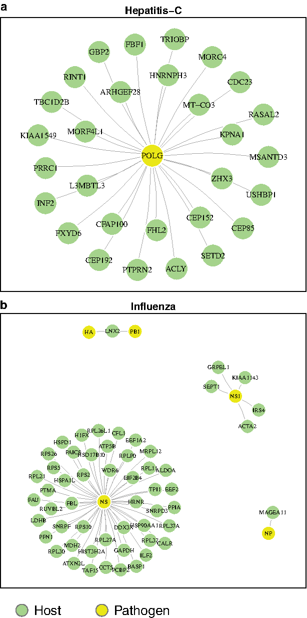
Disadvantages of the Homolog method: In Figure 3, we show for two tasks the protein interactions in the test data (for one train–test split) that were not found by the Homolog model that relies purely on homology-based sequence similarity.
PPIs from each task that are found by our method but are missed by the homolog method. These are those for which sequence-similar proteins were not found. (a)Hepatitis-C–human PPI and (b)Influenza–human PPI. PPI, protein–protein interaction.
6.1. Biological significance of the model
The model parameters U, V, and S are a source of rich information that can be used to further understand host–pathogen interactions. Note that our features are derived from the amino acid sequences of the proteins that provide opportunities to interpret the parameters.
1. Clustering proteins based on interaction propensities: We analyze the proteins by projecting them using the model parameters U and V into a lower dimensional subspace (i.e., computing \documentclass{aastex}\usepackage{amsbsy}\usepackage{amsfonts}\usepackage{amssymb}\usepackage{bm}\usepackage{mathrsfs}\usepackage{pifont}\usepackage{stmaryrd}\usepackage{textcomp}\usepackage{portland, xspace}\usepackage{amsmath, amsxtra}\usepackage{upgreek}\pagestyle{empty}\DeclareMathSizes{10}{9}{7}{6}\begin{document}
$$XU^{ \rm T}$$
\end{document} and \documentclass{aastex}\usepackage{amsbsy}\usepackage{amsfonts}\usepackage{amssymb}\usepackage{bm}\usepackage{mathrsfs}\usepackage{pifont}\usepackage{stmaryrd}\usepackage{textcomp}\usepackage{portland, xspace}\usepackage{amsmath, amsxtra}\usepackage{upgreek}\pagestyle{empty}\DeclareMathSizes{10}{9}{7}{6}\begin{document}
$$YV^{ \rm T}$$
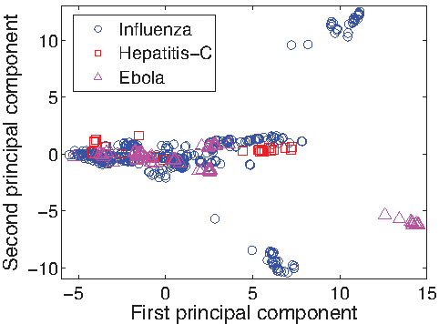
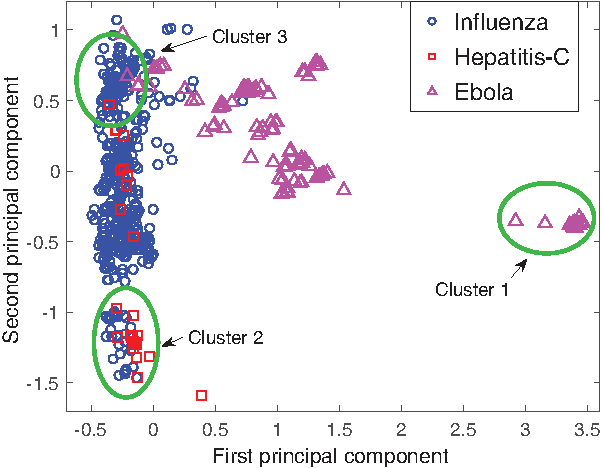
\end{document} to get projections of the virus and human proteins, respectively). The principal component analysis (PCA) of this lower dimensional representation is compared with PCA in the original feature space (protein sequence features) in Figures 1 and 2. First, the projected data have a much better separation than the original data. Second, Figure 2 shows that Hepatitis-C and Influenza have many proteins with similar binding tendencies, and that these behave differently than most Ebola virus proteins. This observation is not obvious in the PCA of the original feature space (Fig. 1), in which proteins with similar sequences group together. We analyze the projected data further by looking at the clusters of proteins for enrichment of GO3 (Ashburner et al., 2000) annotations (proteins were first clustered in this lower dimensional space using k-means and setting the number of clusters to 6). Of particular interest are the highlighted three clusters that contain either proteins projected far from others (such as cluster 1) or proteins from different viruses projected close together (cluster 2 and cluster 3). For enrichment analysis, we use the FuncAssociate 3.04 (Berriz et al., 2003) tool and GO annotations for the three viruses from UniProtKB.
2. Novel interactions with Ebola proteins: The top four Ebola–human PPIs are all predictions for the Ebola envelope glycoprotein (GP) with four different human proteins (Note: GP is not in the gold standard PPIs). There is abundant evidence in the published literature (Nanbo et al., 2010) for the critical role played by GP in virus docking and fusion with the host cell.
3. Sequence motifs from virus proteins: We analyze sequence motifs derived from the top k-mers that contribute to interactions. The significant entries of the model parameters U, V, and \documentclass{aastex}\usepackage{amsbsy}\usepackage{amsfonts}\usepackage{amssymb}\usepackage{bm}\usepackage{mathrsfs}\usepackage{pifont}\usepackage{stmaryrd}\usepackage{textcomp}\usepackage{portland, xspace}\usepackage{amsmath, amsxtra}\usepackage{upgreek}\pagestyle{empty}\DeclareMathSizes{10}{9}{7}{6}\begin{document}
$$\{ {S_t} \} $$
\end{document} were used to compute these motifs. The top positive-valued entries from the product \documentclass{aastex}\usepackage{amsbsy}\usepackage{amsfonts}\usepackage{amssymb}\usepackage{bm}\usepackage{mathrsfs}\usepackage{pifont}\usepackage{stmaryrd}\usepackage{textcomp}\usepackage{portland, xspace}\usepackage{amsmath, amsxtra}\usepackage{upgreek}\pagestyle{empty}\DeclareMathSizes{10}{9}{7}{6}\begin{document}
$$U{V^T}$$
\end{document} indicate which pairs of features (\documentclass{aastex}\usepackage{amsbsy}\usepackage{amsfonts}\usepackage{amssymb}\usepackage{bm}\usepackage{mathrsfs}\usepackage{pifont}\usepackage{stmaryrd}\usepackage{textcomp}\usepackage{portland, xspace}\usepackage{amsmath, amsxtra}\usepackage{upgreek}\pagestyle{empty}\DeclareMathSizes{10}{9}{7}{6}\begin{document}
$$( {f_v} , {f_h} )$$
\end{document}: virus protein feature, human protein feature) are important for interactions across all the virus–human PPI tasks. Analogously, the entries from St give us pairs of features important to a particular virus–human task “t”. These results are given in the Supplementary Data.
Principal component analysis (PCA) of virus proteins in the original feature space. The first two principal components are shown. Shape and color of the points indicate which virus that protein comes from.
PCA of virus proteins in the projected subspace. The first two principal components are shown. Shape of the points indicates which virus that protein comes from. We have highlighted three clusters for which we show gene ontology term enrichment analysis results in Table 5.
Gene Ontology Terms (for Process, Function, Component) Enriched in the Highlighted Clusters fromFigure 2
mRNA (guanine-N7-)-methyltransferase activity; RNA-directed RNA polymerase activity; ATP binding
Cluster 2 (hepatitis and influenza proteins)
Host cell endoplasmic reticulum membrane; host cell lipid particle; induction by virusof host autophagy; host cell mitochondrial membrane; suppression by virus of host STAT1 activity
Cluster 3 (all)
Fusion of virus membrane with host plasma membrane
FuncAssociate GO enrichment tool4 was used and terms with p < 0.001 are shown. The first column also indicates the composition of each cluster (i.e., which task's proteins appear in the cluster).
7. Conclusions and Future Extensions
This work developed and tested a new multitask learning method for HP PPI prediction based on low-rank matrix completion for sharing information across tasks. Our method, BSL-MTL, exhibited large increases in prediction accuracy compared with a variety of baselines. The model parameters provide several avenues for further studying HP PPI that can lead to interesting observations and insights. Finally, the model we present is general enough to be applicable on other problems such as gene–disease relevance prediction across organisms or disease conditions.
Footnotes
Author Disclosure Statement
No conflicting financial interests exist.
References
1.
AbernethyJ., BachF., EvgeniouT., and VertJ.P. (2009). A new approach to collaborative filtering: Operator estimation with spectral regularization. J. Mach. Learn. Res., 10, 803–826.
2.
AndoR.K., and ZhangT. (2005). A framework for learning predictive structures from multiple tasks and unlabeled data. J. Mach. Learn. Res., 6, 1817–1853.
3.
AshburnerM., BallC.A., BlakeJ.A., et al. (2000). Gene ontology: Tool for the unification of biology. Nat. Gene., 25, 25–29.
4.
BerrizG., KingO., BryantB., et al. (2003). Characterizing gene sets with funcassociate. Bioinformatics, 19, 2502–2504.
5.
CandesE., and RechtB. (2009). Exact matrix completion via convex optimization. Found. Comput. Math., 9, 717.
6.
CaoB., LiuN.N., and YangQ. (2010). Transfer learning for collective link prediction in multiple heterogenous domains. In International Conference on Machine Learning, 159–166.
7.
ChatraryamontriA., CeolA., PelusoD., et al. (2009). Virusmint: A viral protein interaction database. Nucleic Acids Res., 37, D669–D673.
8.
ChenC.-C., LinC.-Y., LoY.-S., and YangJ.-M. (2009). Ppisearch: A web server for searching homologous protein–protein interactions across multiple species. Nucleic Acids Res., 37(suppl 2), W369–W375.
9.
ChenJ., LiuJ., and YeJ. (2012). Learning incoherent sparse and low-rank patterns from multiple tasks. ACM Trans. Knowl. Discov. Data, 5, 22.
10.
ChenJ., TangL., LiuJ., and YeJ. (2013). A convex formulation for learning a shared predictive structure from multiple tasks. IEEE Trans. Pattern Anal. Mach. Intell., 35, 1025–1038.
11.
ChenX., and LiuM. (2005). Prediction of protein-protein interactions using random decision forest framework. Bioinformatics, 21, 4394–4400.
12.
DavisJ., and GoadrichM. (2006). The relationship between precision-recall and roc curves. In Proceedings of the 23rd International Conference on Machine Learning, 233–240.
13.
DyerM., MuraliT., and SobralB. (2007). Computational prediction of host-pathogen protein-protein interactions. Bioinformatics, 23, i159–66.
14.
DyerM., MuraliT.M., SobralB.W. (2011). Supervised learning and prediction of physical interactions between human and hiv proteins. Infect. Genet. Evol., 11, 917–923.
15.
EvgeniouT., and PontilM. (2004). Regularized multi-task learning. In Proceedings of the 10th ACM SIGKDD International Conference on Knowledge Discovery and Data Mining, 109–117.
JiS., and YeJ. (2009). An accelerated gradient method for trace norm minimization. In Proceedings of the 26th Annual International Conference on Machine Learning, 457–464. ACM.
18.
JinR., SiL., and ZhaiC. (2002). Preference-based graphic models for collaborative filtering. 329–336, In Proceedings of the 19th Conference on Uncertainty in Artificial Intelligence, Morgan Kaufmann Publishers Inc.
19.
KorenY., BellR., and VolinskyC. (2009). Matrix factorization techniques for recommender systems. IEEE Comput., 42, 30–37.
20.
KshirsagarM., CarbonellJ.G., and Klein-SeetharamanJ. (2012). Techniques to cope with missing data in host-pathogen protein interaction prediction. Bioinformatics, 28, i466–i472.
21.
KshirsagarM., CarbonellJ.G., and Klein-SeetharamanJ. (2013). Multi-task learning for host-pathogen protein interactions. Bioinformatics, 29, i217–i226.
22.
KumarR., and NanduriB. (2010). Hpidb—A unified resource for host-pathogen interactions. BMC Bioinformatics, 11(Suppl 6), S16.
23.
LiB., YangQ., and XueX. (2009). Transfer learning for collaborative filtering via a rating-matrix generative model. In International Conference on Machine Learning, 617–624. ACM.
24.
LinC.-Y., ChenY.-C., LoY.-S., and YangJ.-M. (2013). Inferring homologous protein-protein interactions through pair position specific scoring matrix. BMC Bioinformatics, 14, 1.
25.
MatthewsL.R., VaglioP., ReboulJ., GeH., DavisB.P., GarrelsJ., VincentS., and VidalM. (2001). Identification of potential interaction networks using sequence-based searches for conserved protein-protein interactions or interologs. Genome Res., 11, 2120–2126.
26.
MenonA.K., and ElkanC. (2011). Link prediction via matrix factorization. Joint European Conference on Machine Learning and Knowledge Discovery in Databases, 437–452.
27.
MikaS., and RostB. (2006). Protein–protein interactions more conserved within species than across species. PLoS Comput. Biol., 2, e79.
28.
MirzazadehF., WhiteM., GyörgyA., and SchuurmansD. (2015). Scalable metric learning for co-embedding. In Joint European Conference on Machine Learning and Knowledge Discovery in Databases (ECML-KDD), 625–642. Springer.
29.
MurakamiY. and MizuguchiK. (2014). Homology-based prediction of interactions between proteins using averaged one-dependence estimators. BMC Bioinformatics, 15, 213.
30.
NanboA., ImaiM., WatanabeS., et al. (2010). Ebolavirus is internalized into host cells via macropinocytosis in a viral glycoprotein-dependent manner. PLoS Pathog., 6, e1001121.
31.
NatarajanN., and DhillonI.S. (2014). Inductive matrix completion for predicting gene–disease associations. Bioinformatics, 30, i60–i68.
32.
PhungD.Q., VenkateshS., et al. (2009). Ordinal boltzmann machines for collaborative filtering. In UAI, 548–556. AUAI Press.
33.
QiY., Bar-JosephZ., Klein-SeetharamanJ. (2006). Evaluation of different biological data and computational classification methods for use in protein interaction prediction. Proteins, 63, 490–500.
34.
QiY., DhimanH., Bar-JosephZ., et al. (2009). Systematic prediction of human membrane receptor interactions. Proteomics, 23, 5243–55.
35.
QiY., TastanO., CarbonellJ.G., Klein-SeetharamanJ., and WestonJ. (2010). Semi-supervised multi-task learning for predicting interactions between HIV-1 and human proteins. Bioinformatics, 26, i645–i652.
36.
SarwarB., KarypisG., KonstanJ., and RiedlJ. (2001). Item-based collaborative filtering recommendation algorithms. In Proceedings of the 10th International Conference on World Wide Web, 285–295. ACM.
37.
ShenJ., ZhangJ., LuoX., et al. (2007). Predicting protein-protein interactions based only on sequences information. Proc. Natl. Acad. Sci. U. S. A., 104, 4337–4341.
38.
SinghA.P., and GordonG.J. (2008). Relational learning via collective matrix factorization. In Proceedings of the 14th ACM SIGKDD International Conference on Knowledge Discovery and Data Mining, 650–658.
39.
SinghR., XuJ., and BergerB. (2006). Struct2net: Integrating structure into protein-protein interaction prediction. Pac. Symp. Biocomput., 11, 403–411.
40.
TastanO., QiY., CarbonellJ.G., et al. (2009). Prediction of interactions between hiv-1 and human proteins by information integration. Pac. Symp. Biocomput.516–527.
41.
TekirS.D., CakirT., and UlgenK.Ö. (2012). Infection strategies of bacterial and viral pathogens through pathogen-human protein protein interactions. Syst. Biol. Microb. Infect., 3, 74.
42.
UniProt Consortium (2011). Ongoing and future developments at the universal protein resource. Nucleic Acids Res., 39, D214–D219.
43.
WalhoutA.J., and VidalM. (2001). Protein interaction maps for model organisms. Nat. Rev. Mol. Cell Biol., 2, 55–63.
44.
WuX., ZhuL., GuoJ., et al. (2006). Prediction of yeast protein-protein interaction network: Insights from the gene ontology and annotations. Nucleic Acids Res., 34, 2137–2150.
45.
XuQ., XiangE.W., and YangQ. (2010). Protein-protein interaction prediction via collective matrix factorization. In International Conference on Bioinformatics and Biomedicine.
ZhouJ., ChenJ., and YeJ. (2011). MALSAR: Multi-task Learning via Structural Regularization. Arizona State University.
Supplementary Material
Please find the following supplemental material available below.
For Open Access articles published under a Creative Commons License, all supplemental material carries the same license as the article it is associated with.
For non-Open Access articles published, all supplemental material carries a non-exclusive license, and permission requests for re-use of supplemental material or any part of supplemental material shall be sent directly to the copyright owner as specified in the copyright notice associated with the article.