pSuc-PseRat: Predicting Lysine Succinylation in Proteins by Exploiting the Ratios of Sequence Coupling and Properties

Abstract

Lysine succinylation is an extremely important protein post-translational modification that plays a fundamental role in regulating various biological reactions, and dysfunction of this process is associated with a number of diseases. Thus, determining which Lys residues in an uncharacterized protein sequence are succinylated underpins both basic research and drug development endeavors. To solve this problem, we have developed a predictor called pSuc-PseRat. The features of the pSuc-PseRat predictor are derived from two aspects: (1) the binary encoding from succinylated sites and non-succinylated sites; (2) the sequence-coupling effects between succinylated sites and non-succinylated sites. Eleven gradient boosting machine classifiers were trained with these features to build the predictor. The pSuc-PseRat predictor achieved an average ACU (area under the receiver operating characteristic curve) score of 0.805 in the fivefold cross-validation set and performed better than existing predictors on two comprehensive independent test sets. A freely available web server has been developed for pSuc-PseRat.

1. Introduction

An efficient biological mechanism for expanding the genetic code and regulating cell physiology is post-translational modification (PTM) of proteins (Walsh et al., 2005). As a type of PTM, lysine succinylation was identified initially by mass spectrometry and protein sequence alignment (Zhang et al., 2011). Further studies showed that lysine succinylation promotes remarkable changes in protein structure and function (Zhang et al., 2011; Xie et al., 2012). Park et al. (2013) identified 2565 succinylation sites on 779 proteins and revealed that lysine succinylation of enzymes has potential effects on mitochondrial metabolism, including amino acid degradation, the tricarboxylic acid cycle (TCA), and fatty acid metabolism. Consequently, the identification of succinylated sites in proteins should provide useful information for both basic research and drug development.

Identification of the amino acids with PTMs was primarily performed by mass spectrometry, which can be both expensive and laborious. Consequently, the development of computational methods represents an ideal approach to overcome these experimental shortcomings. Three computational methods have been proposed for prediction of succinylation sites (Xu et al., 2015a,b; Hasan et al., 2016). Xu et al. (2015b) developed a support vector machine (SVM)-based predictor named iSuc-PseAAC by incorporating the peptide position-specific propensity into the general form of a pseudo amino acid composition. After iSuc-PseAAC, Xu et al. also developed a SVM-based predictor named SuccFind. This predictor was constructed to predict lysine succinylation sites based on two major features: (1) sequence-derived features; (2) evolutionary-derived information of the sequence (Xu et al., 2015a). More recently, Hasan et al. (2016) developed another predictor named SuccinSite, which is based on the random forest classifier to predict protein succinylation sites by incorporating three sequence encodings, that is, k-spaced amino acid pairs, binary and amino acid index properties.

Nevertheless, the performance of the predictors can be improved. First, the iSuc-PseAAC predictor datasets were compiled from the lysine modification database (Liu et al., 2014) and the SuccFind predictor dataset was compiled from the lysine modification database and some relevant articles (Liu et al., 2014; Park et al., 2013; Li et al., 2014). The training datasets of these two predictors are relatively small and likely miss many novel succinylation sites from the latest high-throughput proteomic assays. Second, although SuccinSite uses several new datasets from published articles (Zhang et al., 2011; Colak et al., 2013; Park et al., 2013; Weinert et al., 2013; Li et al., 2014; Yang et al., 2015), there remain problems in the formation of its training set. After applying a 30% homology-reducing screening procedure with CD-HIT (Huang et al., 2010), 5004 experimentally verified lysine succinylation sites were obtained as positive samples (i.e., succinylated sites) and all the remaining lysine residues were obtained as negative samples (i.e., non-succinylated sites) (Hasan et al., 2016). In this article, ∼80% of the negative dataset was ignored, suggesting that this approach might lead to the negative training data omitting some useful information. Finally, each investigated succinylated or non-succinylated fragment was encoded as a high-dimensional vector, and the feature selection method could influence the classification of the SVM and random forest model.

To improve the predictive performance in this study, we proposed a novel predictor “‘pSuc-PseRat” for the prediction of lysine succinylation sites. First, we compiled a more comprehensive dataset containing 12,356 lysine succinylation sites from 4411 proteins and the selection of the training set was more reasonable than the SuccFind predictor and the iSuc-PseAAC predictor. Second, the Proportion of Amino Acid Pairs Positions (PAAPP) matrices [Eq. (10)] were introduced to make the feature description more complete. Finally, gradient boosting machine (GBM) classifiers were used, which contain an implicit feature selection method.

2. Materials and Methods

2.1. Benchmark dataset

The annotations of succinylated sites used in this study were collected from published articles (Zhang et al., 2011; Colak et al., 2013; Park et al., 2013; Weinert et al., 2013; Li et al., 2014; Yang et al., 2015). This information of succinylated proteins was derived from the UniProtKB/Swiss-Prot (Hunter et al., 2012) and NCBI protein sequence database (www.ncbi.nlm.nih.gov/protein). In these collections of succinylated proteins, some proteins were not present in the protein sequence database and some protein lysine positions did not match with the position in the database. Consequently, these proteins were removed from our study. There were 14,591 lysine succinylation sites and 96,114 non-succinylation sites in 4960 unique proteins. For facilitating the description later, Chou's peptide formulation was applied in this article. Chou's peptide formulation was used for signal peptide cleavage sites (Boeckmann et al., 2003) and S-nitrosylation site prediction (Xu et al., 2013).

According to Chou's scheme, a peptide with a lysine (K) located at its center can be expressed as \documentclass{aastex}\usepackage{amsbsy}\usepackage{amsfonts}\usepackage{amssymb}\usepackage{bm}\usepackage{mathrsfs}\usepackage{pifont}\usepackage{stmaryrd}\usepackage{textcomp}\usepackage{portland, xspace}\usepackage{amsmath, amsxtra}\usepackage{upgreek}\pagestyle{empty}\DeclareMathSizes{10}{9}{7}{6}\begin{document} \begin{align*} { \it{P}} = {R_{ - \xi }}{R_{ - \left( { \xi - 1} \right) }} \cdots {R_{ - 2}}{R_{ - 1}} \mathbb{K}{R_{ + 1}}{R_{ + 2}} \cdots {R_{ + \left( { \xi - 1} \right) }}{R_{ + \xi }} \tag{1} \end{align*} \end{document}

where the subscript ξ represents an integer, R_−ξ represents the ξ-th downstream amino acid residue from the center, and R_+ξ represents the ξ-th upstream amino acid residue. A peptide P can be defined by the following two categories: \documentclass{aastex}\usepackage{amsbsy}\usepackage{amsfonts}\usepackage{amssymb}\usepackage{bm}\usepackage{mathrsfs}\usepackage{pifont}\usepackage{stmaryrd}\usepackage{textcomp}\usepackage{portland, xspace}\usepackage{amsmath, amsxtra}\usepackage{upgreek}\pagestyle{empty}\DeclareMathSizes{10}{9}{7}{6}\begin{document} \begin{align*} P \in \begin{cases} P_ \xi ^ + \left( \mathbb{K} \right) , & { \rm{if \ its \ center \ is \ a \ succinylation \ site}} \\ P_ \xi ^ - \left( \mathbb{K} \right) , & { \rm{otherwise}} \end{cases} \tag{2} \end{align*} \end{document}

Thus, the benchmark dataset can be formulated as: \documentclass{aastex}\usepackage{amsbsy}\usepackage{amsfonts}\usepackage{amssymb}\usepackage{bm}\usepackage{mathrsfs}\usepackage{pifont}\usepackage{stmaryrd}\usepackage{textcomp}\usepackage{portland, xspace}\usepackage{amsmath, amsxtra}\usepackage{upgreek}\pagestyle{empty}\DeclareMathSizes{10}{9}{7}{6}\begin{document} \begin{align*} \mathbb{S} = { \mathbb{S}^ + } \cup { \mathbb{S}^ - } \tag{3} \end{align*} \end{document}

In this study, the parameter ξ in peptides was set to 13 after some preliminary trials, and the sample extracted from proteins was a 2ξ + 1 = 27 tuple peptide. If the upstream or downstream sequence in a peptide sample was less than ξ, the residual part was replaced by a dummy code X. Peptides that had ≥40% pairwise sequence identity to any other peptide [calculated by CD-HIT (Huang et al., 2010)] were rigorously excluded from the benchmark dataset.

Finally, we obtained the benchmark dataset \documentclass{aastex}\usepackage{amsbsy}\usepackage{amsfonts}\usepackage{amssymb}\usepackage{bm}\usepackage{mathrsfs}\usepackage{pifont}\usepackage{stmaryrd}\usepackage{textcomp}\usepackage{portland, xspace}\usepackage{amsmath, amsxtra}\usepackage{upgreek}\pagestyle{empty}\DeclareMathSizes{10}{9}{7}{6}\begin{document} $$\mathbb{S}$$ \end{document} with 33,703 peptides. The center of these peptides contained 7047 experimentally verified lysine succinylation sites in \documentclass{aastex}\usepackage{amsbsy}\usepackage{amsfonts}\usepackage{amssymb}\usepackage{bm}\usepackage{mathrsfs}\usepackage{pifont}\usepackage{stmaryrd}\usepackage{textcomp}\usepackage{portland, xspace}\usepackage{amsmath, amsxtra}\usepackage{upgreek}\pagestyle{empty}\DeclareMathSizes{10}{9}{7}{6}\begin{document} $${ \mathbb{S}^ + }$$ \end{document} and 26,656 non-succinylated sites in \documentclass{aastex}\usepackage{amsbsy}\usepackage{amsfonts}\usepackage{amssymb}\usepackage{bm}\usepackage{mathrsfs}\usepackage{pifont}\usepackage{stmaryrd}\usepackage{textcomp}\usepackage{portland, xspace}\usepackage{amsmath, amsxtra}\usepackage{upgreek}\pagestyle{empty}\DeclareMathSizes{10}{9}{7}{6}\begin{document} $${ \mathbb{S}^ - }$$ \end{document} . The independent test set can be formulated as: \documentclass{aastex}\usepackage{amsbsy}\usepackage{amsfonts}\usepackage{amssymb}\usepackage{bm}\usepackage{mathrsfs}\usepackage{pifont}\usepackage{stmaryrd}\usepackage{textcomp}\usepackage{portland, xspace}\usepackage{amsmath, amsxtra}\usepackage{upgreek}\pagestyle{empty}\DeclareMathSizes{10}{9}{7}{6}\begin{document} \begin{align*} \mathbb{I} = { \mathbb{I}^ + } \cup { \mathbb{I}^ - } \tag{4} \end{align*} \end{document}

We took the remaining 90% part of \documentclass{aastex}\usepackage{amsbsy}\usepackage{amsfonts}\usepackage{amssymb}\usepackage{bm}\usepackage{mathrsfs}\usepackage{pifont}\usepackage{stmaryrd}\usepackage{textcomp}\usepackage{portland, xspace}\usepackage{amsmath, amsxtra}\usepackage{upgreek}\pagestyle{empty}\DeclareMathSizes{10}{9}{7}{6}\begin{document} $$\mathbb{S}$$ \end{document} as the training set, which can be formulated as: \documentclass{aastex}\usepackage{amsbsy}\usepackage{amsfonts}\usepackage{amssymb}\usepackage{bm}\usepackage{mathrsfs}\usepackage{pifont}\usepackage{stmaryrd}\usepackage{textcomp}\usepackage{portland, xspace}\usepackage{amsmath, amsxtra}\usepackage{upgreek}\pagestyle{empty}\DeclareMathSizes{10}{9}{7}{6}\begin{document} \begin{align*} \mathbb{T} = { \mathbb{T}^ + } \cup { \mathbb{T}^ - } \tag{5} \end{align*} \end{document}

It should be noted that the number of \documentclass{aastex}\usepackage{amsbsy}\usepackage{amsfonts}\usepackage{amssymb}\usepackage{bm}\usepackage{mathrsfs}\usepackage{pifont}\usepackage{stmaryrd}\usepackage{textcomp}\usepackage{portland, xspace}\usepackage{amsmath, amsxtra}\usepackage{upgreek}\pagestyle{empty}\DeclareMathSizes{10}{9}{7}{6}\begin{document} $${ \mathbb{T}^ - }$$ \end{document} was nearly four times as much as \documentclass{aastex}\usepackage{amsbsy}\usepackage{amsfonts}\usepackage{amssymb}\usepackage{bm}\usepackage{mathrsfs}\usepackage{pifont}\usepackage{stmaryrd}\usepackage{textcomp}\usepackage{portland, xspace}\usepackage{amsmath, amsxtra}\usepackage{upgreek}\pagestyle{empty}\DeclareMathSizes{10}{9}{7}{6}\begin{document} $${ \mathbb{T}^ + }$$ \end{document} , so \documentclass{aastex}\usepackage{amsbsy}\usepackage{amsfonts}\usepackage{amssymb}\usepackage{bm}\usepackage{mathrsfs}\usepackage{pifont}\usepackage{stmaryrd}\usepackage{textcomp}\usepackage{portland, xspace}\usepackage{amsmath, amsxtra}\usepackage{upgreek}\pagestyle{empty}\DeclareMathSizes{10}{9}{7}{6}\begin{document} $$\mathbb{T}$$ \end{document} was an unbalanced dataset. To solve this problem, we used the following method: The predictors were trained with different training sets, and the prediction results of these predictors were averaged as the final prediction. We also explored the impact of the number of predictors on model performance in Table 1. We used the area under ROC curve (AUC) as the evaluation criterion and found that the number of predictors reached the best value when the number was 10 and 11. When the number continued to increase, AUC began to decrease, so we chose 11 as the total number of predictors. We kept the full \documentclass{aastex}\usepackage{amsbsy}\usepackage{amsfonts}\usepackage{amssymb}\usepackage{bm}\usepackage{mathrsfs}\usepackage{pifont}\usepackage{stmaryrd}\usepackage{textcomp}\usepackage{portland, xspace}\usepackage{amsmath, amsxtra}\usepackage{upgreek}\pagestyle{empty}\DeclareMathSizes{10}{9}{7}{6}\begin{document} $${ \mathbb{T}^ + }$$ \end{document} -positive training data and from \documentclass{aastex}\usepackage{amsbsy}\usepackage{amsfonts}\usepackage{amssymb}\usepackage{bm}\usepackage{mathrsfs}\usepackage{pifont}\usepackage{stmaryrd}\usepackage{textcomp}\usepackage{portland, xspace}\usepackage{amsmath, amsxtra}\usepackage{upgreek}\pagestyle{empty}\DeclareMathSizes{10}{9}{7}{6}\begin{document} $${ \mathbb{T}^ - }$$ \end{document} a subset of 6343 sites were selected randomly. The 11 selected negative datasets were defined as \documentclass{aastex}\usepackage{amsbsy}\usepackage{amsfonts}\usepackage{amssymb}\usepackage{bm}\usepackage{mathrsfs}\usepackage{pifont}\usepackage{stmaryrd}\usepackage{textcomp}\usepackage{portland, xspace}\usepackage{amsmath, amsxtra}\usepackage{upgreek}\pagestyle{empty}\DeclareMathSizes{10}{9}{7}{6}\begin{document} $$\mathbb{T}_1^ - , \mathbb{T}_2^ - , \cdots , \mathbb{T}_{11}^ -$$ \end{document} , \documentclass{aastex}\usepackage{amsbsy}\usepackage{amsfonts}\usepackage{amssymb}\usepackage{bm}\usepackage{mathrsfs}\usepackage{pifont}\usepackage{stmaryrd}\usepackage{textcomp}\usepackage{portland, xspace}\usepackage{amsmath, amsxtra}\usepackage{upgreek}\pagestyle{empty}\DeclareMathSizes{10}{9}{7}{6}\begin{document} $${ \mathbb{T}^ + }$$ \end{document} and \documentclass{aastex}\usepackage{amsbsy}\usepackage{amsfonts}\usepackage{amssymb}\usepackage{bm}\usepackage{mathrsfs}\usepackage{pifont}\usepackage{stmaryrd}\usepackage{textcomp}\usepackage{portland, xspace}\usepackage{amsmath, amsxtra}\usepackage{upgreek}\pagestyle{empty}\DeclareMathSizes{10}{9}{7}{6}\begin{document} $$\mathbb{T}_i^ - \left( {i = 1 , 2 \cdots 11} \right)$$ \end{document} as the balanced datasets for the 11-model prediction.

Table 1.

The Training Set [ Eq. (10) ] Performances of the GBM Classifiers with Fivefold Cross-validation, GBM[i], i = 1, 2, 3…, 11; the “i” Presents the Total Number of the GBM Classifiers in the Experiment

	AUC	Sen	Spe	Acc	MCC
GBM[1]	0.738	0.682	0.664	0.668	0.287
GBM[2]	0.743	0.527	0.802	0.744	0.302
GBM[3]	0.754	0.705	0.669	0.677	0.309
GBM[4]	0.759	0.713	0.680	0.687	0.326
GBM[5]	0.760	0.717	0.678	0.686	0.328
GBM[6]	0.764	0.722	0.679	0.688	0.331
GBM[7]	0.765	0.717	0.680	0.688	0.330
GBM[8]	0.765	0.709	0.683	0.689	0.326
GBM[9]	0.765	0.709	0.680	0.686	0.322
GBM[10]	0.767	0.707	0.682	0.687	0.323
GBM[11]	0.767	0.706	0.680	0.686	0.321
GBM[12]	0.763	0.724	0.664	0.676	0.320
GBM[13]	0.763	0.700	0.685	0.688	0.321

Acc, accuracy; GBM, gradient boosting machine; Spe, specificity; Sen, sensitivity; MCC, the Matthews correlation coefficient; AUC, area under the receiver operating characteristic curve.

As some peptide samples in \documentclass{aastex}\usepackage{amsbsy}\usepackage{amsfonts}\usepackage{amssymb}\usepackage{bm}\usepackage{mathrsfs}\usepackage{pifont}\usepackage{stmaryrd}\usepackage{textcomp}\usepackage{portland, xspace}\usepackage{amsmath, amsxtra}\usepackage{upgreek}\pagestyle{empty}\DeclareMathSizes{10}{9}{7}{6}\begin{document} $$\mathbb{I}$$ \end{document} were repeated in the training set of SuccinSite (Xu et al., 2015b), we used another independent test set \documentclass{aastex}\usepackage{amsbsy}\usepackage{amsfonts}\usepackage{amssymb}\usepackage{bm}\usepackage{mathrsfs}\usepackage{pifont}\usepackage{stmaryrd}\usepackage{textcomp}\usepackage{portland, xspace}\usepackage{amsmath, amsxtra}\usepackage{upgreek}\pagestyle{empty}\DeclareMathSizes{10}{9}{7}{6}\begin{document} $$\mathbb{I} ^\prime$$ \end{document} for a comparison of the performances between SuccinSite and pSuc-PseRat. The dataset \documentclass{aastex}\usepackage{amsbsy}\usepackage{amsfonts}\usepackage{amssymb}\usepackage{bm}\usepackage{mathrsfs}\usepackage{pifont}\usepackage{stmaryrd}\usepackage{textcomp}\usepackage{portland, xspace}\usepackage{amsmath, amsxtra}\usepackage{upgreek}\pagestyle{empty}\DeclareMathSizes{10}{9}{7}{6}\begin{document} $$\mathbb{I} ^\prime$$ \end{document} was derived from iSuc-PseAAC (Xu et al., 2015b); this set contained 4720 peptide samples and was formulated as \documentclass{aastex}\usepackage{amsbsy}\usepackage{amsfonts}\usepackage{amssymb}\usepackage{bm}\usepackage{mathrsfs}\usepackage{pifont}\usepackage{stmaryrd}\usepackage{textcomp}\usepackage{portland, xspace}\usepackage{amsmath, amsxtra}\usepackage{upgreek}\pagestyle{empty}\DeclareMathSizes{10}{9}{7}{6}\begin{document} \begin{align*} \mathbb{I}^ \prime = { \mathbb{I}^{ \prime + }} \cup { \mathbb{I}^{ \prime - }} \tag{6} \end{align*} \end{document}

2.2. Feature vector construction

2.2.1. Construction of score matrix

Protein sequences provided the most important information to construct the feature, and the peptides were converted into effective mathematical expressions that could reflect intrinsic correlations with the desired target in predicting the PTMs (Chou, 2011). To select the best window size, five ensemble GBM classifiers were trained with different window sizes. The performance of these models was evaluated by using independent test set \documentclass{aastex}\usepackage{amsbsy}\usepackage{amsfonts}\usepackage{amssymb}\usepackage{bm}\usepackage{mathrsfs}\usepackage{pifont}\usepackage{stmaryrd}\usepackage{textcomp}\usepackage{portland, xspace}\usepackage{amsmath, amsxtra}\usepackage{upgreek}\pagestyle{empty}\DeclareMathSizes{10}{9}{7}{6}\begin{document} $$\mathbb{I}$$ \end{document} , and the results are shown in Table 2. It can be seen that there were small improvements in the value of AUC when the window size was increased from 21 to 27. The value of AUC almost no longer changed when the window size was greater than 27. Therefore, we selected 27 as the optimum window size in this study. Clearly, Equation (1) showed that when ξ = 13, the corresponding peptide contains (2ξ + 1) = 27 amino acid residues. A peptide P′ could be reduced to \documentclass{aastex}\usepackage{amsbsy}\usepackage{amsfonts}\usepackage{amssymb}\usepackage{bm}\usepackage{mathrsfs}\usepackage{pifont}\usepackage{stmaryrd}\usepackage{textcomp}\usepackage{portland, xspace}\usepackage{amsmath, amsxtra}\usepackage{upgreek}\pagestyle{empty}\DeclareMathSizes{10}{9}{7}{6}\begin{document} \begin{align*} { \it{P ^\prime }} = {R_1}{R_2} \cdots {R_{13}}{R_{14}}{R_{15}} \cdots {R_{26}}{R_{27}} \tag{7} \end{align*} \end{document}

Table 2.

The Performances of Different Processing Methods for Imbalanced Datasets with the Independent Test Set

Window size	AUC	Sen	Sep	Acc	MCC
21	0.763	0.618	0.768	0.737	0.339
23	0.765	0.626	0.767	0.737	0.343
25	0.766	0.676	0.718	0.710	0.333
27	0.767	0.706	0.680	0.686	0.321
29	0.767	0.705	0.682	0.697	0.319
31	0.767	0.708	0.678	0.681	0.323

where the superscript l was the distance between R_i and \documentclass{aastex}\usepackage{amsbsy}\usepackage{amsfonts}\usepackage{amssymb}\usepackage{bm}\usepackage{mathrsfs}\usepackage{pifont}\usepackage{stmaryrd}\usepackage{textcomp}\usepackage{portland, xspace}\usepackage{amsmath, amsxtra}\usepackage{upgreek}\pagestyle{empty}\DeclareMathSizes{10}{9}{7}{6}\begin{document} $${R_j}\ \left( {i = 1 , 2 , \cdots , 27;j = 1 , 2 , \cdots , 27 \ and \ i \ne j} \right)$$ \end{document} , so the value of l could be selected from 1 to 26, the element \documentclass{aastex}\usepackage{amsbsy}\usepackage{amsfonts}\usepackage{amssymb}\usepackage{bm}\usepackage{mathrsfs}\usepackage{pifont}\usepackage{stmaryrd}\usepackage{textcomp}\usepackage{portland, xspace}\usepackage{amsmath, amsxtra}\usepackage{upgreek}\pagestyle{empty}\DeclareMathSizes{10}{9}{7}{6}\begin{document} \begin{align*} z_{i , j}^l = \left\{ \begin{matrix} \qquad 0 , \qquad\quad when \ F_{i , j}^{l + } = 0 \ and \ F_{i , j}^{l - } = 0 \hfill \\ \qquad 1 , \qquad\quad when \ F_{i , j}^{l + } \ne 0 \ and \ F_{i , j}^{l - } = 0 \hfill \\ \qquad - 1 , \qquad when \ F_{i , j}^{l + } = 0 \ and \ F_{i , j}^{l - } \ne 0 \hfill \\ 1 - F_{i , j}^{l - } / F_{i , j}^{l + } , \ \qquad when \ F_{i , j}^{l + } \ge F_{i , j}^{l - } > 0 \hfill \\ 1 - F_{i , j}^{l + } / F_{i , j}^{l - } , \qquad when \ F_{i , j}^{l - } \ge F_{i , j}^{l + } > 0 \hfill \\\end{matrix} \right. \tag{9} \end{align*} \end{document}

where \documentclass{aastex}\usepackage{amsbsy}\usepackage{amsfonts}\usepackage{amssymb}\usepackage{bm}\usepackage{mathrsfs}\usepackage{pifont}\usepackage{stmaryrd}\usepackage{textcomp}\usepackage{portland, xspace}\usepackage{amsmath, amsxtra}\usepackage{upgreek}\pagestyle{empty}\DeclareMathSizes{10}{9}{7}{6}\begin{document} $${ \rm{F}}_{i , j}^{l + }$$ \end{document} was the occurrence frequency of amino acid pairs in \documentclass{aastex}\usepackage{amsbsy}\usepackage{amsfonts}\usepackage{amssymb}\usepackage{bm}\usepackage{mathrsfs}\usepackage{pifont}\usepackage{stmaryrd}\usepackage{textcomp}\usepackage{portland, xspace}\usepackage{amsmath, amsxtra}\usepackage{upgreek}\pagestyle{empty}\DeclareMathSizes{10}{9}{7}{6}\begin{document} $${ \mathbb{T}^ + }$$ \end{document} , and the distance of amino acid pairs was l between i-th and j-th amino acids that were from the native amino acids and the dummy amino acid X. In the same way, \documentclass{aastex}\usepackage{amsbsy}\usepackage{amsfonts}\usepackage{amssymb}\usepackage{bm}\usepackage{mathrsfs}\usepackage{pifont}\usepackage{stmaryrd}\usepackage{textcomp}\usepackage{portland, xspace}\usepackage{amsmath, amsxtra}\usepackage{upgreek}\pagestyle{empty}\DeclareMathSizes{10}{9}{7}{6}\begin{document} $${ \rm{F}}_{i , j}^{l - }$$ \end{document} was the corresponding occurrence frequency of amino acid pairs in \documentclass{aastex}\usepackage{amsbsy}\usepackage{amsfonts}\usepackage{amssymb}\usepackage{bm}\usepackage{mathrsfs}\usepackage{pifont}\usepackage{stmaryrd}\usepackage{textcomp}\usepackage{portland, xspace}\usepackage{amsmath, amsxtra}\usepackage{upgreek}\pagestyle{empty}\DeclareMathSizes{10}{9}{7}{6}\begin{document} $$\mathbb{T}_1^ -$$ \end{document} . The \documentclass{aastex}\usepackage{amsbsy}\usepackage{amsfonts}\usepackage{amssymb}\usepackage{bm}\usepackage{mathrsfs}\usepackage{pifont}\usepackage{stmaryrd}\usepackage{textcomp}\usepackage{portland, xspace}\usepackage{amsmath, amsxtra}\usepackage{upgreek}\pagestyle{empty}\DeclareMathSizes{10}{9}{7}{6}\begin{document} $${ \mathbb{T}^ + }$$ \end{document} and \documentclass{aastex}\usepackage{amsbsy}\usepackage{amsfonts}\usepackage{amssymb}\usepackage{bm}\usepackage{mathrsfs}\usepackage{pifont}\usepackage{stmaryrd}\usepackage{textcomp}\usepackage{portland, xspace}\usepackage{amsmath, amsxtra}\usepackage{upgreek}\pagestyle{empty}\DeclareMathSizes{10}{9}{7}{6}\begin{document} $$\mathbb{T}_i^ - \left( {{ \rm{i}} = 2 , 3 , \cdots , 11} \right)$$ \end{document} of the calculation methods were the same as \documentclass{aastex}\usepackage{amsbsy}\usepackage{amsfonts}\usepackage{amssymb}\usepackage{bm}\usepackage{mathrsfs}\usepackage{pifont}\usepackage{stmaryrd}\usepackage{textcomp}\usepackage{portland, xspace}\usepackage{amsmath, amsxtra}\usepackage{upgreek}\pagestyle{empty}\DeclareMathSizes{10}{9}{7}{6}\begin{document} $${ \mathbb{T}^ + }$$ \end{document} and \documentclass{aastex}\usepackage{amsbsy}\usepackage{amsfonts}\usepackage{amssymb}\usepackage{bm}\usepackage{mathrsfs}\usepackage{pifont}\usepackage{stmaryrd}\usepackage{textcomp}\usepackage{portland, xspace}\usepackage{amsmath, amsxtra}\usepackage{upgreek}\pagestyle{empty}\DeclareMathSizes{10}{9}{7}{6}\begin{document} $$\mathbb{T}_1^ -$$ \end{document} . Accordingly, we also had an array of training sets denoted by \documentclass{aastex}\usepackage{amsbsy}\usepackage{amsfonts}\usepackage{amssymb}\usepackage{bm}\usepackage{mathrsfs}\usepackage{pifont}\usepackage{stmaryrd}\usepackage{textcomp}\usepackage{portland, xspace}\usepackage{amsmath, amsxtra}\usepackage{upgreek}\pagestyle{empty}\DeclareMathSizes{10}{9}{7}{6}\begin{document} \begin{align*} { \mathbb{T}_i} = { \mathbb{T}^ + } \cup \mathbb{T}_i^ - \left( {i = 1 , 2 , \cdots , 11} \right) \tag{10} \end{align*} \end{document}

The selected window size surrounding \documentclass{aastex}\usepackage{amsbsy}\usepackage{amsfonts}\usepackage{amssymb}\usepackage{bm}\usepackage{mathrsfs}\usepackage{pifont}\usepackage{stmaryrd}\usepackage{textcomp}\usepackage{portland, xspace}\usepackage{amsmath, amsxtra}\usepackage{upgreek}\pagestyle{empty}\DeclareMathSizes{10}{9}{7}{6}\begin{document} $${ \mathbb{T}_i} \left( {i = 1 , 2 , \cdots , 11} \right)$$ \end{document} is 27 [Eq. (7)], and the feature vectors have a dimensionality \documentclass{aastex}\usepackage{amsbsy}\usepackage{amsfonts}\usepackage{amssymb}\usepackage{bm}\usepackage{mathrsfs}\usepackage{pifont}\usepackage{stmaryrd}\usepackage{textcomp}\usepackage{portland, xspace}\usepackage{amsmath, amsxtra}\usepackage{upgreek}\pagestyle{empty}\DeclareMathSizes{10}{9}{7}{6}\begin{document} $$\left( {26 + 1} \right) \times 26 \div 2 = 351$$ \end{document} . These were obtained from the PAAPP matrices [Eq. (8)].

2.2.2. Binary encoding

As a supplement, binary amino acid encoding was used in this study. Twenty-one (including dummy code X) amino acids were transformed into numeric vectors by adopting a binary vector. The 20 types of residues except X were alphabetically ordered, and X was set to the 21st residue to give the following sequence: ACDEFGHIKLMNPQRSTVWYX. The binary vector was used in the feature vector. For example, A was represented as 1000000000000000000000 and C was indicated as 01000000000000000000. The selected window size surrounding \documentclass{aastex}\usepackage{amsbsy}\usepackage{amsfonts}\usepackage{amssymb}\usepackage{bm}\usepackage{mathrsfs}\usepackage{pifont}\usepackage{stmaryrd}\usepackage{textcomp}\usepackage{portland, xspace}\usepackage{amsmath, amsxtra}\usepackage{upgreek}\pagestyle{empty}\DeclareMathSizes{10}{9}{7}{6}\begin{document} $${ \mathbb{T}_i} \left( {i = 1 , 2 , \cdots , 11} \right)$$ \end{document} was 27 [Eq. (7)], but the center position of \documentclass{aastex}\usepackage{amsbsy}\usepackage{amsfonts}\usepackage{amssymb}\usepackage{bm}\usepackage{mathrsfs}\usepackage{pifont}\usepackage{stmaryrd}\usepackage{textcomp}\usepackage{portland, xspace}\usepackage{amsmath, amsxtra}\usepackage{upgreek}\pagestyle{empty}\DeclareMathSizes{10}{9}{7}{6}\begin{document} $${ \mathbb{T}_i}$$ \end{document} was always K. Consequently, the center position was not included in the binary encoding. Finally, the feature vectors with a dimensionality \documentclass{aastex}\usepackage{amsbsy}\usepackage{amsfonts}\usepackage{amssymb}\usepackage{bm}\usepackage{mathrsfs}\usepackage{pifont}\usepackage{stmaryrd}\usepackage{textcomp}\usepackage{portland, xspace}\usepackage{amsmath, amsxtra}\usepackage{upgreek}\pagestyle{empty}\DeclareMathSizes{10}{9}{7}{6}\begin{document} $$21 \times 26 = 546$$ \end{document} were obtained from binary encoding.

2.3. Ensemble GBM classifiers

As seen from Equation (5), \documentclass{aastex}\usepackage{amsbsy}\usepackage{amsfonts}\usepackage{amssymb}\usepackage{bm}\usepackage{mathrsfs}\usepackage{pifont}\usepackage{stmaryrd}\usepackage{textcomp}\usepackage{portland, xspace}\usepackage{amsmath, amsxtra}\usepackage{upgreek}\pagestyle{empty}\DeclareMathSizes{10}{9}{7}{6}\begin{document} $${ \mathbb{T}^ - } > > { \mathbb{T}^ + }$$ \end{document} and this may reflect the real world in which the proportion of non-succinylated sites is always higher than that of succinylated sites. Using such a highly unbalanced benchmark dataset to predict succinylation may lead to succinylated sites being predicted incorrectly as non-succinylated sites (Sun et al., 2009; Xiao et al., 2015; Liu et al., 2016). To minimize this kind of bias, 11 training sets were used [Eq. (10)] to build an ensemble GBM classifier.

GBM is an improved boosting algorithm that is used for regression and classification problems (Friedman, 2001). The basic principle of GBM is to produce a prediction model constructed by an ensemble of weak learners or base learners, typically decision trees, and each tree grows sequentially by using the information from previously grown trees (James et al., 2013). There were 351 + 546 = 897 features in the feature vectors of succinylated and non-succinylated sites. The GBM sorted the importance of each variable with the results to give an implicit feature selection. GBM was found to be slightly better than random forest in the classification performance \documentclass{aastex}\usepackage{amsbsy}\usepackage{amsfonts}\usepackage{amssymb}\usepackage{bm}\usepackage{mathrsfs}\usepackage{pifont}\usepackage{stmaryrd}\usepackage{textcomp}\usepackage{portland, xspace}\usepackage{amsmath, amsxtra}\usepackage{upgreek}\pagestyle{empty}\DeclareMathSizes{10}{9}{7}{6}\begin{document} $${ \mathbb{T}_i} \left( {i = 1 , 2 , \cdots , 11} \right)$$ \end{document} . For each peptide with lysine (K) located at its center [Eq. (7)], each GBM classifier would be given a score from 0 to 1, and these scores were introduced (i) (i = 1, 2, …, 11). Finally, the prediction result was:

For a query peptide P′ as formulated by Equation (7), the prediction rule for the query peptide P′ can be formulated as

To show the advantage of pSuc-PseRat in an imbalanced data problem, two ensemble GBM classifiers were trained by using different data-splitting methods. Their performance was evaluated by using independent test set I, and the results are shown in Table 3. The first classifier was trained by using the original trained dataset (imbalanced data), which was also used in SuccFind predictor and iSuc-PseAAC. The AUC value of this classifier was 0.759. The second classifier was trained by using a dataset containing a 1:2 ratio of positive versus negative samples, which was also used in SuccinSite predictor. The AUC value of this predictor was 0.738. As shown in Table 3, the AUC (0.767) value of pSuc-PseRat was higher than that of the two methods described earlier.

Table 3.

The Performances of Different Processing Methods for Imbalanced Datasets with the Independent Test Set \documentclass{aastex}\usepackage{amsbsy}\usepackage{amsfonts}\usepackage{amssymb}\usepackage{bm}\usepackage{mathrsfs}\usepackage{pifont}\usepackage{stmaryrd}\usepackage{textcomp}\usepackage{portland, xspace}\usepackage{amsmath, amsxtra}\usepackage{upgreek}\pagestyle{empty}\DeclareMathSizes{10}{9}{7}{6}\begin{document} $$\mathbb{I}$$ \end{document} .

Method name	AUC	Sen	Sep	Acc	MCC
Original dataset	0.759	0.254	0.941	0.798	0.188
1:2 ratio dataset	0.738	0.474	0.848	0.770	0.317
pSuc-PseRat dataset	0.767	0.706	0.680	0.686	0.321

3. Results and Discussion

3.1. Four metrics for measuring prediction quality

To measure the performance of the GBM classifiers, we considered four widely used performance measures (Xue et al., 2006; Ren et al., 2009; Xu et al., 2013, 2015b) denoted as Sen (sensitivity), Spe (specificity), Acc (accuracy), and MCC (the Matthews correlation coefficient); they are defined as: \documentclass{aastex}\usepackage{amsbsy}\usepackage{amsfonts}\usepackage{amssymb}\usepackage{bm}\usepackage{mathrsfs}\usepackage{pifont}\usepackage{stmaryrd}\usepackage{textcomp}\usepackage{portland, xspace}\usepackage{amsmath, amsxtra}\usepackage{upgreek}\pagestyle{empty}\DeclareMathSizes{10}{9}{7}{6}\begin{document} \begin{align*} \left\{ \begin{matrix} Sen = {{TP} \over {TP + FN}} \hfill \\ Spe = {{TN} \over {TN + FP}} \hfill \\ Acc = {{TP + TN} \over {TP + TN + FP + FN}} \ \hfill \\ MCC = {{ \left( {TP \times TN} \right) - \left( {FP \times FN} \right) } \over { \sqrt { \left( {TP + FP} \right) \left( {TP + { \rm{F}}N} \right) \left( {TN + FP} \right) \left( {TN + FN} \right) } }} \hfill \\\end{matrix} \right. \tag{13} \end{align*} \end{document}

where TP (true positive) denotes the number of succinylated peptides in \documentclass{aastex}\usepackage{amsbsy}\usepackage{amsfonts}\usepackage{amssymb}\usepackage{bm}\usepackage{mathrsfs}\usepackage{pifont}\usepackage{stmaryrd}\usepackage{textcomp}\usepackage{portland, xspace}\usepackage{amsmath, amsxtra}\usepackage{upgreek}\pagestyle{empty}\DeclareMathSizes{10}{9}{7}{6}\begin{document} $${ \mathbb{I}^ + }$$ \end{document} correctly predicted [Eq. (4)], TN (true negative) represents the number of non-succinylated peptides in \documentclass{aastex}\usepackage{amsbsy}\usepackage{amsfonts}\usepackage{amssymb}\usepackage{bm}\usepackage{mathrsfs}\usepackage{pifont}\usepackage{stmaryrd}\usepackage{textcomp}\usepackage{portland, xspace}\usepackage{amsmath, amsxtra}\usepackage{upgreek}\pagestyle{empty}\DeclareMathSizes{10}{9}{7}{6}\begin{document} $${ \mathbb{I}^ - }$$ \end{document} correctly predicted, FP (false positive) indicates the non-succinylated peptides in \documentclass{aastex}\usepackage{amsbsy}\usepackage{amsfonts}\usepackage{amssymb}\usepackage{bm}\usepackage{mathrsfs}\usepackage{pifont}\usepackage{stmaryrd}\usepackage{textcomp}\usepackage{portland, xspace}\usepackage{amsmath, amsxtra}\usepackage{upgreek}\pagestyle{empty}\DeclareMathSizes{10}{9}{7}{6}\begin{document} $${ \mathbb{I}^ - }$$ \end{document} incorrectly predicted as succinylated peptides, and FN (false negative) indicates the succinylated peptides in \documentclass{aastex}\usepackage{amsbsy}\usepackage{amsfonts}\usepackage{amssymb}\usepackage{bm}\usepackage{mathrsfs}\usepackage{pifont}\usepackage{stmaryrd}\usepackage{textcomp}\usepackage{portland, xspace}\usepackage{amsmath, amsxtra}\usepackage{upgreek}\pagestyle{empty}\DeclareMathSizes{10}{9}{7}{6}\begin{document} $${ \mathbb{I}^ + }$$ \end{document} incorrectly predicted as non-succinylated peptides. The values of the four metrics range between 0 and 1, and a higher value represents a better prediction. Because the independent test set belonged to an imbalanced dataset [Eq. (4)], the evaluation standards ROC curve (the receiver operating characteristics) and AUC (area under the curve) were introduced for calculating the performance of the proposed prediction (Centor, 1991; Gribskov and Robinson, 1996).

3.2. Prediction capabilities of the GBM classifiers

To ensure reliability and veracity of the prediction conclusions, cross-validation methods are often used to examine the quality of a predictor and its effectiveness in PTMs prediction. The K-fold cross-validation is usually performed many times for different subsampling combinations followed by averaging their outcomes, as carried out by investigators for PTM site predictions (Kim et al., 2004; Wong et al., 2007; Shao et al., 2009). In this study, we used different machine-learning algorithms such as Decision Tree, K-Nearest Neighbor (KNN), SVM, Random Forest, and GBM to predict the \documentclass{aastex}\usepackage{amsbsy}\usepackage{amsfonts}\usepackage{amssymb}\usepackage{bm}\usepackage{mathrsfs}\usepackage{pifont}\usepackage{stmaryrd}\usepackage{textcomp}\usepackage{portland, xspace}\usepackage{amsmath, amsxtra}\usepackage{upgreek}\pagestyle{empty}\DeclareMathSizes{10}{9}{7}{6}\begin{document} $${ \mathbb{T}_1}$$ \end{document} [Eq. (10)] with fivefold cross-validation. The data presented in Table 4 show that the GBM algorithm was the best in AUC and MCC, so we used the GBM algorithm to train the predictors. Table 1 shows that 11predictors gave the best AUC, and we used 11 GBM classifiers to predict \documentclass{aastex}\usepackage{amsbsy}\usepackage{amsfonts}\usepackage{amssymb}\usepackage{bm}\usepackage{mathrsfs}\usepackage{pifont}\usepackage{stmaryrd}\usepackage{textcomp}\usepackage{portland, xspace}\usepackage{amsmath, amsxtra}\usepackage{upgreek}\pagestyle{empty}\DeclareMathSizes{10}{9}{7}{6}\begin{document} $$\mathbb{T} \left( {i = 1 , 2 , \cdots , 11} \right)$$ \end{document} [Eq. (10)]. There are four main tuning parameters in the GBM model, and we adjusted three of these parameters: shrinkage = 0.1, n.minobsinnode = 20, and interaction.depth=9; the final parameter and the performances of the 11 models are shown in Table 5. Finally, we used the classifiers from \documentclass{aastex}\usepackage{amsbsy}\usepackage{amsfonts}\usepackage{amssymb}\usepackage{bm}\usepackage{mathrsfs}\usepackage{pifont}\usepackage{stmaryrd}\usepackage{textcomp}\usepackage{portland, xspace}\usepackage{amsmath, amsxtra}\usepackage{upgreek}\pagestyle{empty}\DeclareMathSizes{10}{9}{7}{6}\begin{document} $${ \mathbb{T}_i} \left( {i = 1 , 2 , \cdots , 11} \right)$$ \end{document} to predict the independent test set \documentclass{aastex}\usepackage{amsbsy}\usepackage{amsfonts}\usepackage{amssymb}\usepackage{bm}\usepackage{mathrsfs}\usepackage{pifont}\usepackage{stmaryrd}\usepackage{textcomp}\usepackage{portland, xspace}\usepackage{amsmath, amsxtra}\usepackage{upgreek}\pagestyle{empty}\DeclareMathSizes{10}{9}{7}{6}\begin{document} $$\mathbb{I}$$ \end{document} in Equation (4) [Eq. 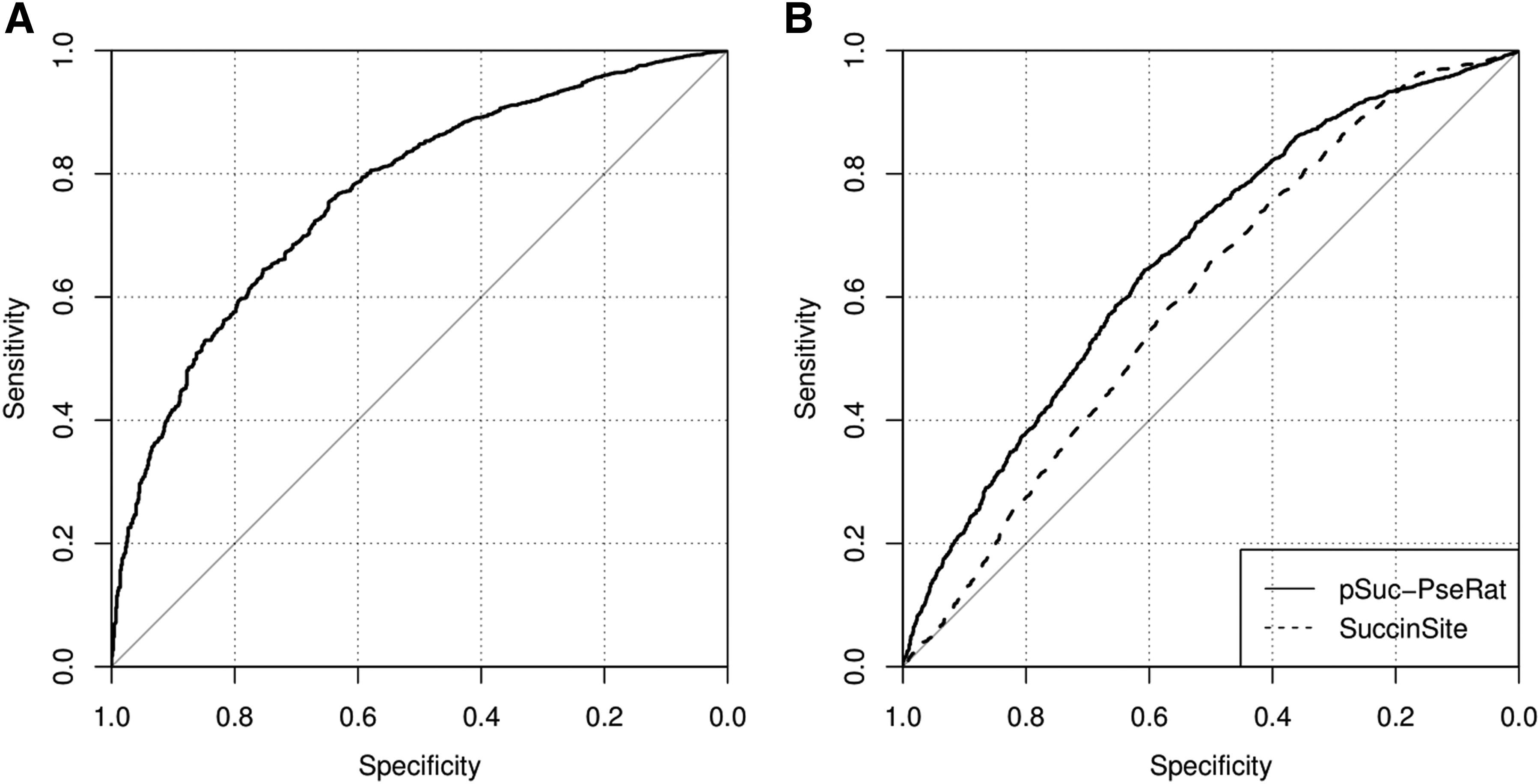(11)]; the result was named GBM ( \documentclass{aastex}\usepackage{amsbsy}\usepackage{amsfonts}\usepackage{amssymb}\usepackage{bm}\usepackage{mathrsfs}\usepackage{pifont}\usepackage{stmaryrd}\usepackage{textcomp}\usepackage{portland, xspace}\usepackage{amsmath, amsxtra}\usepackage{upgreek}\pagestyle{empty}\DeclareMathSizes{10}{9}{7}{6}\begin{document} $$\mathbb{I}$$ \end{document} ) and is listed at the bottom of Table 5. We also achieved an AUC score of 0.767, which is displayed in Figure 1A.

FIG. 1.

The performance of ROC curves. (A) Performance based on the independent test set \documentclass{aastex}\usepackage{amsbsy}\usepackage{amsfonts}\usepackage{amssymb}\usepackage{bm}\usepackage{mathrsfs}\usepackage{pifont}\usepackage{stmaryrd}\usepackage{textcomp}\usepackage{portland, xspace}\usepackage{amsmath, amsxtra}\usepackage{upgreek}\pagestyle{empty}\DeclareMathSizes{10}{9}{7}{6}\begin{document} $$\mathbb{I}$$ \end{document} in Equation (4). (B) Performance of SuccinSite and pSuc-PseRat based on the independent test \documentclass{aastex}\usepackage{amsbsy}\usepackage{amsfonts}\usepackage{amssymb}\usepackage{bm}\usepackage{mathrsfs}\usepackage{pifont}\usepackage{stmaryrd}\usepackage{textcomp}\usepackage{portland, xspace}\usepackage{amsmath, amsxtra}\usepackage{upgreek}\pagestyle{empty}\DeclareMathSizes{10}{9}{7}{6}\begin{document} $$\mathbb{I} ^\prime$$ \end{document} in Equation (6). ROC, receiver operating characteristics.

Table 4.

The Performances in Different Machine-learning Algorithms to Predict \documentclass{aastex}\usepackage{amsbsy}\usepackage{amsfonts}\usepackage{amssymb}\usepackage{bm}\usepackage{mathrsfs}\usepackage{pifont}\usepackage{stmaryrd}\usepackage{textcomp}\usepackage{portland, xspace}\usepackage{amsmath, amsxtra}\usepackage{upgreek}\pagestyle{empty}\DeclareMathSizes{10}{9}{7}{6}\begin{document} $${ \mathbb{T}_1} \ \left( {{ \rm{Eq}}. \ 10} \right)$$ \end{document}

	AUC	Sen	Spe	Acc	MCC
GBM(1)	0.800	0.737	0.714	0.726	0.458
Random Forest(1)	0.790	0.748	0.692	0.720	0.441
SVM(1)	0.785	0.743	0.693	0.718	0.436
KNN(1)	0.712	0.658	0.658	0.658	0.316
Decision Tree(1)	0.662	0.652	0.613	0.633	0.265

KNN, K-Nearest Neighbor; SVM, support vector machine.

Table 5.

The Training set [ Eq. (10) ] Performances of the GBM Classifiers with Fivefold Cross-validation, GBM(i), i = 1, 2, 3…, 11; the “i” Presents Each Number of the GBM Classifiers in the Experiment

	n.trees	AUC	Sen	Spe	Acc	MCC
GBM(1)	4400	0.800	0.737	0.714	0.726	0.458
GBM(2)	4850	0.806	0.741	0.722	0.732	0.463
GBM(3)	4500	0.803	0.743	0.717	0.730	0.461
GBM(4)	4500	0.805	0.739	0.716	0.728	0.456
GBM(5)	4300	0.806	0.741	0.721	0.731	0.462
GBM(6)	4150	0.808	0.743	0.721	0.732	0.464
GBM(7)	4900	0.806	0.740	0.730	0.735	0.471
GBM(8)	5000	0.801	0.739	0.718	0.728	0.457
GBM(9)	4650	0.807	0.738	0.723	0.731	0.462
GBM(10)	4150	0.804	0.741	0.717	0.729	0.458
GBM(11)	5000	0.809	0.742	0.722	0.732	0.464
GBM( \documentclass{aastex}\usepackage{amsbsy}\usepackage{amsfonts}\usepackage{amssymb}\usepackage{bm}\usepackage{mathrsfs}\usepackage{pifont}\usepackage{stmaryrd}\usepackage{textcomp}\usepackage{portland, xspace}\usepackage{amsmath, amsxtra}\usepackage{upgreek}\pagestyle{empty}\DeclareMathSizes{10}{9}{7}{6}\begin{document} $$\mathbb{I}$$ \end{document} )	—	0.767	0.706	0.680	0.686	0.321

3.3. Comparison of the proposed pSuc-PseRat with existing methods

To compare the performance of pSuc-PseRat with existing predictors [iSuc-PseAAC and SuccFind (Xu et al., 2015a,b)], we compiled the independent test dataset \documentclass{aastex}\usepackage{amsbsy}\usepackage{amsfonts}\usepackage{amssymb}\usepackage{bm}\usepackage{mathrsfs}\usepackage{pifont}\usepackage{stmaryrd}\usepackage{textcomp}\usepackage{portland, xspace}\usepackage{amsmath, amsxtra}\usepackage{upgreek}\pagestyle{empty}\DeclareMathSizes{10}{9}{7}{6}\begin{document} $$\mathbb{I}$$ \end{document} [Eq. (4)], which contains 704 succinylation and 2665 non-succinylation sites. Dataset \documentclass{aastex}\usepackage{amsbsy}\usepackage{amsfonts}\usepackage{amssymb}\usepackage{bm}\usepackage{mathrsfs}\usepackage{pifont}\usepackage{stmaryrd}\usepackage{textcomp}\usepackage{portland, xspace}\usepackage{amsmath, amsxtra}\usepackage{upgreek}\pagestyle{empty}\DeclareMathSizes{10}{9}{7}{6}\begin{document} $$\mathbb{I}$$ \end{document} was submitted to the existing succinylation prediction online servers, such as iSuc-PseAAC and SuccFind. The Sen, Sep, Acc, and MCC performance measurements were used to assess the prediction capability of the servers. Since the probability of non-succinylated sites is not reported in the results of the online servers, the AUC values of these servers cannot be calculated. As shown in Table 6, the Sen, Sep, and Acc for iSuc-PseAAC were 0.152, 0.868, and 0.719, respectively, and the corresponding MCC was only ∼0.024. For SuccFind, the Sen, Sep, and Acc were 0.585, 0.512, and 0.527, respectively, and the corresponding MCC was only ∼0.079. AUC and MCC are known to be more appropriate performance criteria than Acc in the evaluation of the training of classification models by the unbalanced dataset \documentclass{aastex}\usepackage{amsbsy}\usepackage{amsfonts}\usepackage{amssymb}\usepackage{bm}\usepackage{mathrsfs}\usepackage{pifont}\usepackage{stmaryrd}\usepackage{textcomp}\usepackage{portland, xspace}\usepackage{amsmath, amsxtra}\usepackage{upgreek}\pagestyle{empty}\DeclareMathSizes{10}{9}{7}{6}\begin{document} $$\mathbb{I}$$ \end{document} (Bradley, 1997; Olsson and Cotton, 1997). Clearly, the MCC value for the pSuc-PseRat predictor was significantly better than that of iSuc-PseAAC and SuccFind.

Table 6.

A Comparison of pSuc-PseRat with Existing Predictors by Using an Independent Test Set \documentclass{aastex}\usepackage{amsbsy}\usepackage{amsfonts}\usepackage{amssymb}\usepackage{bm}\usepackage{mathrsfs}\usepackage{pifont}\usepackage{stmaryrd}\usepackage{textcomp}\usepackage{portland, xspace}\usepackage{amsmath, amsxtra}\usepackage{upgreek}\pagestyle{empty}\DeclareMathSizes{10}{9}{7}{6}\begin{document} $$\mathbb{I}$$ \end{document} in Equation (4)

Predictor name	AUC	Sen	Sep	Acc	MCC
iSuc-PseAAC	—	0.152	0.868	0.719	0.024
SuccFind	—	0.585	0.512	0.527	0.079
pSuc-PseRat	0.767	0.706	0.680	0.686	0.321

The threshold values of iSuc-PseAAC and SuccFind were consistent with values defined in the servers.

To compare the performance of pSuc-PseRat with another predictor [SuccinSite (Xu et al., 2015b)], we used dataset \documentclass{aastex}\usepackage{amsbsy}\usepackage{amsfonts}\usepackage{amssymb}\usepackage{bm}\usepackage{mathrsfs}\usepackage{pifont}\usepackage{stmaryrd}\usepackage{textcomp}\usepackage{portland, xspace}\usepackage{amsmath, amsxtra}\usepackage{upgreek}\pagestyle{empty}\DeclareMathSizes{10}{9}{7}{6}\begin{document} $$\mathbb{I} ^\prime$$ \end{document} [Eq. (6)]. Here, each peptide in \documentclass{aastex}\usepackage{amsbsy}\usepackage{amsfonts}\usepackage{amssymb}\usepackage{bm}\usepackage{mathrsfs}\usepackage{pifont}\usepackage{stmaryrd}\usepackage{textcomp}\usepackage{portland, xspace}\usepackage{amsmath, amsxtra}\usepackage{upgreek}\pagestyle{empty}\DeclareMathSizes{10}{9}{7}{6}\begin{document} $$\mathbb{I} \prime$$ \end{document} was not in the datasets pSuc-PseRat or SuccinSite. Dataset \documentclass{aastex}\usepackage{amsbsy}\usepackage{amsfonts}\usepackage{amssymb}\usepackage{bm}\usepackage{mathrsfs}\usepackage{pifont}\usepackage{stmaryrd}\usepackage{textcomp}\usepackage{portland, xspace}\usepackage{amsmath, amsxtra}\usepackage{upgreek}\pagestyle{empty}\DeclareMathSizes{10}{9}{7}{6}\begin{document} $$\mathbb{I} ^\prime$$ \end{document} was submitted to the SuccinSite online server. As shown in Table 7 the Sen, Sep, and Acc values from the SuccinSite predictor were 0.304, 0.843, and 0.710, respectively, and the corresponding AUC and MCC values were 0.601 and 0.161, respectively. The AUC and MCC for pSuc-PseRat were 0.664 and 0.188, respectively. All the prediction results prove that the pSuc-PseRat predictor was better than the three predictors mentioned earlier for the prediction of succinylation sites.

Table 7.

A Comparison of pSuc-PseRat with the SuccinSite Predictors by Using the Independent Test Set \documentclass{aastex}\usepackage{amsbsy}\usepackage{amsfonts}\usepackage{amssymb}\usepackage{bm}\usepackage{mathrsfs}\usepackage{pifont}\usepackage{stmaryrd}\usepackage{textcomp}\usepackage{portland, xspace}\usepackage{amsmath, amsxtra}\usepackage{upgreek}\pagestyle{empty}\DeclareMathSizes{10}{9}{7}{6}\begin{document} $$\mathbb{I} ^\prime$$ \end{document}

Predictor name	AUC	Sen	Sep	Acc	MCC
SuccinSite	0.601	0.304	0.843	0.710	0.161
pSuc-PseRat	0.664	0.703	0.514	0.561	0.188

The threshold value of SuccinSite was selected as 0.42 from the SuccinSite server.

3.4. Web server and user guide

The web server for pSuc-PseRat has been established for convenient use by researchers, and a step-by-step guide is provided next.

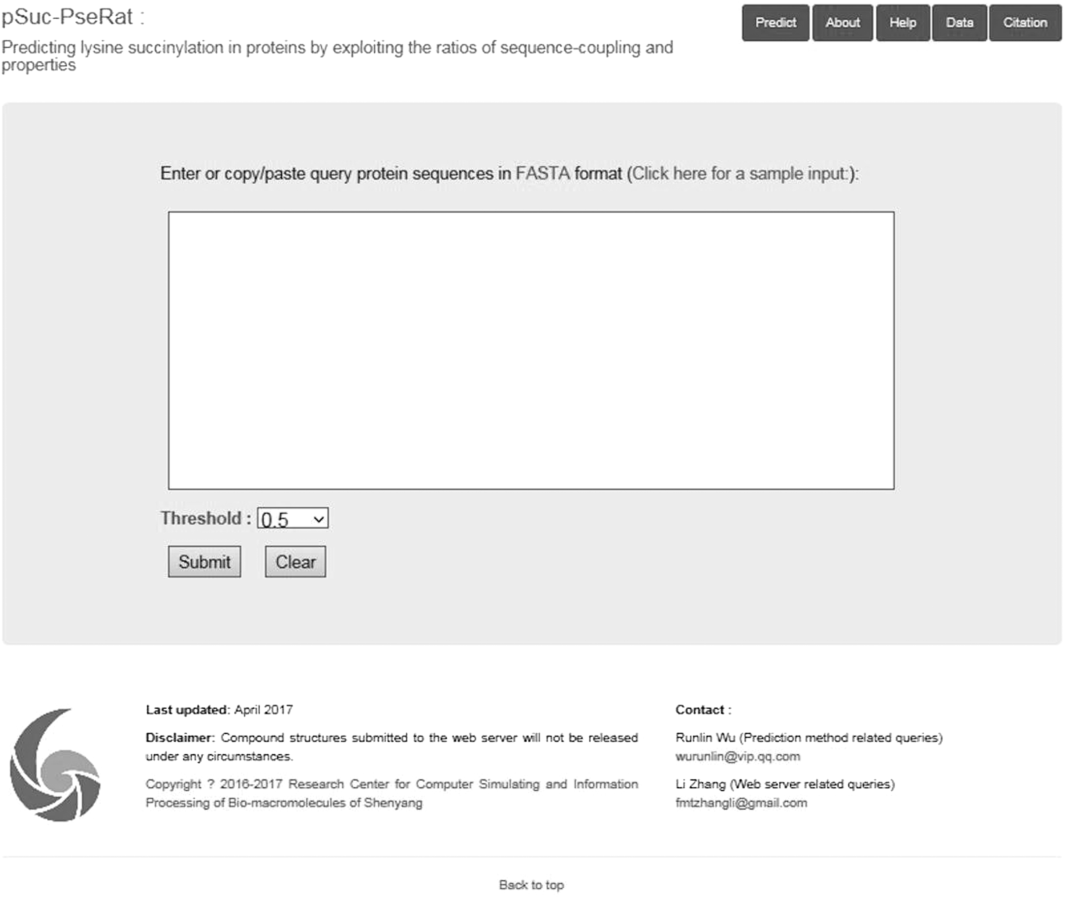
Step 1. The top page of pSuc-PseRat will be displayed by opening the web server at http://ccsipb.lnu.edu.cn/pred/succ_prediction (Fig. 2). Click on the “Documentation” button to see a brief introduction about the pSuc-PseRat predictor.

FIG. 2.

The top page of the web server of the pSuc-PseRat predictor.

Step 2. Either type or copy/paste the query protein sequences in FASTA format into the input box, as displayed in the center of Figure 2. For examples of sequences in FASTA format, click the “Click here for a sample input” button right above the input box.

Step 3. As shown in Figure 2, you may also choose to lower the threshold, which is located on the left side of the input box. If the probability score is greater than or equal to the threshold, the peptide is considered a succinylation site; otherwise, it is scored as a non-succinylation site.

Step 4. Click on the “Submit” button. The calculation and the displayed predicted results may take >40 seconds to complete, and the time required will be dependent on the total length of the protein sequences.

4. Conclusions

In this article, pSuc-PseRat was introduced as a new bioinformatics tool for predicting the succinylation sites in proteins. A new database containing 4411 experimentally verified succinylated proteins with lysine succinylation sites was used as the benchmark dataset in this study. Moreover, we solved the problem of an unbalanced dataset by Equation (5); then, we trained the GBM predictor with the PAAPP matrices [Eq. (8)] and optimized 11 randomly selected balanced training datasets to train the GBM predictor. Compared with existing predictors in this field, pSuc-PseRat achieves remarkably higher performance measurements. A web server for pSuc-PseRat has been established that can be freely accessed at http://ccsipb.lnu.edu.cn/pred/succ_prediction. We anticipate that pSuc-PseRat will be a valuable high-throughput tool that aids basic research and drug development.

Footnotes

Acknowledgments

This research was supported by the following funds: National Natural Science Foundation of China (No. 31570160), HL; Nature Science Foundation (No. 2013225086) and Science of Public Research Foundation (No. 2014001015) from the Scientific and Technological Department of Liaoning Province, H.L., H.A; Innovation Team Project (No. LT2015011) and General Research Project Foundation (No. L2014001) from the Education Department of Liaoning Province, H.L., H.A; and Large-scale Equipment Shared Services Project (No. F15165400) and Applied Basic Research Project (No. F16205151) from the Science and Technology Bureau of Shenyang, H.L., H.A. The funders had no role in the study design, data collection and analysis, decision to publish, or preparation of this article.

Author Disclosure Statement

The authors declare that no competing financial interests exist.

References

Boeckmann

, Bairoch

, Apweiler

, et al. 2003. The SWISS-PROT protein knowledgebase and its supplement TrEMBL in 2003. Nucleic Acids Res. 31, 365–370.

Bradley

A.P.

1997. The use of the area under the ROC curve in the evaluation of machine learning algorithms. Pattern Recogn. 30, 1145–1159.

Centor

R.M.

1991. Signal detectability the use of ROC curves and their analyses. Med. Decis. Making., 11, 102–106.

Chou

K.-C.

2011. Some remarks on protein attribute prediction and pseudo amino acid composition. J. Theor. Biol., 273, 236–247.

Colak

, Xie

, Zhu

A.Y.

, et al. 2013. Identification of lysine succinylation substrates and the succinylation regulatory enzyme CobB in Escherichia coli. Mol. Cell. Proteomics., 12, 3509–3520.

Friedman

J.H.

2001. Greedy function approximation: A gradient boosting machine. Ann. Stat., 9, 1189–1232.

Gribskov

, and Robinson

N.L.

1996. Use of receiver operating characteristic (ROC) analysis to evaluate sequence matching. Comput. Biol. Chem., 20, 25–33.

Hasan

M.M.

, Yang

, Zhou

, et al. 2016. SuccinSite: A computational tool for the prediction of protein succinylation sites by exploiting the amino acid patterns and properties. Mol. Biosyst., 12, 786–795.

Huang

, Niu

, Gao

, et al. 2010. CD-HIT Suite: A web server for clustering and comparing biological sequences. Bioinformatics. 26, 680–682.

10.

Hunter

, Jones

, Mitchell

, et al. 2012. InterPro in 2011: New developments in the family and domain prediction database. Nucleic Acids Res. 40, 0306–0312.

11.

James

, Witten

, and Hastie

2013. An Introduction to Statistical Learning: With Applications in R. Springer, New York.

12.

Kim

J.H.

, Lee

, Oh

, et al. 2004. Prediction of phosphorylation sites using SVMs. Bioinformatics. 20, 3179–3184.

13.

, Hu

, Wan

, et al. 2014. Systematic identification of the lysine succinylation in the protozoan parasite Toxoplasma gondii. J. Proteome Res., 13, 6087–6095.

14.

Liu

, Fang

, Liu

, et al. 2016. iMiRNA-PseDPC: MicroRNA precursor identification with a pseudo distance-pair composition approach. J. Biomol. Struct. Dyn., 34, 223–235.

15.

Liu

, Wang

, Gao

, et al. 2014. CPLM: A database of protein lysine modifications. Nucleic Acids Res. 42, D531–D536.

16.

Olsson

P.Q.

, and Cotton

W.R.

1997. Balanced and unbalanced circulations in a primitive equation simulation of a midlatitude MCC. Part II: Analysis of balance. J. Atmos Sci., 54, 479–497.

17.

Park

, Chen

, Tishkoff

D.X.

, et al. 2013. SIRT5-mediated lysine desuccinylation impacts diverse metabolic pathways. Mol. Cell., 50, 919–930.

18.

Ren

, Gao

, Jin

, et al. 2009. Systematic study of protein sumoylation: Development of a site‐specific predictor of SUMOsp 2.0. Proteomics. 9, 3409–3412.

19.

Shao

, Xu

, Tsai

S.-N.

, et al. 2009. Computational identification of protein methylation sites through bi-profile Bayes feature extraction. PLoS One. 4, e4920.

20.

Sun

, Wong

A.K.

, and Kamel

M.S.

2009. Classification of imbalanced data: A review. Int. J. Pattern Recogn., 23, 687–719.

21.

Walsh

C.T.

, Garneau‐Tsodikova

, and Gatto

G.J.

2005. Protein posttranslational modifications: The chemistry of proteome diversifications. Angew. Chem. Int. Ed., 44, 7342–7372.

22.

Weinert

B.T.

, Schölz

, Wagner

S.A.

, et al. 2013. Lysine succinylation is a frequently occurring modification in prokaryotes and eukaryotes and extensively overlaps with acetylation. Cell Rep. 4, 842–851.

23.

Wong

Y.-H.

, Lee

T.-Y.

, Liang

H.-K.

, et al. 2007. KinasePhos 2.0: A web server for identifying protein kinase-specific phosphorylation sites based on sequences and coupling patterns. Nucleic Acids Res. 35, W588–W594.

24.

Xiao

, Min

J.-L.

, Lin

W.-Z.

, et al. 2015. iDrug-Target: Predicting the interactions between drug compounds and target proteins in cellular networking via benchmark dataset optimization approach. J. Biomol. Struct. Dyn., 33, 2221–2233.

25.

Xie

, Dai

, et al. 2012. Lysine succinylation and lysine malonylation in histones. Mol. Cell. Proteomics., 11, 100–107.

26.

H.-D.

, Shi

S.-P.

, Wen

P.-P.

, et al. 2015a. SuccFind: A novel succinylation sites online prediction tool via enhanced characteristic strategy. Bioinformatics. 31, 3748–3750.

27.

, Ding

, Wu

L.-Y.

, et al. 2013. iSNO-PseAAC: Predict cysteine S-nitrosylation sites in proteins by incorporating position specific amino acid propensity into pseudo amino acid composition. PLoS One. 8, e55844.

28.

, Ding

Y.-X.

, Ding

, et al. 2015b. iSuc-PseAAC: Predicting lysine succinylation in proteins by incorporating peptide position-specific propensity. Sci. Rep., 5, 10184.

29.

Xue

, Zhou

, Fu

, et al. 2006. SUMOsp: A web server for sumoylation site prediction. Nucleic Acids Res. 34, W254–W257.

30.

Yang

, Wang

, Chen

, et al. 2015. Succinylome analysis reveals the involvement of lysine succinylation in metabolism in pathogenic Mycobacterium tuberculosis. Mol. Cell. Proteomics., 14, 796–811.

31.

Zhang

, Tan

, Xie

, et al. 2011. Identification of lysine succinylation as a new post-translational modification. Nat. Chem. Biol., 7, 58–63.

Supplementary Material

Please find the following supplemental material available below.

For Open Access articles published under a Creative Commons License, all supplemental material carries the same license as the article it is associated with.

For non-Open Access articles published, all supplemental material carries a non-exclusive license, and permission requests for re-use of supplemental material or any part of supplemental material shall be sent directly to the copyright owner as specified in the copyright notice associated with the article.

0.84 MB

0.00 MB