Phenotype Analysis Method for Identification of Gene Functions Involved in Asymmetric Division of Caenorhabditis elegans

Abstract

In gene function analysis, it is arduous to identify gene function individually, and the way to screen out all involved genes according to a particular phenotype or disease usually shows us little information for a specific problem. We present a data-driven analysis system based on wild type (WT) embryos to study the concrete function of each gene associated with certain category of abnormal phenotypes. It can be applied to genes with very few RNAi embryos. Instead of presupposing the particular function of a gene, its function is confirmed by the statistical testing of built models. The scheme includes the following five: first, verify the to be detected genes and determine related recognized features according to the given category; second, compute the value of each feature based on WT embryos and merge them by principal component analysis (PCA); third, for each of the selected components of PCA, build a normal distribution and verify its normality; fourth, project the RNAi embryos to each component and probe them; and finally, analyze the more detailed functions of each gene based on the physical or biological meaning of each component. Choosing the first-round asymmetric division process of Caenorhabditis elegans as the phenotype, experimental results show that on the different aspects of the asymmetric division process, par-2 , par-3, and let-754 are related to scalar differences; dcn-1 and mcm-5 are associated with the divergences of scalar variation, which may reflect the disaccord in development; and dcn-1 , par-2 , and par-3 are involved with morphological discrepancies.

1. Introduction

The gene function analysis in vivo phenotype is a crucial and challenging step to figure out the molecular network. There are two common ways to conduct the analysis. One way is stating an abnormal phenotype and then screening out the involved genes (Neumüller and Perrimon, 2011). For example, Ashrafi et al. (2003) experimentally screened the genes one by one and identified those genes involved in fat. Bai et al. (2008) analyzed the randomly chosen 1140 genes and found 49 genes associated with late muscle differentiation. Another way is focusing on a particular gene and identifying its functions. Fu et al. (2007) summarized wheat functional gene analysis using RNAi.

Many of the works in it were conducted by experimentally analyzing abnormal phenotypes from silencing a particular gene. Hamahashi et al. (2007) presented a system that automatically measures the cell division pattern of Caenorhabditis elegans. They also statistically analyzed two inferences on the spatial arrangement of cells and the span between the end of the four-cell stage and the beginning of the eight-cell stage of C. elegans for both par-1 mutation embryos and wild-type (WT) embryos. However, the former way only provides faint information for identifying concrete gene functions, and the latter method is not only arduous but also restrained. The first limitation of it is that we usually need a large number of RNAi and WT embryos to reach a statistical result. The second limitation lies in the efficiency. To verify whether a certain gene has a presupposed function or not, the common method is selecting features according to the function and statistically testing the WT and RNAi embryos, which is problem oriented and only applicable for a predetermined problem related to a particular gene function. Therefore, its efficiency is limited in large-scale gene analysis.

In this article, we propose a WT-based data-driven method to study the concrete function of each gene associated with a specific category of abnormal phenotypes. It firstly determines the recognized features based on a certain phenotype and all the involved genes. Then, after merging these features using principal component analysis (PCA), statistical models are built based on a large number of WT embryos. Finally, different RNAi embryos corresponding to all the involved genes are screened with the built statistical models. The advantages of this approach are as follows: first, it can be applied to genes with a small number of RNAi embryos; second, a number of genes can be analyzed using the same models; and third, it is not necessary to presuppose the particular function of a gene, instead its function is confirmed by the statistical testing results of the built models. To evaluate the effectiveness of the framework, we choose the phenotype, P₁/AB asynchrony of divisions, as an example.

The nematode C. elegans is one of few animals in which essential embryonic genes have been identified through genomewide RNAi screening (Fraser et al., 2000). It also has a fixed cell lineage and a precise cell fate map (Sulston et al., 1983), which makes it a perfect animal to functional gene analysis.

Cell division of C. elegans is asymmetric, generating the two daughter cells with different sizes, which plays an important role in the generation of cellular diversity during development (Horvitz and Herskowitz, 1992; Guo and Kemphues, 1995). The asymmetry of division is crucial not only to C. elegans but also to Drosophila melanogaster and mouse (Betschinger and Knoblich, 2004; Gönczy, 2008).

Usually, for the first two blastomeres of a WT embryo, the anterior blastomere (AB) is arguably larger than the posterior blastomere (P₁) (Arata et al., 2015). Kemphues et al. (1988) verified that silencing par-1, par-2, and par-3 might disturb the normally asymmetric cleavage and generate variant daughter cells. More relevant analysis can also be seen in Hara et al. (2013) and Ladouceur et al. (2015). In Phenobank (Sönnichsen et al., 2005), currently known genes with the similar function that may influence the first round of cell division (from P₀ to P₁ and AB) are compiled in the category of “P₁/AB Asynchrony of Divisions.” Although these genes have been found and listed in Phenobank, their, respectively, specific functions on the first round of cellular division remain unclear. The asynchrony of division may express in multiple facets, such as the difference of lifetime, size, growth ratio, or geometric shape. Understanding the specific function of these genes is valuable to finally comprehend the whole gene expression regulatory network. Because the proposed method requires a large number of WT embryos to carry out the analysis, we use Worm Developmental Dynamics Database (WDDD) as the database. WDDD includes the records of 136 RNAi and 50 WT embryos developing from 1 to 16 cells (Kyoda et al., 2013), which makes it a desired platform (see Section 3.1. for details) for our study.

2. Methods

2.1. Data

Using four-dimensional (4D) differential interference contrast (DIC) microscopy, WDDD has 50 sets of quantitative data from WT embryos. After silencing embryonic genes on chromosome III individually, 72 genes with 136 sets of quantitative data from RNAi experiments were also built (Kyoda et al., 2013; http://so.qbic.riken.jp/wddd). For each set, there are 180 time points (40 seconds/time point), and a three-dimensional (3D) image is stored at each time point. In each 3D image, the z-stack includes 66 focal planes (0.5 μm/plane) and there are 600 × 600 pixels (0.105 μm/pixel) in each focal plane. Besides 4D DIC images, WDDD also provides the dynamic coordinates of outlines of each nuclear region during the first three rounds of division and their corresponding blastomere names. In the 72 genes, 6 of them are categorized into “P₁/AB Asynchrony of Divisions” in the Phenobank. They are dcn-1, ket-754, mcm-5, par-2, par-3, and rnr-1.

After checking the number of time points of P₁ and AB for the 136 embryos, we discard deficient embryos for two reasons as follows: (1) the P₁ or AB dies (without daughters) and (2) the number of time points of P₁ (or AB) is less than 3 (therefore, the computed features may be unreliable.) Among the discarded embryos, T23G5.1_061102_01 belongs to rnr-1. Thus, we use the remains of five genes. Its corresponding RNAi embryos are shown in Table 1.

Table 1.

To Be Detected Genes and RNAi Embryos In Worm Developmental Dynamics Database

Gene	dcn-1	let-754	mcm-5	par-2	par-3
Embryo1	H38K22.2_040810_01	C29E4.8_040610_01	R10E4.4_061107_01	F58B6.3_080401_01	F54E7.3_070927_01
Embryo2	H38K22.2_040810_02	C29E4.8_040610_02	R10E4.4_061107_02	F58B6.3_080610_02	F54E7.3_071121_01

2.2. The Algorithm

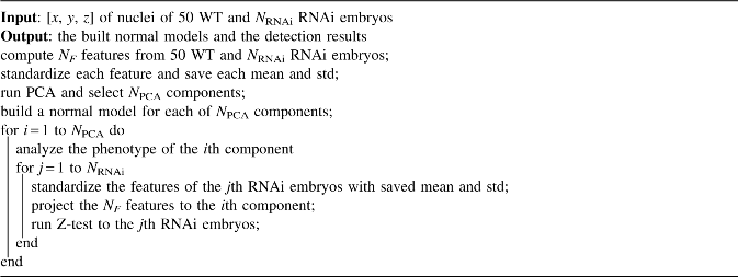
According to the introduction, we can build the Algorithm 1 (N_RNAi is the number of RNAi embryos, here is 10; N_F is the number of features, here is 10; and N_PCA is the number of chosen components, here is 4). In Sections 2.3.–2.6., we will interpret each step of the algorithm.

Algorithm 1.

The algorithm of gene function analysis

2.3. Features

2.3.1. Choosing features

A nucleus of P₁ is arguably smaller and more slender than AB. Therefore, we use four well-known features: volume, surface, diameter, and compactness to measure. The first three characteristics are related to size, whereas the last one reflects the level of slenderness. Although there are many shape characteristics being proposed (Loncaric, 1998; Zhang and Lu, 2004), the four characteristics used in this study are both easy to compute and well recognized. For each embryo, there are many time points (usually 15–40) and corresponding nuclei at the stage of P₁ (or AB). For the purpose of condensing data, we use mean value and standard deviation (std) in the period of P₁ (or AB) to reflect the morphological characteristics.

The definition of diameter in 3D space used in this article is a natural generalization of the definition in two-dimensional (2D) space. We call the distance between two parallel tangent planes of an object as diameter. It is also known as Feret diameters (Glasbey and Horgan, 1995). Along one direction in 3D space we can calculate one diameter (Fig. 1). Therefore, if we choose 1000 directions in 3D space, 1000 diameters will be worked out. For a nucleus at certain time point, we can compute only one value for volume or surface, whereas for diameter, the number of computed values is 1000 if we use 1000 directions. Based on these values, we compute the mean value to reflect their size and the ratio of the minimal value to the maximal value (min/max) to reflect their compactness. After that, we can calculate the mean value and std value for an embryo on the whole time points within the period of P₁ (or AB). In summary, we use 10 features (Table 2) to analyze.

FIG. 1.

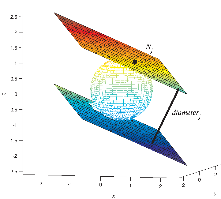
Feret diameter. x, y, and z are the three orthogonal axes in euclidean space.

Table 2.

List of 10 Features

Nth	Feature	Nth	Feature
1	Volume mean	6	Diameter mean std
2	Volume std	7	Diameter min/max mean
3	Surface mean	8	Diameter min/max std
4	Surface std	9	Compactness mean
5	Diameter mean	10	Compactness std

2.3.2. The computation of the features

WDDD provides the coordinates of outlines for each nuclear region. To simplify the computation, we use the number of involved voxels to represent volume and surface area. Rosenfeld pointed out that using this method to compute some classic shape characteristics such as perimeter may cause inconsistent results and give theoretical analysis (Rosenfeld, 1974). For the data in WDDD, however, because the images are built in the same way under the same condition, if we process the data of different embryos in the same way, the influence of discretization is small and will not bring meaningful errors.

2.3.2.1. Volume

For the nucleus at t (t = 1, \documentclass{aastex}\usepackage{amsbsy}\usepackage{amsfonts}\usepackage{amssymb}\usepackage{bm}\usepackage{mathrsfs}\usepackage{pifont}\usepackage{stmaryrd}\usepackage{textcomp}\usepackage{portland, xspace}\usepackage{amsmath, amsxtra}\usepackage{upgreek}\pagestyle{empty}\DeclareMathSizes{10}{9}{7}{6}\begin{document} $$\ldots,$$ \end{document} T) time point of an AB, based on the number of voxels \documentclass{aastex}\usepackage{amsbsy}\usepackage{amsfonts}\usepackage{amssymb}\usepackage{bm}\usepackage{mathrsfs}\usepackage{pifont}\usepackage{stmaryrd}\usepackage{textcomp}\usepackage{portland, xspace}\usepackage{amsmath, amsxtra}\usepackage{upgreek}\pagestyle{empty}\DeclareMathSizes{10}{9}{7}{6}\begin{document} $$V_t^{AB}$$ \end{document} within its outline, we can compute \documentclass{aastex}\usepackage{amsbsy}\usepackage{amsfonts}\usepackage{amssymb}\usepackage{bm}\usepackage{mathrsfs}\usepackage{pifont}\usepackage{stmaryrd}\usepackage{textcomp}\usepackage{portland, xspace}\usepackage{amsmath, amsxtra}\usepackage{upgreek}\pagestyle{empty}\DeclareMathSizes{10}{9}{7}{6}\begin{document} $$V_{{ \rm{mean}}}^{AB}$$ \end{document} and \documentclass{aastex}\usepackage{amsbsy}\usepackage{amsfonts}\usepackage{amssymb}\usepackage{bm}\usepackage{mathrsfs}\usepackage{pifont}\usepackage{stmaryrd}\usepackage{textcomp}\usepackage{portland, xspace}\usepackage{amsmath, amsxtra}\usepackage{upgreek}\pagestyle{empty}\DeclareMathSizes{10}{9}{7}{6}\begin{document} $$V_{{ \rm{std}}}^{AB}$$ \end{document} . After working out the features of the AB, the two features of a P₁, \documentclass{aastex}\usepackage{amsbsy}\usepackage{amsfonts}\usepackage{amssymb}\usepackage{bm}\usepackage{mathrsfs}\usepackage{pifont}\usepackage{stmaryrd}\usepackage{textcomp}\usepackage{portland, xspace}\usepackage{amsmath, amsxtra}\usepackage{upgreek}\pagestyle{empty}\DeclareMathSizes{10}{9}{7}{6}\begin{document} $$V_{{ \rm{mean}}}^{P1}$$ \end{document} and \documentclass{aastex}\usepackage{amsbsy}\usepackage{amsfonts}\usepackage{amssymb}\usepackage{bm}\usepackage{mathrsfs}\usepackage{pifont}\usepackage{stmaryrd}\usepackage{textcomp}\usepackage{portland, xspace}\usepackage{amsmath, amsxtra}\usepackage{upgreek}\pagestyle{empty}\DeclareMathSizes{10}{9}{7}{6}\begin{document} $$V_{{ \rm{std}}}^{P1}$$ \end{document} can be calculated in the same way.

2.3.2.2. Surface area

For the nucleus at t (t = 1, \documentclass{aastex}\usepackage{amsbsy}\usepackage{amsfonts}\usepackage{amssymb}\usepackage{bm}\usepackage{mathrsfs}\usepackage{pifont}\usepackage{stmaryrd}\usepackage{textcomp}\usepackage{portland, xspace}\usepackage{amsmath, amsxtra}\usepackage{upgreek}\pagestyle{empty}\DeclareMathSizes{10}{9}{7}{6}\begin{document} $$\ldots,$$ \end{document} T) time point of an AB, we can also count the number of voxels on the outline as \documentclass{aastex}\usepackage{amsbsy}\usepackage{amsfonts}\usepackage{amssymb}\usepackage{bm}\usepackage{mathrsfs}\usepackage{pifont}\usepackage{stmaryrd}\usepackage{textcomp}\usepackage{portland, xspace}\usepackage{amsmath, amsxtra}\usepackage{upgreek}\pagestyle{empty}\DeclareMathSizes{10}{9}{7}{6}\begin{document} $$S_t^{AB}$$ \end{document} . Based on \documentclass{aastex}\usepackage{amsbsy}\usepackage{amsfonts}\usepackage{amssymb}\usepackage{bm}\usepackage{mathrsfs}\usepackage{pifont}\usepackage{stmaryrd}\usepackage{textcomp}\usepackage{portland, xspace}\usepackage{amsmath, amsxtra}\usepackage{upgreek}\pagestyle{empty}\DeclareMathSizes{10}{9}{7}{6}\begin{document} $$S_t^{AB}$$ \end{document} , we can compute the two features \documentclass{aastex}\usepackage{amsbsy}\usepackage{amsfonts}\usepackage{amssymb}\usepackage{bm}\usepackage{mathrsfs}\usepackage{pifont}\usepackage{stmaryrd}\usepackage{textcomp}\usepackage{portland, xspace}\usepackage{amsmath, amsxtra}\usepackage{upgreek}\pagestyle{empty}\DeclareMathSizes{10}{9}{7}{6}\begin{document} $$S_{{ \rm{mean}}}^{AB}$$ \end{document} and \documentclass{aastex}\usepackage{amsbsy}\usepackage{amsfonts}\usepackage{amssymb}\usepackage{bm}\usepackage{mathrsfs}\usepackage{pifont}\usepackage{stmaryrd}\usepackage{textcomp}\usepackage{portland, xspace}\usepackage{amsmath, amsxtra}\usepackage{upgreek}\pagestyle{empty}\DeclareMathSizes{10}{9}{7}{6}\begin{document} $$S_{{ \rm{std}}}^{AB}$$ \end{document} , and \documentclass{aastex}\usepackage{amsbsy}\usepackage{amsfonts}\usepackage{amssymb}\usepackage{bm}\usepackage{mathrsfs}\usepackage{pifont}\usepackage{stmaryrd}\usepackage{textcomp}\usepackage{portland, xspace}\usepackage{amsmath, amsxtra}\usepackage{upgreek}\pagestyle{empty}\DeclareMathSizes{10}{9}{7}{6}\begin{document} $$S_{{ \rm{mean}}}^{P1}$$ \end{document} and \documentclass{aastex}\usepackage{amsbsy}\usepackage{amsfonts}\usepackage{amssymb}\usepackage{bm}\usepackage{mathrsfs}\usepackage{pifont}\usepackage{stmaryrd}\usepackage{textcomp}\usepackage{portland, xspace}\usepackage{amsmath, amsxtra}\usepackage{upgreek}\pagestyle{empty}\DeclareMathSizes{10}{9}{7}{6}\begin{document} $$S_{{ \rm{std}}}^{P1}$$ \end{document} can be obtained similarly.

2.3.2.3. Diameter

According to the meaning of diameter in this article, we use Golden Section Spiral (GSS) method (Treeby and Cox, 2010) to obtain evenly scattered N_d points \documentclass{aastex}\usepackage{amsbsy}\usepackage{amsfonts}\usepackage{amssymb}\usepackage{bm}\usepackage{mathrsfs}\usepackage{pifont}\usepackage{stmaryrd}\usepackage{textcomp}\usepackage{portland, xspace}\usepackage{amsmath, amsxtra}\usepackage{upgreek}\pagestyle{empty}\DeclareMathSizes{10}{9}{7}{6}\begin{document} $${Q_d} = [ e_d^1 , e_d^2 , e_d^3 ]$$ \end{document} (d = 1,…, N_d) in a unit sphere to represent N_d directions (the direction is along its normal vector for a point in the surface of the unit sphere). Figure 2 shows the generated points by GSS in a half unit sphere. We can derive the relationship: \documentclass{aastex}\usepackage{amsbsy}\usepackage{amsfonts}\usepackage{amssymb}\usepackage{bm}\usepackage{mathrsfs}\usepackage{pifont}\usepackage{stmaryrd}\usepackage{textcomp}\usepackage{portland, xspace}\usepackage{amsmath, amsxtra}\usepackage{upgreek}\pagestyle{empty}\DeclareMathSizes{10}{9}{7}{6}\begin{document} \begin{align*} { \theta _ { { \rm { space } } } } = \frac { { 180 } } { \pi } \cdot \arccos ( 1 - { \frac { 8 \pi } { \sqrt 3 \cdot { N_d } } } ) , \tag { 1 } \end{align*} \end{document}

between N_d and the central angle θ_space of two adjacent points Q_d, Q_d₊₁ (Fig. 3)_. The computation burden and the computation accuracy are a trade-off. In this study, we set N_d = 1000, which makes the θ_space less than 10°.

FIG. 2.

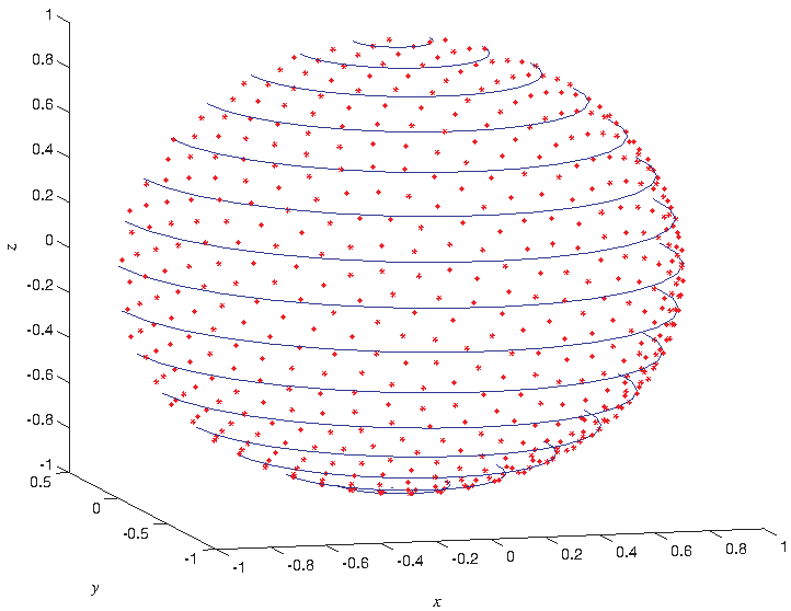
The generated points in a half sphere by GSS; x, y, and z are three orthogonal axes in euclidean space. GSS, golden section spiral.

FIG. 3.

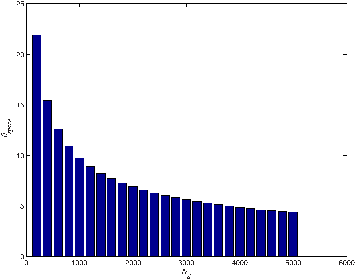
The relationship between N_d and the angle interval. x-axis represents N_d, and y-axis is the angle interval.

We use two steps to calculate the features related to diameter. (1) The computation of diameter. For the nucleus at t (t = 1,…,T) time point of an AB, using: \documentclass{aastex}\usepackage{amsbsy}\usepackage{amsfonts}\usepackage{amssymb}\usepackage{bm}\usepackage{mathrsfs}\usepackage{pifont}\usepackage{stmaryrd}\usepackage{textcomp}\usepackage{portland, xspace}\usepackage{amsmath, amsxtra}\usepackage{upgreek}\pagestyle{empty}\DeclareMathSizes{10}{9}{7}{6}\begin{document} \begin{align*} D_d^t = \max ( \rho _{d , v}^t \vert v = 1 , \ldots , {N_v} ) - \min ( \rho _{d , v}^t \vert v = 1 , \ldots , {N_v} ). \tag{2} \end{align*} \end{document} \documentclass{aastex}\usepackage{amsbsy}\usepackage{amsfonts}\usepackage{amssymb}\usepackage{bm}\usepackage{mathrsfs}\usepackage{pifont}\usepackage{stmaryrd}\usepackage{textcomp}\usepackage{portland, xspace}\usepackage{amsmath, amsxtra}\usepackage{upgreek}\pagestyle{empty}\DeclareMathSizes{10}{9}{7}{6}\begin{document} \begin{align*} \rho _{d , v}^t = P_v^t \cdot {Q_d} = 1.05x_v^te_d^1 + 1.05y_v^te_d^2 + 5z_v^te_d^3 , \ \mathop \sum \limits_{i = 1}^3 {{{ ( e_d^i ) }^2}} = 1 , \ d = 1 , \ldots , {N_d}. \tag{3} \end{align*} \end{document}

(2) Compute the features related to diameter. The equations are: \documentclass{aastex}\usepackage{amsbsy}\usepackage{amsfonts}\usepackage{amssymb}\usepackage{bm}\usepackage{mathrsfs}\usepackage{pifont}\usepackage{stmaryrd}\usepackage{textcomp}\usepackage{portland, xspace}\usepackage{amsmath, amsxtra}\usepackage{upgreek}\pagestyle{empty}\DeclareMathSizes{10}{9}{7}{6}\begin{document} \begin{align*} D_ { { \rm { mean , mean } } } ^ { AB } = \frac { 1 } { T } \mathop \sum \limits_ { t = 1 } ^T { D_ { { \rm { mean } } } ^t } , D_ { { \rm { min / max , mean } } } ^ { AB } = \frac { 1 } { T } \mathop \sum \limits_ { t = 1 } ^T { { \frac { D_ { \min } ^t } { D_ { \max } ^t } } } ,\tag { 4 } \end{align*} \end{document} \documentclass{aastex}\usepackage{amsbsy}\usepackage{amsfonts}\usepackage{amssymb}\usepackage{bm}\usepackage{mathrsfs}\usepackage{pifont}\usepackage{stmaryrd}\usepackage{textcomp}\usepackage{portland, xspace}\usepackage{amsmath, amsxtra}\usepackage{upgreek}\pagestyle{empty}\DeclareMathSizes{10}{9}{7}{6}\begin{document} \begin{align*} D_ { { \rm { mean , std } } } ^ { AB } = \sqrt { \frac { 1 } { { T - 1 } } \mathop \sum \limits_ { t = 1 } ^T { { { ( D_ { { \rm { mean } } } ^t - D_ { { \rm { mean , mean } } } ^ { AB } ) } ^2 } } } , \tag { 5 } \end{align*} \end{document} \documentclass{aastex}\usepackage{amsbsy}\usepackage{amsfonts}\usepackage{amssymb}\usepackage{bm}\usepackage{mathrsfs}\usepackage{pifont}\usepackage{stmaryrd}\usepackage{textcomp}\usepackage{portland, xspace}\usepackage{amsmath, amsxtra}\usepackage{upgreek}\pagestyle{empty}\DeclareMathSizes{10}{9}{7}{6}\begin{document} \begin{align*} D_ { { \rm { min / max , std } } } ^ { AB } = \sqrt { \frac { 1 } { { T - 1 } } \mathop \sum \limits_ { t = 1 } ^T { { { ( { \frac { D_ { \min } ^t } { D_ { \max } ^t } } - D_ { { \rm { min / max , mean } } } ^ { AB } ) } ^2 } } } . \tag { 6 } \end{align*} \end{document} \documentclass{aastex}\usepackage{amsbsy}\usepackage{amsfonts}\usepackage{amssymb}\usepackage{bm}\usepackage{mathrsfs}\usepackage{pifont}\usepackage{stmaryrd}\usepackage{textcomp}\usepackage{portland, xspace}\usepackage{amsmath, amsxtra}\usepackage{upgreek}\pagestyle{empty}\DeclareMathSizes{10}{9}{7}{6}\begin{document} \begin{align*} D_ { { \rm { mean } } } ^t = \frac { 1 } { { { N_d } } } \mathop \sum \limits_ { d = 1 } ^ { { N_d } } { D_d^t } , D_ { \max } ^t = \max ( D_d^t \vert d = 1 , \ldots , { N_d } ) , D_ { \min } ^t = \min ( D_d^t \vert d = 1 , \ldots , { N_d } ). \end{align*} \end{document}

Then, we can compute \documentclass{aastex}\usepackage{amsbsy}\usepackage{amsfonts}\usepackage{amssymb}\usepackage{bm}\usepackage{mathrsfs}\usepackage{pifont}\usepackage{stmaryrd}\usepackage{textcomp}\usepackage{portland, xspace}\usepackage{amsmath, amsxtra}\usepackage{upgreek}\pagestyle{empty}\DeclareMathSizes{10}{9}{7}{6}\begin{document} $$D_{{ \rm{mean , mean}}}^{P1}$$ \end{document} , \documentclass{aastex}\usepackage{amsbsy}\usepackage{amsfonts}\usepackage{amssymb}\usepackage{bm}\usepackage{mathrsfs}\usepackage{pifont}\usepackage{stmaryrd}\usepackage{textcomp}\usepackage{portland, xspace}\usepackage{amsmath, amsxtra}\usepackage{upgreek}\pagestyle{empty}\DeclareMathSizes{10}{9}{7}{6}\begin{document} $$D_{{ \rm{mean , std}}}^{P1}$$ \end{document} , \documentclass{aastex}\usepackage{amsbsy}\usepackage{amsfonts}\usepackage{amssymb}\usepackage{bm}\usepackage{mathrsfs}\usepackage{pifont}\usepackage{stmaryrd}\usepackage{textcomp}\usepackage{portland, xspace}\usepackage{amsmath, amsxtra}\usepackage{upgreek}\pagestyle{empty}\DeclareMathSizes{10}{9}{7}{6}\begin{document} $$D_{{ \rm{min / max , mean}}}^{P1}$$ \end{document} , and \documentclass{aastex}\usepackage{amsbsy}\usepackage{amsfonts}\usepackage{amssymb}\usepackage{bm}\usepackage{mathrsfs}\usepackage{pifont}\usepackage{stmaryrd}\usepackage{textcomp}\usepackage{portland, xspace}\usepackage{amsmath, amsxtra}\usepackage{upgreek}\pagestyle{empty}\DeclareMathSizes{10}{9}{7}{6}\begin{document} $$D_{{ \rm{min / max , std}}}^{P1}$$ \end{document} similarly.

2.3.2.4. Compactness

The computation of compactness (Attneave and Arnoult, 1956) is based on Young et al. (1974). For the nucleus at t (t = 1,…,T) time point of an AB, based on the computed V_t^AB and S_t^AB, we can derive: \documentclass{aastex}\usepackage{amsbsy}\usepackage{amsfonts}\usepackage{amssymb}\usepackage{bm}\usepackage{mathrsfs}\usepackage{pifont}\usepackage{stmaryrd}\usepackage{textcomp}\usepackage{portland, xspace}\usepackage{amsmath, amsxtra}\usepackage{upgreek}\pagestyle{empty}\DeclareMathSizes{10}{9}{7}{6}\begin{document} \begin{align*} C_t^ { AB } = \frac { 1 } { { 36 \pi } } { \frac { { { ( S_t^ { AB } ) } ^3 } } { { { ( V_t^ { AB } ) } ^2 } } } , t = 1 , \ldots , T. \tag { 7 } \end{align*} \end{document}

The two features \documentclass{aastex}\usepackage{amsbsy}\usepackage{amsfonts}\usepackage{amssymb}\usepackage{bm}\usepackage{mathrsfs}\usepackage{pifont}\usepackage{stmaryrd}\usepackage{textcomp}\usepackage{portland, xspace}\usepackage{amsmath, amsxtra}\usepackage{upgreek}\pagestyle{empty}\DeclareMathSizes{10}{9}{7}{6}\begin{document} $$C_{{ \rm{mean}}}^{AB}$$ \end{document} and \documentclass{aastex}\usepackage{amsbsy}\usepackage{amsfonts}\usepackage{amssymb}\usepackage{bm}\usepackage{mathrsfs}\usepackage{pifont}\usepackage{stmaryrd}\usepackage{textcomp}\usepackage{portland, xspace}\usepackage{amsmath, amsxtra}\usepackage{upgreek}\pagestyle{empty}\DeclareMathSizes{10}{9}{7}{6}\begin{document} $$C_{{ \rm{std}}}^{AB}$$ \end{document} related to compactness can be computed accordingly. Similarly, we can compute \documentclass{aastex}\usepackage{amsbsy}\usepackage{amsfonts}\usepackage{amssymb}\usepackage{bm}\usepackage{mathrsfs}\usepackage{pifont}\usepackage{stmaryrd}\usepackage{textcomp}\usepackage{portland, xspace}\usepackage{amsmath, amsxtra}\usepackage{upgreek}\pagestyle{empty}\DeclareMathSizes{10}{9}{7}{6}\begin{document} $$C_{{ \rm{mean}}}^{P1}$$ \end{document} and \documentclass{aastex}\usepackage{amsbsy}\usepackage{amsfonts}\usepackage{amssymb}\usepackage{bm}\usepackage{mathrsfs}\usepackage{pifont}\usepackage{stmaryrd}\usepackage{textcomp}\usepackage{portland, xspace}\usepackage{amsmath, amsxtra}\usepackage{upgreek}\pagestyle{empty}\DeclareMathSizes{10}{9}{7}{6}\begin{document} $$C_{{ \rm{std}}}^{P1}$$ \end{document} .

2.3.3. The final built features

2.3.3.1. Normalizing magnitude

After computing the features related to volume, surface, diameter, and compactness, we adjust their magnitudes to keep them in line with the length. After standardizing, the final used features are (the features of AB are similar): \documentclass{aastex}\usepackage{amsbsy}\usepackage{amsfonts}\usepackage{amssymb}\usepackage{bm}\usepackage{mathrsfs}\usepackage{pifont}\usepackage{stmaryrd}\usepackage{textcomp}\usepackage{portland, xspace}\usepackage{amsmath, amsxtra}\usepackage{upgreek}\pagestyle{empty}\DeclareMathSizes{10}{9}{7}{6}\begin{document} $$F_1^{P1} = \root 3 \of {V_{{ \rm{mean}}}^{P1}}$$ \end{document} , \documentclass{aastex}\usepackage{amsbsy}\usepackage{amsfonts}\usepackage{amssymb}\usepackage{bm}\usepackage{mathrsfs}\usepackage{pifont}\usepackage{stmaryrd}\usepackage{textcomp}\usepackage{portland, xspace}\usepackage{amsmath, amsxtra}\usepackage{upgreek}\pagestyle{empty}\DeclareMathSizes{10}{9}{7}{6}\begin{document} $$F_2^{P1} = \root 3 \of {V_{{ \rm{std}}}^{P1}}$$ \end{document} , \documentclass{aastex}\usepackage{amsbsy}\usepackage{amsfonts}\usepackage{amssymb}\usepackage{bm}\usepackage{mathrsfs}\usepackage{pifont}\usepackage{stmaryrd}\usepackage{textcomp}\usepackage{portland, xspace}\usepackage{amsmath, amsxtra}\usepackage{upgreek}\pagestyle{empty}\DeclareMathSizes{10}{9}{7}{6}\begin{document} $$F_3^{P1} = \sqrt {S_{{ \rm{mean}}}^{P1}}$$ \end{document} , \documentclass{aastex}\usepackage{amsbsy}\usepackage{amsfonts}\usepackage{amssymb}\usepackage{bm}\usepackage{mathrsfs}\usepackage{pifont}\usepackage{stmaryrd}\usepackage{textcomp}\usepackage{portland, xspace}\usepackage{amsmath, amsxtra}\usepackage{upgreek}\pagestyle{empty}\DeclareMathSizes{10}{9}{7}{6}\begin{document} $$F_4^{P1} = \sqrt {S_{{ \rm{std}}}^{P1}}$$ \end{document} , \documentclass{aastex}\usepackage{amsbsy}\usepackage{amsfonts}\usepackage{amssymb}\usepackage{bm}\usepackage{mathrsfs}\usepackage{pifont}\usepackage{stmaryrd}\usepackage{textcomp}\usepackage{portland, xspace}\usepackage{amsmath, amsxtra}\usepackage{upgreek}\pagestyle{empty}\DeclareMathSizes{10}{9}{7}{6}\begin{document} $$F_5^{P1} = D_{{ \rm{mean , mean}}}^{P1}$$ \end{document} , \documentclass{aastex}\usepackage{amsbsy}\usepackage{amsfonts}\usepackage{amssymb}\usepackage{bm}\usepackage{mathrsfs}\usepackage{pifont}\usepackage{stmaryrd}\usepackage{textcomp}\usepackage{portland, xspace}\usepackage{amsmath, amsxtra}\usepackage{upgreek}\pagestyle{empty}\DeclareMathSizes{10}{9}{7}{6}\begin{document} $$F_6^{P1} = D_{{ \rm{mean , std}}}^{P1}$$ \end{document} , \documentclass{aastex}\usepackage{amsbsy}\usepackage{amsfonts}\usepackage{amssymb}\usepackage{bm}\usepackage{mathrsfs}\usepackage{pifont}\usepackage{stmaryrd}\usepackage{textcomp}\usepackage{portland, xspace}\usepackage{amsmath, amsxtra}\usepackage{upgreek}\pagestyle{empty}\DeclareMathSizes{10}{9}{7}{6}\begin{document} $$F_7^{P1} = D_{{ \rm{min / max , mean}}}^{P1}$$ \end{document} , \documentclass{aastex}\usepackage{amsbsy}\usepackage{amsfonts}\usepackage{amssymb}\usepackage{bm}\usepackage{mathrsfs}\usepackage{pifont}\usepackage{stmaryrd}\usepackage{textcomp}\usepackage{portland, xspace}\usepackage{amsmath, amsxtra}\usepackage{upgreek}\pagestyle{empty}\DeclareMathSizes{10}{9}{7}{6}\begin{document} $$F_8^{P1} = D_{{ \rm{min / max , std}}}^{P1}$$ \end{document} , \documentclass{aastex}\usepackage{amsbsy}\usepackage{amsfonts}\usepackage{amssymb}\usepackage{bm}\usepackage{mathrsfs}\usepackage{pifont}\usepackage{stmaryrd}\usepackage{textcomp}\usepackage{portland, xspace}\usepackage{amsmath, amsxtra}\usepackage{upgreek}\pagestyle{empty}\DeclareMathSizes{10}{9}{7}{6}\begin{document} $$F_9^{P1} = \root 6 \of {C_{{ \rm{mean}}}^{P1}}$$ \end{document} , and \documentclass{aastex}\usepackage{amsbsy}\usepackage{amsfonts}\usepackage{amssymb}\usepackage{bm}\usepackage{mathrsfs}\usepackage{pifont}\usepackage{stmaryrd}\usepackage{textcomp}\usepackage{portland, xspace}\usepackage{amsmath, amsxtra}\usepackage{upgreek}\pagestyle{empty}\DeclareMathSizes{10}{9}{7}{6}\begin{document} $$F_{10}^{P1} = \root 6 \of {C_{{ \rm{std}}}^{P1}}$$ \end{document} .

2.3.3.2. Building features

The standardized data have removed the influence of magnitude. However, there are two values (belongs to P₁ and AB, respectively) corresponding to the identical feature of the same embryo, which is hard to handle when testing or evaluating an embryo. Therefore, suppose the 50 values of F_i^P¹ (i = 1,…,N_F, N_F = 10) are \documentclass{aastex}\usepackage{amsbsy}\usepackage{amsfonts}\usepackage{amssymb}\usepackage{bm}\usepackage{mathrsfs}\usepackage{pifont}\usepackage{stmaryrd}\usepackage{textcomp}\usepackage{portland, xspace}\usepackage{amsmath, amsxtra}\usepackage{upgreek}\pagestyle{empty}\DeclareMathSizes{10}{9}{7}{6}\begin{document} $$F_{i , j}^{P1}$$ \end{document} (j = 1,…,N_WT, N_WT = 50), for each \documentclass{aastex}\usepackage{amsbsy}\usepackage{amsfonts}\usepackage{amssymb}\usepackage{bm}\usepackage{mathrsfs}\usepackage{pifont}\usepackage{stmaryrd}\usepackage{textcomp}\usepackage{portland, xspace}\usepackage{amsmath, amsxtra}\usepackage{upgreek}\pagestyle{empty}\DeclareMathSizes{10}{9}{7}{6}\begin{document} $$F_{i , j}^{P1}$$ \end{document} and \documentclass{aastex}\usepackage{amsbsy}\usepackage{amsfonts}\usepackage{amssymb}\usepackage{bm}\usepackage{mathrsfs}\usepackage{pifont}\usepackage{stmaryrd}\usepackage{textcomp}\usepackage{portland, xspace}\usepackage{amsmath, amsxtra}\usepackage{upgreek}\pagestyle{empty}\DeclareMathSizes{10}{9}{7}{6}\begin{document} $$F_{i , j}^{AB}$$ \end{document} , we build the feature F_i and then the N_WT values F_i,j of WT embryos using: \documentclass{aastex}\usepackage{amsbsy}\usepackage{amsfonts}\usepackage{amssymb}\usepackage{bm}\usepackage{mathrsfs}\usepackage{pifont}\usepackage{stmaryrd}\usepackage{textcomp}\usepackage{portland, xspace}\usepackage{amsmath, amsxtra}\usepackage{upgreek}\pagestyle{empty}\DeclareMathSizes{10}{9}{7}{6}\begin{document} \begin{align*} {F_i} = F_i^{P1} - F_i^{AB} , i = 1 , \ldots , {N_F} , {F_{i , j}} = F_{i , j}^{P1} - F_{i , j}^{AB} , j = 1 , \ldots , {N_{{ \rm{WT}}}}. \tag{8} \end{align*} \end{document}

2.4. Building models

To compile similar geometric characteristics from these features, we use PCA for feature selection and feature fusion. To identify the degree of abnormality for each RNAi embryo, the first four principal components of WT embryos are used to build normal models. The reason of choosing four components in our case is based on the ratio of cumulative sum of eigenvalues; in this study we use 80% (Fig. 4). Experimental results show that each of the first four components has a specific physical meaning, which will be discussed in Section 4.

FIG. 4.

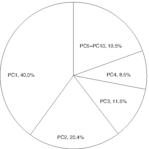
The eigenvalues of PCA. PCi (i = 1,…,10) is the ith eigenvalue. PCA, principal component analysis.

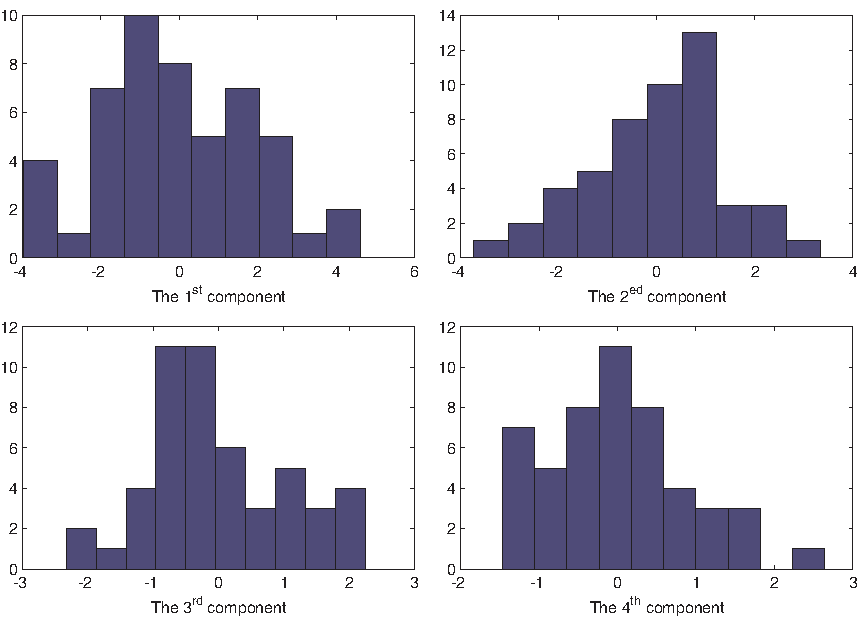
For each of the four eigenvectors e_m (d₁ ≥ d₂ ≥ d₃ ≥ d₄ ≥ d_k, k = 5,…, N_F, m = 1, 2, 3, 4), we can project \documentclass{aastex}\usepackage{amsbsy}\usepackage{amsfonts}\usepackage{amssymb}\usepackage{bm}\usepackage{mathrsfs}\usepackage{pifont}\usepackage{stmaryrd}\usepackage{textcomp}\usepackage{portland, xspace}\usepackage{amsmath, amsxtra}\usepackage{upgreek}\pagestyle{empty}\DeclareMathSizes{10}{9}{7}{6}\begin{document} $$F_{i , j}^*$$ \end{document} to e_m to form P_m,j (j = 1,…, N_WT) as (14). The histograms of 50 projected values from WT embryos on each of the four components are shown in Figure 5. To verify whether P_m,j obeys a normal distribution or not, we use Kolmogorov–Smirnov test (ks-test) (Conover, 1999). In ks-test, when we set the p value as 0.05, all the four components pass the test. Each model can be represented by two parameters as N(μ_m^WT, σ_m^WT), m = 1, 2, 3, 4.

FIG. 5.

The histogram of projected N_WT WT embryos on different components. WT, wild type.

2.5. Abnormal RNAi detection

The identification of abnormal RNAi embryos is based on the normal models built from WT embryos. First, the value of features F_i,j (i = 1,…,N_F, j = 1,…, N_RNAi, N_F = 10, N_RNAi = 136) for RNAi embryos is calculated based on the computed μ_m^WT, σ_m^WT, and e_m from WT embryos with the same way that WT embryos were treated. Second, we use Z-test according to N(μ_m^WT, σ_m^WT) and set p value as 0.05 and 0.1 to test abnormal embryos.

3. Results

The computed eigenvalues and eigenvectors in PCA are listed in Figure 4 and Table 3, respectively. According to the PCA result, the first, second, third, and fourth component, respectively, capture 40.0%, 20.4%, 11.6%, and 8.5% of the variance across all features and totally cover more than 80% of the variance. Choosing the three largest weights for the first four eigenvectors and modifying by the limitation that only one eigenvector could be assigned for a feature, the result shows that eigV1 (the eigenvector corresponding to the first eigenvalue, similarly hereinafter) mainly represents the first, third, and fifth features, which are volume mean, surface mean, diameter mean; eigV2 mainly represents the second, fourth, and sixth features, which are volume std, surface std, and diameter mean std; eigV3 mainly represents the seventh, ninth, and tenth features, which are diameter min/max mean, compactness mean, and compactness std; and eigV4 mainly represents the eighth feature, which is diameter min/max std. According to the physical meaning for each feature, it seems that the first component has strong correlation to the difference between P₁ and AB on the scale or size of a nucleus. In contrast, the second component is mainly related to the variation of scale or size of a nucleus along different time points. It may reflect the difference of development between P₁ and AB. As for the third component, it roughly reflects the geometric shape of a nucleus. Finally, the fourth component, it seems to associate with the variation of shape of a nucleus along different time points.

Table 3.

The Components of the First Four Eigenvectors

	F1	F2	F3	F4	F5	F6	F7	F8	F9	F10
eigV1	0.4292	−0.3001	0.4766	−0.0823	0.4778	0.0384	−0.2550	−0.2430	−0.2745	0.2503
eigV2	−0.1065	0.3248	−0.0119	0.5974	0.1121	0.6081	−0.1473	0.1264	−0.1546	0.2867
eigV3	0.2859	−0.1168	0.0476	0.1227	−0.0161	0.0275	0.6034	0.0001	0.5061	0.5158
eigV4	−0.0889	0.1697	−0.0473	0.3148	−0.1159	−0.1829	0.0684	−0.8993	−0.0251	−0.0319

eigV1–eigV4 represent the first four eigenvectors, and F1–F10 represent the N_F features.

After building four normal models by each of the first four components, we can use the four built models to detect RNAi embryos. For these embryos, the detection results are summarized in Table 4 and Figure 6. In Figure 6, we show the result of identification based on each of the component. To make the figures more understandable, when showing the detection result of the ith (i = 1, 2, 3, 4) component, we plot a 2D figure with ith component as x-axis and the probabilities of the value for the corresponding model as y-axis. From the result, we can draw the following conclusions:

FIG. 6.

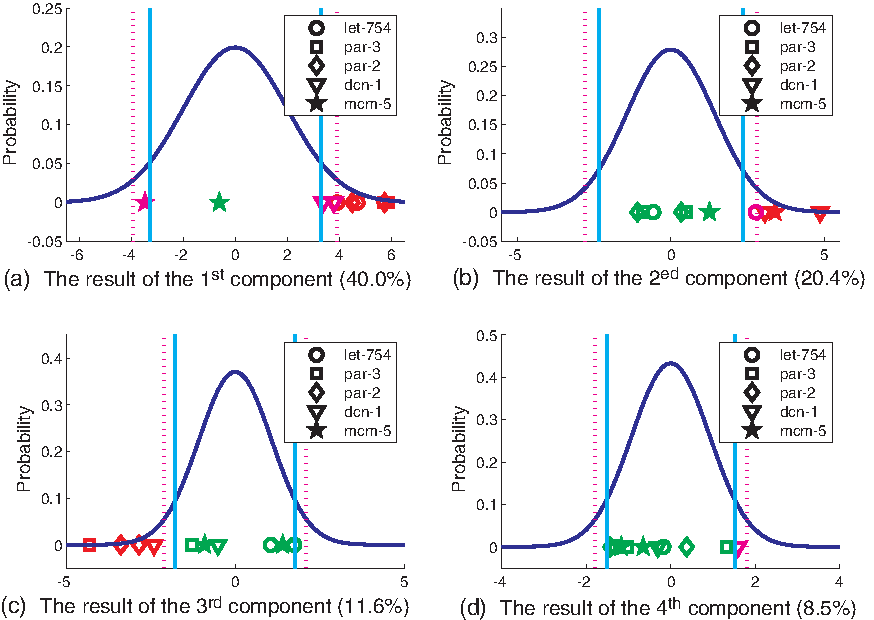
Projected 10 RNAi embryos of the five known genes (Table 1) on the ith components (i = 1, 2, 3, 4). x-Axis is the projected value and y-axis is the probability of the projected value based on the corresponding built normal distribution. The cyan solid lines and the pink dotted lines are the decision borders when p value is 0.10 and 0.05, respectively. Red objects are the projected values of embryos that are identified as abnormal cases when p value is 0.05. Pink objects are the projected values of embryos that are identified as normal cases when p value is 0.05, whereas abnormal cases when p value is 0.10. Green objects are the projected values of embryos that are identified as normal cases when p value is 0.10.

Table 4.

Detection Results for RNAi Embryos

	dcn-1		let-754		mcm-5		par-2		par-3
Gene Embryo	Embryo1	Embryo2	Embryo1	Embryo2	Embryo1	Embryo2	Embryo1	Embryo2	Embryo1	Embryo2
CDF1	0.9712	0.9542	0.9908	0.9753	0.0412	0.3805	0.9980	0.9878	0.9984	0.9978
CDF2	0.9997	0.9841	0.9742	0.3478	0.9914	0.8116	0.2243	0.5947	0.2626	0.6353
CDF3	0.3170	0.0126	0.8374	0.9478	0.9040	0.2002	0.0008	0.0040	0.0000	0.1181
CDF4	0.3703	0.9579	0.0791	0.4250	0.1019	0.2404	0.6599	0.0606	0.9240	0.1290

CDF1–CDF4 represent the cumulative distribution function of testing for an embryo when m is 1, 2, 3, and 4. Bold values correspond to abnormal embryos, which are detected when p value is 0.05, and values with an italic font correspond to abnormal embryos when p value is 0.1.

First, let-754, par-2, and par-3 play important roles in the asymmetric division on scale, because silencing one of them tends to change the difference of P₁ and AB on scale. The knockdown of dcn-1 by RNAi arguably changes the division similar to the former three genes, whereas the knockdown of mcm-5 arguably changes the division in an opposite way.

Second, the genes, dcn-1 and mcm-5, are crucial in the asymmetric division on the change of scale (we guess it is related to the growth ratio), because silencing one of them tends to change the difference of P₁ and AB on the variation of scale or size of a nucleus along different time points. The gene, let-754, arguably has the same function, whereas par-2 and par-3 have negligible influence on the variation of scale.

Third, dcn-1, par-2, and par-3 serve important functions in the asymmetric division on geometric shape, because silencing one of them tends to change the difference of P₁ and AB on geometric shape.

4. Conclusions

We propose a framework to identify gene functions in this article. To validate the framework, we apply it to identify the concrete functions of five known genes appearing both in Phenobank and in WDDD, which are critical in the asymmetric division of C. elegans on the first round. Experimental results show the effectiveness of this framework in identifying specific gene functions for certain category of abnormal phenotypes. Because the scheme introduced in this study can be applied to other genes making only few modifications, it may have extensive applications. One requirement of the method is that it needs a large number of WT embryos to build reliable models.

Footnotes

Acknowledgments

This work was supported, in part, by the National Bioscience Database Center (NBDC) of the Japan Science and Technology Agency (JST), the Strategic Programs for R&D (President's Discretionary Fund) of RIKEN, and the Grant-in-aid for Scientific Research from the Japanese Ministry for Education, Science, Culture, and Sports (MEXT) under the Grant No. 16H01436.

Author Disclosure Statement

No competing financial interests exist.

References

Arata

, Takagi

, Sako , et al. 2015. Power low relationship between cell cycle duration and cell volume in the early embryonic development of Caenorhabditis elegans. Front. Physiol., 5, 529.

Ashrafi

, Chang

F.Y.

, Watts

J.L.

, et al. 2003. Genome-wide RNAi analysis of Caenorhabditis elegans fat regulatory genes. Nature, 421, 268–272.

Attneave

, and Arnoult

M.D.

1956. The quantitative study of shape and pattern perception. Psychol. Bull., 53, 452–471.

Bai

, Binari

, Ni

J.Q.

, et al. 2008. RNA interference screening in Drosophila primary cells for genes involved in muscle assembly and maintenance. Development, 135, 1439–1449.

Betschinger

, and Knoblich

2004. Dare to be different: Asymmetric cell division in Drosophila, C. elegans and vertebrates. Curr. Biol., 14, 674–685.

Conover

W.J.

1999. Practical Nonparametric Statistics. 3rd ed. John Wiley & Sons, New York.

Fraser

A.G.

, Kamath

R.S.

, Zipperlen

, et al. 2000. Functional genomic analysis of C. elegans chromosome I by systematic RNA interference. Nature, 408, 325–330.

, Uauy

, Blechl

, et al. 2007. RNA interference for wheat functional gene analysis. Transgenic Res. 16, 689–701.

Glasbey

C.A.

, and Horgan

G.W.

1995. Image Analysis for the Biological Sciences. John Wiley & Sons, New York.

10.

Gönczy

2008. Mechanisms of asymmetric cell division: Flies and worms pave the way. Nat. Rev. Mol. Cell Biol., 9, 355–366.

11.

Guo

S.1.

, and Kemphues

K.J.

1995. par-1, a gene required for establishing polarity in C. elegans embryos, encodes a putative Ser/Thr kinase that is asymmetrically distributed. Cell, 81, 611–620.

12.

Hamahashi

, Kitano

, and Onami

2007. A system for measuring cell division patterns of early Caenorhabditis elegans embryos by using image processing and object tracking. Syst. Comput. Jpn., 38, 12–24.

13.

Hara

, Iwabuchi

, Ohsumi

, et al. 2013. Intranuclear DNA density affects chromosome condensation in metazoans. Mol. Biol. Cell, 24, 2442–2453.

14.

Horvitz

H.R.

, and Herskowitz

1992. Mechanisms of asymmetric cell division: Two Bs or not two Bs, that is the question. Cell, 68, 237–255.

15.

Kemphues

K.J.

, Priess

J.R.

, Morton

D.G.

, et al. 1988. Identification of genes requires for cytoplasmic localization in early C. elegans embryos. Cell, 52, 311–320.

16.

Kyoda

, Adachi

, Masuda

, et al. 2013. WDDD: Worm Developmental Dynamics Database. Nucleic Acids Res. 41, 732–737.

17.

Ladouceur

A.M.

, Dorn

J.F.

, and Maddox

P.S.

2015. Mitotic chromosome length scales in response to both cell and nuclear size. J. Cell Biol., 209, 645–651.

18.

Loncaric

1998. A survey of shape analysis techniques. Pattern Recognit. 31, 983–1001.

19.

Neumüller

R.A.

, and Perrimon

2011. Where gene discovery turns into systems biology: Genome-scale RNAi screens in Drosophila. Wiley Interdiscip. Rev. Syst. Biol. Med., 3, 471–478.

20.

Rosenfeld

1974. Compact figures in digital pictures. IEEE Trans. Syst. Man Cybern. SMC-4, 221–223.

21.

Sönnichsen

, Koski

L.B.

, Walsh

, et al. 2005. Full-genome RNAi profiling of early embryogenesis in Caenorhabditis elegans. Nature, 434, 462–469.

22.

Sulston

J.E.

, Schierenberg

, White

J.G.

, et al. 1983. The embryonic cell lineage of the nematode Caenorhabditis elegans. Dev. Biol., 100, 64–119.

23.

Treeby

B.E.

, and Cox

B.T.

2010. k-Wave: MATLAB toolbox for the simulation and reconstruction of photoacoustic wave fields. J. Biomed. Opt., 15, 021314.

24.

Young

I.T.

, Walker

J.E.

, and Bowie

J.E.

1974. An analysis technique for biological shape. I. Inf. Control, 25, 357–370.

25.

Zhang

, and Lu

2004. Review of shape representation and description techniques. Pattern Recognit. 37, 1–19.