In human genome research, genetic association studies of rare variants have been widely studied since the advent of high-throughput DNA sequencing platforms. However, detection of outcome-related rare variants still remains a statistically challenging problem because the number of observed genetic mutations is extremely rare. Recently, a power set-based statistical selection procedure has been proposed to locate both risk and protective rare variants within the outcome-related genes or genetic regions. Although it can perform an individual selection of rare variants, the procedure has a limitation that it cannot measure the certainty of selected rare variants. In this article, we propose a selection probability of individual rare variants, where selection frequencies of rare variants are computed based on bootstrap resampling. Therefore, it can quantify the certainty of both selected and unselected rare variants. Also, a new selection approach using a threshold of selection probability is introduced and compared with some existing selection procedures from extensive simulation studies and real sequencing data analysis. We have demonstrated that the proposed approach outperforms the existing methods in terms of a selection power.
1. Introduction
In postgenome-wide association studies, rare variants (with minor allele frequency [MAF] <1%) have been expected that they can explain missing heritability of complex diseases and traits that have not been captured by common variant analysis (Manolio et al., 2009; Lander, 2011; Zuk et al., 2012). However, detection of outcome-related rare variants still remains a statistically challenging problem because of the limited number of genetic mutations for individual variants. In this reason, most of existing statistical methods to detect rare variants associated with either a complex disease or trait have been developed as a gene-based group test, where a group of multiple rare variants within the same gene or the same genetic regions is tested if the group is significantly associated with a phenotype outcome (Liu and Leal, 2010; Price et al., 2010; Lin and Tang, 2011; Wu et al., 2011; Lee et al., 2012, 2014; Ionita-Laza et al., 2013, 2014; Sun et al., 2013). For example, the sequence kernel association test (SKAT) uses the kernel machine regression, aggregating individual rare variants (Wu et al., 2011). The optimal unified test (SKAT-O) is based on a weighted linear combination of a burden test and the SKAT variance component test (Lee et al., 2012). The mixed effects score test has broadened the use of variance component score statistics of multiple variants (Sun et al., 2013).
However, these group association tests have a limitation that they cannot locate the outcome-related rare variants in the group. If one of the gene-based group tests detects that a gene or a genetic region is significantly associated with a phenotype outcome, identification of outcome-related variants in the gene or the genetic region will be of interest in the next step. Recently, a few of rare variant selection methods have been proposed to separate both risk and protective variants from noncausal variants in the same group. Specifically, a backward elimination procedure using the p values of a burden test and SKAT can perform both a group association test and variant selection at the same time (Ionita-Laza et al., 2014). A power set-based statistical selection procedure (Pset) that is based on a weighted linear combination of rare variants has been proposed to identify both risk and protective rare variants within the outcome-related genes (Sun and Wang, 2014). In a similar manner, a new selection strategy with a forward selection procedure was suggested to increase true positive rates of protective rare variants, reducing computational time for large genes (Kim et al., 2015).
Although the existing rare variant selection procedures show a relatively powerful selection performance, they do not provide the certainty of selected rare variants. As their selection result of individual rare variants is just summarized as either selected or not selected, we cannot measure association strength of selected variants from the existing selection procedures. It is well known that marginal association tests of individual rare variants are seriously underpowered because of extremely rare observations of genetic mutations. In this article, we propose a selection probability of individual rare variants, so that the certainty of both selected and unselected variants can be quantified. Based on the selection probability, we can not only compare the association strength of selected variants with each other but can also compare unselected variants with each other, where some could be potentially true negatives. In addition to selection probability, we suggest a new selection approach using a threshold of the selection probability, where individual variants are selected if their selection probability is greater than the threshold.
The rest of this article is organized as follows. In Section 2, we first briefly review the Pset method, in which the proposed selection probability has been applied to. Next, the selection probability and new selection approach using a threshold are described. In Section 3, we validated the proposed selection probability of individual variants from simulation studies. Also, we demonstrated that the proposed selection approach outperforms the Pset method through extensive simulation studies, where various simulation scenarios were considered. In Section 4, rare variant selection results for real sequencing data are presented, where we applied the proposed selection probability and selection approach to the Dallas Heart Study (DHS) data. Finally, Section 5 summarizes this article and outlines future research work.
2. Methods
Suppose that we have a data set of the i-th individual consisting of \documentclass{aastex}\usepackage{amsbsy}\usepackage{amsfonts}\usepackage{amssymb}\usepackage{bm}\usepackage{mathrsfs}\usepackage{pifont}\usepackage{stmaryrd}\usepackage{textcomp}\usepackage{portland, xspace}\usepackage{amsmath, amsxtra}\usepackage{upgreek}\pagestyle{empty}\DeclareMathSizes{10}{9}{7}{6}\begin{document}
$$( {x_i} , {y_i} , {u_i} )$$
\end{document} for \documentclass{aastex}\usepackage{amsbsy}\usepackage{amsfonts}\usepackage{amssymb}\usepackage{bm}\usepackage{mathrsfs}\usepackage{pifont}\usepackage{stmaryrd}\usepackage{textcomp}\usepackage{portland, xspace}\usepackage{amsmath, amsxtra}\usepackage{upgreek}\pagestyle{empty}\DeclareMathSizes{10}{9}{7}{6}\begin{document}
$$i = 1 , \ldots , n$$
\end{document}, where \documentclass{aastex}\usepackage{amsbsy}\usepackage{amsfonts}\usepackage{amssymb}\usepackage{bm}\usepackage{mathrsfs}\usepackage{pifont}\usepackage{stmaryrd}\usepackage{textcomp}\usepackage{portland, xspace}\usepackage{amsmath, amsxtra}\usepackage{upgreek}\pagestyle{empty}\DeclareMathSizes{10}{9}{7}{6}\begin{document}
$${x_i} = ( {x_{i1}} , \ldots , {x_{ip}}{ ) ^{ \rm{T}}}$$
\end{document} is the p-dimensional vector representing the number of minor alleles contained in the genotype over the p rare variants, yi is a phenotype outcome that can be either quantitative or binary such as case–control status, and \documentclass{aastex}\usepackage{amsbsy}\usepackage{amsfonts}\usepackage{amssymb}\usepackage{bm}\usepackage{mathrsfs}\usepackage{pifont}\usepackage{stmaryrd}\usepackage{textcomp}\usepackage{portland, xspace}\usepackage{amsmath, amsxtra}\usepackage{upgreek}\pagestyle{empty}\DeclareMathSizes{10}{9}{7}{6}\begin{document}
$${u_i} = ( {u_{i1}} , \ldots , {u_{im}}{ ) ^{ \rm{T}}}$$
\end{document} is the m-dimensional covariate vector such as age and gender. When covariates are present, the regression residuals \documentclass{aastex}\usepackage{amsbsy}\usepackage{amsfonts}\usepackage{amssymb}\usepackage{bm}\usepackage{mathrsfs}\usepackage{pifont}\usepackage{stmaryrd}\usepackage{textcomp}\usepackage{portland, xspace}\usepackage{amsmath, amsxtra}\usepackage{upgreek}\pagestyle{empty}\DeclareMathSizes{10}{9}{7}{6}\begin{document}
$${ \tilde y_i}$$
\end{document} for \documentclass{aastex}\usepackage{amsbsy}\usepackage{amsfonts}\usepackage{amssymb}\usepackage{bm}\usepackage{mathrsfs}\usepackage{pifont}\usepackage{stmaryrd}\usepackage{textcomp}\usepackage{portland, xspace}\usepackage{amsmath, amsxtra}\usepackage{upgreek}\pagestyle{empty}\DeclareMathSizes{10}{9}{7}{6}\begin{document}
$$i = 1 , \ldots , n ,$$
\end{document} are first computed from either a liner regression for a quantitative yi or a logistic regression for a case–control yi, where \documentclass{aastex}\usepackage{amsbsy}\usepackage{amsfonts}\usepackage{amssymb}\usepackage{bm}\usepackage{mathrsfs}\usepackage{pifont}\usepackage{stmaryrd}\usepackage{textcomp}\usepackage{portland, xspace}\usepackage{amsmath, amsxtra}\usepackage{upgreek}\pagestyle{empty}\DeclareMathSizes{10}{9}{7}{6}\begin{document}
$${y_i} = 0$$
\end{document} for a control and \documentclass{aastex}\usepackage{amsbsy}\usepackage{amsfonts}\usepackage{amssymb}\usepackage{bm}\usepackage{mathrsfs}\usepackage{pifont}\usepackage{stmaryrd}\usepackage{textcomp}\usepackage{portland, xspace}\usepackage{amsmath, amsxtra}\usepackage{upgreek}\pagestyle{empty}\DeclareMathSizes{10}{9}{7}{6}\begin{document}
$${y_i} = 1$$
\end{document} for a case. These residuals from the regression fit, where a phenotype outcome is on the response and the m covariates are on the predictors, can isolate the genetic effect of xi on the outcome because they remove the covariate effect on the phenotype outcome. If no covariates are present, \documentclass{aastex}\usepackage{amsbsy}\usepackage{amsfonts}\usepackage{amssymb}\usepackage{bm}\usepackage{mathrsfs}\usepackage{pifont}\usepackage{stmaryrd}\usepackage{textcomp}\usepackage{portland, xspace}\usepackage{amsmath, amsxtra}\usepackage{upgreek}\pagestyle{empty}\DeclareMathSizes{10}{9}{7}{6}\begin{document}
$${ \tilde y_i} = {y_i}$$
\end{document}.
2.1. A power set-based selection
The Pset method (Sun and Wang, 2014) based on a weighted linear combination of p rare variants considers all of the \documentclass{aastex}\usepackage{amsbsy}\usepackage{amsfonts}\usepackage{amssymb}\usepackage{bm}\usepackage{mathrsfs}\usepackage{pifont}\usepackage{stmaryrd}\usepackage{textcomp}\usepackage{portland, xspace}\usepackage{amsmath, amsxtra}\usepackage{upgreek}\pagestyle{empty}\DeclareMathSizes{10}{9}{7}{6}\begin{document}
$${2^p} - 1$$
\end{document} subsets of the power set of the variants and finds the best combination among the p variants that has the maximum association signal with a phenotype outcome. Specifically, the new feature for the subset k of the i-th individual is defined as
\documentclass{aastex}\usepackage{amsbsy}\usepackage{amsfonts}\usepackage{amssymb}\usepackage{bm}\usepackage{mathrsfs}\usepackage{pifont}\usepackage{stmaryrd}\usepackage{textcomp}\usepackage{portland, xspace}\usepackage{amsmath, amsxtra}\usepackage{upgreek}\pagestyle{empty}\DeclareMathSizes{10}{9}{7}{6}\begin{document}
\begin{align*}
{z_{ik}} = \mathop \sum \limits_{j = 1}^p { \xi _{kj}}{ \omega _j}{x_{ij}} , ( 1 )
\end{align*}
\end{document}
where \documentclass{aastex}\usepackage{amsbsy}\usepackage{amsfonts}\usepackage{amssymb}\usepackage{bm}\usepackage{mathrsfs}\usepackage{pifont}\usepackage{stmaryrd}\usepackage{textcomp}\usepackage{portland, xspace}\usepackage{amsmath, amsxtra}\usepackage{upgreek}\pagestyle{empty}\DeclareMathSizes{10}{9}{7}{6}\begin{document}
$${ \omega _j} > 0$$
\end{document} is the user-defined weight of the j-th variant and \documentclass{aastex}\usepackage{amsbsy}\usepackage{amsfonts}\usepackage{amssymb}\usepackage{bm}\usepackage{mathrsfs}\usepackage{pifont}\usepackage{stmaryrd}\usepackage{textcomp}\usepackage{portland, xspace}\usepackage{amsmath, amsxtra}\usepackage{upgreek}\pagestyle{empty}\DeclareMathSizes{10}{9}{7}{6}\begin{document}
$${ \xi _k} = ( { \xi _{k1}} , \ldots , { \xi _{kp}}{ ) ^{ \rm{T}}}$$
\end{document} is the the p-dimensional weighting vector for the subset k, coding \documentclass{aastex}\usepackage{amsbsy}\usepackage{amsfonts}\usepackage{amssymb}\usepackage{bm}\usepackage{mathrsfs}\usepackage{pifont}\usepackage{stmaryrd}\usepackage{textcomp}\usepackage{portland, xspace}\usepackage{amsmath, amsxtra}\usepackage{upgreek}\pagestyle{empty}\DeclareMathSizes{10}{9}{7}{6}\begin{document}
$${ \xi _{kj}} = 1$$
\end{document} if the j-th rare variant is included in the subset k and otherwise \documentclass{aastex}\usepackage{amsbsy}\usepackage{amsfonts}\usepackage{amssymb}\usepackage{bm}\usepackage{mathrsfs}\usepackage{pifont}\usepackage{stmaryrd}\usepackage{textcomp}\usepackage{portland, xspace}\usepackage{amsmath, amsxtra}\usepackage{upgreek}\pagestyle{empty}\DeclareMathSizes{10}{9}{7}{6}\begin{document}
$${ \xi _{kj}} = 0$$
\end{document}. In general, the Pset shows powerful selection performance except when both risk and protective variants are present in the same gene or genetic region. As risk and protective variants have different direction effects on the outcome of each other, the weighted linear combination of these variants is likely to fail to locate them.
Alternatively, a data adaptive power set (aPset) selection procedure can be applied to identify both risk and protective variants. The aPset method first screens potentially protective variants using a marginal association test. It then flips the coding of the potentially protective variants so that linearly combined both risk and protective variants can have the same direction effects on the phenotype outcome. To generate the new feature of the aPset method, we just need to replace \documentclass{aastex}\usepackage{amsbsy}\usepackage{amsfonts}\usepackage{amssymb}\usepackage{bm}\usepackage{mathrsfs}\usepackage{pifont}\usepackage{stmaryrd}\usepackage{textcomp}\usepackage{portland, xspace}\usepackage{amsmath, amsxtra}\usepackage{upgreek}\pagestyle{empty}\DeclareMathSizes{10}{9}{7}{6}\begin{document}
$${x_{ij}}$$
\end{document} in Equation (1) by \documentclass{aastex}\usepackage{amsbsy}\usepackage{amsfonts}\usepackage{amssymb}\usepackage{bm}\usepackage{mathrsfs}\usepackage{pifont}\usepackage{stmaryrd}\usepackage{textcomp}\usepackage{portland, xspace}\usepackage{amsmath, amsxtra}\usepackage{upgreek}\pagestyle{empty}\DeclareMathSizes{10}{9}{7}{6}\begin{document}
$$x_{ij}^*$$
\end{document}, which is defined as
\documentclass{aastex}\usepackage{amsbsy}\usepackage{amsfonts}\usepackage{amssymb}\usepackage{bm}\usepackage{mathrsfs}\usepackage{pifont}\usepackage{stmaryrd}\usepackage{textcomp}\usepackage{portland, xspace}\usepackage{amsmath, amsxtra}\usepackage{upgreek}\pagestyle{empty}\DeclareMathSizes{10}{9}{7}{6}\begin{document}
\begin{align*}
x_{ij}^* = \left\{ { \begin{matrix} {1 - {x_{ij}}} \hfill & {{ \rm{if \ the \ }}j{ \rm{ - th \ variant \ is \ protective , }}} \hfill \\ {{x_{ij}}} \hfill & {{ \rm{otherwise}}{ \rm{.}}} \hfill \\ \end{matrix} } \right.
\end{align*}
\end{document}
To find the feature that has the maximum association signal with a phenotype outcome among \documentclass{aastex}\usepackage{amsbsy}\usepackage{amsfonts}\usepackage{amssymb}\usepackage{bm}\usepackage{mathrsfs}\usepackage{pifont}\usepackage{stmaryrd}\usepackage{textcomp}\usepackage{portland, xspace}\usepackage{amsmath, amsxtra}\usepackage{upgreek}\pagestyle{empty}\DeclareMathSizes{10}{9}{7}{6}\begin{document}
$$K{ = 2^p} - 1$$
\end{document} features, we test each feature \documentclass{aastex}\usepackage{amsbsy}\usepackage{amsfonts}\usepackage{amssymb}\usepackage{bm}\usepackage{mathrsfs}\usepackage{pifont}\usepackage{stmaryrd}\usepackage{textcomp}\usepackage{portland, xspace}\usepackage{amsmath, amsxtra}\usepackage{upgreek}\pagestyle{empty}\DeclareMathSizes{10}{9}{7}{6}\begin{document}
$${z_{ik}}$$
\end{document} for association with the residual \documentclass{aastex}\usepackage{amsbsy}\usepackage{amsfonts}\usepackage{amssymb}\usepackage{bm}\usepackage{mathrsfs}\usepackage{pifont}\usepackage{stmaryrd}\usepackage{textcomp}\usepackage{portland, xspace}\usepackage{amsmath, amsxtra}\usepackage{upgreek}\pagestyle{empty}\DeclareMathSizes{10}{9}{7}{6}\begin{document}
$${ \tilde y_i}$$
\end{document} and find
\documentclass{aastex}\usepackage{amsbsy}\usepackage{amsfonts}\usepackage{amssymb}\usepackage{bm}\usepackage{mathrsfs}\usepackage{pifont}\usepackage{stmaryrd}\usepackage{textcomp}\usepackage{portland, xspace}\usepackage{amsmath, amsxtra}\usepackage{upgreek}\pagestyle{empty}\DeclareMathSizes{10}{9}{7}{6}\begin{document}
\begin{align*}
\hat k = \mathop { \arg \max } \limits_{1 \le k \le K} T ( \tilde y , {z_k} ) ,
\end{align*}
\end{document}
where \documentclass{aastex}\usepackage{amsbsy}\usepackage{amsfonts}\usepackage{amssymb}\usepackage{bm}\usepackage{mathrsfs}\usepackage{pifont}\usepackage{stmaryrd}\usepackage{textcomp}\usepackage{portland, xspace}\usepackage{amsmath, amsxtra}\usepackage{upgreek}\pagestyle{empty}\DeclareMathSizes{10}{9}{7}{6}\begin{document}
$$\tilde y = ( { \tilde y_1} , \ldots , { \tilde y_n}{ ) ^{ \rm{T}}}$$
\end{document} and \documentclass{aastex}\usepackage{amsbsy}\usepackage{amsfonts}\usepackage{amssymb}\usepackage{bm}\usepackage{mathrsfs}\usepackage{pifont}\usepackage{stmaryrd}\usepackage{textcomp}\usepackage{portland, xspace}\usepackage{amsmath, amsxtra}\usepackage{upgreek}\pagestyle{empty}\DeclareMathSizes{10}{9}{7}{6}\begin{document}
$${z_k} = ( {z_{1k}} , \ldots , {z_{nk}}{ ) ^{ \rm{T}}}$$
\end{document}, and \documentclass{aastex}\usepackage{amsbsy}\usepackage{amsfonts}\usepackage{amssymb}\usepackage{bm}\usepackage{mathrsfs}\usepackage{pifont}\usepackage{stmaryrd}\usepackage{textcomp}\usepackage{portland, xspace}\usepackage{amsmath, amsxtra}\usepackage{upgreek}\pagestyle{empty}\DeclareMathSizes{10}{9}{7}{6}\begin{document}
$$T ( a , b )$$
\end{document} is a statistic to measure an association between a and b. The Pset and aPset methods used a sample correlation in \documentclass{aastex}\usepackage{amsbsy}\usepackage{amsfonts}\usepackage{amssymb}\usepackage{bm}\usepackage{mathrsfs}\usepackage{pifont}\usepackage{stmaryrd}\usepackage{textcomp}\usepackage{portland, xspace}\usepackage{amsmath, amsxtra}\usepackage{upgreek}\pagestyle{empty}\DeclareMathSizes{10}{9}{7}{6}\begin{document}
$$T ( a , b )$$
\end{document} for computational speed up.
2.2. Selection probability
The selection result of the Pset and aPset methods is summarized as either selected or unselected for each variant. So, we cannot measure the certainty of both selected and unselected variants. Selection probability of individual variables was originally proposed for regularization methods such as a least absolute shrinkage and selection operator (lasso) and penalized Gaussian graphical models (Meinshausen and Bühlmann, 2010). The idea of selection probability was inspired by stable selection of high-dimensional data because cross-validation studies to validate a tuning parameter for regularization often result in unstable variable selection. Also, it has been applied to rank selected genes from the largest selection probability to the smallest selection probability for analysis of high-dimensional genomic data (Alexander and Lange, 2011; Sun and Wang, 2012, 2013). Selection probability used in the literature was computed based on repeatedly selected half of samples without replacement. However, observed genetic data in rare variant analysis consist of most of homozygous genotypes and extremely rare heterozygous genotypes. So, resampling of half of samples frequently includes only homozygous genotypes, where variable selection cannot be performed. In this reason, we employ a nonparametric bootstrap resampling to compute selection probability of individual rare variants.
Given n individuals (with either a quantitative or a case–control binary), we randomly resample n individuals with replacement and obtain a new data set consisting of \documentclass{aastex}\usepackage{amsbsy}\usepackage{amsfonts}\usepackage{amssymb}\usepackage{bm}\usepackage{mathrsfs}\usepackage{pifont}\usepackage{stmaryrd}\usepackage{textcomp}\usepackage{portland, xspace}\usepackage{amsmath, amsxtra}\usepackage{upgreek}\pagestyle{empty}\DeclareMathSizes{10}{9}{7}{6}\begin{document}
$$( {x_{{i^*}}} , {y_{{i^*}}} , {u_{{i^*}}} ) ,$$
\end{document} where \documentclass{aastex}\usepackage{amsbsy}\usepackage{amsfonts}\usepackage{amssymb}\usepackage{bm}\usepackage{mathrsfs}\usepackage{pifont}\usepackage{stmaryrd}\usepackage{textcomp}\usepackage{portland, xspace}\usepackage{amsmath, amsxtra}\usepackage{upgreek}\pagestyle{empty}\DeclareMathSizes{10}{9}{7}{6}\begin{document}
$$1 \le {i^*} \le n$$
\end{document} is the i-th resampled individual. One key feature of the nonparametric bootstrap is that sampled individuals have their phenotype outcome and genetic information intact. We then apply either the Pset or the aPset method to identify the most outcome-related subset of rare variants on the resampled n subjects. Denote the selection result of the \documentclass{aastex}\usepackage{amsbsy}\usepackage{amsfonts}\usepackage{amssymb}\usepackage{bm}\usepackage{mathrsfs}\usepackage{pifont}\usepackage{stmaryrd}\usepackage{textcomp}\usepackage{portland, xspace}\usepackage{amsmath, amsxtra}\usepackage{upgreek}\pagestyle{empty}\DeclareMathSizes{10}{9}{7}{6}\begin{document}
$$\upsilon$$
\end{document}-th bootstrap sample as \documentclass{aastex}\usepackage{amsbsy}\usepackage{amsfonts}\usepackage{amssymb}\usepackage{bm}\usepackage{mathrsfs}\usepackage{pifont}\usepackage{stmaryrd}\usepackage{textcomp}\usepackage{portland, xspace}\usepackage{amsmath, amsxtra}\usepackage{upgreek}\pagestyle{empty}\DeclareMathSizes{10}{9}{7}{6}\begin{document}
$$( s_1^ \upsilon , s_2^ \upsilon , \ldots , s_p^ \upsilon )$$
\end{document}, \documentclass{aastex}\usepackage{amsbsy}\usepackage{amsfonts}\usepackage{amssymb}\usepackage{bm}\usepackage{mathrsfs}\usepackage{pifont}\usepackage{stmaryrd}\usepackage{textcomp}\usepackage{portland, xspace}\usepackage{amsmath, amsxtra}\usepackage{upgreek}\pagestyle{empty}\DeclareMathSizes{10}{9}{7}{6}\begin{document}
$$\upsilon = 1 , \ldots , M$$
\end{document}, where \documentclass{aastex}\usepackage{amsbsy}\usepackage{amsfonts}\usepackage{amssymb}\usepackage{bm}\usepackage{mathrsfs}\usepackage{pifont}\usepackage{stmaryrd}\usepackage{textcomp}\usepackage{portland, xspace}\usepackage{amsmath, amsxtra}\usepackage{upgreek}\pagestyle{empty}\DeclareMathSizes{10}{9}{7}{6}\begin{document}
$$s_j^ \upsilon = 1$$
\end{document} if variant j is selected and \documentclass{aastex}\usepackage{amsbsy}\usepackage{amsfonts}\usepackage{amssymb}\usepackage{bm}\usepackage{mathrsfs}\usepackage{pifont}\usepackage{stmaryrd}\usepackage{textcomp}\usepackage{portland, xspace}\usepackage{amsmath, amsxtra}\usepackage{upgreek}\pagestyle{empty}\DeclareMathSizes{10}{9}{7}{6}\begin{document}
$$s_j^ \upsilon = 0$$
\end{document} if variant j is not selected. The selection probability of variant j can be calculated as
\documentclass{aastex}\usepackage{amsbsy}\usepackage{amsfonts}\usepackage{amssymb}\usepackage{bm}\usepackage{mathrsfs}\usepackage{pifont}\usepackage{stmaryrd}\usepackage{textcomp}\usepackage{portland, xspace}\usepackage{amsmath, amsxtra}\usepackage{upgreek}\pagestyle{empty}\DeclareMathSizes{10}{9}{7}{6}\begin{document}
\begin{align*}
{ \rm { S } } { { \rm { P } } _j } = \frac { 1 } { { { M_j } } } \mathop \sum \limits_ { \upsilon = 1 } ^M s_j^ \upsilon ,
\end{align*}
\end{document}
where \documentclass{aastex}\usepackage{amsbsy}\usepackage{amsfonts}\usepackage{amssymb}\usepackage{bm}\usepackage{mathrsfs}\usepackage{pifont}\usepackage{stmaryrd}\usepackage{textcomp}\usepackage{portland, xspace}\usepackage{amsmath, amsxtra}\usepackage{upgreek}\pagestyle{empty}\DeclareMathSizes{10}{9}{7}{6}\begin{document}
$${M_j} \le M$$
\end{document} is the total number of bootstrap samples that have at least one heterozygous genotype observed at variant j. This is because of bootstrap resampling with replacement, some variants can have only homozygous genotypes in a particular bootstrap sample. In this case, we have to exclude the variants from the analysis because at least one genetic mutation among n samples is required to apply the Pset or the aPest method. Therefore, the total number of effective bootstrap samples for each variant may vary. As the selection probability for an individual variant is quickly stabilized as M increases, usually M = 200 is enough to obtain the selection probabilities.
Selection probability of each variant represents a relative selection frequency of an individual variant through repeated sampling. As we can compare the selection probabilities for all variants in a gene or a genetic region, it can be used to quantify the certainty of both selected and unselected rare variants. Although a selection probability for an individual variant is helpful to assess statistical confidence of the selection results, they can be used only as a relative measurement across all rare variants in a gene or a genetic region. It is a separate statistical problem to test whether selected variants are significantly associated with a phenotype outcome. Therefore, we recommend to do a stage I association test with any of the existing test procedures (Liu and Leal, 2010; Price et al., 2010; Lin and Tang, 2011; Wu et al., 2011; Lee et al., 2012, 2014; Ionita-Laza et al., 2013, 2014; Sun et al., 2013) so that a gene or a genetic region with rare variants is first identified to be associated with the outcome. We then apply the selection procedure to locate susceptible rare variants within the gene or the genetic region together with the selection probabilities provided.
2.3. New selection approach
Although the Pset and aPset methods can find the best combination of rare variants that has the maximum association signal with a phenotype outcome, they often produce relatively many false positives when either a variant effect size or a sample size is small. Alternative to the Pset and aPset methods, we introduce a new selection approach that is able to control the number of selected variants. The new selection approach is based on a threshold of selection probabilities of individual rare variants, where variant j is selected only if \documentclass{aastex}\usepackage{amsbsy}\usepackage{amsfonts}\usepackage{amssymb}\usepackage{bm}\usepackage{mathrsfs}\usepackage{pifont}\usepackage{stmaryrd}\usepackage{textcomp}\usepackage{portland, xspace}\usepackage{amsmath, amsxtra}\usepackage{upgreek}\pagestyle{empty}\DeclareMathSizes{10}{9}{7}{6}\begin{document}
$${ \rm{S}}{{ \rm{P}}_j} > \alpha$$
\end{document} for a threshold \documentclass{aastex}\usepackage{amsbsy}\usepackage{amsfonts}\usepackage{amssymb}\usepackage{bm}\usepackage{mathrsfs}\usepackage{pifont}\usepackage{stmaryrd}\usepackage{textcomp}\usepackage{portland, xspace}\usepackage{amsmath, amsxtra}\usepackage{upgreek}\pagestyle{empty}\DeclareMathSizes{10}{9}{7}{6}\begin{document}
$$0 \le \alpha \le 1.$$
\end{document} For a larger value of α, less variants are selected so both true and false positives are decreased. In contrast, more rare variants are selected as α decreases, where both true and false positives are increased at the same time. Therefore, the threshold α can control the size of the selected subset of rare variants, which leads to different number of true positives (risk and protective variants) and false positives (noncausal variants).
The optimal choice of α is very challenging, because it might depend on a sample size, a gene size, a variant effect size, and the number of risk and protective variants in the gene. In our extensive simulation studies, we first set a fine grid of α between 0 and 1 and apply the proposed selection approach with each α for various simulation scenarios, where three different sample sizes, six different variant effect sizes, and two different numbers of risk and protective variants were considered. We discovered that the proposed selection approach with α = 0.6 has overall shown superior selection power in various scenarios.
3. Simulation Studies
We have conducted three different types of simulation studies. The first simulation is to validate selection probabilities of risk, protective, and noncausal variants, where selection probabilities of individual rare variants were compared with each other. In the second simulation, the proposed selection approach based on the threshold α = 0.6 of selection probabilities was compared with the existing selection methods in terms of average selection proportions (ASPs) of risk, protective and noncausal variants, and selection power. In the last simulation study, the selection power of the proposed selection approach was investigated along with a different value of a threshold α.
In our three simulation studies, we have generated genotype data and phenotype data in the same way. First, MAFs for p rare variants were randomly generated from a Wright's distribution (Madsen and Browning, 2009; Ionita-Laza et al., 2011; Sun and Wang, 2014; Kim et al., 2015). Next, we generated genotype data \documentclass{aastex}\usepackage{amsbsy}\usepackage{amsfonts}\usepackage{amssymb}\usepackage{bm}\usepackage{mathrsfs}\usepackage{pifont}\usepackage{stmaryrd}\usepackage{textcomp}\usepackage{portland, xspace}\usepackage{amsmath, amsxtra}\usepackage{upgreek}\pagestyle{empty}\DeclareMathSizes{10}{9}{7}{6}\begin{document}
$${x_i} = ( {x_{i1}} , \cdots , {x_{ip}} )$$
\end{document} of the i-th individual on the basis of the Hardy–Weinberg equilibrium. Finally, we computed a quantitative phenotype value yi of the i-th individual by using the following multiple linear regression model
\documentclass{aastex}\usepackage{amsbsy}\usepackage{amsfonts}\usepackage{amssymb}\usepackage{bm}\usepackage{mathrsfs}\usepackage{pifont}\usepackage{stmaryrd}\usepackage{textcomp}\usepackage{portland, xspace}\usepackage{amsmath, amsxtra}\usepackage{upgreek}\pagestyle{empty}\DeclareMathSizes{10}{9}{7}{6}\begin{document}
\begin{align*}
{y_i} = 0.5{u_{i1}} + 0.5{u_{i2}} + { \beta _1}{x_{i1}} + { \beta _2}{x_{i2}} + \cdots + { \beta _p}{x_{ip}} + { \epsilon_{i}} ,
\end{align*}
\end{document}
where \documentclass{aastex}\usepackage{amsbsy}\usepackage{amsfonts}\usepackage{amssymb}\usepackage{bm}\usepackage{mathrsfs}\usepackage{pifont}\usepackage{stmaryrd}\usepackage{textcomp}\usepackage{portland, xspace}\usepackage{amsmath, amsxtra}\usepackage{upgreek}\pagestyle{empty}\DeclareMathSizes{10}{9}{7}{6}\begin{document}
$${u_{i1}}$$
\end{document} is a binary covariate generated from \documentclass{aastex}\usepackage{amsbsy}\usepackage{amsfonts}\usepackage{amssymb}\usepackage{bm}\usepackage{mathrsfs}\usepackage{pifont}\usepackage{stmaryrd}\usepackage{textcomp}\usepackage{portland, xspace}\usepackage{amsmath, amsxtra}\usepackage{upgreek}\pagestyle{empty}\DeclareMathSizes{10}{9}{7}{6}\begin{document}
$$Bernoulli ( 0.5 )$$
\end{document}, \documentclass{aastex}\usepackage{amsbsy}\usepackage{amsfonts}\usepackage{amssymb}\usepackage{bm}\usepackage{mathrsfs}\usepackage{pifont}\usepackage{stmaryrd}\usepackage{textcomp}\usepackage{portland, xspace}\usepackage{amsmath, amsxtra}\usepackage{upgreek}\pagestyle{empty}\DeclareMathSizes{10}{9}{7}{6}\begin{document}
$${u_{i2}}$$
\end{document} is a continuous covariate generated from \documentclass{aastex}\usepackage{amsbsy}\usepackage{amsfonts}\usepackage{amssymb}\usepackage{bm}\usepackage{mathrsfs}\usepackage{pifont}\usepackage{stmaryrd}\usepackage{textcomp}\usepackage{portland, xspace}\usepackage{amsmath, amsxtra}\usepackage{upgreek}\pagestyle{empty}\DeclareMathSizes{10}{9}{7}{6}\begin{document}
$$N ( 0 , 1 )$$
\end{document}, and εi is a standard normal error generated from \documentclass{aastex}\usepackage{amsbsy}\usepackage{amsfonts}\usepackage{amssymb}\usepackage{bm}\usepackage{mathrsfs}\usepackage{pifont}\usepackage{stmaryrd}\usepackage{textcomp}\usepackage{portland, xspace}\usepackage{amsmath, amsxtra}\usepackage{upgreek}\pagestyle{empty}\DeclareMathSizes{10}{9}{7}{6}\begin{document}
$$N ( 0 , 1 )$$
\end{document}. As we considered only case–control association studies, we generated twice the number of quantitative sample size, that is, \documentclass{aastex}\usepackage{amsbsy}\usepackage{amsfonts}\usepackage{amssymb}\usepackage{bm}\usepackage{mathrsfs}\usepackage{pifont}\usepackage{stmaryrd}\usepackage{textcomp}\usepackage{portland, xspace}\usepackage{amsmath, amsxtra}\usepackage{upgreek}\pagestyle{empty}\DeclareMathSizes{10}{9}{7}{6}\begin{document}
$$2n$$
\end{document}; we then converted yi to 1 for the top 25% of quantitative phenotypes (cases) and 0 for the bottom 25% of the phenotypes (controls). The middle 50% of the quantitative phenotypes were discarded.
The regression coefficients \documentclass{aastex}\usepackage{amsbsy}\usepackage{amsfonts}\usepackage{amssymb}\usepackage{bm}\usepackage{mathrsfs}\usepackage{pifont}\usepackage{stmaryrd}\usepackage{textcomp}\usepackage{portland, xspace}\usepackage{amsmath, amsxtra}\usepackage{upgreek}\pagestyle{empty}\DeclareMathSizes{10}{9}{7}{6}\begin{document}
$${ \beta _j}$$
\end{document}, \documentclass{aastex}\usepackage{amsbsy}\usepackage{amsfonts}\usepackage{amssymb}\usepackage{bm}\usepackage{mathrsfs}\usepackage{pifont}\usepackage{stmaryrd}\usepackage{textcomp}\usepackage{portland, xspace}\usepackage{amsmath, amsxtra}\usepackage{upgreek}\pagestyle{empty}\DeclareMathSizes{10}{9}{7}{6}\begin{document}
$$j = 1 , \ldots , p$$
\end{document} for p variants were set to have different effects on the outcome yi, where
\documentclass{aastex}\usepackage{amsbsy}\usepackage{amsfonts}\usepackage{amssymb}\usepackage{bm}\usepackage{mathrsfs}\usepackage{pifont}\usepackage{stmaryrd}\usepackage{textcomp}\usepackage{portland, xspace}\usepackage{amsmath, amsxtra}\usepackage{upgreek}\pagestyle{empty}\DeclareMathSizes{10}{9}{7}{6}\begin{document}
\begin{align*}
{ \beta _j} = \left\{ { \begin{matrix} { \gamma \vert \mathop { \log } \nolimits_{10} { \rm{MA}}{{ \rm{F}}_j} \vert }\hfill & {{ \rm{if \ variant }} \ j \ { \rm{ is \ risk}} , } \hfill\\ { - \gamma \vert \mathop { \log } \nolimits_{10} { \rm{MA}}{{ \rm{F}}_j} \vert } & {{ \rm{if \ variant }} \ j \ { \rm{ is \ protective}} , } \\ 0\hfill & {{ \rm{if \ variant }} \ j \ { \rm{ is \ noncausal}}.} \\ \end{matrix} } \right.
\end{align*}
\end{document}
In this setting, rarer variants have larger effects, which is often used in rare variant simulation studies (Wu et al., 2011; Lee et al., 2012; Sun and Wang, 2014; Kim et al., 2015). To control the average effect size of the p rare variants, we also set \documentclass{aastex}\usepackage{amsbsy}\usepackage{amsfonts}\usepackage{amssymb}\usepackage{bm}\usepackage{mathrsfs}\usepackage{pifont}\usepackage{stmaryrd}\usepackage{textcomp}\usepackage{portland, xspace}\usepackage{amsmath, amsxtra}\usepackage{upgreek}\pagestyle{empty}\DeclareMathSizes{10}{9}{7}{6}\begin{document}
$${ \beta _j}$$
\end{document} to depend on a numerical value of \documentclass{aastex}\usepackage{amsbsy}\usepackage{amsfonts}\usepackage{amssymb}\usepackage{bm}\usepackage{mathrsfs}\usepackage{pifont}\usepackage{stmaryrd}\usepackage{textcomp}\usepackage{portland, xspace}\usepackage{amsmath, amsxtra}\usepackage{upgreek}\pagestyle{empty}\DeclareMathSizes{10}{9}{7}{6}\begin{document}
$$\gamma > 0$$
\end{document}. For example, the average effect size of a risk variant is about 0.5 for \documentclass{aastex}\usepackage{amsbsy}\usepackage{amsfonts}\usepackage{amssymb}\usepackage{bm}\usepackage{mathrsfs}\usepackage{pifont}\usepackage{stmaryrd}\usepackage{textcomp}\usepackage{portland, xspace}\usepackage{amsmath, amsxtra}\usepackage{upgreek}\pagestyle{empty}\DeclareMathSizes{10}{9}{7}{6}\begin{document}
$$\gamma = 0.2$$
\end{document} and 1.75 for \documentclass{aastex}\usepackage{amsbsy}\usepackage{amsfonts}\usepackage{amssymb}\usepackage{bm}\usepackage{mathrsfs}\usepackage{pifont}\usepackage{stmaryrd}\usepackage{textcomp}\usepackage{portland, xspace}\usepackage{amsmath, amsxtra}\usepackage{upgreek}\pagestyle{empty}\DeclareMathSizes{10}{9}{7}{6}\begin{document}
$$\gamma = 0.7$$
\end{document}.
In the simulation studies, we only considered the aPset selection method to compute selection probabilities because Pset has a limitation to detect both risk and protective variants in the same gene. Before we conducted the selection method and computed selection probabilities of individual variants, we first applied the SKAT (Wu et al., 2011) as a stage I association test to assess that a group of the p rare variants is significantly associated with an outcome. If the SKAT failed to detect a phenotypic association of the p variants, we skipped to apply the selection method and to compute selection probabilities because rare variant selection can be performed only if one of stage I association tests can identify significant association of a group of multiple variants.
3.1. Selection probabilities of individual variants
In the first simulation study, we investigated the performance of the proposed selection probabilities of individual variants. The total number of rare variants p within a gene was fixed as 15, each of which could be a risk (R), protective (P), or noncausal (N) variant. We considered two variant-mix scenarios: 5R/0P/10N and 3R/2P/10N. In the first variant-mix scenario, we located the first five variants to be risk. In the second variant-mix scenario, the first two variants were protective and the third to the fifth variants were risk. All the other 10 variants were noncausal in both scenarios. The sample size of n was fixed as 1000, 2000, and 5000, and the number of simulation replications was 1000. We also set \documentclass{aastex}\usepackage{amsbsy}\usepackage{amsfonts}\usepackage{amssymb}\usepackage{bm}\usepackage{mathrsfs}\usepackage{pifont}\usepackage{stmaryrd}\usepackage{textcomp}\usepackage{portland, xspace}\usepackage{amsmath, amsxtra}\usepackage{upgreek}\pagestyle{empty}\DeclareMathSizes{10}{9}{7}{6}\begin{document}
$$\gamma = 0.4$$
\end{document} so that the average variant effect size is around 1, that is, \documentclass{aastex}\usepackage{amsbsy}\usepackage{amsfonts}\usepackage{amssymb}\usepackage{bm}\usepackage{mathrsfs}\usepackage{pifont}\usepackage{stmaryrd}\usepackage{textcomp}\usepackage{portland, xspace}\usepackage{amsmath, amsxtra}\usepackage{upgreek}\pagestyle{empty}\DeclareMathSizes{10}{9}{7}{6}\begin{document}
$${ \rm{avg}} ( \vert { \beta _j} \vert ) = 1$$
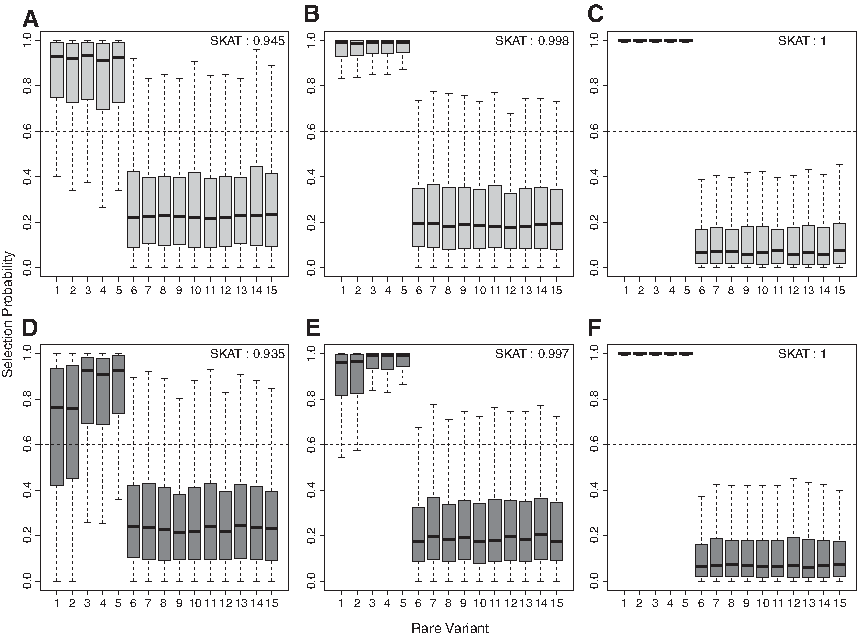
\end{document}. In terms of a logistic regression, odds ratio is around 2.71, so it can be regarded as a moderate effect size. For each variant-mix scenario and sample size, selection probabilities of 15 rare variants were computed over 1000 times. The box plots of selection probabilities are displayed in Figure 1.
The box plots of selection probabilities of risk (R), protective (P), and noncausal (N) rare variants are presented based on 1000 simulation replications when the variant effect size is moderate \documentclass{aastex}\usepackage{amsbsy}\usepackage{amsfonts}\usepackage{amssymb}\usepackage{bm}\usepackage{mathrsfs}\usepackage{pifont}\usepackage{stmaryrd}\usepackage{textcomp}\usepackage{portland, xspace}\usepackage{amsmath, amsxtra}\usepackage{upgreek}\pagestyle{empty}\DeclareMathSizes{10}{9}{7}{6}\begin{document}
$$( \gamma = 0.4 )$$
\end{document}. The sample size is 1000 for (A, D), 2000 for (B, E), and 5000 for (C, F). There are 5R/0P/10N variants in (A–C) and 3R/2P/10N variants in (D–F).
In Figure 1, the SKAT power is included at the top right of each plot. It represents the proportion of simulation replications, where the p value of SKAT was less than 0.05, among 1000 simulations. Selection probabilities were computed only when the SKAT rejected the null hypothesis of no association between 15 rare variants and the outcome. Three plots in the upper row are for the first variant-mix scenario (5R/0P/10N) and other three plots in the lower row are for the second variant-mix scenario (3R/2P/10N). Three columns represent three different sample sizes of 1000, 2000, and 5000, respectively. Overall, we can see that both risk and protective variants are well separated from noncausal variants. In other words, selection probabilities of both risk and protective variants are indeed much higher than those of noncausal variants. When the sample size is 5000, selection probabilities of risk and protective variants are almost 1. It seems that the variance of selection probabilities is overall increased for smaller sample size as expected. When both risk and protective variants are present in the same gene such as the second variant-mix scenario, the aPset method prescreens potentially protective variants through a marginal association test. But, the marginal test to detect protective variants is likely to be underpowered when either the sample size or the variant effect size is relatively small. This limitation of the aPset method is also discussed in Sun and Wang (2014). As we applied the aPset method to compute selection probabilities, the selection probabilities of protective variants seem to have higher variances than those of other variants when the sample size is 1000. But, this difference becomes negligible as the sample size increases.
3.2. Performance of new selection approach
In the second simulation study, we compared the selection performance of the proposed new selection approach using the threshold \documentclass{aastex}\usepackage{amsbsy}\usepackage{amsfonts}\usepackage{amssymb}\usepackage{bm}\usepackage{mathrsfs}\usepackage{pifont}\usepackage{stmaryrd}\usepackage{textcomp}\usepackage{portland, xspace}\usepackage{amsmath, amsxtra}\usepackage{upgreek}\pagestyle{empty}\DeclareMathSizes{10}{9}{7}{6}\begin{document}
$$\alpha = 0.6$$
\end{document} of selection probability with that of aPset. In addition to the aPset method, we also considered the weighted aPset (wPset) method, which is essentially the same as aPset except that it has individual variant weights \documentclass{aastex}\usepackage{amsbsy}\usepackage{amsfonts}\usepackage{amssymb}\usepackage{bm}\usepackage{mathrsfs}\usepackage{pifont}\usepackage{stmaryrd}\usepackage{textcomp}\usepackage{portland, xspace}\usepackage{amsmath, amsxtra}\usepackage{upgreek}\pagestyle{empty}\DeclareMathSizes{10}{9}{7}{6}\begin{document}
$${ \omega _j}$$
\end{document} in Equation (1) for \documentclass{aastex}\usepackage{amsbsy}\usepackage{amsfonts}\usepackage{amssymb}\usepackage{bm}\usepackage{mathrsfs}\usepackage{pifont}\usepackage{stmaryrd}\usepackage{textcomp}\usepackage{portland, xspace}\usepackage{amsmath, amsxtra}\usepackage{upgreek}\pagestyle{empty}\DeclareMathSizes{10}{9}{7}{6}\begin{document}
$$j = 1 , \ldots , p$$
\end{document}. One of the most popular weights for rare variants is an inverse of standard deviations of the estimated MAF, which has been proposed by Madsen and Browning (2009). It has been already demonstrated that wPset can perform more powerful selection than aPset in case–control association studies (Sun and Wang, 2014; Kim et al., 2015). In Figure 1, we can see that the threshold of 0.6 can roughly separate both risk and protective variants from noncausal variants. We denoted two proposed selection approaches using the threshold of 0.6 by aPset0.6 and wPset0.6. The former is based on selection probabilities of the aPset method, whereas the later is based on selection probabilities of the wPset method.
Similar to Sun and Wang (2014) and Kim et al. (2015), we computed two quantities such as ASP and selection power to compare selection performance of four methods: aPset, aPset0.6, wPset, and wPset0.6. The ASP of risk variants is defined as
\documentclass{aastex}\usepackage{amsbsy}\usepackage{amsfonts}\usepackage{amssymb}\usepackage{bm}\usepackage{mathrsfs}\usepackage{pifont}\usepackage{stmaryrd}\usepackage{textcomp}\usepackage{portland, xspace}\usepackage{amsmath, amsxtra}\usepackage{upgreek}\pagestyle{empty}\DeclareMathSizes{10}{9}{7}{6}\begin{document}
\begin{align*}
{ \rm { ASP \ of \ risk \ variants } } = \frac { R } { { K { R_0 } } } ,
\end{align*}
\end{document}
where K = 1000 is the number of simulation replications, R is the number of selected risk variants among K simulations, and R0 is the total number of true risk variants so R0 = 5 for the first variant-mix scenario and R0 = 3 for the second variant-mix scenario. Similarly, the ASP of protective and noncausal variants can be defined. The larger the ASP of causal (risk and protective) variants and the smaller the ASP of noncausal variants, the better the selection performance. The selection power of each method is defined as the simulation proportion that each method selects exactly all of the causal (both risk and protective) variants among K simulations (Sun and Wang, 2014; Kim et al., 2015). As computing selection power of each method, we only counted simulation replications where the exact five causal variants were selected in both variant-mix scenarios.
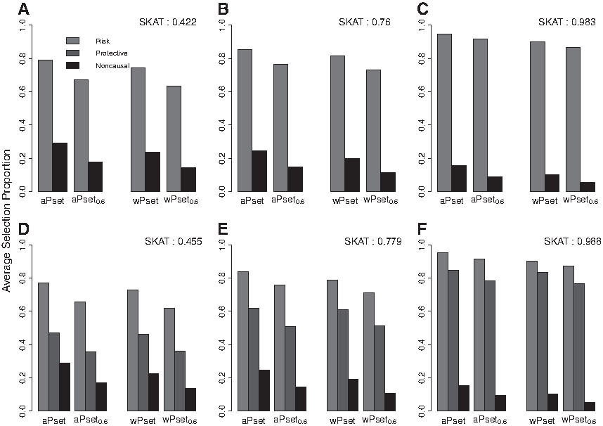
Figure 2 shows ASP of the four methods for each of three different sample sizes (by columns) and two different variant-mix scenarios (by rows) used in the first simulation study. But, in this simulation we set \documentclass{aastex}\usepackage{amsbsy}\usepackage{amsfonts}\usepackage{amssymb}\usepackage{bm}\usepackage{mathrsfs}\usepackage{pifont}\usepackage{stmaryrd}\usepackage{textcomp}\usepackage{portland, xspace}\usepackage{amsmath, amsxtra}\usepackage{upgreek}\pagestyle{empty}\DeclareMathSizes{10}{9}{7}{6}\begin{document}
$$\gamma = 0.2$$
\end{document} so that the average variant effect size is around 0.5, that is, \documentclass{aastex}\usepackage{amsbsy}\usepackage{amsfonts}\usepackage{amssymb}\usepackage{bm}\usepackage{mathrsfs}\usepackage{pifont}\usepackage{stmaryrd}\usepackage{textcomp}\usepackage{portland, xspace}\usepackage{amsmath, amsxtra}\usepackage{upgreek}\pagestyle{empty}\DeclareMathSizes{10}{9}{7}{6}\begin{document}
$${ \rm{avg}} ( \vert { \beta _j} \vert ) = 0.5$$
\end{document}. In terms of a logistic regression, odds ratio is around 1.65, so it can be regarded as a small effect size. We can see that SKAT power was noticeably decreased compared with the power in the first simulation because the variant effect size was actually decreased. As shown in Figure 2, all ASPs of the proposed selection approach (aPset0.6 and wPset0.6) are slightly lower than ASPs of aPset and wPset, respectively. In other words, both aPset0.6 and wPset0.6 reduced false positives (noncausal variants) while they decreased true positives (risk and protective variants) at the same time. In this simulation result, we can conclude that the proposed selection approach is flexible in terms of variant selection. When smaller model selection is desired to avoid false positives, we just need to increase the threshold α more than 0.6. In contrast, when larger model selection is desired to have more true positives, we just need to decrease the threshold α less than 0.6. However, aPset and wPset methods cannot control true and false positives because their selection results are summarized as just selected or not selected.
Averaged selection proportions of risk (R), protective (P), and noncausal (N) rare variants for aPset (data-adaptive power set-based selection), aPset0.6 (selection using selection probability of aPset with a threshold of 0.6), wPset (weighted aPset), and wPset0.6 (weighted aPset0.6) methods are displayed when the variant effect size is small \documentclass{aastex}\usepackage{amsbsy}\usepackage{amsfonts}\usepackage{amssymb}\usepackage{bm}\usepackage{mathrsfs}\usepackage{pifont}\usepackage{stmaryrd}\usepackage{textcomp}\usepackage{portland, xspace}\usepackage{amsmath, amsxtra}\usepackage{upgreek}\pagestyle{empty}\DeclareMathSizes{10}{9}{7}{6}\begin{document}
$$( \gamma = 0.2 )$$
\end{document}. The sample size is 1000 for (A, D), 2000 for (B, E), and 5000 for (C, F). There are 5R/0P/10N variants in (A–C) and 3R/2P/10N variants in (D–F).
Next, we compared selection power of four selection methods along with different variant effect sizes, where the variant effect size was set from \documentclass{aastex}\usepackage{amsbsy}\usepackage{amsfonts}\usepackage{amssymb}\usepackage{bm}\usepackage{mathrsfs}\usepackage{pifont}\usepackage{stmaryrd}\usepackage{textcomp}\usepackage{portland, xspace}\usepackage{amsmath, amsxtra}\usepackage{upgreek}\pagestyle{empty}\DeclareMathSizes{10}{9}{7}{6}\begin{document}
$$\gamma = 0.2$$
\end{document} to \documentclass{aastex}\usepackage{amsbsy}\usepackage{amsfonts}\usepackage{amssymb}\usepackage{bm}\usepackage{mathrsfs}\usepackage{pifont}\usepackage{stmaryrd}\usepackage{textcomp}\usepackage{portland, xspace}\usepackage{amsmath, amsxtra}\usepackage{upgreek}\pagestyle{empty}\DeclareMathSizes{10}{9}{7}{6}\begin{document}
$$\gamma = 0.7$$
\end{document}, increased by 0.1. Correspondingly, the odds ratio increases from around 1.65 to 5.75. Figure 3 shows selection powers of the four methods for each of three different sample sizes (by columns) and two different variant-mix scenarios (by rows) used in the first simulation study. First, it is noticeable that selection power of aPset0.6 is much higher than that of aPset in all of six plots. However, selection power of wPset0.6 is slightly higher than that of wPset when the sample size is small. The wPset method shows the best selection power when the sample size is large enough. The powerful selection performance of wPset has also been demonstrated by Sun and Wang (2014) and Kim et al. (2015). We compared ASP and selection power of the proposed selection approach with the existing methods only when the threshold \documentclass{aastex}\usepackage{amsbsy}\usepackage{amsfonts}\usepackage{amssymb}\usepackage{bm}\usepackage{mathrsfs}\usepackage{pifont}\usepackage{stmaryrd}\usepackage{textcomp}\usepackage{portland, xspace}\usepackage{amsmath, amsxtra}\usepackage{upgreek}\pagestyle{empty}\DeclareMathSizes{10}{9}{7}{6}\begin{document}
$$\alpha = 0.6$$
\end{document}. In the next simulation study, we considered a different value of α.
Selection powers of aPset (data-adaptive power set-based selection), aPset0.6 (selection using selection probability of aPset with a threshold of 0.6), wPset (weighted aPset), and wPset0.6 (weighted aPset0.6) methods are displayed along with different variant effect sizes. The sample size is 1000 for (A, D), 2000 for (B, E), and 5000 for (C, F). There are 5 risk and 10 noncausal variants in (A–C) and 3 risk, 2 protective, and 10 noncausal variants in (D–F).
3.3. Optimal threshold of selection probability
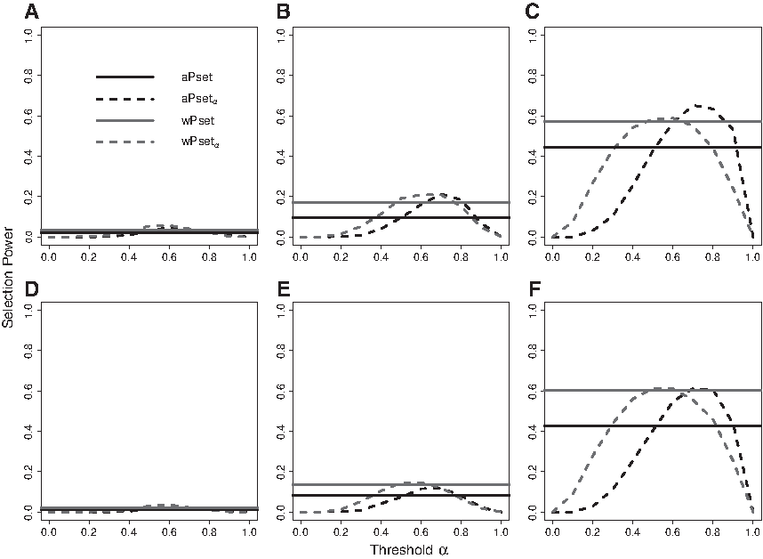
In this simulation, we additionally investigated selection power of the proposed selection approach along with a different value of \documentclass{aastex}\usepackage{amsbsy}\usepackage{amsfonts}\usepackage{amssymb}\usepackage{bm}\usepackage{mathrsfs}\usepackage{pifont}\usepackage{stmaryrd}\usepackage{textcomp}\usepackage{portland, xspace}\usepackage{amsmath, amsxtra}\usepackage{upgreek}\pagestyle{empty}\DeclareMathSizes{10}{9}{7}{6}\begin{document}
$$\alpha \in [ 0 , 1 ]$$
\end{document}. Figure 4 shows selection powers of aPsetα and wPsetα along with a different threshold for each of three different sample sizes (by columns) and two different variant-mix scenarios (by rows) used in the first simulation study. In this simulation, we fixed the variant effect size as \documentclass{aastex}\usepackage{amsbsy}\usepackage{amsfonts}\usepackage{amssymb}\usepackage{bm}\usepackage{mathrsfs}\usepackage{pifont}\usepackage{stmaryrd}\usepackage{textcomp}\usepackage{portland, xspace}\usepackage{amsmath, amsxtra}\usepackage{upgreek}\pagestyle{empty}\DeclareMathSizes{10}{9}{7}{6}\begin{document}
$$\gamma = 0.3$$
\end{document}, and two reference lines of the selection powers of both aPset and wPset were added for comparison. First of all, we can see that the optimal α of aPsetα and wPsetα that can maximize selection power is different from each other. For example, the optimal α of aPsetα should be greater than 0.6 when the sample size is 5000. But, the optimal α of aPsetα should be less than 0.6 when the sample size is 5000. Also, the optimal α value seems to be slightly different when the sample size is smaller. Although we did not include other simulation results about the optimal α when the variant effect size is different from \documentclass{aastex}\usepackage{amsbsy}\usepackage{amsfonts}\usepackage{amssymb}\usepackage{bm}\usepackage{mathrsfs}\usepackage{pifont}\usepackage{stmaryrd}\usepackage{textcomp}\usepackage{portland, xspace}\usepackage{amsmath, amsxtra}\usepackage{upgreek}\pagestyle{empty}\DeclareMathSizes{10}{9}{7}{6}\begin{document}
$$\gamma = 0.3$$
\end{document}, we confirmed that the optimal α also varies on different variant effect sizes. Based on our extensive simulation studies, our new selection approach with \documentclass{aastex}\usepackage{amsbsy}\usepackage{amsfonts}\usepackage{amssymb}\usepackage{bm}\usepackage{mathrsfs}\usepackage{pifont}\usepackage{stmaryrd}\usepackage{textcomp}\usepackage{portland, xspace}\usepackage{amsmath, amsxtra}\usepackage{upgreek}\pagestyle{empty}\DeclareMathSizes{10}{9}{7}{6}\begin{document}
$$\alpha = 0.6$$
\end{document} has overall shown relatively strong selection performance in most of simulation settings.
Selection powers of aPsetα (selection using selection probability of aPset with a threshold of α) and wPsetα (weighted aPsetα) methods are displayed along with different values of threshold α when the variant effect size is small \documentclass{aastex}\usepackage{amsbsy}\usepackage{amsfonts}\usepackage{amssymb}\usepackage{bm}\usepackage{mathrsfs}\usepackage{pifont}\usepackage{stmaryrd}\usepackage{textcomp}\usepackage{portland, xspace}\usepackage{amsmath, amsxtra}\usepackage{upgreek}\pagestyle{empty}\DeclareMathSizes{10}{9}{7}{6}\begin{document}
$$( \gamma = 0.3 )$$
\end{document}. Two reference lines of selection powers of aPset (data-adaptive power set-based selection) and wPset (weighted aPset) are included for comparison. The sample size is 1000 for (A, D), 2000 for (B, E), and 5000 for (C, F). There are 5 risk and 10 noncausal variants in (A–C) and 3 risk, 2 protective, and 10 noncausal variants in (D–F).
4. Real Sequencing Data Analysis
We applied the four selection methods (aPset, wPset, aPset0.6, wPset0.6) discussed in the simulation studies to the DHS data (Romeo et al., 2007, 2009). The DHS data include four genes ANGPTL3, ANGPTL4, ANGPTL5, and ANGPTL6 with nine energy metabolism traits, namely triglyceride (TG), low-density lipoprotein (LDL), very LDL (VLDL), high-density lipoprotein, cholesterol, glucose, body mass index, systolic blood pressure (SBP), and diastolic blood pressure. Association studies between each trait and each of four genes have been conducted in many different studies (Liu and Leal, 2010, 2012; Price et al., 2010; Wu et al., 2011; Yi et al., 2011; Cheung et al., 2012). All of these studies performed a gene-based group association test so they could only identify the association between one of four genes and one of nine traits. They have commonly identified the association of the gene ANGPTL4 with both traits VLDL and TG for the European American population, and the association of the gene ANGPTL5 with the trait SBP for Hispanic population. Recently, additional investigation to locate risk and protective variants within the genes ANGPTL4 and ANGPTL5 has been performed by Sun and Wang (2014), where the aPset and wPset methods were applied to multiple rare variants within the genes ANGPTL4 and ANGPTL5. As we pointed out earlier, these methods can be summarized as only either selected variants or unselected variants. Therefore, the certainty of selected and unselected variants could not be measured by the existing methods. Instead, we computed selection probabilities of individual variants to quantify the certainty of both selected and unselected variants.
In Table 1, the selection results of the ANGPTL4 gene associated with the trait TG for the European American population are present along with selection probabilities of aPset and wPset. It is noticeable that selection probabilities of selected variants are quite different, so we can compare selected variants in terms of the strength of association. For example, we can be very confident with the variant X1313_E40K for association with TG because the selection probabilities of both aPset and wPset are more than 0.95, whereas the selection probabilities of the variants X6113_E190Q and X8020_P251T, which were selected by aPset, are a boundary of 0.6 for aPset but much less than for wPset. Further investigation on these two variants might be necessary to see whether they are potentially false positives.
Rare Variant Selection Result of the ANGPTL4 Gene Associated with the Trait Triglyceride
Variants
aPset
SP
aPset0.6
wPset
SP
wPset0.6
X1313_E40K
X
0.966
X
X
0.954
X
X3145_E167K
0.102
0.106
X6113_E190Q
X
0.610
X
0.267
X7936_G223R
0.092
0.090
X8003_K245fs
0.107
0.102
X8020_P251T
X
0.600
0.269
X8262_S302fs
0.084
0.083
X8364_R336C
0.327
0.327
X10621_G361S
0.098
0.081
SP, a selection probability; X, a selected variant.
As given in Table 2, the selection results of the ANGPTL4 gene associated with the trait VLDL for European American population are present along with selection probabilities of aPset and wPset. Similarly, we can conclude that the variant X1313_E40K has a strong association with the VLDL. In contrast, the three variants X6113_E190Q, X8003_K245fs, and X8020_P251T have relatively small selection probabilities, although aPset, aPset0.6, and wPset located all of these three variants. Also, we can see that the unselected variant X8364_R336C has relatively high selection probability compared with other unselected variants. This variant could be truly noncausal, but it has higher chance to be a false negative than other unselected variants.
Rare Variant Selection Result of the ANGPTL4 Gene Associated with the Trait Very Low-Density Lipoprotein
Variants
aPset
SP
aPset0.6
wPset
SP
wPset0.6
X1313_E40K
X
0.962
X
X
0.955
X
X3145_E167K
0.071
0.072
X6113_E190Q
X
0.614
X
X
0.456
X7936_G223R
0.063
0.075
X8003_K245fs
X
0.618
X
X
0.578
X8020_P251T
X
0.617
X
X
0.446
X8262_S302fs
0.078
0.063
X8364_R336C
0.486
0.460
X10621_G361S
0.064
0.056
X, a selected variant.
Finally, the selection results of the ANGPTL5 gene associated with the trait SBP for Hispanic population are presented in Table 3. This table shows that aPset and wPset selected the same five variants, whereas aPset0.6 and wPset0.6 selected two of the five variants because only two variants are of relatively high selection probability. In our simulation studies, we have seen that ASPs of aPset0.6 and wPset0.6 are always lower than those of aPset and wPset, respectively. In our analysis with DHS data, all of three selection results are consistent with simulation selection results, where the selection method using the threshold of 0.6 is likely to select a smaller model than the aPset and wPset methods. This can lead to reduce false positives if unselected three variants were truly noncausal. However, the proposed selection could result in the loss of true positives if they were truly causal. Consequently, the proposed selection method using the threshold 0.6 seems to be more conservative than aPset and wPset.
Rare Variant Selection Result of the ANGPTL5 Gene Associated with the Trait Systolic Blood Pressure
Variants
aPset
SP
aPset0.6
wPset
SP
wPset0.6
S93N
X
0.788
X
X
0.743
X
L98P
X
0.572
X
0.580
L125F
0.175
0.192
S175P
X
0.579
X
0.430
T268M
X
0.779
X
X
0.759
X
G309R
X
0.574
X
0.399
N329S
0.299
0.328
X, a selected variant.
5. Conclusion
In this article, we proposed selection probability of individual rare variants and a new selection approach based on a threshold of selection probabilities. The proposed selection probabilities can quantify the certainty of both selected and unselected rare variants, so that we can compare the strength of association signals among selected variants. Although there have been a few selection methods on rare variants, none of them were able to provide the certainty of their selection result. As the proposed selection probability is based on nonparametric bootstrap resampling, it can be applied to any of the existing selection methods. Moreover, the proposed selection approach using a threshold of selection probabilities has been demonstrated that it is not only flexible to control the size of selected variants but also powerful to select both risk and protective variants.
Although we could not suggest a method to pick up the optimal threshold of the proposed selection approach, we have shown that selection power of the proposed selection using the optimal threshold could be drastically increased, because the choice of the optimal threshold relies on many different factors such as a sample size, a gene size, a variant effect size, and the number of risk and protective variants. In addition to these factors, each rare variant has almost the same genotypes among the samples because the number of observed genetic mutations is extremely rare, so commonly used K-fold cross-validation to pick up the optimal threshold cannot be applied to rare variants. Development of a new idea to pick up the optimal threshold will be an interesting research topic in rare variants analysis.
Footnotes
Acknowledgments
This research was supported by Basic Science Research Program through the National Research Foundation of Korea (NRF) funded by the Ministry of Education (NRF-2016R1D1A1B03930218).
Author Disclosure Statement
The authors declare that no competing financial interests exist.
References
1.
AlexanderD., and LangeK.2011. Stability selection for genome-wide association. Genet. Epidemiol., 35, 722–728.
2.
CheungY., WangG., LealS., et al.2012. A fast and noise-resilient approach to detect rare-variant associations with deep sequencing data for complex disorders. Genet. Epidemiol., 36, 675–685.
3.
Ionita-LazaI., BuxbaumJ.D., LairdN.M., et al.2011. A new testing strategy to identify rare variants with either risk or protective effect on disease. PLoS Genet. 7, e1001289.
4.
Ionita-LazaI., CapanuM., De-RubeisS., et al.2014. Identification of rare causal variants in sequence-based studies: Methods and applications to VPS13B, a gene involved in Cohen syndrome and autism. PLoS Genet. 10, e1004729.
5.
Ionita-LazaI., LeeS., MakarovV., et al.2013. Sequence kernel association tests for the combined effect of rare and common variants. Am. J. Hum. Genet., 92, 841–853.
6.
KimS., LeeK., and SunH.2015. Statistical selection strategy for risk and protective rare variants associated with complex traits. J. Comput. Biol., 22, 1034–1043.
7.
LanderE.S.2011. Initial impact of the sequencing of the human genome. Nature, 470, 187–197.
8.
LeeS., AbecasisG., BoehnkeM., et al.2014. Rare-variant association analysis: Study designs and statistical tests. Am. J. Hum. Genet., 95, 5–23.
9.
LeeS., EmondM., BamshadM., et al.2012. Optimal unified approach for rare-variant association testing with application to small-sample case-control whole-exome sequencing studies. Am. J. Hum. Genet., 91, 224–237.
10.
LinD.-Y., and TangZ.-Z.2011. A general framework for detecting disease associations with rare variants in sequencing studies. Am. J. Hum. Genet., 89, 354–367.
11.
LiuD., and LealS.2010. A novel adaptive method for the analysis of next-generation sequencing data to detect complex trait associations with rare variants due to gene main effects and interactions. PLoS Genet. 6, e1001156.
12.
LiuD., and LealS.2012. Estimating genetic effects and quantifying missing heritabaility explained by identified rare-variant associations. Am. J. Hum. Genet., 91, 585–596.
13.
MadsenB.E., and BrowningS.R.2009. A groupwise association test for rare mutations using a weighted sum statistic. PLoS Genet. 5, e1000384.
14.
ManolioT., CollinsF., CoxN., et al.2009. Finding the missing heritability of complex diseases. Nature, 461, 747–753.
15.
MeinshausenN., and BühlmannP.2010. Stability selection. J. R. Stat. Soc. Series B, 72, 417–473.
16.
PriceA.L., KryukovG.V., de BakkerP.I., et al.2010. Pooled association tests for rare variants in exon-resequencing studies. Am. J. Hum. Genet., 86, 832–838.
17.
RomeoS., PennacchioL., FuY., et al.2007. Population-based resequencing of ANGPTL4 uncovers variations that reduce triglycerides and increase HDL. Nat. Genet., 39, 513–516.
18.
RomeoS., YinW., KozlitinaJ., et al.2009. Rare loss-of-function mutations in ANGPTL family members contribute to plasma triglyceride levels in humans. J. Clin. Invest., 119, 70–79.
19.
SunH., and WangS.2012. Penalized logistic regression for high-dimensional DNA methylation data analysis with case-control studies. Bioinformatics. 28, 1368–1375.
20.
SunH., and WangS.2013. Network-based regularization for matched case-control analysis of high-dimensional DNA methylation data. Stat. Med., 32, 2127–2139.
21.
SunH., and WangS.2014. A power set-based statistical selection procedure to locate susceptible rare variants associated with complex traits with sequencing data. Bioinformatics. 30, 2317–2323.
22.
SunJ., ZhengY., and HsuL.2013. A unified mixed-effects model for rare-variant association in sequencing studies. Genet. Epidemiol., 37, 3345–344.
23.
WuM.C., LeeS., CaiT., et al.2011. Rare-variant association testing for sequencing data with the sequence kernel association test. Am. J. Hum. Genet., 89, 82–93.
24.
YiN., LiuN., ZhiD., et al.2011. Hierarchical generalized linear models for multiple groups of rare and common variants: Jointly estimating group and individual-variant effects. PLoS Genet. 7, e1002382.
25.
ZukO., HechterE., SunyaevS.R., et al.2012. The mystery of missing heritability: Genetic interactions create phantom heritability. Proc. Natl. Acad. Sci., 109, 1193–1198.