GeNICE: A Novel Framework for Gene Network Inference by Clustering,Exhaustive Search,and Multivariate Analysis

Abstract

Gene network (GN) inference from temporal gene expression data is a crucial and challenging problem in systems biology. Expression data sets usually consist of dozens of temporal samples, while networks consist of thousands of genes, thus rendering many inference methods unfeasible in practice. To improve the scalability of GN inference methods, we propose a novel framework called GeNICE, based on probabilistic GNs; the main novelty is the introduction of a clustering procedure to group genes with related expression profiles and to provide an approximate solution with reduced computational complexity. We use the defined clusters to perform an exhaustive search to retrieve the best predictor gene subsets for each target gene, according to multivariate criterion functions. GeNICE greatly reduces the search space because predictor candidates are restricted to one gene per cluster. Finally, a multivariate analysis is performed for each defined predictor subset to retrieve minimal subsets and to simplify the network. In our experiments with in silico generated data sets, GeNICE achieved substantial computational time reduction when compared to solutions without the clustering step, while preserving the gene expression prediction accuracy even when the number of clusters is small (about 50) relative to the number of genes (order of thousands). For a Plasmodium falciparum microarray data set, the prediction accuracy achieved by GeNICE was roughly 97%, while the respective topologies involving glycolytic and apicoplast seed genes had a very large intramodularity, very small interconnection between modules, and some module hub genes, reflecting small-world and scale-free topological properties, as expected.

1. Introduction

A living organism is a complex biological system that can be interpreted as a network of molecules connected by chemical reactions and their regulatory mechanisms. Systems biology is a new scientific field that aims at the computational and mathematical modeling of such complex biological systems. Its purpose is to study the interactions between the components of biological systems and how these interactions give rise to the function and behavior of that system. In fact, one of the major goals of systems biology is to reveal how genes and their products interact for regulation of cellular processes. Accomplishing this goal requires the reconstruction of gene regulatory networks (GRNs) (Pindah et al., 2015). Unsurprisingly, the modeling, inference, and interpretation of GRNs from temporal gene expression data have drawn significant attention (Hecker et al., 2009; Marbach et al., 2012; Shmulevich and Dougherty, 2014), particularly after the development of large-scale gene expression measurement techniques, such as cDNA microarrays (Shalon et al., 1996), SAGE (Velculescu et al., 1995), and more recently RNA-Seq (Wang et al., 2009).

The GRN inference problem involves the discovery of complex regulatory relationships among biological molecules that can describe diverse biological functions and also the dynamics of molecular activities. Once the network is recovered, intervention studies can be conducted to control the dynamics of biological systems aiming to prevent or treat diseases (Shmulevich and Dougherty, 2014). Genes and proteins usually form an intricate complex network where often the behavior of a given gene, measured by means of its expression level (i.e., mRNA abundance), depends on a multivariate and coordinated action of other genes and their by-products (proteins) (Martins et al., 2008). Thus, GRN inference based on gene expression data analysis requires robust methods and algorithms, and new approaches are constantly under evaluation. The importance of GRN reconstruction can also be seen through many initiatives, such as the project DREAM (Dialogue for Reverse Engineering Assessments and Methods) (Marbach et al., 2012).

There are two main approaches to gene interaction modeling (Shmulevich and Dougherty, 2014): the continuous one and the discrete one. A continuous approach considers mainly differential equations to obtain a quantitative detailed model of biochemical networks (De-Jong, 2002; Hecker et al., 2009). Although continuous models provide a detailed understanding of the system, they require prior information about the kinetic parameters and a large number of experimental samples (Hecker et al., 2009). On the contrary, discrete models measure the gene interactions from a qualitative point of view. Popular discrete models include those based on graphs such as Bayesian networks (Friedman et al., 2000), Boolean networks (BNs) (Kauffman, 1969), and their stochastic versions, probabilistic Boolean networks (PBN) (Shmulevich et al., 2002) and probabilistic gene networks (PGNs), a PBN model with some constraints (Barrera et al., 2007). Discrete models can capture the overall behavior of system dynamics, requiring less data to be built and being easier to implement and analyze (Hecker et al., 2009). Discrete modeling has been successfully used in analysis and simulation of a myriad of biological networks, such as those for Drosophila melanogaster (Sánchez and Thieffry, 2001; Albert and Othmer, 2003), yeast cell cycle (Li et al., 2004; Zhang et al., 2006; Davidich and Bornholdt, 2008), Arabidopsis thaliana (Espinosa-Soto et al., 2004), mammal cell cycle (Faure et al., 2006), and Plasmodium falciparum (Barrera et al., 2007).

GRN inference is an ill-posed problem: for a given data set of gene expression profiles, there are many (if not infinite) networks capable of generating the same data set. This problem is further hampered due to the typically limited number of samples, the huge dimensionality (number of variables, i.e., genes), and the presence of noise (Hecker et al., 2009; Shmulevich and Dougherty, 2014). There is a vast literature dealing with the GRN inference problem (Bansal et al., 2007; Markowetz and Spang, 2007; Hecker et al., 2009; De-Smet and Marchal, 2010; Marbach et al., 2012). Some examples of methods that deal with this problem include entropy-based feature selection (Liang et al., 1998; Lopes et al., 2014), relevance networks (Margolin et al., 2006; Faith et al., 2007), feature selection by maximum relevance/minimum redundancy (Meyer et al., 2007; Hira and Gillies, 2015), and signal perturbation (Ideker et al., 2000; Carastan-Santos et al., 2017), among others.

In the specific context of discrete models, BNs and PBNs can generalize and capture the global behavior of biological systems (Kauffman, 1969; Shmulevich et al., 2002). These models are appropriate in experimental settings where the number of experiments is on the order of dozens and the dimensionality is on the order of thousands, as is the case of gene expression data experiments. The main disadvantage of these models is information loss as a consequence of the required data quantization. However, quantization makes BN and PBN models simpler to implement and analyze (Styczynski and Stephanopoulos, 2005; Ivanov and Dougherty, 2006), and many methods have been proposed to model GRNs through BNs or PBNs (Liang et al., 1998; Akutsu et al., 1999; Lahdesmaki and Shmulevich, 2003; Nam et al., 2006).

Although PBN genes have only two possible expression values, network inferences are still difficult, because the curse of dimensionality still shows its ugly head. Hence, the PGN model simplifies the inference process by local feature selection, to search for the best subsets of genes to predict the behavior of a given target gene (Barrera et al., 2007). Because exhaustive search is the only feature selection algorithm that guarantees optimality (Cover and van Campenhout, 1977), high-performance computing techniques are required when using this algorithm to search for predictor subsets of three or four dimensions (for larger dimensions, this technique is impractical) (Borelli et al., 2013; Carastan-Santos et al., 2017). An alternative to reducing the computational complexity of the exhaustive search is to apply some prior dimensionality reduction technique to restrict the search space of candidate predictor subsets for a given target. However, this is not trivial, as features that are weak individually may be strong in predicting a particular target when combined with others. Likewise, the best individual characteristics might not be as good at predicting the target when combined with others (Pudil et al., 1994; Martins et al., 2008).

In this article, we contribute with a new GRN inference framework for PGNs, called GeNICE (Gene Network Inference by Clustering, Exhaustive search, and multivariate analysis). This framework alleviates the inherent dimensionality curse of the GRN inference problem and, consequently, its computational cost. Our contribution is centered on the application of clustering techniques to reduce the search complexity when evaluating all possible predictor subsets, and thus to alleviate the computational complexity of the GRN inference. GeNICE performs a local feature selection for each target gene to obtain the best subsets of predictors given by the cluster representative genes. Besides, an intrinsically multivariate analysis is conducted to eliminate redundant features from each predictor subset (Martins et al., 2008) and, consequently, to obtain a minimal network.

Experimental results adopting data generated by SysGenSIM (Pinna et al., 2011), used by the DREAM 5 challenge (Marbach et al., 2012), show that the expression profiles (dynamics) produced by the minimum classification error logic of the selected predictor subsets with regard to the target are usually very close to the original expression profiles of the target cluster genes (about 90% of identity). Besides, experiments using P. falciparum (a malaria agent) temporal microarray data achieved even higher accuracies (97% in average). Regarding this same malaria data set, a topological analysis was conducted, displaying connected components for glycolysis and apicoplast functions with only one predictor subset for each target gene seed. Besides, the retrieved topological structure around the considered seeds displayed small-world and scale-free properties, which are commonly seen in biological networks (Strogatz, 2001; Barabási and Oltvai, 2004). In fact, the method displayed great computational efficiency on inferring networks and, at the same time, such networks produced better expression profiles and topologies than those generated by the networks inferred by the same process without involving clustering and multivariate analysis for removal of redundant features as initial and final steps, respectively.

2. Methods

In this study, we propose a new framework for GRN inference, named GeNICE (Gene Network Inference by Clustering, Exhaustive search, and multivariate analysis). GeNICE follows the PGN model (Barrera et al., 2007), which assumes that the temporal gene expression samples follow a first-order Markov chain where each target gene in a given time point depends only on its predictor subset values in the previous time instant. In addition, the transition function of the PGN model is homogeneous (it does not change over time), almost deterministic (from any state, the system has a preferential state to go), and conditionally independent (i.e., the expression value of a given gene is dependent only on its predictors, following the Markov hypothesis). These assumptions are important simplifications to deal with the limited number of samples typically available in real gene expression data. Fig. 1 shows the general workflow of GeNICE, the modules of which are described in the following.

FIG. 1.

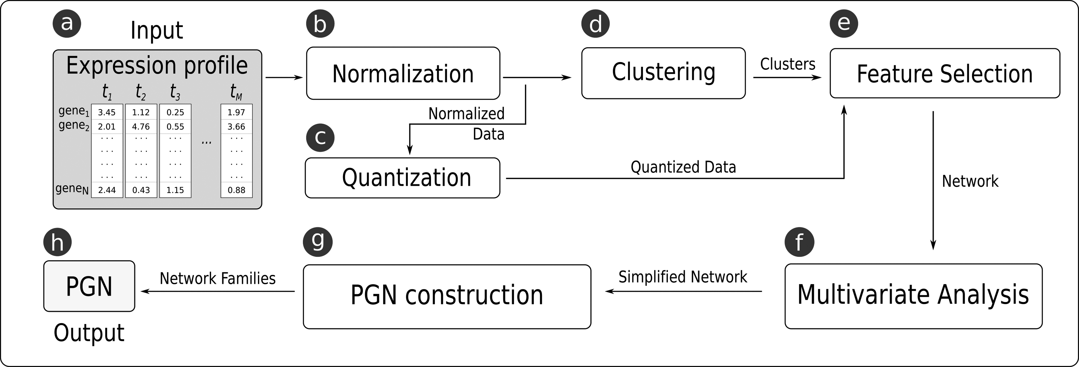
The main steps performed by GeNICE to infer gene networks following the PGN model. The box (a) represents the gene expression profiles as input, and the box (h) represents the final PGN as output. PGN, probabilistic gene networks.

2.1. Gene expression data

GeNICE starts with a gene expression time series data set as input (Fig. 1a) that consists of an N × M matrix showing the expression levels of the N genes at M consecutive time points (see Fig. 2a for an example).

FIG. 2.

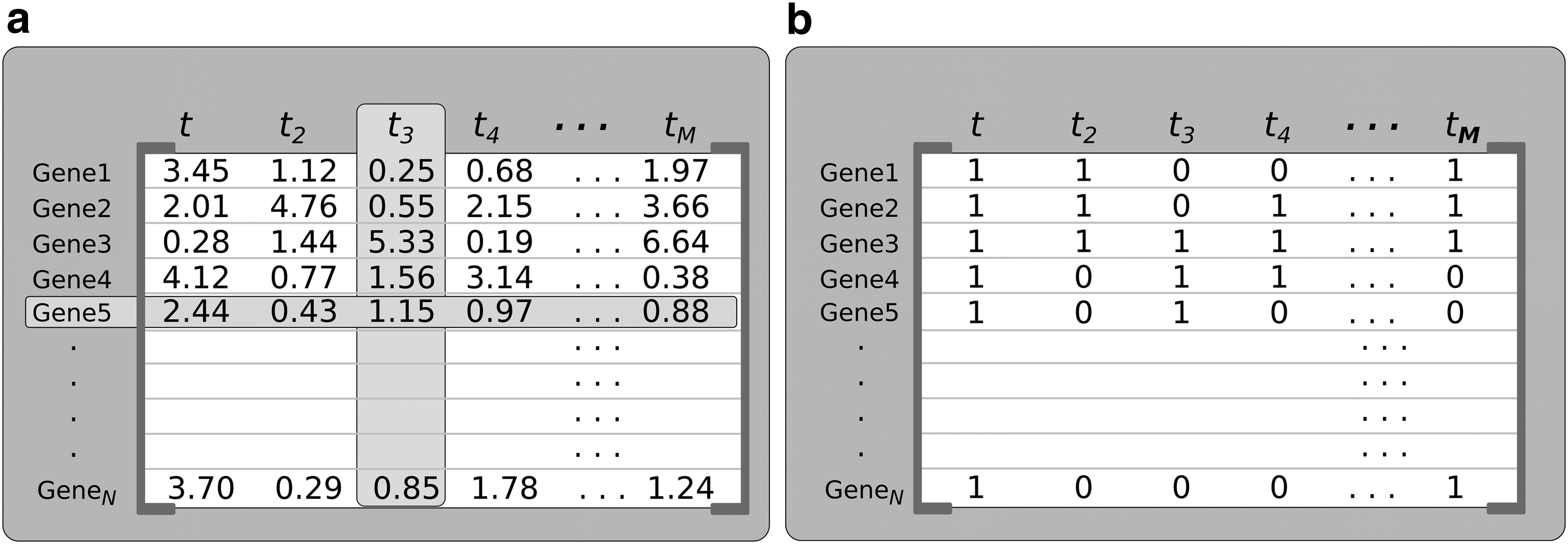
Example of a set of gene expression data: (a) the original matrix: rows are genes and columns are time points; (b) a binary gene expression profile.

2.2. Normalization

The data come from different experiments performed at each time point or may have fluctuations and noises in relation to the expression of each gene; so, a normalization operation (Fig. 1b) is required for the data to be comparable. A usual normalization procedure, which we adopt in GeNICE, is the normal transform or Z-score that transforms the data in such a way that each gene expression profile has zero mean and unitary standard deviation (Azuaje and Dopazo, 2005). Thus, the expression e_i of a given gene i becomes \documentclass{aastex}\usepackage{amsbsy}\usepackage{amsfonts}\usepackage{amssymb}\usepackage{bm}\usepackage{mathrsfs}\usepackage{pifont}\usepackage{stmaryrd}\usepackage{textcomp}\usepackage{portland, xspace}\usepackage{amsmath, amsxtra}\usepackage{upgreek}\pagestyle{empty}\DeclareMathSizes{10}{9}{7}{6}\begin{document} $${e^{\prime}_i} = ( {e_i} - { \mu _i} ) / { \sigma _i}$$ \end{document} , where \documentclass{aastex}\usepackage{amsbsy}\usepackage{amsfonts}\usepackage{amssymb}\usepackage{bm}\usepackage{mathrsfs}\usepackage{pifont}\usepackage{stmaryrd}\usepackage{textcomp}\usepackage{portland, xspace}\usepackage{amsmath, amsxtra}\usepackage{upgreek}\pagestyle{empty}\DeclareMathSizes{10}{9}{7}{6}\begin{document} $${ \mu _i}$$ \end{document} and \documentclass{aastex}\usepackage{amsbsy}\usepackage{amsfonts}\usepackage{amssymb}\usepackage{bm}\usepackage{mathrsfs}\usepackage{pifont}\usepackage{stmaryrd}\usepackage{textcomp}\usepackage{portland, xspace}\usepackage{amsmath, amsxtra}\usepackage{upgreek}\pagestyle{empty}\DeclareMathSizes{10}{9}{7}{6}\begin{document} $${ \sigma _i}$$ \end{document} are average and standard deviation of the expressions of gene i, respectively. This transformation aims at changing the data in such a way that expression values of a given gene below its own average become negative (underexpressed), while expressions above its own average become positive (overexpressed) (Cheadle et al., 2003). This characteristic is important because it preserves the shape of the gene profile.

2.3. Quantization

Since GeNICE follows the PGN model, the gene expression data set must be quantized (Fig. 1c) so that each gene expression presents a finite set of possible values. In this study, we adopt the binary quantization where negative Z-scored values become 0, while positive Z-scored values become 1. An example of the result of this step can be seen in Fig. 2b.

2.4. Clustering

Gene expression data can be clustered based on genes, samples, or both at the same time (biclustering, coclustering, block clustering, or two-mode clustering) (Govaert and Nadif, 2013). Each clustering type has specific applications and presents specific challenges for the clustering task.

GeNICE focuses on gene clustering (Fig. 1d). The clustering step preceding feature selection is one of the novelties. This step is important to reduce the dimensionality of possible candidate gene predictors for each gene target (in the order of thousands) to the order of the number of resulting clusters k (ideally in the order of dozens). This can have a great impact in the feature selection process (see Section 2.5), since the number of clusters (k) becomes the resulting dimensionality of the feature selection inference process, which could drastically reduce the number of calculated criterion functions depending on the chosen feature selection algorithm.

After normalization, the time series data are clustered by grouping genes with similar normalized real-value expression profiles. Any clustering technique that returns a partition and a list of members per cluster, including their respective representative genes, can be used. Self-organizing map, k-means, hierarchical approaches, Fuzzy C-means, and others display very different results in some cases (Hu and Yoo, 2004). One of the most popular clustering techniques is the k-means algorithm. It partitions N observations (genes) into k clusters, in which each observation belongs to the cluster with the nearest mean value across the time points.

The k-means algorithm starts with k initial centroid values from randomly selected samples and then proceeds in two alternate steps: (1) an allocation step, where all samples are allocated to the cluster containing the centroid that yields the least within-cluster sum of squares (usually the squared Euclidean distance) and (2) a representation step, where a new centroid is constructed for each cluster, that is, new means are calculated to be the centroids of the samples in the new clusters (Pindah et al., 2015).

GeNICE uses a variant of this algorithm that initializes the k centroid values with a predefined set of points selected from the input data and adopts two within-cluster distance measures: Euclidean distance and absolute Pearson correlation. The distance measure chosen is very important because it defines different types of similarity among gene profiles. For instance, Fig. 3a and b represents gene expression signals belonging to the same cluster according to Euclidean distance and absolute Pearson correlation, respectively. In particular, clustering by absolute Pearson correlation tends to group genes whose expression profiles present both similar and opposite phase shapes in the same cluster. This criterion is more desirable than regular Pearson correlation or Euclidean distance for the specific purpose of deriving the best predictors for a given target gene, since strongly correlated candidate predictors (positive or negative) are redundant to each other. Thus, genes with strong negative correlation that compose the same cluster cannot participate in the same predictor subset for a given target, since only one representative gene for each cluster is admitted (and only this representative gene can be a candidate predictor in GeNICE).

FIG. 3.

Clustering gene expression profiles with the same relative patterns (Azuaje and Dopazo, 2005): (a) Euclidean Distance; (b) absolute Pearson correlation.

At the end of the clustering step, one representative gene from each cluster must be defined. These genes compose the set of candidate predictors \documentclass{aastex}\usepackage{amsbsy}\usepackage{amsfonts}\usepackage{amssymb}\usepackage{bm}\usepackage{mathrsfs}\usepackage{pifont}\usepackage{stmaryrd}\usepackage{textcomp}\usepackage{portland, xspace}\usepackage{amsmath, amsxtra}\usepackage{upgreek}\pagestyle{empty}\DeclareMathSizes{10}{9}{7}{6}\begin{document} $${ \bf{C}} = \{ {C_1} , {C_2} , \ldots , {C_k} \} \subseteq { \bf{X}}$$ \end{document} considered in the feature selection step, where X is the set of genes (with cardinality N), C is the set of candidate predictors (with cardinality k), and C_i is a representative gene of the cluster i. When using Euclidean distance, the representative gene of a given cluster is the one with the smallest Euclidean distance to the centroid (average of gene expression signals) (Liao, 2005; Achtert et al., 2010). In its turn, for absolute Pearson correlation, the representative gene of a given cluster is the one with the largest mean of absolute Pearson correlations between its expression profile and all other gene expression profiles in the same cluster.

2.5. Feature selection

Feature selection is a crucial step in the PGN inference procedure. A feature selection problem consists in selecting a subset of features that best represents the objects under study. In the PGN inference context, a feature selection algorithm consists basically in searching for subsets of genes that best predict a given target gene according to a criterion function, which assigns a quality value for a candidate predictor subset according to its expression profiles and the target expression profile (Barrera et al., 2007, Borelli et al., 2013, Lopes et al., 2014).

In GeNICE, the feature selection algorithm is applied considering each target gene, aiming to achieve the best predictor subset for that target, according to a given criterion function. All representative genes (one gene per cluster achieved in the clustering step) are taken as potential predictor genes, and hence, all other genes are ignored.

There are many feature selection algorithms proposed in the literature, most of them are computationally efficient but suboptimal. In fact, in general, the unique algorithm that guarantees optimality is the exhaustive search (Cover and van Campenhout, 1977). This is due to the well-known nesting effect in which a feature included into the solution subset might never be removed by a suboptimal algorithm feature selection, even if that feature is not in the optimal solution set. Similarly, a previously removed feature might never be inserted again into the current subset solution, even if it belongs to the optimal solution set (Pudil et al., 1994).

GeNICE applies an exhaustive search for subsets of a given fixed dimension p, adopting two criterion functions popularly used in feature selection-based GRN inference methods (Martins et al., 2008; Lopes et al., 2014): (1) coefficient of determination (CoD), which is based on classification Bayesian error (Dougherty et al., 2000) and (2) mean conditional entropy, which is based on Shannon's entropy (Shannon, 2001).

The CoD (Dougherty et al., 2000) for a target gene \documentclass{aastex}\usepackage{amsbsy}\usepackage{amsfonts}\usepackage{amssymb}\usepackage{bm}\usepackage{mathrsfs}\usepackage{pifont}\usepackage{stmaryrd}\usepackage{textcomp}\usepackage{portland, xspace}\usepackage{amsmath, amsxtra}\usepackage{upgreek}\pagestyle{empty}\DeclareMathSizes{10}{9}{7}{6}\begin{document} $$Y \in { \bf{X}}$$ \end{document} given a set of candidate predictor genes \documentclass{aastex}\usepackage{amsbsy}\usepackage{amsfonts}\usepackage{amssymb}\usepackage{bm}\usepackage{mathrsfs}\usepackage{pifont}\usepackage{stmaryrd}\usepackage{textcomp}\usepackage{portland, xspace}\usepackage{amsmath, amsxtra}\usepackage{upgreek}\pagestyle{empty}\DeclareMathSizes{10}{9}{7}{6}\begin{document} $${ \bf{Z}} \subseteq { \bf{X}}$$ \end{document} (where X is the set of genes) is a nonlinear criterion function given by the following: \documentclass{aastex}\usepackage{amsbsy}\usepackage{amsfonts}\usepackage{amssymb}\usepackage{bm}\usepackage{mathrsfs}\usepackage{pifont}\usepackage{stmaryrd}\usepackage{textcomp}\usepackage{portland, xspace}\usepackage{amsmath, amsxtra}\usepackage{upgreek}\pagestyle{empty}\DeclareMathSizes{10}{9}{7}{6}\begin{document} \begin{align*} Co { D_Y } ( { { Z } } ) = { \frac { { \varepsilon _Y } - { \varepsilon _Y } ( { \bf { Z } } ) } { { \varepsilon _Y } } } \tag { 1 } \end{align*} \end{document}

In its turn, the mean conditional entropy H(Y | Z) is defined as follows: \documentclass{aastex}\usepackage{amsbsy}\usepackage{amsfonts}\usepackage{amssymb}\usepackage{bm}\usepackage{mathrsfs}\usepackage{pifont}\usepackage{stmaryrd}\usepackage{textcomp}\usepackage{portland, xspace}\usepackage{amsmath, amsxtra}\usepackage{upgreek}\pagestyle{empty}\DeclareMathSizes{10}{9}{7}{6}\begin{document} \begin{align*} H ( Y \vert { \bf{Z}} ) = \mathop \sum \limits_{y \in Y , { \bf{z}} \in { \bf{Z}}} P ( { \bf{z}} ) P ( y \vert { \bf{z}} ) lo{g_2}P ( y \vert { \bf{z}} ) \tag{2} \end{align*} \end{document}

where P(z) is the probability of Z = z and P(y | z) is the conditional probability of Y = y given Z = z. From now on, we refer mean conditional entropy as “entropy”.

It is important to note that if the defined number of clusters is small enough (100 at most), an exhaustive search is applicable to search for trios or even subsets with larger dimensions (p = 4 or even p = 5). Following the PGN model, the criterion function needs to evaluate the prediction power of a candidate predictor subset with regard to the target expression at the next time point (first-order Markov chain). Fig. 4a illustrates the collection of samples (all pairs of consecutive time points) to estimate the conditional probability distribution table (P(Y | Z) for a given \documentclass{aastex}\usepackage{amsbsy}\usepackage{amsfonts}\usepackage{amssymb}\usepackage{bm}\usepackage{mathrsfs}\usepackage{pifont}\usepackage{stmaryrd}\usepackage{textcomp}\usepackage{portland, xspace}\usepackage{amsmath, amsxtra}\usepackage{upgreek}\pagestyle{empty}\DeclareMathSizes{10}{9}{7}{6}\begin{document} $${ \bf{Z}} \subseteq { \bf{C}}$$ \end{document} ). This table is evaluated by the criterion functions to assign a prediction (or classification) score to the candidate predictor subset Z with regard to a given target Y.

FIG. 4.

Example of a conditional probability distribution (CPD) table for a given predictor subset of representative genes \documentclass{aastex}\usepackage{amsbsy}\usepackage{amsfonts}\usepackage{amssymb}\usepackage{bm}\usepackage{mathrsfs}\usepackage{pifont}\usepackage{stmaryrd}\usepackage{textcomp}\usepackage{portland, xspace}\usepackage{amsmath, amsxtra}\usepackage{upgreek}\pagestyle{empty}\DeclareMathSizes{10}{9}{7}{6}\begin{document} $$( { \bf{Z}} = \{ {C_4} , {C_5} , {C_9} \} \subseteq { \bf{C}} \subseteq { \bf{X}} )$$ \end{document} estimated from the quantized expression data set: (a1) collection of samples to estimate the prediction quality of a subset of representative genes with regard to a given target, considering all pairs of consecutive time points (following a first-order Markov chain model). As a result: (a2) the CPD table of the target given predictors \documentclass{aastex}\usepackage{amsbsy}\usepackage{amsfonts}\usepackage{amssymb}\usepackage{bm}\usepackage{mathrsfs}\usepackage{pifont}\usepackage{stmaryrd}\usepackage{textcomp}\usepackage{portland, xspace}\usepackage{amsmath, amsxtra}\usepackage{upgreek}\pagestyle{empty}\DeclareMathSizes{10}{9}{7}{6}\begin{document} $$( P ( Y \vert \{ {C_4} , {C_5} , {C_9} \} ) )$$ \end{document} ; (b) from the CPD table, the prediction Boolean logic function (L) that minimizes the Bayesian error of classification of the target in the next time point is derived (highlights in gray over the largest probability for each row, leading to the most probable Y values that compose the L function). Also, note that the conditional probability distribution table is evaluated by the criterion functions to assign the quality of the candidate predictor subset with regard to the target.

Considering the set of possible candidate predictor genes C (representative genes of the clusters defined in the previous step), and \documentclass{aastex}\usepackage{amsbsy}\usepackage{amsfonts}\usepackage{amssymb}\usepackage{bm}\usepackage{mathrsfs}\usepackage{pifont}\usepackage{stmaryrd}\usepackage{textcomp}\usepackage{portland, xspace}\usepackage{amsmath, amsxtra}\usepackage{upgreek}\pagestyle{empty}\DeclareMathSizes{10}{9}{7}{6}\begin{document} $$Y \in { \bf{X}}$$ \end{document} a target gene, an exhaustive search is conducted with a fixed dimension p, where every subset of size p from C is evaluated according to a given criterion function (CoD or entropy). This process results in a ranked list of predictor subsets for the target Y.

However, it is not enough to select the best subsets of predictors with fixed size, since redundant genes might be present in these subsets. So, it is important to perform a multivariate analysis of these predictors with the aim of reducing the number of predictors per target, thus simplifying the network.

2.6. Multivariate analysis

The multivariate analysis step is necessary to eliminate redundant genes from a predictor subset \documentclass{aastex}\usepackage{amsbsy}\usepackage{amsfonts}\usepackage{amssymb}\usepackage{bm}\usepackage{mathrsfs}\usepackage{pifont}\usepackage{stmaryrd}\usepackage{textcomp}\usepackage{portland, xspace}\usepackage{amsmath, amsxtra}\usepackage{upgreek}\pagestyle{empty}\DeclareMathSizes{10}{9}{7}{6}\begin{document} $${ \bf{Z}} \subseteq { \bf{C}}$$ \end{document} of a given target Y. The complexity of feature selection and GRN inference can be explained, in part, by the intrinsically multivariate prediction (IMP) phenomenon (Martins et al., 2008, 2013), also known as combinatorial regulation (Marbach et al., 2012). The multivariate nature of the relationship of certain predictors with regard to the target leads to the previously mentioned nesting effect. A set of genes Z is considered IMP given a target gene Y if the target behavior (expression profile) is strongly predicted by the combined expression profiles of Z and, at the same time, weakly predicted by any proper subset of Z. In this sense, the IMP score (IS) can be defined as follows (Martins et al., 2008): \documentclass{aastex}\usepackage{amsbsy}\usepackage{amsfonts}\usepackage{amssymb}\usepackage{bm}\usepackage{mathrsfs}\usepackage{pifont}\usepackage{stmaryrd}\usepackage{textcomp}\usepackage{portland, xspace}\usepackage{amsmath, amsxtra}\usepackage{upgreek}\pagestyle{empty}\DeclareMathSizes{10}{9}{7}{6}\begin{document} \begin{align*} IS ( { \bf{Z}} , Y ) = { \cal J} ( { \bf{Z}} , Y ) - \mathop { \max } \limits_{{ \bf{Z^{^\prime} }} \subset { \bf{Z}}} \ { \cal J} ( { \bf{Z^{\prime}}} , Y ) , \tag{3} \end{align*} \end{document}

where \documentclass{aastex}\usepackage{amsbsy}\usepackage{amsfonts}\usepackage{amssymb}\usepackage{bm}\usepackage{mathrsfs}\usepackage{pifont}\usepackage{stmaryrd}\usepackage{textcomp}\usepackage{portland, xspace}\usepackage{amsmath, amsxtra}\usepackage{upgreek}\pagestyle{empty}\DeclareMathSizes{10}{9}{7}{6}\begin{document} $${ \cal J} (. )$$ \end{document} is the chosen criterion function, which evaluates the dependence of a variable target Y with regard to a candidate feature set Z (higher values imply higher dependence). IS (Z, Y) = 0 indicates that certainly there is at least one redundant variable in Z, implying that Z should be reduced (Z is definitely not IMP with regard to the target). It is also possible to define a positive threshold to decide whether a feature set is IMP or not with regard to the target. In case the pair (Z, Y) is not IMP, Z can be reduced to one of its proper subsets \documentclass{aastex}\usepackage{amsbsy}\usepackage{amsfonts}\usepackage{amssymb}\usepackage{bm}\usepackage{mathrsfs}\usepackage{pifont}\usepackage{stmaryrd}\usepackage{textcomp}\usepackage{portland, xspace}\usepackage{amsmath, amsxtra}\usepackage{upgreek}\pagestyle{empty}\DeclareMathSizes{10}{9}{7}{6}\begin{document} $$( { \bf{Z^{\prime} }} \subset Z )$$ \end{document} that present maximum \documentclass{aastex}\usepackage{amsbsy}\usepackage{amsfonts}\usepackage{amssymb}\usepackage{bm}\usepackage{mathrsfs}\usepackage{pifont}\usepackage{stmaryrd}\usepackage{textcomp}\usepackage{portland, xspace}\usepackage{amsmath, amsxtra}\usepackage{upgreek}\pagestyle{empty}\DeclareMathSizes{10}{9}{7}{6}\begin{document} $${ \cal J} ( \cdot )$$ \end{document} value. This process is recursive: the reduction is applied until the IMP score of the current pair \documentclass{aastex}\usepackage{amsbsy}\usepackage{amsfonts}\usepackage{amssymb}\usepackage{bm}\usepackage{mathrsfs}\usepackage{pifont}\usepackage{stmaryrd}\usepackage{textcomp}\usepackage{portland, xspace}\usepackage{amsmath, amsxtra}\usepackage{upgreek}\pagestyle{empty}\DeclareMathSizes{10}{9}{7}{6}\begin{document} $$( { \bf{Z^{\prime} }} , Y )$$ \end{document} be larger than a given threshold or \documentclass{aastex}\usepackage{amsbsy}\usepackage{amsfonts}\usepackage{amssymb}\usepackage{bm}\usepackage{mathrsfs}\usepackage{pifont}\usepackage{stmaryrd}\usepackage{textcomp}\usepackage{portland, xspace}\usepackage{amsmath, amsxtra}\usepackage{upgreek}\pagestyle{empty}\DeclareMathSizes{10}{9}{7}{6}\begin{document} $${ \bf{Z^{\prime} }} = \emptyset$$ \end{document} . GeNICE applies this IMP analysis in the subsets returned by the exhaustive search algorithm to simplify the final PGN by discarding irrelevant features. In the experiments of Section 3, a subset Z selected to predict Y is reduced only if IS (Z, Y) = 0. Fig. 5 shows an example of a list containing the final predictor subsets for each target, after the application of exhaustive search with p = 3 and the removal of redundant features.

FIG. 5.

An example of a collection of predictors per target gene as output from the multivariate analysis process.

2.7. PGN construction

This step enables to define the number of predictor subsets for each target that will compose the PGN. Families of PGNs with different numbers of subsets per target can be derived by this step. Fig. 6 exemplifies this process for the target Y: (a) including its best predictor subset \documentclass{aastex}\usepackage{amsbsy}\usepackage{amsfonts}\usepackage{amssymb}\usepackage{bm}\usepackage{mathrsfs}\usepackage{pifont}\usepackage{stmaryrd}\usepackage{textcomp}\usepackage{portland, xspace}\usepackage{amsmath, amsxtra}\usepackage{upgreek}\pagestyle{empty}\DeclareMathSizes{10}{9}{7}{6}\begin{document} $$\{ {C_1} , {C_2} , {C_3} \} $$ \end{document} ; (b) including its two best predictor subsets \documentclass{aastex}\usepackage{amsbsy}\usepackage{amsfonts}\usepackage{amssymb}\usepackage{bm}\usepackage{mathrsfs}\usepackage{pifont}\usepackage{stmaryrd}\usepackage{textcomp}\usepackage{portland, xspace}\usepackage{amsmath, amsxtra}\usepackage{upgreek}\pagestyle{empty}\DeclareMathSizes{10}{9}{7}{6}\begin{document} $$\{ \{ {C_1} , {C_2} , {C_3} \} , \{ {C_4} \} \} $$ \end{document} ; and (c) including it three best predictor subsets \documentclass{aastex}\usepackage{amsbsy}\usepackage{amsfonts}\usepackage{amssymb}\usepackage{bm}\usepackage{mathrsfs}\usepackage{pifont}\usepackage{stmaryrd}\usepackage{textcomp}\usepackage{portland, xspace}\usepackage{amsmath, amsxtra}\usepackage{upgreek}\pagestyle{empty}\DeclareMathSizes{10}{9}{7}{6}\begin{document} $$\{ \{ {C_1} , {C_2} , {C_3} \} , \{ {C_4} \} , \{ {C_5} , {C_6} \} \} $$ \end{document} . It is noteworthy that different predictor subsets can have distinct number of predictors, since the previous step (multivariate analysis) eliminates redundant features to achieve minimal predictor subsets.

FIG. 6.

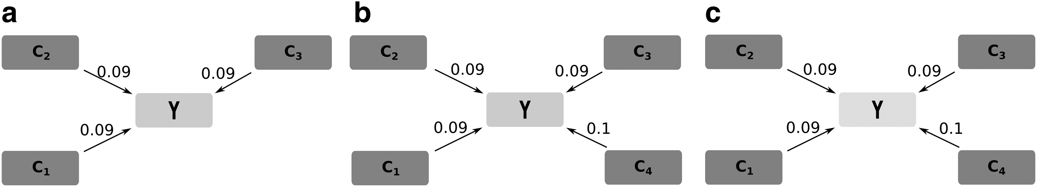
Three examples of different numbers of subsets for the target gene Y: (a) the best predictor subset \documentclass{aastex}\usepackage{amsbsy}\usepackage{amsfonts}\usepackage{amssymb}\usepackage{bm}\usepackage{mathrsfs}\usepackage{pifont}\usepackage{stmaryrd}\usepackage{textcomp}\usepackage{portland, xspace}\usepackage{amsmath, amsxtra}\usepackage{upgreek}\pagestyle{empty}\DeclareMathSizes{10}{9}{7}{6}\begin{document} $$\{ {C_1} , {C_2} , {C_3} \} $$ \end{document} ; (b) top two predictor subsets \documentclass{aastex}\usepackage{amsbsy}\usepackage{amsfonts}\usepackage{amssymb}\usepackage{bm}\usepackage{mathrsfs}\usepackage{pifont}\usepackage{stmaryrd}\usepackage{textcomp}\usepackage{portland, xspace}\usepackage{amsmath, amsxtra}\usepackage{upgreek}\pagestyle{empty}\DeclareMathSizes{10}{9}{7}{6}\begin{document} $$\{ \{ {C_1} , {C_2} , {C_3} \} , \{ {C_4} \} \} $$ \end{document} ; (c) top three predictor subsets \documentclass{aastex}\usepackage{amsbsy}\usepackage{amsfonts}\usepackage{amssymb}\usepackage{bm}\usepackage{mathrsfs}\usepackage{pifont}\usepackage{stmaryrd}\usepackage{textcomp}\usepackage{portland, xspace}\usepackage{amsmath, amsxtra}\usepackage{upgreek}\pagestyle{empty}\DeclareMathSizes{10}{9}{7}{6}\begin{document} $$\{ \{ {C_1} , {C_2} , {C_3} \} , \{ {C_4} \} , \{ {C_5} , {C_6} \} \} $$ \end{document} . The edges represent the predictive power of the predictor subsets with regard to the target gene according to a given criterion function. The smaller the value, the greater the predictive power.

Once defined the final predictor subsets for each target, the dependence logics that rule the target expression profile based on its final predictor subset are derived, as shown in Fig. 4b. These dependence logics are retrieved from the conditional probability distributions \documentclass{aastex}\usepackage{amsbsy}\usepackage{amsfonts}\usepackage{amssymb}\usepackage{bm}\usepackage{mathrsfs}\usepackage{pifont}\usepackage{stmaryrd}\usepackage{textcomp}\usepackage{portland, xspace}\usepackage{amsmath, amsxtra}\usepackage{upgreek}\pagestyle{empty}\DeclareMathSizes{10}{9}{7}{6}\begin{document} $$P ( Y \vert { \bf{Z}} )$$ \end{document} (where Y is the target and Z is a candidate predictor subset for Y), in such a way that for all \documentclass{aastex}\usepackage{amsbsy}\usepackage{amsfonts}\usepackage{amssymb}\usepackage{bm}\usepackage{mathrsfs}\usepackage{pifont}\usepackage{stmaryrd}\usepackage{textcomp}\usepackage{portland, xspace}\usepackage{amsmath, amsxtra}\usepackage{upgreek}\pagestyle{empty}\DeclareMathSizes{10}{9}{7}{6}\begin{document} $${ \bf{z}} \in { \bf{Z}}$$ \end{document} , the Y output is defined by \documentclass{aastex}\usepackage{amsbsy}\usepackage{amsfonts}\usepackage{amssymb}\usepackage{bm}\usepackage{mathrsfs}\usepackage{pifont}\usepackage{stmaryrd}\usepackage{textcomp}\usepackage{portland, xspace}\usepackage{amsmath, amsxtra}\usepackage{upgreek}\pagestyle{empty}\DeclareMathSizes{10}{9}{7}{6}\begin{document} $$\{ y \vert P ( Y = y \vert { \bf{Z}} = { \bf{z}} ) = \mathop { \max } \nolimits_{y \in Y} \ P ( Y = y \vert { \bf{Z}} = { \bf{z}} ) \} $$ \end{document} (the logic outputs are those that minimize the Bayesian classification error of Y based on Z values). This results in the final inferred PGN.

2.8. Computational complexity analysis

As the computational complexity of the framework is mainly given by the exhaustive search algorithm in the Feature Selection step (step d), we focus only on the analysis of the complexity of this step. The other steps have a negligible processing time in comparison, since they are processed in seconds even for very big data sets. Hence, the complexity is measured according to the number of times that the criterion function is calculated during the Feature Selection step (so let us assume that one criterion function calculation presents \documentclass{aastex}\usepackage{amsbsy}\usepackage{amsfonts}\usepackage{amssymb}\usepackage{bm}\usepackage{mathrsfs}\usepackage{pifont}\usepackage{stmaryrd}\usepackage{textcomp}\usepackage{portland, xspace}\usepackage{amsmath, amsxtra}\usepackage{upgreek}\pagestyle{empty}\DeclareMathSizes{10}{9}{7}{6}\begin{document} $${ \cal O} ( 1 )$$ \end{document} time, which is true for fixed small predictor subset cardinalities and fixed small number of possible discrete expression values).

Let N be the number of genes in the data set \documentclass{aastex}\usepackage{amsbsy}\usepackage{amsfonts}\usepackage{amssymb}\usepackage{bm}\usepackage{mathrsfs}\usepackage{pifont}\usepackage{stmaryrd}\usepackage{textcomp}\usepackage{portland, xspace}\usepackage{amsmath, amsxtra}\usepackage{upgreek}\pagestyle{empty}\DeclareMathSizes{10}{9}{7}{6}\begin{document} $$( N = \vert { \bf{X}} \vert )$$ \end{document} , p be the fixed number of predictors for a predictor subset, and k be the number of clusters obtained in step b. The complexity of inferring the GN topology using the exhaustive search is given by \documentclass{aastex}\usepackage{amsbsy}\usepackage{amsfonts}\usepackage{amssymb}\usepackage{bm}\usepackage{mathrsfs}\usepackage{pifont}\usepackage{stmaryrd}\usepackage{textcomp}\usepackage{portland, xspace}\usepackage{amsmath, amsxtra}\usepackage{upgreek}\pagestyle{empty}\DeclareMathSizes{10}{9}{7}{6}\begin{document} $${ \cal O} \left( {N \times \left( { \begin{matrix} k \\ p \\ \end{matrix} } \right) } \right) = { \cal O} ( N \times {k^p} )$$ \end{document} . Since k is expected to be much smaller than N (k is in the order of tens while N is in the order of thousands), the gain in computational time is substantial when compared to the pure exhaustive search, which presents complexity \documentclass{aastex}\usepackage{amsbsy}\usepackage{amsfonts}\usepackage{amssymb}\usepackage{bm}\usepackage{mathrsfs}\usepackage{pifont}\usepackage{stmaryrd}\usepackage{textcomp}\usepackage{portland, xspace}\usepackage{amsmath, amsxtra}\usepackage{upgreek}\pagestyle{empty}\DeclareMathSizes{10}{9}{7}{6}\begin{document} $${ \cal O} \left( {N \times \left( { \begin{matrix} N \\ p \\ \end{matrix} } \right) } \right) = { \cal O} ( {N^{p + 1}} )$$ \end{document} . For example, in a data set with N = 1000 and p = 3, the number of criterion function evaluations is ∼1.66 × 10¹¹ for the pure exhaustive search and 1.62 × 10⁸ for GeNICE with k = 100 (three orders of magnitude below).

2.9. Implemented software

The proposed framework was implemented as a Java plugin^* for Cytoscape (Shannon et al., 2003). It allows advanced analysis of gene expression data through an intuitive graphical user interface, including two other frameworks: MultiExperiment Viewer (MeV) (Howe et al., 2011) and Environment for Developing KDD-Applications Supported by Index-Structures (ELKI) (Achtert et al., 2010). Such a plugin is an evolution of the DimReduction feature selection environment (Lopes et al., 2008).

3. Experimental Setup

To evaluate our framework, we performed experiments with two data sets: (1) simulated (in silico) data and (2) real microarray data. In this section, we describe the protocols adopted in these experiments and the assessment made. Fig. 7 gives an overview of the evaluation process.

FIG. 7.

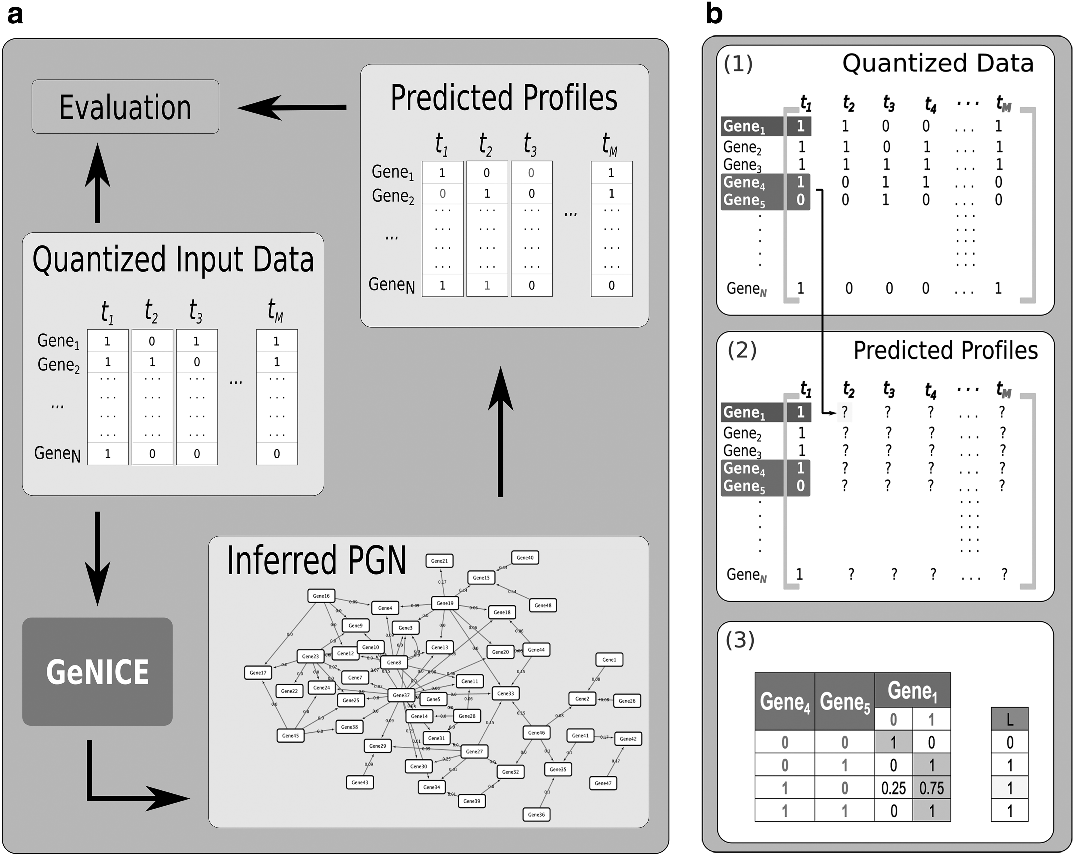
Evaluation of the framework: (a) overview of the evaluation process; (b) some details on how to obtain the predicted profile of a gene Y at time t₂ based on its best subset of predictors Z at time t₁. The same reasoning is applied to all pairs of consecutive time points and for all genes.

3.1. In silico expression data

1. Input data generation: We adopted the SysGenSIM (Pinna et al., 2011) to generate expression data. It is an in silico method that generates gene expression profiles from nonlinear differential equations based on biochemical dynamics of yeasts. This method was applied to generate the DREAM5 Challenges database (Marbach et al., 2012). The following parameters were defined when generating the data sets: three different expression profiles were generated with 40 samples (M = 40) each. The Barabási-Albert scale-free model (Barabási and Albert, 1999) was adopted to generate the network topology, and the average input degree was set to 3. The number of genes was set to \documentclass{aastex}\usepackage{amsbsy}\usepackage{amsfonts}\usepackage{amssymb}\usepackage{bm}\usepackage{mathrsfs}\usepackage{pifont}\usepackage{stmaryrd}\usepackage{textcomp}\usepackage{portland, xspace}\usepackage{amsmath, amsxtra}\usepackage{upgreek}\pagestyle{empty}\DeclareMathSizes{10}{9}{7}{6}\begin{document} $$N \in \{ 100 , 1000 , 5000 \} $$ \end{document} . The cooperativity coefficient was set to a Gamma distribution and the degradation rate was constant. The biological variance of transcription, degradation, and noise was set to a Gaussian distribution, and the other parameters were set to the default values provided by the simulator. These parameters should be defined such that the distribution of estimated heritabilities of the traits is close to those found in real data (Liu et al., 2008).

2. Clustering step: In the clustering step, the Lloyd k-means algorithm (Lloyd, 1982), was adopted to group genes with similar expression profiles. The parameter k, which indicates the number of clusters, was varied considering \documentclass{aastex}\usepackage{amsbsy}\usepackage{amsfonts}\usepackage{amssymb}\usepackage{bm}\usepackage{mathrsfs}\usepackage{pifont}\usepackage{stmaryrd}\usepackage{textcomp}\usepackage{portland, xspace}\usepackage{amsmath, amsxtra}\usepackage{upgreek}\pagestyle{empty}\DeclareMathSizes{10}{9}{7}{6}\begin{document} $$k \in \{ 20 , 30 , 40 , 50 , 100 \} $$ \end{document} , and both Euclidean distance and absolute Pearson correlation were adopted as distance criteria.

3. Feature selection: An exhaustive search for candidate predictor sets of size p = 3 for all N genes placed as target in their turns was applied, adopting the CoD [Eq. (1)] and entropy [Eq. (2)] as criterion functions. It is important to recall that candidate predictors are only the representative genes of the clusters retrieved in the clustering step (one for each of the k clusters).

4. Multivariate analysis: A predictor subset Z was considered, not IMP, with regard to the target Y only if \documentclass{aastex}\usepackage{amsbsy}\usepackage{amsfonts}\usepackage{amssymb}\usepackage{bm}\usepackage{mathrsfs}\usepackage{pifont}\usepackage{stmaryrd}\usepackage{textcomp}\usepackage{portland, xspace}\usepackage{amsmath, amsxtra}\usepackage{upgreek}\pagestyle{empty}\DeclareMathSizes{10}{9}{7}{6}\begin{document} $$IS = 0$$ \end{document} (in this case, the method proceeds to the removal of redundant features).

5. PGN construction: Only the best subset for each target gene was considered to compose the network and to generate the prediction logics.

6. Evaluation: To evaluate the inferred gene expression profile dynamics, first the expression data of a gene at the time \documentclass{aastex}\usepackage{amsbsy}\usepackage{amsfonts}\usepackage{amssymb}\usepackage{bm}\usepackage{mathrsfs}\usepackage{pifont}\usepackage{stmaryrd}\usepackage{textcomp}\usepackage{portland, xspace}\usepackage{amsmath, amsxtra}\usepackage{upgreek}\pagestyle{empty}\DeclareMathSizes{10}{9}{7}{6}\begin{document} $${t_{i + 1}}$$ \end{document} are generated by the application of the prediction logic of its corresponding predictors by taking its expression values from time t_i obtained from the quantized data set as input. This is performed considering all genes and all time points, which leads to the profiles predicted by the inferred PGN. Second, an accuracy value is assigned to each target gene as the percentage of time points (one for each sample in the quantized data set), in which the predictor subset was able to correctly define the next expression value of the target gene. Each inferred binary gene expression profile is compared with the corresponding binary gene expression profile from the quantized data set. Fig. 7a provides an overview of this evaluation process, whereas Fig. 7b shows in more detail how to achieve the predicted profiles from the inferred PGN.

The percentage of correctly predicted time points for a given gene defines its accuracy (it is equivalent to the Hamming distance between two binary profiles divided by the number of time points present in the data set). The average of accuracies obtained for all target genes is taken as the overall accuracy of the inferred data set (values between 0 and 1, where 1 means perfect accuracy and 0.5 is the expected value obtained by random guesses of the binary gene expression profile values) (Qian and Dougherty, 2013).

3.2. P. falciparum microarray expression data

In this experiment, we adopted gene expression data from the transcriptome of the intraerythrocytic developmental cycle (IDC) of the P. falciparum (a malaria agent). This transcriptome was generated by relative measurements of abundance levels of mRNA from samples collected from a strain called HB3, which is well characterized and originated from Honduras (Bozdech et al., 2003). The quality control data set (called QC data set) containing 48 time point samples with N = 5080 genes was used in this experiment. These 48 samples were extracted hourly, corresponding to the 48 hours (time instants) of IDC. The time points corresponding to the 23rd and 29th hours were discarded due to bad quality (so we considered time point 22 as predecessor of time point 24, and time point 28 as predecessor of time point 30), which led to M = 46 time point samples. This expression data set contains oligonucleotides from the glycolytic pathway, ribonucleotide synthesis, deoxyribonucleotide synthesis, DNA replication machinery, TCA cycle, proteasome, plastid genome (apicoplast), merozoite invasion, actin myosin motility, early ring transcripts, mitochondrial genes, and organellar translational group.

We adopted seed genes (target genes) from two functional modules, glycolytic pathway and plastid genome (apicoplast), as done in a study (Barrera et al., 2007) to obtain the minimum number of predictors that interconnect all seeds of the same module. The list of seeds, including their respective annotations, is shown in Table 1. It is expected that just a few predictor genes per seed are enough to connect all seeds of the same module and its corresponding predictors in a single connected component. Besides, it is expected that the glycolysis and apicoplast modules form separate components or a single component with a very small intersection of genes predicting seeds from both modules (these genes would be bridges connecting the two modules). In summary, besides expression signal dynamics assessment, here we conduct topological structure assessment to check whether the final network around the seeds presents high intramodularity and small intermodularity, attending an important property of small-world topological model (Strogatz, 2001).

Table 1.

Glycolysis and Apicoplast Seeds Considered in the Plasmodium falciparum Data Set Experiment

Glycolytic seeds			Apicoplast (plastid genome) seeds
Oligo ID	ORF ID	Manual annotation	Oligo ID	ORF ID	Manual annotation
i13056_1	PFI0755c	6-Phosphofructokinase, putative	pclp	Clp	Plastid genome
i1689_2	PFI1105w	Phosphoglycerate kinase	plsu	lsw	Plastid genome
j2896_1	PF11_0208	Phosphoglycerate mutase, putative	porf129	ORF129	Plastid genome
j53_48	PF10_0155	Enolase	porf91	ORF91	Plastid genome
m11919_1	PF14_0425	Fructose-bisphosphate aldolase	prpl4	rpl14	Plastid genome
m48835_1	PF14_0598	Glyceraldehyde-3-phosphate dehydrogenase	prpl16	rpl16	Plastid genome
n132_136	PF14_0341	Glucose-6-phosphate isomerase	prpl2	rpl2	Plastid genome
n132_40	PF14_0378	Triose-phosphate isomerase	prpl23	rpl23	Plastid genome
opff72413	MAL6P1.189	Hexokinase	prpl36	rpl36	Plastid genome
opff72425	MAL6P1.160	Pyruvate kinase, putative	prpl4	rpl4	Plastid genome
			prpl6	rpl6	Plastid genome
			prps11	rps11	Plastid genome
			prps12	rps12	Plastid genome
			prps17	rps17	Plastid genome
			prps19	rps19	Plastid genome
			prps3	rps3	Plastid genome
			prps5	rps5	Plastid genome
			prps7	rps7	Plastid genome
			prps8	rps8	Plastid genome
			ptrgln	trgln	Plastid genome
			ptrgly	trgly	Plastid genome
			ptrgly2	trgly2	Plastid genome
			ptrphe	trphe	Plastid genome
			ptrpro	trpro	Plastid genome
			ptrthr	trthr	Plastid genome
			ptrtrp	trtrp	Plastid genome
			ptufa	tufa	Plastid genome

For the clustering step, regarding expression profile dynamics assessment, we considered \documentclass{aastex}\usepackage{amsbsy}\usepackage{amsfonts}\usepackage{amssymb}\usepackage{bm}\usepackage{mathrsfs}\usepackage{pifont}\usepackage{stmaryrd}\usepackage{textcomp}\usepackage{portland, xspace}\usepackage{amsmath, amsxtra}\usepackage{upgreek}\pagestyle{empty}\DeclareMathSizes{10}{9}{7}{6}\begin{document} $$k \in \{ 20 , 30 , 40 , 50 \} $$ \end{document} as done in silico experiment. For topological assessment, we considered \documentclass{aastex}\usepackage{amsbsy}\usepackage{amsfonts}\usepackage{amssymb}\usepackage{bm}\usepackage{mathrsfs}\usepackage{pifont}\usepackage{stmaryrd}\usepackage{textcomp}\usepackage{portland, xspace}\usepackage{amsmath, amsxtra}\usepackage{upgreek}\pagestyle{empty}\DeclareMathSizes{10}{9}{7}{6}\begin{document} $$k \in \{ 40 , 50 \} $$ \end{document} only, since the accuracies regarding expression profile dynamics assessment were best for both k = 40 and k = 50 (the accuracies for these two k values were very similar, as shown in Section 4).

For the feature selection step, we applied exhaustive search for predictor subsets of dimension p = 3 for every target. We adopted CoD and entropy as criterion functions [Eqs. (1) and (2)].

For the multivariate analysis, we adopted IS (Z, Y) = 0 [Eq. (3)] as criterion to eliminate redundant features, as done for the in silico data experiment.

Finally, for the network construction, we considered the best subset per target gene when performing the expression profile dynamics analysis. Considering the topological structure analysis involving glycolytic and apicoplast seeds, we retrieved the best predictor subset per seed.

3.3. Hardware and software used in the experiments

For the PGN inference, we used the framework implementation (Cytoscape plugin) briefly described in Section 2.9. Experiments were executed on a computer Intel^® Xeon^® 8 core CPU E7-2870 2.40 GHz with 32 GB RAM, under Linux Ubuntu 64-bit operating system.

4. Results and Discussion

In this section, we present gene expression data prediction.

4.1. In silico data experiment

4.1.1. Comparison between GeNICE and pure exhaustive search inference

Here we compare both accuracies and execution times of GRN inference by pure exhaustive search (without clustering step) and by our proposed framework. The pure exhaustive search was performed only for data sets composed of N = 100 genes, since this method requires much computational effort for N > 100 (see Section 2.8). In contrast, GeNICE was executed for data sets composed of \documentclass{aastex}\usepackage{amsbsy}\usepackage{amsfonts}\usepackage{amssymb}\usepackage{bm}\usepackage{mathrsfs}\usepackage{pifont}\usepackage{stmaryrd}\usepackage{textcomp}\usepackage{portland, xspace}\usepackage{amsmath, amsxtra}\usepackage{upgreek}\pagestyle{empty}\DeclareMathSizes{10}{9}{7}{6}\begin{document} $$N \in \{ 100 , 1000 \} $$ \end{document} genes. We evaluated the performance of GeNICE for \documentclass{aastex}\usepackage{amsbsy}\usepackage{amsfonts}\usepackage{amssymb}\usepackage{bm}\usepackage{mathrsfs}\usepackage{pifont}\usepackage{stmaryrd}\usepackage{textcomp}\usepackage{portland, xspace}\usepackage{amsmath, amsxtra}\usepackage{upgreek}\pagestyle{empty}\DeclareMathSizes{10}{9}{7}{6}\begin{document} $$k \in \{ 20 , 30 , 40 , 50 , 100 \} $$ \end{document} , where k is the number of clusters. In this particular experiment, the results are shown only for Euclidean distance as clustering criterion function, since the results for absolute Pearson correlation were similar.

Fig. 8 shows the average prediction accuracy of the inferred expression profiles taking the quantized generated data set as ground truth for different numbers of clusters, involving the comparison between our framework and the pure exhaustive search with N = 100. The corresponding execution times elapsed to obtain the best predictor subsets for a single target are shown in Table 2. For the pure exhaustive search, the time elapsed for N = 1000 was estimated, since it was not executed until completion.

FIG. 8.

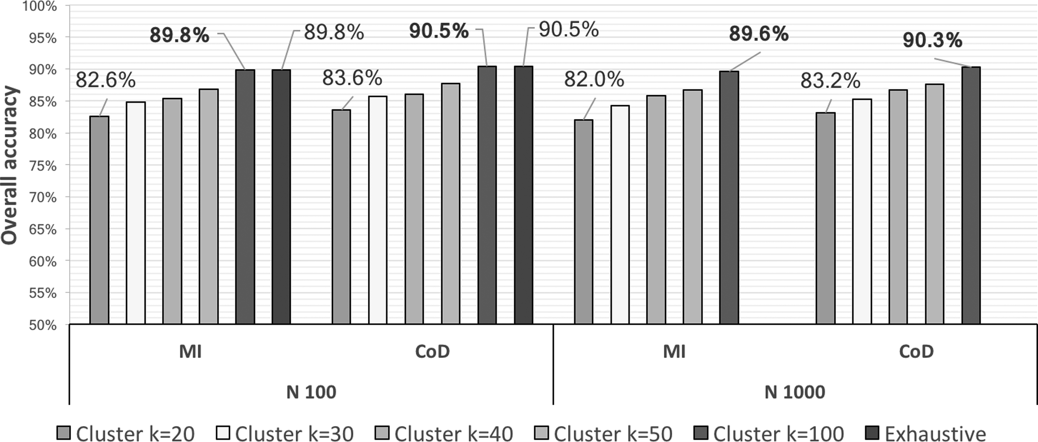
Overall accuracy of GeNICE framework for \documentclass{aastex}\usepackage{amsbsy}\usepackage{amsfonts}\usepackage{amssymb}\usepackage{bm}\usepackage{mathrsfs}\usepackage{pifont}\usepackage{stmaryrd}\usepackage{textcomp}\usepackage{portland, xspace}\usepackage{amsmath, amsxtra}\usepackage{upgreek}\pagestyle{empty}\DeclareMathSizes{10}{9}{7}{6}\begin{document} $$k \in \{ 20 , 30 , 40 , 50 , 100 \} $$ \end{document} and \documentclass{aastex}\usepackage{amsbsy}\usepackage{amsfonts}\usepackage{amssymb}\usepackage{bm}\usepackage{mathrsfs}\usepackage{pifont}\usepackage{stmaryrd}\usepackage{textcomp}\usepackage{portland, xspace}\usepackage{amsmath, amsxtra}\usepackage{upgreek}\pagestyle{empty}\DeclareMathSizes{10}{9}{7}{6}\begin{document} $$N \in \{ 100 , 1000 \} $$ \end{document} , when compared to the pure exhaustive search for N = 100 only (black bars legended by “Exhaustive”).

Table 2.

Processing Time for Entropy and Coefficient of Determination as Criterion Functions Exha: Pure Exhaustive Search

N = 100 genes						N = 1000 genes
	k = 20	k = 30	k = 40	k = 50	Exha.	k = 20	k = 30	k = 40	k = 50	k = 100	Exha.
Entropy time	<1 min	≈1 min	≈3 min	≈6 min	≈29 min	<1 min	≈1 min	≈3 min	≈6 min	≈29 min	^*20 days
CoD time	<1 min	≈1 min	≈2 min	≈5 min	≈28 min	<1 min	≈1 min	≈2 min	≈5 min	≈28 min	^*20 days

It is noteworthy that the accuracy loss was very small when using GeNICE, specially for k = 50 (for N = 100 and k = 1000 are equivalent to pure exhaustive search, since no clustering was involved in this particular case), while the processing time was substantially reduced when compared to the pure exhaustive search. GeNICE spent <30 minutes for all cases, regardless of the number of genes (N), which means that GeNICE is scalable in terms of number of genes.

As predicted by the theoretical complexity analysis (see Section 2.8), in GeNICE, the execution time is only affected by the number of clusters, while the overhead introduced by the clustering and multivariate steps is negligible. In this experiment, the pure exhaustive search, in its turn, is unfeasible to execute for a larger number of genes. According to our estimates, if the pure exhaustive search was fully processed for a single target gene considering N = 1000 genes, it would spend about 28,800 minutes (20 days), which is roughly 1000 times longer than the processing time required by GeNICE framework considering N = 1000 and k = 100. Finally, it is also noteworthy that the accuracies of our framework for N = 1000 and k = 100 were almost identical to the accuracies of the pure exhaustive search for N = 100, even though our framework was applied to a network that was 10 times larger in terms of the number of genes than the one considered for the pure exhaustive search. This observation is remarkable, since real expression data sets usually present dimensionality in the order of thousands, which means that GeNICE can be an useful method in other domains where the exhaustive search is unfeasible.

Regarding the impact of the criterion function in the prediction accuracies achieved, the CoD and mean conditional entropy implied in very close accuracies for all N and k values considered.

4.1.2. Assessment of individual gene expression profile accuracies for increasing k values

In this study, the objective is to assess the prediction accuracy of the dynamics of each individual gene expression profile for increasing k values \documentclass{aastex}\usepackage{amsbsy}\usepackage{amsfonts}\usepackage{amssymb}\usepackage{bm}\usepackage{mathrsfs}\usepackage{pifont}\usepackage{stmaryrd}\usepackage{textcomp}\usepackage{portland, xspace}\usepackage{amsmath, amsxtra}\usepackage{upgreek}\pagestyle{empty}\DeclareMathSizes{10}{9}{7}{6}\begin{document} $$( k \in \{ 20 , 30 , 40 , 50 \} )$$ \end{document} and a network with 5000 genes (N = 5000). Fig. 9 shows box plot distribution of 5000 accuracies (one per target gene) for every triple (k, \documentclass{aastex}\usepackage{amsbsy}\usepackage{amsfonts}\usepackage{amssymb}\usepackage{bm}\usepackage{mathrsfs}\usepackage{pifont}\usepackage{stmaryrd}\usepackage{textcomp}\usepackage{portland, xspace}\usepackage{amsmath, amsxtra}\usepackage{upgreek}\pagestyle{empty}\DeclareMathSizes{10}{9}{7}{6}\begin{document} $${ \cal J}$$ \end{document} , c), where \documentclass{aastex}\usepackage{amsbsy}\usepackage{amsfonts}\usepackage{amssymb}\usepackage{bm}\usepackage{mathrsfs}\usepackage{pifont}\usepackage{stmaryrd}\usepackage{textcomp}\usepackage{portland, xspace}\usepackage{amsmath, amsxtra}\usepackage{upgreek}\pagestyle{empty}\DeclareMathSizes{10}{9}{7}{6}\begin{document} $${ \cal J}$$ \end{document} covers the feature selection criterion functions entropy and CoD, and c covers the clustering criteria: absolute Pearson correlation and Euclidean distance. We observe that there is a general increasing trend of accuracies for increasing k values, as expected. On the contrary, the selection of the clustering criterion does not have a significant impact on the results. Regarding the feature selection criterion choice, the CoD consistently achieved better accuracy results than entropy.

FIG. 9.

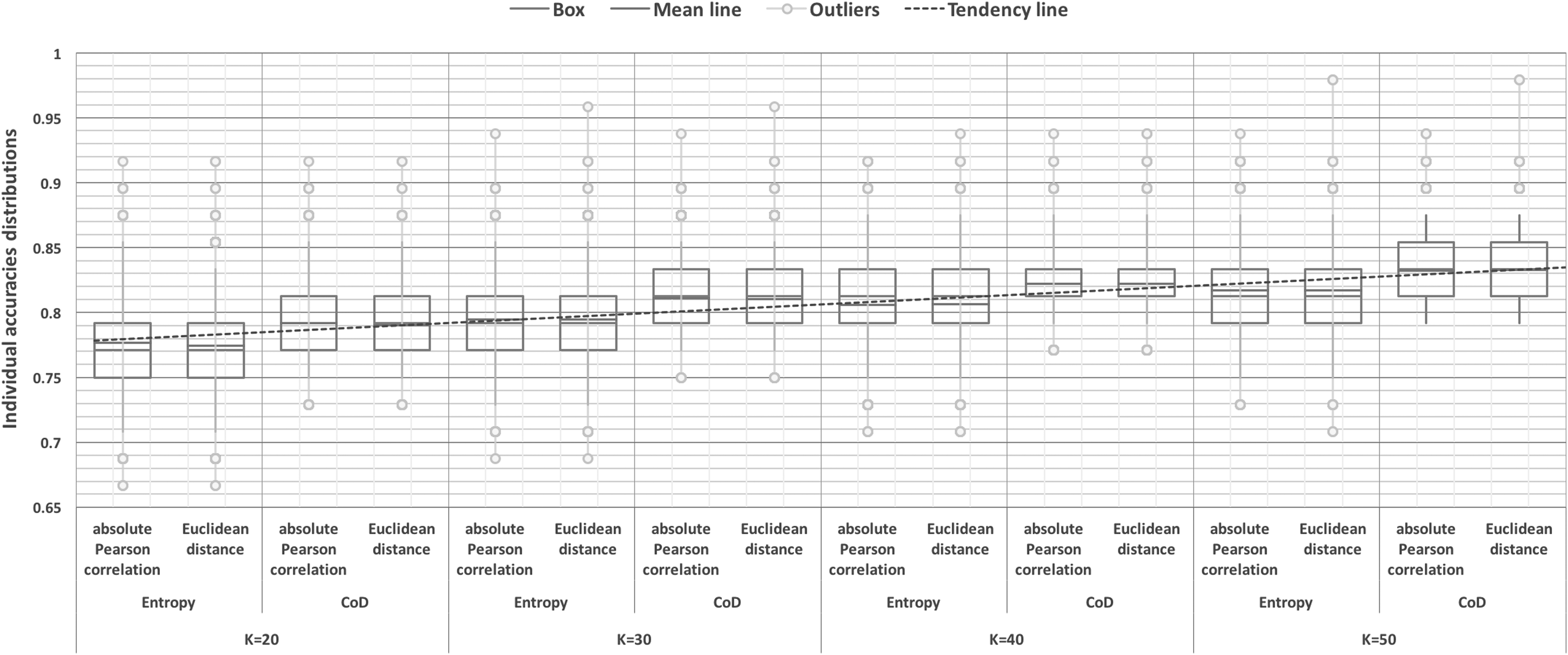
Distribution (box plot) of individual gene expression profile prediction accuracies for every triple (k, \documentclass{aastex}\usepackage{amsbsy}\usepackage{amsfonts}\usepackage{amssymb}\usepackage{bm}\usepackage{mathrsfs}\usepackage{pifont}\usepackage{stmaryrd}\usepackage{textcomp}\usepackage{portland, xspace}\usepackage{amsmath, amsxtra}\usepackage{upgreek}\pagestyle{empty}\DeclareMathSizes{10}{9}{7}{6}\begin{document} $${ \cal J}$$ \end{document} , c) and in silico generated data with 5000 genes (N = 5000). \documentclass{aastex}\usepackage{amsbsy}\usepackage{amsfonts}\usepackage{amssymb}\usepackage{bm}\usepackage{mathrsfs}\usepackage{pifont}\usepackage{stmaryrd}\usepackage{textcomp}\usepackage{portland, xspace}\usepackage{amsmath, amsxtra}\usepackage{upgreek}\pagestyle{empty}\DeclareMathSizes{10}{9}{7}{6}\begin{document} $$k \in \{ 20 , 30 , 40 , 50 \} $$ \end{document} ; \documentclass{aastex}\usepackage{amsbsy}\usepackage{amsfonts}\usepackage{amssymb}\usepackage{bm}\usepackage{mathrsfs}\usepackage{pifont}\usepackage{stmaryrd}\usepackage{textcomp}\usepackage{portland, xspace}\usepackage{amsmath, amsxtra}\usepackage{upgreek}\pagestyle{empty}\DeclareMathSizes{10}{9}{7}{6}\begin{document} $${ \cal J} \in$$ \end{document} {entropy, CoD}; \documentclass{aastex}\usepackage{amsbsy}\usepackage{amsfonts}\usepackage{amssymb}\usepackage{bm}\usepackage{mathrsfs}\usepackage{pifont}\usepackage{stmaryrd}\usepackage{textcomp}\usepackage{portland, xspace}\usepackage{amsmath, amsxtra}\usepackage{upgreek}\pagestyle{empty}\DeclareMathSizes{10}{9}{7}{6}\begin{document} $$c \in$$ \end{document} {absolute Pearson correlation, Euclidean distance}. The dashed black line is the tendency line that best adjusts to the distributions. CoD, coefficient of determination.

4.2. P. falciparum microarray expression data

4.2.1. Assessment of individual gene expression profile accuracies for increasing k values

As done for in silico data, here the objective is to assess the prediction accuracy of the dynamics of each individual gene expression profile for increasing k values \documentclass{aastex}\usepackage{amsbsy}\usepackage{amsfonts}\usepackage{amssymb}\usepackage{bm}\usepackage{mathrsfs}\usepackage{pifont}\usepackage{stmaryrd}\usepackage{textcomp}\usepackage{portland, xspace}\usepackage{amsmath, amsxtra}\usepackage{upgreek}\pagestyle{empty}\DeclareMathSizes{10}{9}{7}{6}\begin{document} $$( k \in \{ 20 , 30 , 40 , 50 \} )$$ \end{document} . Fig. 10 shows box plot distribution of 5080 accuracies (one per target gene) for every triple (k, \documentclass{aastex}\usepackage{amsbsy}\usepackage{amsfonts}\usepackage{amssymb}\usepackage{bm}\usepackage{mathrsfs}\usepackage{pifont}\usepackage{stmaryrd}\usepackage{textcomp}\usepackage{portland, xspace}\usepackage{amsmath, amsxtra}\usepackage{upgreek}\pagestyle{empty}\DeclareMathSizes{10}{9}{7}{6}\begin{document} $${ \cal J}$$ \end{document} , c), where \documentclass{aastex}\usepackage{amsbsy}\usepackage{amsfonts}\usepackage{amssymb}\usepackage{bm}\usepackage{mathrsfs}\usepackage{pifont}\usepackage{stmaryrd}\usepackage{textcomp}\usepackage{portland, xspace}\usepackage{amsmath, amsxtra}\usepackage{upgreek}\pagestyle{empty}\DeclareMathSizes{10}{9}{7}{6}\begin{document} $${ \cal J}$$ \end{document} covers the feature selection criterion functions, entropy and CoD, and c covers the clustering criteria: absolute Pearson correlation and Euclidean distance. We observe that the accuracies reached for all k values are much better than the accuracies for the equivalent in silico experiment (see both Figs. 9 and 10 for comparison). For k = 20 (worst case scenario), the average accuracy was about 95% against 78% for the in silico experiment. For all \documentclass{aastex}\usepackage{amsbsy}\usepackage{amsfonts}\usepackage{amssymb}\usepackage{bm}\usepackage{mathrsfs}\usepackage{pifont}\usepackage{stmaryrd}\usepackage{textcomp}\usepackage{portland, xspace}\usepackage{amsmath, amsxtra}\usepackage{upgreek}\pagestyle{empty}\DeclareMathSizes{10}{9}{7}{6}\begin{document} $$k \ge 30$$ \end{document} , the average accuracies were about 97% against 83% for the best case scenario regarding in silico experiment (k = 50). Anyway, the performances for Plasmodium falciparum were remarkable, since at least 25% of gene expression profiles were perfectly predicted for \documentclass{aastex}\usepackage{amsbsy}\usepackage{amsfonts}\usepackage{amssymb}\usepackage{bm}\usepackage{mathrsfs}\usepackage{pifont}\usepackage{stmaryrd}\usepackage{textcomp}\usepackage{portland, xspace}\usepackage{amsmath, amsxtra}\usepackage{upgreek}\pagestyle{empty}\DeclareMathSizes{10}{9}{7}{6}\begin{document} $$k \ge 30$$ \end{document} (all Q3 bars reached 100% of prediction accuracy). Regarding the choice of criterion function and clustering criterion, the impact in the overall accuracies was negligible in general.

FIG. 10.

Distribution (box plot) of individual gene expression profile prediction accuracies for every triple (k, \documentclass{aastex}\usepackage{amsbsy}\usepackage{amsfonts}\usepackage{amssymb}\usepackage{bm}\usepackage{mathrsfs}\usepackage{pifont}\usepackage{stmaryrd}\usepackage{textcomp}\usepackage{portland, xspace}\usepackage{amsmath, amsxtra}\usepackage{upgreek}\pagestyle{empty}\DeclareMathSizes{10}{9}{7}{6}\begin{document} $${ \cal J}$$ \end{document} , c) and Plasmodium falciparum data set containing 5080 genes (N = 5080). \documentclass{aastex}\usepackage{amsbsy}\usepackage{amsfonts}\usepackage{amssymb}\usepackage{bm}\usepackage{mathrsfs}\usepackage{pifont}\usepackage{stmaryrd}\usepackage{textcomp}\usepackage{portland, xspace}\usepackage{amsmath, amsxtra}\usepackage{upgreek}\pagestyle{empty}\DeclareMathSizes{10}{9}{7}{6}\begin{document} $$k \in \{ 20 , 30 , 40 , 50 \} $$ \end{document} ; \documentclass{aastex}\usepackage{amsbsy}\usepackage{amsfonts}\usepackage{amssymb}\usepackage{bm}\usepackage{mathrsfs}\usepackage{pifont}\usepackage{stmaryrd}\usepackage{textcomp}\usepackage{portland, xspace}\usepackage{amsmath, amsxtra}\usepackage{upgreek}\pagestyle{empty}\DeclareMathSizes{10}{9}{7}{6}\begin{document} $${ \cal J} \in$$ \end{document} {entropy, CoD}; \documentclass{aastex}\usepackage{amsbsy}\usepackage{amsfonts}\usepackage{amssymb}\usepackage{bm}\usepackage{mathrsfs}\usepackage{pifont}\usepackage{stmaryrd}\usepackage{textcomp}\usepackage{portland, xspace}\usepackage{amsmath, amsxtra}\usepackage{upgreek}\pagestyle{empty}\DeclareMathSizes{10}{9}{7}{6}\begin{document} $$c \in$$ \end{document} {absolute Pearson correlation, Euclidean distance}.

4.2.2. Topological assessment involving glycolytic and apicoplast seeds

In this study, the objective is to assess if the network construction considering 10 glycolytic and 27 apicoplast seeds produces large intramodular connection and small intermodular connection, one of the main small-world properties (Strogatz, 2001). Table 3 shows the characteristics of networks retrieved for \documentclass{aastex}\usepackage{amsbsy}\usepackage{amsfonts}\usepackage{amssymb}\usepackage{bm}\usepackage{mathrsfs}\usepackage{pifont}\usepackage{stmaryrd}\usepackage{textcomp}\usepackage{portland, xspace}\usepackage{amsmath, amsxtra}\usepackage{upgreek}\pagestyle{empty}\DeclareMathSizes{10}{9}{7}{6}\begin{document} $$k \in \{ 40 , 50 \} $$ \end{document} , \documentclass{aastex}\usepackage{amsbsy}\usepackage{amsfonts}\usepackage{amssymb}\usepackage{bm}\usepackage{mathrsfs}\usepackage{pifont}\usepackage{stmaryrd}\usepackage{textcomp}\usepackage{portland, xspace}\usepackage{amsmath, amsxtra}\usepackage{upgreek}\pagestyle{empty}\DeclareMathSizes{10}{9}{7}{6}\begin{document} $${ \cal J} \in$$ \end{document} {CoD, entropy}, and \documentclass{aastex}\usepackage{amsbsy}\usepackage{amsfonts}\usepackage{amssymb}\usepackage{bm}\usepackage{mathrsfs}\usepackage{pifont}\usepackage{stmaryrd}\usepackage{textcomp}\usepackage{portland, xspace}\usepackage{amsmath, amsxtra}\usepackage{upgreek}\pagestyle{empty}\DeclareMathSizes{10}{9}{7}{6}\begin{document} $$c \in$$ \end{document} {absolute Pearson correlation, Euclidean distance}, including number of nodes, number of edges, and number of intersections, that is, number of predictors that predict seeds from different biological modules (glycolytic and apicoplast seeds). The network with the smaller number of intersections was for k = 50, absolute Pearson correlation, and CoD: only three. Its corresponding network is displayed in Fig. 11. It is noteworthy that each module presents strong connectivity among the elements: the glycolysis module presents 14 predictors that are not seeds, while the apicoplast presents 17 predictors that are not seeds. In addition, some apicoplast seeds predict each other (interactions between dark gray nodes).

FIG. 11.

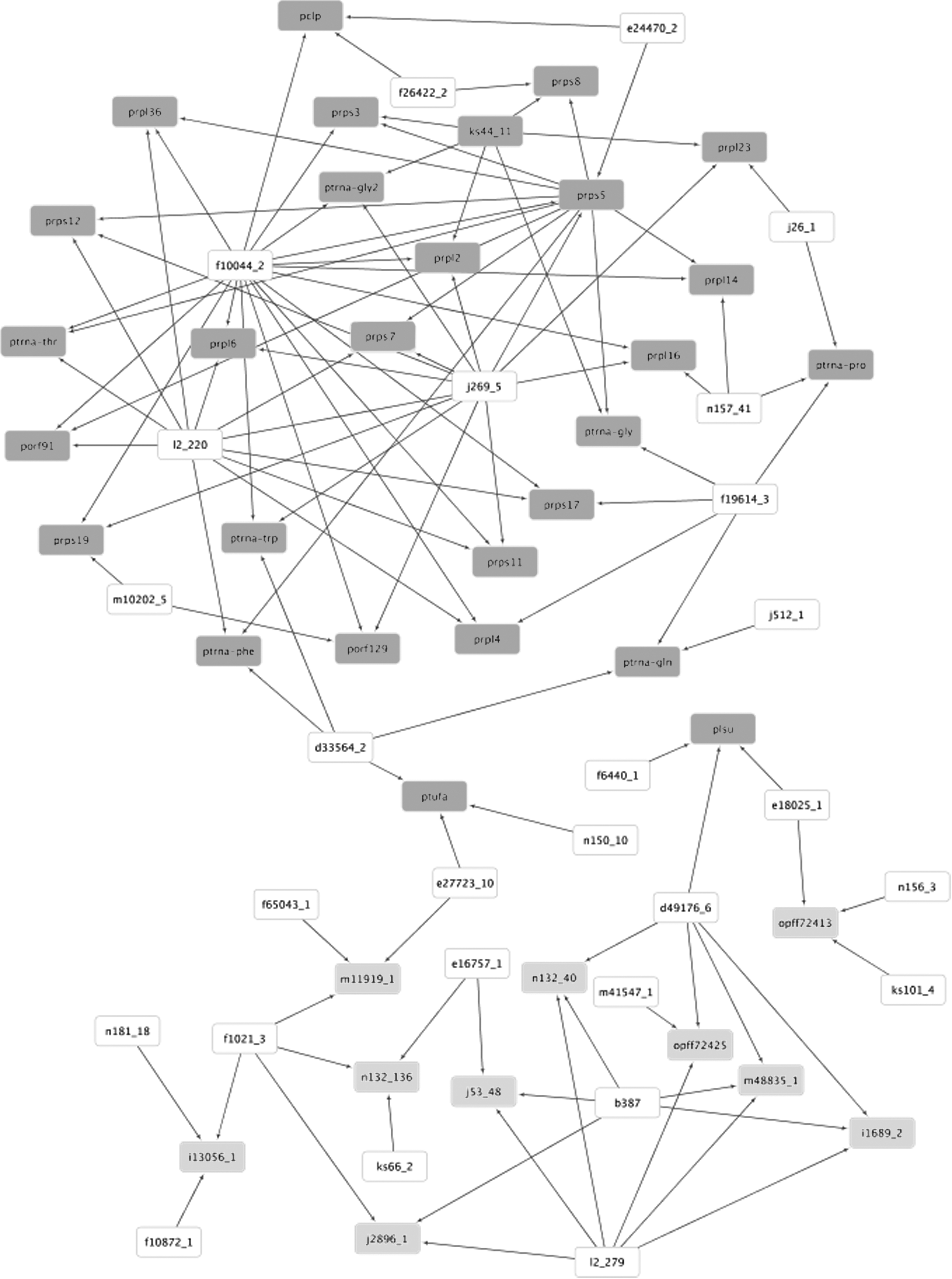
PGN inferred for the glycolytic (light gray nodes) and apicoplast (dark gray nodes) seeds for k = 50, absolute Pearson correlation and CoD. White nodes indicate predictor genes that are not seeds. Network visualization generated in Cytoscape (Shannon et al., 2003).

Table 3.

Numbers of Nodes and Edges for the Networks with the Best Predictor Subset for Each of 10 Glycolytic and 27 Apicoplast Seeds, and the Corresponding Intersections (Number of Predictors That Predict Seeds from Both Modules)

		CoD				Entropy
		k = 40
		Absolute Pearson		Euclidean		Absolute Pearson		Euclidean
	Seeds	Nodes	Edges	Nodes	Edges	Nodes	Edges	Nodes	Edges
Glycolytic	10	24	30	22	30	25	30	25	30
Apicoplast	27	46	81	43	81	49	81	49	81
Intersection		6		5		5		9

		CoD				Entropy
		k = 50
		Absolute Pearson		Euclidean		Absolute Pearson		Euclidean
	Seeds	Nodes	Edges	Nodes	Edges	Nodes	Edges	Nodes	Edges
Glycolytic	10	24	30	26	30	25	30	26	30
Apicoplast	27	44	81	44	81	47	81	46	81
Intersection		3		7		6		6

Another important observation is that there are module hubs (predictors that connect very large number of nodes in comparison to the average), such as the gene f10044_2 (output hub in apicoplast module) and 12_279 in the glycolysis module. These three combined facts (small number of predictors connected to seeds from both modules, large number of predictors inside each module, and some hub modules) suggest that this network presents both small-world and scale-free properties, corroborating other biological network studies (Strogatz, 2001, Barabási and Oltvai, 2004).

In addition, only three or less predictors per seed were enough to connect each module. In comparison, Barrera et al. (2007) (original PGN inference approach, which did not include clustering and multivariate analysis steps) needed 10 best individual predictors or 5 best predictor pairs (10 in total) per seed to connect the glycolytic seeds in a single connected component, while 6 best individual predictors or 3 best pairs (6 in total) per seed were needed to connect the apicoplast seeds. This shows that the PGN approach combined with clustering and multivariate analysis steps is more promising in capturing the existing biological network modularities.

Finally, the gene expression signals for each of the k = 50 clusters generated using Euclidean distance and absolute Pearson correlation for P. falciparum data are shown in Fig. 12. It is noteworthy that most of clusters have strong sinusoidal shape, which corroborates the study by Bozdech et al. (2003) which discovered that the P. falciparum expression data present unusually large number of gene expression profiles with strong sinusoidal shapes (at least 50%). This is an indicative that the decisions taken in the clustering step are leading to biologically meaningful clusters, with beneficial impact to the next steps.

FIG. 12.

Gene expression signals present in each of the k = 50 clusters based on the P. falciparum data set for (a) Euclidean distance. (b) absolute Pearson correlation.

5. Conclusion

In this study, we proposed GeNICE, a new framework for GRN inference, in which the main novelty consists in the application of a clustering method to reduce the complexity of the search for the best predictor subsets per target gene, considering the PGN model. We demonstrated the applicability of GeNICE in experiments using synthetic and P. falciparum gene expression data, for which it was able to preserve the gene expression profile prediction accuracy obtained by the pure exhaustive search while substantially reducing the computational complexity of the search.

Regarding the synthetic data sets involved in the experiments, they were generated by a complex and detailed model (nonlinear differential equations based on biochemical dynamics of yeasts (Pinna et al., 2011)), while the PGN model on which our framework relies is much simpler. Even assuming a simpler model, our framework described the synthetic expression profiles with great accuracy (about 90%) considering data sets with 1000 genes. On the contrary, for much larger networks (5000 genes), the accuracies were smaller. This fact might be related to the choice of parameters to generate the data, especially regarding noise. Besides, PGN assumes strong simplification assumptions to deal with the limitations imposed by the data at hand, which might not be suitable for complex models. However, further studies need to be conducted to confirm these hypotheses.

When considering the gene expression signal prediction accuracies by taking P. falciparum data as input, the results were notably superior to the ones achieved by in silico experiment, reaching about 97% on average for a number of clusters as small as only 30. Moreover, topological structure assessment involving glycolytic and apicoplast seeds displayed large modularity connecting seeds of the same function and a small interconnection between the subnetworks corresponding to the two aforementioned functions. This was achieved with only the best predictor gene subset per seed (at the most three genes). Hub genes were observed in both modules. Such observations are meaningful from the biological point of view, since even a small inferred network was able to display complex network features, usually present in biological networks (small-world and scale-free properties) (Strogatz, 2001; Barabási and Oltvai, 2004).

Besides, as GeNICE consists of a framework, several aspects regarding the different steps involved can be improved. For example, other clustering algorithms can be tested as well as other distance metrics and methods to define the representative genes. Also, the clustering algorithm can be applied after the quantization step, which might lead to clusters with less variability among their respective gene expression profiles. Regarding the multivariate analysis for removal of redundant features, Chen and Braga-Neto (2015) developed a method for automatic determination of the IMP score threshold. The application of this method in this step might lead to better topological structures.

Even though completely understanding and modeling the properties and structures of real biological systems are still an open problem, GeNICE showed promise in assisting professionals of biomedicine and related areas in decision-making regarding the control of the gene regulatory systems dynamics. GeNICE also provides a viable system in environments with limited computing resources, which was not possible considering previous works that applied exhaustive search as a way to guarantee the best predictor subset for each target. In this way, the implementation of this framework as a plugin for Cytoscape (Shannon et al., 2003) is currently under development.

Finally, GeNICE showed to be scalable, since we were able to increase 50 times the number of genes in the input expression data without increase in the processing time of exhaustive feature selection for a single target gene, which implies that the processing time linearly increases with the number of genes in the whole network.

Footnotes

Acknowledgments

We gratefully acknowledge funding from CAPES, CNPq (grants 304955/2014-0, 311608/2014-0), and São Paulo Research Foundation, FAPESP (grants 2011/50761-2, 2015/01587-0, 2015/16310-4, 2016/21047-3).

Author Disclosure Statement

No competing financial interests exist.

References

Achtert

, Kriegel

H.-P.

, Reichert

, et al. 2010. Visual evaluation of outlier detection models, 396–399. In International Conference on Database Systems for Advanced Applications. Springer-verlag, Berlin Heidelberg.

Akutsu

, Miyano

, and Kuhara

1999. Identification of genetic networks from a small number of gene expression patterns under the boolean network model, 17–28. In Azuaje

, and Dopazo

, eds., Proceedings of the Pacific Symposium on Biocomputing (PSB), volume 4. Hawaii, The Orchid at Mauna Lani.

Albert

, and Othmer

H.G.

2003. The topology of the regulatory interactions predicts the expression pattern of the segment polarity genes in drosophila melanogaster. J. Theor. Biol., 223, 1–18.

Azuaje

, and Dopazo

2005. Data Analysis and Visualization in Genomics and Proteomics. John Wiley & Sons.

Bansal

, Belcastro

, Ambesi-Impiombato

, et al. 2007. How to infer gene networks from expression profiles. Mol. Syst. Biol. 3, 78.

Barabási

A.L.

, and Albert

1999. Emergence of scaling in random networks. Science, 286, 509–512.

Barabási

A.-L.

, and Oltvai

Z. N.

2004. Network biology: Understanding the cell's functional organization. Nat. Rev. Genet., 5, 101–113.

Barrera

, Cesar

R.M.

Jr. , Martins

D. C.

Jr. , et al. 2007. Constructing probabilistic genetic networks of plasmodium falciparum from dynamical expression signals of the intraerythrocytic development cycle, 11–26. In Methods of Microarray Data Analysis V, chapter 2. Springer.

Borelli

F.F.

, de Camargo

R.Y.

, Martins

D.C.

Jr. , et al. 2013. Gene regulatory networks inference using a multi-GPU exhaustive search algorithm. BMC Bioinformatics, 14, S5.

10.

Bozdech

, Llinas

, Pulliam

B.L.

, et al. 2003. The transcriptome of the intraerythrocytic developmental cycle of Plasmodium falciparum. PLoS Biol. 1, E5.

11.

Carastan-Santos

, Camargo

R.Y.

, Martins

D.C.

Jr. , et al. 2017. Finding exact hitting set solutions for systems biology applications using heterogeneous GPU clusters. Future Gener. Comput. Syst., 67, 418–429.

12.

Cheadle

, Vawter

M.P.

, Freed

W.J.

, et al. 2003. Analysis of microarray data using Z score transformation. J. Mol. Diagn., 5, 73–81.

13.

Chen

, and Braga-Neto

U.M.

2015. Statistical detection of intrinsically multivariate predictive genes. IEEE/ACM Trans. Comput. Biol. Bioinform. (TCBB)., 12, 951–963.

14.

Cover

T.M.

, and van Campenhout

J.M.

1977. On the possible orderings in the measurement selection problem. IEEE Trans. Syst. Man Cybern., 7, 657–661.

15.

Davidich

M.I.

, and Bornholdt

2008. Boolean network model predicts cell cycle sequence of fission yeast. PLoS One, 3, 1–8.

16.

De-Jong

2002. Modeling and simulation of genetic regulatory systems: A literature review. J. Comput. Biol., 9, 67–103.

17.

De-Smet

, and Marchal

2010. Advantages and limitations of current network inference methods. Nat. Rev. Microbiol., 8, 717–729.

18.

Dougherty

E.R.

, Kim

, and Chen

2000. Coefficient of determination in nonlinear signal processing. Signal Process. 80, 2219–2235.

19.

Espinosa-Soto

, Padilla-Longoria

, and Alvarez-Buylla

E.R.

2004. A gene regulatory network model for cell-fate determination during Arabidopsis thaliana flower development that is robust and recovers experimental gene expression profiles. Plant Cell, 16, 2923–2939.

20.

Faith

, Hayete

, Thaden

, et al. 2007. Large-scale mapping and validation of Escherichia coli transcriptional regulation from a compendium of expression profiles. PLoS Biol. 5, 259–265.

21.

Faure

, Naldi

, Chaouiya

, et al. 2006. Dynamical analysis of a generic boolean model for the control of the mammalian cell cycle. Bioinformatics, 22, e124–e131.

22.

Friedman

, Linial

, Nachman

, et al. 2000. Using bayesian networks to analyze expression data. J Comput. Biol., 7, 601–620.

23.

Govaert

, and Nadif

2013. Co-clustering: Models, Algorithms and Applications. ISTE, Wiley.

24.

Hecker

, Lambeck

, Toepfere

, et al. 2009. Gene regulatory network inference: Data integration in dynamic models: A review. Biosystems, 96, 86–103.

25.

Hira

Z.M.

, and Gillies

D.F.

2015. A review of feature selection and feature extraction methods applied on microarray data. Adv. Bioinformatics, 2015, 198363.

26.

Howe

E.A.

, Sinha

, Schlauch

, et al. 2011. Rna-seq analysis in MeV. Bioinformatics, 27, 3209–3210.

27.

, and Yoo

2004. Cluster ensemble and its applications in gene expression analysis, 297–302. In Proceedings of the Second Conference on Asia-Pacific Bioinformatics, volume 29. Australian Computer Society, Inc.

28.

Ideker

, Thorsson

, and Karp

R.M.

2000. Discovery of regulatory interactions through perturbation: Inference and experimental design, 302–313. In Proceedings of the Pacific Symposium on Biocomputing (PSB), volume 5.

29.

Ivanov

, and Dougherty

E.R.

2006. Modeling genetic regulatory networks: Continuous or discrete?. J. Biol. Syst., 14, 219–229.

30.

Kauffman

S.A.

1969. Metabolic stability and epigenesis in randomly constructed genetic nets. J. Theor. Biol., 22, 437–467.

31.

Lahdesmaki

, and Shmulevich

2003. On learning gene regulatory networks under the boolean network model. Mach. Learn., 52, 147–167.

32.

, Long

, Lu

, et al. 2004. The yeast cell-cycle network is robustly designed. Proc. Natl. Acad. Sci. U. S. A., 101, 4781–4786.

33.

Liang

, Fuhrmane

, and Somogyi

1998. Reveal, a general reverse engineering algorithm for inference of genetic network architectures, 18–29. In Proceedings of the Pacific Symposium on Biocomputing (PSB), volume 3.

34.

Liao

T.W.

2005. Clustering of time series data: A survey. Pattern Recogn. 38, 1857–1874.

35.

Liu

, de La Fuente

, and Hoeschele

2008. Gene network inference via structural equation modeling in genetical genomics experiments. Genetics, 178, 1763–1776.

36.

Lloyd

S.P.

1982. Least squares quantization in pcm. IEEE Trans. Inf. Theory., 28, 129–137.

37.

Lopes

F.M.

, Martins

D.C.

Jr. , Barrera

, et al. 2014. A feature selection technique for inference of graphs from their known topological properties: Revealing scale-free gene regulatory networks. Inf. Sci., 272, 1–15.

38.

Lopes

F.M.

, Martins

D.C.

Jr. , and Cesar

R.M.

Jr.

2008. Dimreduction-interactive graphic environment for dimensionality reduction. arXiv preprint arXiv:0805.3964.

39.

Marbach

, Costello

J.C.

, Küffner

, et al. 2012. Wisdom of crowds for robust gene network inference. Nat. Methods, 9, 796–804.

40.

Margolin

A.A.

, Nemenman

, Basso

, et al. 2006. ARACNE: An algorithm for the reconstruction of gene regulatory networks in a mammalian cellular context. BMC Bioinformatics, 7, S7.

41.

Markowetz

, and Spang

2007. Inferring cellular networks—A review. BMC Bioinformatics, 8, S5.

42.

Martins Jr

D.C.

, Braga-Neto

U.M.

, Hashimoto

R.F.

, et al. 2008. Intrinsically multivariate predictive genes. IEEE J. Sel. Topics Signal Process., 2, 424–439.

43.

Martins

D.C.

Jr. , Oliveira

E.A.

, Braga-Neto

U.M.

, et al. 2013. Signal propagation in bayesian networks and its relationship with intrinsically multivariate predictive variables. Inf. Sci., 225, 18–34.

44.

Meyer

, Kontos

, Lafitte

, et al. 2007. Information theoretic inference of large transcriptional regulatory networks. EURASIP J. Bioinform Syst. Biol., 2007, 1–9.

45.

Nam

, Seo

, and Kim

2006. An efficient top-down search algorithm for learning boolean networks of gene expression. Mach. Learn., 65, 229–245.

46.

Pindah

, Nordin

, Seman

, et al. 2015. Review of dimensionality reduction techniques using clustering algorithm in reconstruction of gene regulatory networks, 172–176. In International Conference on Computer, Communications, and Control Technology (I4CT). IEEE.

47.

Pinna

, Soranzo

, Hoeschele

, et al. 2011. Simulating systems genetics data with SysGenSIM. Bioinformatics, 27, 2459–2462.

48.

Pudil

, Novovicová

, and Kittler

1994. Floating search methods in feature selection. Pattern Recogn. Lett., 15, 1119–1125.

49.

Qian

, and Dougherty

E.R.

2013. Validation of gene regulatory network inference based on controllability. Front. Genet., 4, 272.

50.

Sánchez

, and Thieffry

2001. A logical analysis of the drosophila gap-gene system. J Theor. Biol., 211, 115–141.

51.

Shalon

, Smith

S.J.

, and Brown

P.O.

1996. A DNA microarray system for analyzing complex DNA samples using two-color fluorescent probe hybridization. Genome Res. 639–645.

52.

Shannon

C.E.

2001. A mathematical theory of communication. ACM SIGMOBILE Mobile Comput. Commun. Rev., 5, 3–55.

53.

Shannon

, Markiel

, Ozier

, et al. 2003. Cytoscape: A software environment for integrated models of biomolecular interaction networks. Genome Res. 13, 2498–2504.

54.

Shmulevich

, and Dougherty

E.R.

2014. Genomic Signal Processing. Princeton University Press.

55.

Shmulevich

, Dougherty

E.R.

, Kim

, et al. 2002. Probabilistic Boolean networks: A rule-based uncertainty model for gene regulatory networks. Bioinformatics, 18, 261–274.

56.

Strogatz

S.H.

2001. Exploring complex networks. Nature, 410, 268–276.

57.

Styczynski

M.P.

, and Stephanopoulos

2005. Overview of computational methods for the inference of gene regulatory networks. Comput. Chem. Eng., 29, 519–534.

58.

Velculescu

V.E.

, Zhang

, Vogelstein

, et al. 1995. Serial analysis of gene expression. Science, 270, 484–487.

59.

Wang

, Gerstein

, and Snyder

2009. RNA-Seq: A revolutionary tool for transcriptomics. Nat. Rev. Genet., 10, 57–63.

60.

Zhang

, Qian

, Ouyang

, et al. 2006. “stochastic model of yeast cell-cycle network.”. Physica D, 219, 35–39.