Diagnosis Prediction from Electronic Health Records Using the Binary Diagnosis History Vector Representation

Abstract

Large amounts of rich, heterogeneous information nowadays routinely collected by healthcare providers across the world possess remarkable potential for the extraction of novel medical data and the assessment of different practices in real-world conditions. Specifically in this work, our goal is to use electronic health records (EHRs) to predict progression patterns of future diagnoses of ailments for a particular patient, given the patient's present diagnostic history. Following the highly promising results of a recently proposed approach that introduced the diagnosis history vector representation of a patient's diagnostic record, we introduce a series of improvements to the model and conduct thorough experiments that demonstrate its scalability, accuracy, and practicability in the clinical context. We show that the model is able to capture well the interaction between a large number of ailments that correspond to the most frequent diagnoses, show how the original learning framework can be adapted to increase its prediction specificity, and describe a principled, probabilistic method for incorporating explicit, human clinical knowledge to overcome semantic limitations of the raw EHR data.

1. Introduction

The trend of increased efforts in health data collection and its ready digitization are widely recognized as a major change in the manner medical data are used. In particular, the collection of electronic health records (EHRs) has recently started attracting major translational research efforts in the domains of data mining, knowledge extraction, and machine learning (Christensen and Ellingsen, 2016; Xu et al., 2016). EHRs have already been extensively used in large scale sociodemographic surveys of death causes (RGI-CGHR Collaborators, 2009), clinical epidemiological (Crawford et al., 2010; Bhatnagar et al., 2015; Paul et al., 2015c) and pharmacoepidemiological studies (Lau et al., 2011; Wettermark et al., 2013; Paul et al., 2015b), as well as in the analysis of pharmacovigilance (Nadkarni, 2010; Coloma et al., 2013; Liu et al., 2013), health-related economic effects (Bessou et al., 2015; Canavan et al., 2015), and public health (Kukafka et al., 2007; Menachemi and Collum, 2011; Birkhead et al., 2015; Paul et al., 2015a).

Considering that this research is still in its early stages, it is undeniably wise to refrain from overly ambitious predictions regarding the type of knowledge that may be discovered in this manner, at the very least it is true that few domains of application of the aforesaid techniques hold as much promise for impact. It is sufficient to observe the potential benefits that an increased understanding of complex interactions of lifestyle diseases in the economically developed world could deliver in terms of personalized medicine or healthcare policy (Fan et al., 2016) on the one hand, and a wiser utilization of resources, aid, and educational material in the economically deprived countries on the other (RGI-CGHR Collaborators, 2009), to appreciate the global and overarching potential.

Public healthcare is an issue of major global significance and concern. On one end of the spectrum, the developing world is still plagued by “diseases of poverty,” which are nearly nonexistent in the most technologically developed countries; on the other end, the health risk profile of industrially leading nations has dramatically changed in recent history with an increased skew toward so-called “diseases of affluence,” as illustrated in Figure 1 [data taken from Murray et al. (2001)].

FIG. 1.

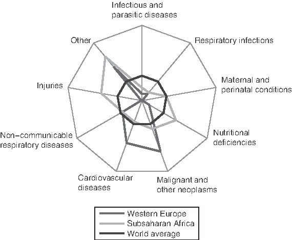
Causes of death for the developed world (western Europe), developing nations (Sub-Saharan Africa), and the world average.

Hence, healthcare management poses challenges in both the sphere of policy making and scientific research. Considering the complexity of problems at hand, it is unsurprising that there is an ever-increasing effort invested in a diverse range of promising avenues. Yet, the available resources are inherently limited. To ensure their best usage, it is crucial both to develop an understanding of the related epidemiology and to be able to communicate this knowledge effectively to those who can benefit from it: governments (Berwick and Hackbarth, 2012), the medical research community (Beykikhoshk et al., 2015a, 2016; Andrei and Arandjelović, 2016), healthcare practitioners (Arandjelović, 2015a; Osuala and Arandjelović, 2017), and patients (Beykikhoshk et al., 2014; Barracliffe et al., 2017).

The associations between diseases and a wide variety of risk factors are underlain by a complex web of interactions. This is particularly the case for the diseases of the developed world. The key premise of this work is to facilitate the understanding of this complexity and the discovery of meaningful patterns within it, it is crucial to make use of the vast amounts of data routinely collected by health services in industrially and technologically developed countries.

Our specific aim is to develop a framework that allows a health practitioner (e.g., a doctor or a clinician) to manipulate the available patient information in an intuitive yet powerful manner. Such a framework would, on one end of the utility spectrum, facilitate a deepening of disease understanding and, on the other, provide the practitioner with a tool that can be used to incentivize the patient at risk to make the required lifestyle changes.

1.1. Data: electronic medical records

This work leverages large amounts of medical data routinely collected and stored in electronic form by health providers in most developed countries. This is a rich data source that contains a variety of information about each patient, including the patient's age and sex, mother tongue, religion, marital status, profession, etc. In the context of this work, of main interest is the information collected each time a patient is admitted to the hospital (including out-patient visits to general practitioners or specialists). The format of these data is explained next.

Each time a patient is admitted to the hospital, the reason for admission, as determined by the medical practitioner in primary charge during the admission, is recorded in the patient's medical history. This is performed using a standardized coding schema such as that provided by the International Statistical Classification of Diseases and Related Health Problems (ICD-10) (World Health Organization, 2004) and the related Australian Refined Diagnosis-Related Groups.

These have hierarchical structures (Arandjelović, 2016). ICD-10, for example, contains 22 chapters, each chapter encompassing a spectrum of related health issues (usually symptomatically rather than etiologically related). For example, ICD-10 Chapter 4, which includes codes E00-E90, covers “endocrine, nutritional, and metabolic diseases.” At each subsequent depth level of the tree, the grouping is refined and the scope of conditions narrowed down. In this article, we use the classification attained at the depth of two of ICD-10, which achieves a good compromise between specificity and frequency of occurrence. This results in each diagnosis being given a three character code that comprises a leading capital letter (A–Z, first grouping level), followed by a two digit number (further refinement). For example, E66 codes for “obesity” within the broader range of “endocrine, nutritional, and metabolic diseases.”

2. Modeling Comorbidity Progression

The major contribution of this work is a novel disease progression model. The principal challenge is posed by the need for a model that is sufficiently flexible to be able to capture complex patterns of comorbidity development, while at the same time constrained enough to facilitate learning from a real-world data corpus.

2.1. Bottom-up modeling

The problem of modeling disease progression has already attracted a considerable amount of research attention. Most previous research focuses on specific individual diseases, such as type 2 diabetes mellitus (Topp et al., 2000; De Gaetano et al., 2008) or heart disease (Ye et al., 2012). These methods are inherently “low-level” based, in the sense that they explicitly model known physiological changes that affect disease progression. For example, the modeling of the progression of type 2 diabetes may include low-level models of \documentclass{aastex}\usepackage{amsbsy}\usepackage{amsfonts}\usepackage{amssymb}\usepackage{bm}\usepackage{mathrsfs}\usepackage{pifont}\usepackage{stmaryrd}\usepackage{textcomp}\usepackage{portland, xspace}\usepackage{amsmath, amsxtra}\usepackage{upgreek}\pagestyle{empty}\DeclareMathSizes{10}{9}{7}{6}\begin{document} $$\beta$$ \end{document} cell mass changes and insulin and glucose dynamics (Topp et al., 2000), with the free parameters (e.g., \documentclass{aastex}\usepackage{amsbsy}\usepackage{amsfonts}\usepackage{amssymb}\usepackage{bm}\usepackage{mathrsfs}\usepackage{pifont}\usepackage{stmaryrd}\usepackage{textcomp}\usepackage{portland, xspace}\usepackage{amsmath, amsxtra}\usepackage{upgreek}\pagestyle{empty}\DeclareMathSizes{10}{9}{7}{6}\begin{document} $$\beta$$ \end{document} cell replication rate) of the models adopted from previous empirical studies. Higher level disease progression then emerges from the interaction of low-level models.

The low-level approach to disease modeling has several limitations. First, by their very nature, these models are limited to specific diseases only and cannot be readily adapted to deal with conditions with entirely different etiologies. Second, the modeling is practically constrained usually to a single condition, two at the most, as the complexity of modeled system increases dramatically with the inclusion of a greater number of conditions. This observation is of major significance as most diseases of the developed world are most often accompanied and affected by multiple comorbidities. Lastly, the range of diseases that can be modeled in this manner is limited to diseases that are sufficiently well understood and studied to allow for the free model parameters to be set reliably; even for type 2 diabetes, which has been studied extensively, at present some parameters must be set in an ad hoc manner and others using in vitro rather than in vivo data (Topp et al., 2000).

2.2. Direct high-level modeling

Given the significance of the disadvantages of low-level-based disease progression models, in this article an alternative approach is pursued, that of seeking to describe disease progression as well as the interplay of different comorbidities directly on the “high-level” as observed by a medical practitioner. Previous research in this area is far scarcer than that on low-level modeling; a possible reason for this is probably to be found in the until recently limited availability of large-scale medical records data. The central idea of the existing corpus of work is to regard disease progression as a discrete sequence of events, with the progression governed by what is assumed to be a first-order Markov process (Jackson et al., 2003; Sukkar et al., 2012).

A high-level view of disease progression is seen as being reflected by a patient's diagnostic history \documentclass{aastex}\usepackage{amsbsy}\usepackage{amsfonts}\usepackage{amssymb}\usepackage{bm}\usepackage{mathrsfs}\usepackage{pifont}\usepackage{stmaryrd}\usepackage{textcomp}\usepackage{portland, xspace}\usepackage{amsmath, amsxtra}\usepackage{upgreek}\pagestyle{empty}\DeclareMathSizes{10}{9}{7}{6}\begin{document} $$H = {d_1} \to {d_2} \to \cdots \to {d_n}$$ \end{document} , where d_i is a discrete variable whose value is a code corresponding to the i-th of n diagnoses on the patient's record. The parameters of the underlying first-order Markov model are then learnt by estimating transition probabilities \documentclass{aastex}\usepackage{amsbsy}\usepackage{amsfonts}\usepackage{amssymb}\usepackage{bm}\usepackage{mathrsfs}\usepackage{pifont}\usepackage{stmaryrd}\usepackage{textcomp}\usepackage{portland, xspace}\usepackage{amsmath, amsxtra}\usepackage{upgreek}\pagestyle{empty}\DeclareMathSizes{10}{9}{7}{6}\begin{document} $$p ( d ^{\prime} \to d ^{\prime \prime} )$$ \end{document} for all transitions encountered during training (the remaining transition probabilities are usually set to some low value rather than 0, using a pseudocount-based estimate) (Bartolomeo et al., 2008; Folino and Pizzuti, 2011; Wang et al., 2014). The model can be applied to predict the diagnosis \documentclass{aastex}\usepackage{amsbsy}\usepackage{amsfonts}\usepackage{amssymb}\usepackage{bm}\usepackage{mathrsfs}\usepackage{pifont}\usepackage{stmaryrd}\usepackage{textcomp}\usepackage{portland, xspace}\usepackage{amsmath, amsxtra}\usepackage{upgreek}\pagestyle{empty}\DeclareMathSizes{10}{9}{7}{6}\begin{document} $${d_{n + 1}}$$ \end{document} expected to follow from the current history by model likelihood maximization: \documentclass{aastex}\usepackage{amsbsy}\usepackage{amsfonts}\usepackage{amssymb}\usepackage{bm}\usepackage{mathrsfs}\usepackage{pifont}\usepackage{stmaryrd}\usepackage{textcomp}\usepackage{portland, xspace}\usepackage{amsmath, amsxtra}\usepackage{upgreek}\pagestyle{empty}\DeclareMathSizes{10}{9}{7}{6}\begin{document} \begin{align*} {d_{n + 1}} = \arg \mathop { \max } \limits_d \ p ( {d_n} \to d ). \tag{1} \end{align*} \end{document}

Alternatively, it may be used to estimate the probability of a particular diagnosis \documentclass{aastex}\usepackage{amsbsy}\usepackage{amsfonts}\usepackage{amssymb}\usepackage{bm}\usepackage{mathrsfs}\usepackage{pifont}\usepackage{stmaryrd}\usepackage{textcomp}\usepackage{portland, xspace}\usepackage{amsmath, amsxtra}\usepackage{upgreek}\pagestyle{empty}\DeclareMathSizes{10}{9}{7}{6}\begin{document} $${d^*}$$ \end{document} at some point in the future: \documentclass{aastex}\usepackage{amsbsy}\usepackage{amsfonts}\usepackage{amssymb}\usepackage{bm}\usepackage{mathrsfs}\usepackage{pifont}\usepackage{stmaryrd}\usepackage{textcomp}\usepackage{portland, xspace}\usepackage{amsmath, amsxtra}\usepackage{upgreek}\pagestyle{empty}\DeclareMathSizes{10}{9}{7}{6}\begin{document} \begin{align*} {p_f} ( {d^*} ) = \mathop \sum \limits_d [ p ( d \to {d^*} ) {p_f} ( d ) ] , \tag{2} \end{align*} \end{document}

or to sample the space of possible histories: \documentclass{aastex}\usepackage{amsbsy}\usepackage{amsfonts}\usepackage{amssymb}\usepackage{bm}\usepackage{mathrsfs}\usepackage{pifont}\usepackage{stmaryrd}\usepackage{textcomp}\usepackage{portland, xspace}\usepackage{amsmath, amsxtra}\usepackage{upgreek}\pagestyle{empty}\DeclareMathSizes{10}{9}{7}{6}\begin{document} \begin{align*} H ^{\prime} = {d_1} \to {d_2} \to \cdots \to {d_n} \to {d_{n + 1}} \to {d_{n + 2}} \ldots .. \tag{3} \end{align*} \end{document}

The primary purpose of the Markovian assumption is to constrain the mechanism underlying a specific process and thus formulate it in a manner that leads to a tractable learning problem. Although it is seldom strictly true, that it is often a reasonable approximation to make is witnessed by its successful application across a diverse range of disciplines; examples of modeled phenomena include meteorological events (Gabriel and Neumann, 1962), software usage patterns (Whittaker and Thomason, 1994), breast cancer screening (Duffy and Yau, 1995), human motion and behavior (Lee et al., 2005; Arandjelović, 2011), and many others. Nonetheless, the key premise motivating the model in this article is that the Markovian assumption is in fact not appropriate for the high-level modeling of disease progression (note that this does not reject its possible applicability in disease progression modeling on different levels of abstraction). Indeed, we demonstrate this empirically. The aforementioned premise is readily substantiated using a theoretical argument as well. Consider a patient who is admitted for what is diagnosed as a serious chronic illness. If the same patient is subsequently admitted for an unrelated ailment, possibly a trivial one, the knowledge of the serious underlying problem is lost and the power to predict the next related diagnosis is lost. The model proposed in the following section solves this problem, while simultaneously retaining the tractability of Markov process-based approaches.

2.3. Proposed approach

In this article, our aim is to predict the probability of a specific diagnosis a following the patient history H: \documentclass{aastex}\usepackage{amsbsy}\usepackage{amsfonts}\usepackage{amssymb}\usepackage{bm}\usepackage{mathrsfs}\usepackage{pifont}\usepackage{stmaryrd}\usepackage{textcomp}\usepackage{portland, xspace}\usepackage{amsmath, amsxtra}\usepackage{upgreek}\pagestyle{empty}\DeclareMathSizes{10}{9}{7}{6}\begin{document} \begin{align*} p ( H \to a \vert H ). \tag{4} \end{align*} \end{document}

The difficulty of formulating this as a tractable learning problem lies in the fact that the space of possible histories is infinite as H can be of an arbitrary length. Even if the length \documentclass{aastex}\usepackage{amsbsy}\usepackage{amsfonts}\usepackage{amssymb}\usepackage{bm}\usepackage{mathrsfs}\usepackage{pifont}\usepackage{stmaryrd}\usepackage{textcomp}\usepackage{portland, xspace}\usepackage{amsmath, amsxtra}\usepackage{upgreek}\pagestyle{empty}\DeclareMathSizes{10}{9}{7}{6}\begin{document} $$l ( H )$$ \end{document} is limited, the number of possible histories is extremely large: \documentclass{aastex}\usepackage{amsbsy}\usepackage{amsfonts}\usepackage{amssymb}\usepackage{bm}\usepackage{mathrsfs}\usepackage{pifont}\usepackage{stmaryrd}\usepackage{textcomp}\usepackage{portland, xspace}\usepackage{amsmath, amsxtra}\usepackage{upgreek}\pagestyle{empty}\DeclareMathSizes{10}{9}{7}{6}\begin{document} $${ [ l ( H ) ] ^{{n_a}}}$$ \end{document} , where n_a is the number of different diagnosis codes. Therefore, it is necessary to make an approximation that constrains and simplifies the task. We already argued why the Markovian assumption on the level of diagnosis codes is inappropriate. In its stead, we propose a different representation of a patient's state, particularly suitable for the modeling of disease progression (Arandjelović, 2015b). Consider a particular diagnosis history \documentclass{aastex}\usepackage{amsbsy}\usepackage{amsfonts}\usepackage{amssymb}\usepackage{bm}\usepackage{mathrsfs}\usepackage{pifont}\usepackage{stmaryrd}\usepackage{textcomp}\usepackage{portland, xspace}\usepackage{amsmath, amsxtra}\usepackage{upgreek}\pagestyle{empty}\DeclareMathSizes{10}{9}{7}{6}\begin{document} $$H = {d_1} \to \cdots \to {d_n}$$ \end{document} . The proposed method makes use of the well-known observation that when it comes to chronic diseases, the very presence of past complications strongly predicts future complications (Friedman et al., 2008–2009; Mudge et al., 2011; Butler and Kalogeropoulos, 2012; Dharmarajan et al., 2013). Thus, a history H is represented using a history vector \documentclass{aastex}\usepackage{amsbsy}\usepackage{amsfonts}\usepackage{amssymb}\usepackage{bm}\usepackage{mathrsfs}\usepackage{pifont}\usepackage{stmaryrd}\usepackage{textcomp}\usepackage{portland, xspace}\usepackage{amsmath, amsxtra}\usepackage{upgreek}\pagestyle{empty}\DeclareMathSizes{10}{9}{7}{6}\begin{document} $$v = v ( H )$$ \end{document} , which is a fixed length vector with binary values (Beykikhoshk et al., 2015b). Each vector element corresponds to a specific diagnosis code (except for one special element explained shortly) and its value is 1 if and only if the corresponding diagnosis is present in the history: \documentclass{aastex}\usepackage{amsbsy}\usepackage{amsfonts}\usepackage{amssymb}\usepackage{bm}\usepackage{mathrsfs}\usepackage{pifont}\usepackage{stmaryrd}\usepackage{textcomp}\usepackage{portland, xspace}\usepackage{amsmath, amsxtra}\usepackage{upgreek}\pagestyle{empty}\DeclareMathSizes{10}{9}{7}{6}\begin{document} \begin{align*} \forall d \in D. v{ ( H ) _{i ( d ) }} = \left\{ { \begin{matrix} {1:} \hfill & { \exists \ j. H = {H_1} \to {d_j} \to {H_2} \wedge d = {d_j}} \hfill \\ {0:} \hfill & {{ \mathop{ \rm otherwise} \nolimits} } \hfill \\ \end{matrix} } \right. , \end{align*} \end{document}

where D is the set of diagnosis codes, \documentclass{aastex}\usepackage{amsbsy}\usepackage{amsfonts}\usepackage{amssymb}\usepackage{bm}\usepackage{mathrsfs}\usepackage{pifont}\usepackage{stmaryrd}\usepackage{textcomp}\usepackage{portland, xspace}\usepackage{amsmath, amsxtra}\usepackage{upgreek}\pagestyle{empty}\DeclareMathSizes{10}{9}{7}{6}\begin{document} $$i ( d )$$ \end{document} indexes the diagnosis code d in a history vector, and \documentclass{aastex}\usepackage{amsbsy}\usepackage{amsfonts}\usepackage{amssymb}\usepackage{bm}\usepackage{mathrsfs}\usepackage{pifont}\usepackage{stmaryrd}\usepackage{textcomp}\usepackage{portland, xspace}\usepackage{amsmath, amsxtra}\usepackage{upgreek}\pagestyle{empty}\DeclareMathSizes{10}{9}{7}{6}\begin{document} $${H_{1 , 2}}$$ \end{document} may take on degenerate forms of empty histories. By collapsing an arbitrary length history of diagnoses onto a fixed length vector, the space of possible states over which learning is performed is dramatically reduced and the problem immediately made far more tractable. Notice the importance of the observation that it is the presence of past complications that most strongly predicts future ailments, given that under this representation any information on the ordering of diagnoses is discarded. The binary nature of the representation also has the effect of reducing the size of the space over which inference is performed. In this case, this is achieved by discarding information on the number of repeated diagnoses, and in this manner it too predicates the overwhelming predictive power of the presence of history of a particular ailment, rather than the number of the corresponding diagnoses.

The disease progression modeling problem at hand is thus reduced to the task of learning transition probabilities between different patient history vectors: \documentclass{aastex}\usepackage{amsbsy}\usepackage{amsfonts}\usepackage{amssymb}\usepackage{bm}\usepackage{mathrsfs}\usepackage{pifont}\usepackage{stmaryrd}\usepackage{textcomp}\usepackage{portland, xspace}\usepackage{amsmath, amsxtra}\usepackage{upgreek}\pagestyle{empty}\DeclareMathSizes{10}{9}{7}{6}\begin{document} \begin{align*} p ( v ( H ) \to v ( H ^{\prime} ) ). \tag{5} \end{align*} \end{document}

It is important to observe that unlike in the case of Markov process models working on the diagnosis level when the number of possible transition probabilities is close to \documentclass{aastex}\usepackage{amsbsy}\usepackage{amsfonts}\usepackage{amssymb}\usepackage{bm}\usepackage{mathrsfs}\usepackage{pifont}\usepackage{stmaryrd}\usepackage{textcomp}\usepackage{portland, xspace}\usepackage{amsmath, amsxtra}\usepackage{upgreek}\pagestyle{empty}\DeclareMathSizes{10}{9}{7}{6}\begin{document} $$n_a^2$$ \end{document} , here the transition space is far sparser. Specifically, note that it is impossible to observe a transition from a history vector that codes for the existence of a particular past diagnosis to one that does not, that is: \documentclass{aastex}\usepackage{amsbsy}\usepackage{amsfonts}\usepackage{amssymb}\usepackage{bm}\usepackage{mathrsfs}\usepackage{pifont}\usepackage{stmaryrd}\usepackage{textcomp}\usepackage{portland, xspace}\usepackage{amsmath, amsxtra}\usepackage{upgreek}\pagestyle{empty}\DeclareMathSizes{10}{9}{7}{6}\begin{document} \begin{align*} v{ ( H ) _{i ( d ) }} = 1 \wedge v{ ( H ^{\prime} ) _{i ( d ) }} = 0 \rightarrow p ( v ( H ) \to v ( H ^{\prime} ) ) = 0. \tag{6} \end{align*} \end{document}

The converse does not hold however. Moreover, possible transitions can be only those that include either no changes to the history vector (repeated diagnosis) or that encode exactly one additional diagnosis: \documentclass{aastex}\usepackage{amsbsy}\usepackage{amsfonts}\usepackage{amssymb}\usepackage{bm}\usepackage{mathrsfs}\usepackage{pifont}\usepackage{stmaryrd}\usepackage{textcomp}\usepackage{portland, xspace}\usepackage{amsmath, amsxtra}\usepackage{upgreek}\pagestyle{empty}\DeclareMathSizes{10}{9}{7}{6}\begin{document} \begin{align*} & p ( v ( H ) \to v ( H ^{\prime} ) ) \\ & \quad \begin{cases} > 0: & \forall a. v ( H )_{i ( d ) } = 1 \rightarrow v( H ^{\prime} )_{i ( d ) } = 1 \\ & {{ \rm{and}}} \\ & \vert \{ a:v ( H )_{i ( d ) } = 1 \} \vert \le 1 + \vert \{ a:v ( H ^{\prime} )_{i ( d ) } = 1 \} \vert \\ = 0: & {{ \rm{otherwise}}} \end{cases} . \tag{7} \end{align*} \end{document}

This gives the upper bound for the number of nonzero probability transitions of \documentclass{aastex}\usepackage{amsbsy}\usepackage{amsfonts}\usepackage{amssymb}\usepackage{bm}\usepackage{mathrsfs}\usepackage{pifont}\usepackage{stmaryrd}\usepackage{textcomp}\usepackage{portland, xspace}\usepackage{amsmath, amsxtra}\usepackage{upgreek}\pagestyle{empty}\DeclareMathSizes{10}{9}{7}{6}\begin{document} $${n_a} \times {2^{{n_a}}}$$ \end{document} . In practice, the actual number of transitions is far smaller (several orders of magnitude for the data set described in the next section), which allows the learnt model to be stored and accessed efficiently.

The final aspect of the proposed model concerns transitions with probabilities that do not vanish but that are nonetheless very low. These transitions can be reasonably considered to be noise in the sense that the corresponding probability estimates are unreliable because of low sample size. Hence diagnosis history vectors are constructed using only the \documentclass{aastex}\usepackage{amsbsy}\usepackage{amsfonts}\usepackage{amssymb}\usepackage{bm}\usepackage{mathrsfs}\usepackage{pifont}\usepackage{stmaryrd}\usepackage{textcomp}\usepackage{portland, xspace}\usepackage{amsmath, amsxtra}\usepackage{upgreek}\pagestyle{empty}\DeclareMathSizes{10}{9}{7}{6}\begin{document} $${ \hat n_d}$$ \end{document} most common diagnoses and merge the remaining \documentclass{aastex}\usepackage{amsbsy}\usepackage{amsfonts}\usepackage{amssymb}\usepackage{bm}\usepackage{mathrsfs}\usepackage{pifont}\usepackage{stmaryrd}\usepackage{textcomp}\usepackage{portland, xspace}\usepackage{amsmath, amsxtra}\usepackage{upgreek}\pagestyle{empty}\DeclareMathSizes{10}{9}{7}{6}\begin{document} $${n_d} - { \hat n_d}$$ \end{document} types into a single special code “other”. Thus, the dimensionality of diagnosis history vectors becomes \documentclass{aastex}\usepackage{amsbsy}\usepackage{amsfonts}\usepackage{amssymb}\usepackage{bm}\usepackage{mathrsfs}\usepackage{pifont}\usepackage{stmaryrd}\usepackage{textcomp}\usepackage{portland, xspace}\usepackage{amsmath, amsxtra}\usepackage{upgreek}\pagestyle{empty}\DeclareMathSizes{10}{9}{7}{6}\begin{document} $${ \hat n_d} + 1$$ \end{document} . The soundness of this approach can be readily observed by examining the plot in Figure 2, which shows that only a small number of diagnosis types covers a vast number of all data. For example, the top 30 most frequent types account for 75% of all diagnoses.

FIG. 2.

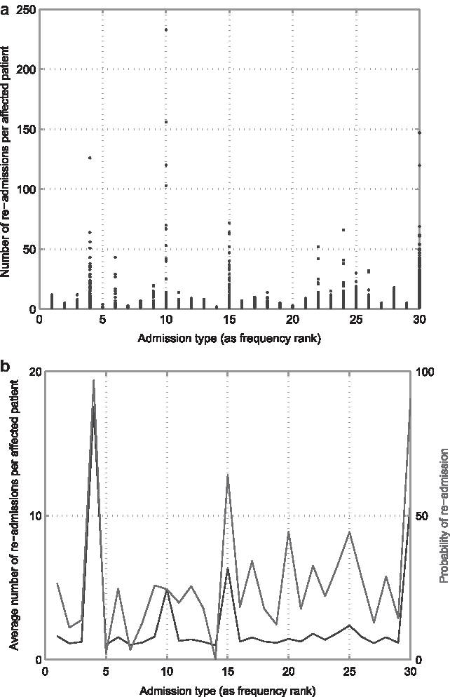
Frequency (red line) and cumulative frequency of different diagnoses. The plot illustrates the highly uneven distribution, with the top 30 most frequent diagnoses accounting for 75% of the entire data corpus.

A conceptual illustration of the method is shown in Figure 3.

FIG. 3.

Conceptual illustration of the method proposed by Arandjelović (2015b), which superimposes a Markovian model over a space of history vectors used to represent the medical state of a patient.

2.4. Limitations and questions

One of our contributions of this work is in the form of an analysis that scrutinizes the expectation that the method would scale well. In the original work (Arandjelović, 2015b), it was argued that the predictive performance of the method, reported with explicit modeling of the 30 most frequent diagnosis types only, could be maintained as a greater number of diagnosis types is included in the model as most practical applications would demand. The original article did not investigate this; rather, the number of salient, explicitly modeled diagnoses was set in an ad hoc manner to 30, explaining ∼75% of the data corpus (Arandjelović, 2015b). If our expectation of performance deterioration with an increased number of explicitly modeled diagnoses is correct, and if the rate of deterioration is high, the model could end up being of little practical significance: on the one end of the parameter spectrum, the model would provide high accuracy but insufficient specificity for its predictions to be practically useful, and on the other, the model would provide high specificity but poor accuracy for its predictions to be relied upon. Thus an analysis of this aspect of the original method is necessary before any practical use can be considered; our experiments as regards this issue are presented in Section 4.3.

3. Further Technical Contributions

In this section, we introduce our two main technical contributions. Our third contribution in the form of novel analyses and empirical results that highlight important and promising future research directions is presented in Section 4.

3.1. Improving the specificity of the model

The first major contribution of this work goes to the very heart of the learning framework underlying the diagnostic progression model, and concerns the issue of the space over which learning is performed. In other words, we propose a paradigm change in terms of what is explicitly learnt.

Recall from the previous section that the method described by Arandjelović (2015b) learns the probabilities of transitions from the space of history vectors to the same space of history vectors, that is, it learns \documentclass{aastex}\usepackage{amsbsy}\usepackage{amsfonts}\usepackage{amssymb}\usepackage{bm}\usepackage{mathrsfs}\usepackage{pifont}\usepackage{stmaryrd}\usepackage{textcomp}\usepackage{portland, xspace}\usepackage{amsmath, amsxtra}\usepackage{upgreek}\pagestyle{empty}\DeclareMathSizes{10}{9}{7}{6}\begin{document} $$p ( H ^{\prime} \vert H )$$ \end{document} , where H is a patient history vector and H a possible extension to that history, \documentclass{aastex}\usepackage{amsbsy}\usepackage{amsfonts}\usepackage{amssymb}\usepackage{bm}\usepackage{mathrsfs}\usepackage{pifont}\usepackage{stmaryrd}\usepackage{textcomp}\usepackage{portland, xspace}\usepackage{amsmath, amsxtra}\usepackage{upgreek}\pagestyle{empty}\DeclareMathSizes{10}{9}{7}{6}\begin{document} $$H ^{\prime} = H \to d$$ \end{document} . This approach naturally follows from the structure of the problem: both H and \documentclass{aastex}\usepackage{amsbsy}\usepackage{amsfonts}\usepackage{amssymb}\usepackage{bm}\usepackage{mathrsfs}\usepackage{pifont}\usepackage{stmaryrd}\usepackage{textcomp}\usepackage{portland, xspace}\usepackage{amsmath, amsxtra}\usepackage{upgreek}\pagestyle{empty}\DeclareMathSizes{10}{9}{7}{6}\begin{document} $$H ^{\prime}$$ \end{document} are states in a Markov chain and indeed the baseline formulation of this class of problems learns among other things precisely these transition probabilities. However, the very aspect of the history vector representation that makes it a powerful feature for longitudinal pattern extraction, in this instance introduces a significant practical limitation. Because history vectors are binarized, in general, a specific transition does not uniquely determine the diagnosis that caused the transition to occur. In particular, this occurs when a diagnosis already recorded in a patient's history is repeated—the transition from H to itself does not allow the method to distinguish between different diagnoses in the patient's history and determine which effected the transition (Vasiljeva and Arandjelović, 2016b). This is a major limitation given that many of the most serious diseases tend to be chronic in nature.

The method introduced in this article solves the described problem by changing the space over which learning is performed. In particular, rather than learning the probabilities of transitions between history vectors themselves, we learn the probabilities of follow-up diagnoses directly. It can be readily seen that this is a stronger learning task in the sense that knowing the follow-up diagnosis d allows for the computation of the next Markov chain state \documentclass{aastex}\usepackage{amsbsy}\usepackage{amsfonts}\usepackage{amssymb}\usepackage{bm}\usepackage{mathrsfs}\usepackage{pifont}\usepackage{stmaryrd}\usepackage{textcomp}\usepackage{portland, xspace}\usepackage{amsmath, amsxtra}\usepackage{upgreek}\pagestyle{empty}\DeclareMathSizes{10}{9}{7}{6}\begin{document} $$H ^{\prime} = H \to d$$ \end{document} without ambiguity, whereas the opposite is not the case, as described previously. What makes this learning choice particularly sensible is that it does not carry the burden of either greater computational complexity or learning challenge—the dimensionality of the space over which learning is performed stays exactly the same (it is governed by the choice of the number of salient diagnoses), which remains as densely populated as before. Hence, this learning paradigm change is unambiguously superior to that described originally.

3.2. Risk-driven inference

Our second key technical novelty concerns a major challenge in the development of models underlain by data from EHRs, which emerges from the pervasive problem known as the semantic gap (Vasiljeva and Arandjelović, 2016c). In colloquial terms, the problem is readily understood as arising from the lack of understanding of, say, disease etiology and physiology that an automatic method has in the interpretation of data from EHRs. For example, a human expert (such as a general practitioner or a specialist) who does have such knowledge may be readily able to discount even the consideration of certain disease interactions, which may be difficult to infer using a purely data-driven approach that machine methods generally employ. To overcome this challenge, some means of interaction, that is, information provision between an expert and a computer algorithm are needed. Yet, this interaction has to be intuitive and requires little effort and computing expertise.

The original authors correctly point out and thereafter empirically demonstrate that a major limitation in the use of Markovian models lies in their “forgetfulness.” This feature seemingly makes them inappropriate for the modeling under consideration here. They overcome this limitation by incorporating memory into the state representation itself. In particular, they describe what they term a history vector, which is a representation of a patient's diagnostic history in the form of a binary vector that encodes the types of diagnoses that the patient has been given in the past.

3.2.1. Identifying confounding factors

Consider two history vectors, H_x and H_y, which differ in the presence of only a single past diagnosis d_d. In other words, all bits in H_x and H_y are the same except for exactly one. A specific follow-up diagnosis d_f causes the transition of H_x and H_y to, respectively, \documentclass{aastex}\usepackage{amsbsy}\usepackage{amsfonts}\usepackage{amssymb}\usepackage{bm}\usepackage{mathrsfs}\usepackage{pifont}\usepackage{stmaryrd}\usepackage{textcomp}\usepackage{portland, xspace}\usepackage{amsmath, amsxtra}\usepackage{upgreek}\pagestyle{empty}\DeclareMathSizes{10}{9}{7}{6}\begin{document} $${H ^{\prime} _x}$$ \end{document} and \documentclass{aastex}\usepackage{amsbsy}\usepackage{amsfonts}\usepackage{amssymb}\usepackage{bm}\usepackage{mathrsfs}\usepackage{pifont}\usepackage{stmaryrd}\usepackage{textcomp}\usepackage{portland, xspace}\usepackage{amsmath, amsxtra}\usepackage{upgreek}\pagestyle{empty}\DeclareMathSizes{10}{9}{7}{6}\begin{document} $${H ^{\prime} _y}$$ \end{document} . We show how it can be automatically inferred if the differential diagnosis between h_x and h_y is one that affects the probability of d_f. We achieve this by using a Bayesian approach that readily lends itself to asymmetrical risk-driven inference, as described next. If the probability of d_f is not affected by the presence of d_d (in the context of other historical diagnoses in H_x and H_y, of course), then the transition data from the database of EHRs can be merged and thus used to estimate the aforesaid probability with higher precision, so clearly this is a highly desirable goal that can be used to reduce the amount of confounding factors greatly and improve the accuracy of the learnt models.

Consider what happens if H_x and H_y are indeed merged in the context of the prediction of d_f. In such a case, the number of observed transitions from H_x to \documentclass{aastex}\usepackage{amsbsy}\usepackage{amsfonts}\usepackage{amssymb}\usepackage{bm}\usepackage{mathrsfs}\usepackage{pifont}\usepackage{stmaryrd}\usepackage{textcomp}\usepackage{portland, xspace}\usepackage{amsmath, amsxtra}\usepackage{upgreek}\pagestyle{empty}\DeclareMathSizes{10}{9}{7}{6}\begin{document} $${H_x} \to {d_f}$$ \end{document} and those from H_y to \documentclass{aastex}\usepackage{amsbsy}\usepackage{amsfonts}\usepackage{amssymb}\usepackage{bm}\usepackage{mathrsfs}\usepackage{pifont}\usepackage{stmaryrd}\usepackage{textcomp}\usepackage{portland, xspace}\usepackage{amsmath, amsxtra}\usepackage{upgreek}\pagestyle{empty}\DeclareMathSizes{10}{9}{7}{6}\begin{document} $${H_y} \to {d_f}$$ \end{document} are considered as equivalent. By considering them jointly, a new probability of d_f from either H_x or H_y can be estimated. Let this probability be z. The total risk \documentclass{aastex}\usepackage{amsbsy}\usepackage{amsfonts}\usepackage{amssymb}\usepackage{bm}\usepackage{mathrsfs}\usepackage{pifont}\usepackage{stmaryrd}\usepackage{textcomp}\usepackage{portland, xspace}\usepackage{amsmath, amsxtra}\usepackage{upgreek}\pagestyle{empty}\DeclareMathSizes{10}{9}{7}{6}\begin{document} $$\rho$$ \end{document} of the aforesaid merger can then be computed as a sum of risks associated with the actual probabilities of d_f following H_x and H_y, respectively: \documentclass{aastex}\usepackage{amsbsy}\usepackage{amsfonts}\usepackage{amssymb}\usepackage{bm}\usepackage{mathrsfs}\usepackage{pifont}\usepackage{stmaryrd}\usepackage{textcomp}\usepackage{portland, xspace}\usepackage{amsmath, amsxtra}\usepackage{upgreek}\pagestyle{empty}\DeclareMathSizes{10}{9}{7}{6}\begin{document} \begin{align*} \rho = { \rho _x} + { \rho _y}. \tag{8} \end{align*} \end{document}

This risk emerges as a consequence of the fact that the empirical nature of EHRs inherently involves a degree of stochasticity, which means that there can never be absolute certainty that d_d is indeed entirely inconsequential in the context of this prediction. Instead, employing Bayesian framework, it is necessary to integrate over the latent probability of d_f following H_x and H_y and weigh this with the associated relative risk. In this manner for \documentclass{aastex}\usepackage{amsbsy}\usepackage{amsfonts}\usepackage{amssymb}\usepackage{bm}\usepackage{mathrsfs}\usepackage{pifont}\usepackage{stmaryrd}\usepackage{textcomp}\usepackage{portland, xspace}\usepackage{amsmath, amsxtra}\usepackage{upgreek}\pagestyle{empty}\DeclareMathSizes{10}{9}{7}{6}\begin{document} $${ \rho _x}$$ \end{document} , the risk can be written as: \documentclass{aastex}\usepackage{amsbsy}\usepackage{amsfonts}\usepackage{amssymb}\usepackage{bm}\usepackage{mathrsfs}\usepackage{pifont}\usepackage{stmaryrd}\usepackage{textcomp}\usepackage{portland, xspace}\usepackage{amsmath, amsxtra}\usepackage{upgreek}\pagestyle{empty}\DeclareMathSizes{10}{9}{7}{6}\begin{document} \begin{align*} { \rho _x} = {C_x} \int_z^1 \vert x - z \vert p ( x \vert {n_x} ) dx + \tag{9} \end{align*} \end{document} \documentclass{aastex}\usepackage{amsbsy}\usepackage{amsfonts}\usepackage{amssymb}\usepackage{bm}\usepackage{mathrsfs}\usepackage{pifont}\usepackage{stmaryrd}\usepackage{textcomp}\usepackage{portland, xspace}\usepackage{amsmath, amsxtra}\usepackage{upgreek}\pagestyle{empty}\DeclareMathSizes{10}{9}{7}{6}\begin{document} \begin{align*} \quad + ( 1 - {C_x} ) \int_0^z \vert z - x \vert p ( x \vert {n_x} ) dx. \tag{10} \end{align*} \end{document}

What this expression captures can be readily understood as follows. The first term quantifies the risk of z underestimating the true probability x of d_f following H_x (hence the integration is for \documentclass{aastex}\usepackage{amsbsy}\usepackage{amsfonts}\usepackage{amssymb}\usepackage{bm}\usepackage{mathrsfs}\usepackage{pifont}\usepackage{stmaryrd}\usepackage{textcomp}\usepackage{portland, xspace}\usepackage{amsmath, amsxtra}\usepackage{upgreek}\pagestyle{empty}\DeclareMathSizes{10}{9}{7}{6}\begin{document} $$x > z$$ \end{document} ). Similarly the second term quantifies the risk of z overestimating the true probability x of d_f following H_x (hence the integration is for \documentclass{aastex}\usepackage{amsbsy}\usepackage{amsfonts}\usepackage{amssymb}\usepackage{bm}\usepackage{mathrsfs}\usepackage{pifont}\usepackage{stmaryrd}\usepackage{textcomp}\usepackage{portland, xspace}\usepackage{amsmath, amsxtra}\usepackage{upgreek}\pagestyle{empty}\DeclareMathSizes{10}{9}{7}{6}\begin{document} $$x < z$$ \end{document} ). The two risks are in general weighted asymmetrically, as governed by the constant \documentclass{aastex}\usepackage{amsbsy}\usepackage{amsfonts}\usepackage{amssymb}\usepackage{bm}\usepackage{mathrsfs}\usepackage{pifont}\usepackage{stmaryrd}\usepackage{textcomp}\usepackage{portland, xspace}\usepackage{amsmath, amsxtra}\usepackage{upgreek}\pagestyle{empty}\DeclareMathSizes{10}{9}{7}{6}\begin{document} $${C_x} \in [ 0 , 1 ]$$ \end{document} , which should be set by a relevant medical professional. The aforesaid asymmetry captures what are in general different “costs” of overestimating and underestimating the probability of a particular diagnosis. For example, the cost of underestimating the probability of a terminal diagnosis is much greater than that of overestimating it by the same amount. In this case, C_x should be large, that is, closer to 1.

Continuing from Equation (9), using Bayes theorem, the term \documentclass{aastex}\usepackage{amsbsy}\usepackage{amsfonts}\usepackage{amssymb}\usepackage{bm}\usepackage{mathrsfs}\usepackage{pifont}\usepackage{stmaryrd}\usepackage{textcomp}\usepackage{portland, xspace}\usepackage{amsmath, amsxtra}\usepackage{upgreek}\pagestyle{empty}\DeclareMathSizes{10}{9}{7}{6}\begin{document} $$p ( x \vert {n_x} )$$ \end{document} can be rewritten as follows: \documentclass{aastex}\usepackage{amsbsy}\usepackage{amsfonts}\usepackage{amssymb}\usepackage{bm}\usepackage{mathrsfs}\usepackage{pifont}\usepackage{stmaryrd}\usepackage{textcomp}\usepackage{portland, xspace}\usepackage{amsmath, amsxtra}\usepackage{upgreek}\pagestyle{empty}\DeclareMathSizes{10}{9}{7}{6}\begin{document} \begin{align*} p ( x \vert { n_x } ) = { \frac { p ( { n_x } \vert x ) p ( x ) } { p ( { n_x } ) } } , \tag { 11 } \end{align*} \end{document}

where n_x is the number of cases in which d_f was the next diagnosis following H_x of the total of N_x transitions present in the EHRs database. Since the method has no means of establishing an informative prior on the transition probability x, an uninformative prior \documentclass{aastex}\usepackage{amsbsy}\usepackage{amsfonts}\usepackage{amssymb}\usepackage{bm}\usepackage{mathrsfs}\usepackage{pifont}\usepackage{stmaryrd}\usepackage{textcomp}\usepackage{portland, xspace}\usepackage{amsmath, amsxtra}\usepackage{upgreek}\pagestyle{empty}\DeclareMathSizes{10}{9}{7}{6}\begin{document} $$p ( x )$$ \end{document} is used, which leads to \documentclass{aastex}\usepackage{amsbsy}\usepackage{amsfonts}\usepackage{amssymb}\usepackage{bm}\usepackage{mathrsfs}\usepackage{pifont}\usepackage{stmaryrd}\usepackage{textcomp}\usepackage{portland, xspace}\usepackage{amsmath, amsxtra}\usepackage{upgreek}\pagestyle{empty}\DeclareMathSizes{10}{9}{7}{6}\begin{document} $$p ( x ) = 1$$ \end{document} since \documentclass{aastex}\usepackage{amsbsy}\usepackage{amsfonts}\usepackage{amssymb}\usepackage{bm}\usepackage{mathrsfs}\usepackage{pifont}\usepackage{stmaryrd}\usepackage{textcomp}\usepackage{portland, xspace}\usepackage{amsmath, amsxtra}\usepackage{upgreek}\pagestyle{empty}\DeclareMathSizes{10}{9}{7}{6}\begin{document} $$x \in [ 0 , 1 ]$$ \end{document} . Moreover, \documentclass{aastex}\usepackage{amsbsy}\usepackage{amsfonts}\usepackage{amssymb}\usepackage{bm}\usepackage{mathrsfs}\usepackage{pifont}\usepackage{stmaryrd}\usepackage{textcomp}\usepackage{portland, xspace}\usepackage{amsmath, amsxtra}\usepackage{upgreek}\pagestyle{empty}\DeclareMathSizes{10}{9}{7}{6}\begin{document} $$p ( {n_x} \vert x )$$ \end{document} is readily identifiable as a binomial distribution with parameter x and the number of draws N_x allowing \documentclass{aastex}\usepackage{amsbsy}\usepackage{amsfonts}\usepackage{amssymb}\usepackage{bm}\usepackage{mathrsfs}\usepackage{pifont}\usepackage{stmaryrd}\usepackage{textcomp}\usepackage{portland, xspace}\usepackage{amsmath, amsxtra}\usepackage{upgreek}\pagestyle{empty}\DeclareMathSizes{10}{9}{7}{6}\begin{document} $$p ( x \vert {n_x} )$$ \end{document} to be expanded further as follows: \documentclass{aastex}\usepackage{amsbsy}\usepackage{amsfonts}\usepackage{amssymb}\usepackage{bm}\usepackage{mathrsfs}\usepackage{pifont}\usepackage{stmaryrd}\usepackage{textcomp}\usepackage{portland, xspace}\usepackage{amsmath, amsxtra}\usepackage{upgreek}\pagestyle{empty}\DeclareMathSizes{10}{9}{7}{6}\begin{document} \begin{align*} p ( x \vert { n_x } ) = { \frac { p ( { n_x } \vert x ) } { p ( { n_x } ) } } \tag { 12 } \end{align*} \end{document} \documentclass{aastex}\usepackage{amsbsy}\usepackage{amsfonts}\usepackage{amssymb}\usepackage{bm}\usepackage{mathrsfs}\usepackage{pifont}\usepackage{stmaryrd}\usepackage{textcomp}\usepackage{portland, xspace}\usepackage{amsmath, amsxtra}\usepackage{upgreek}\pagestyle{empty}\DeclareMathSizes{10}{9}{7}{6}\begin{document} \begin{align*} \quad = { \frac { \left( { \begin{matrix} { { N_x } } \\ { { n_x } } \\ \end{matrix} } \right) { x^ { { n_x } } } { { ( 1 - x ) } ^ { { N_x } - { n_x } } } } { \int_0^1 p ( { n_x } \vert w ) dw } } \tag { 13 } \end{align*} \end{document} \documentclass{aastex}\usepackage{amsbsy}\usepackage{amsfonts}\usepackage{amssymb}\usepackage{bm}\usepackage{mathrsfs}\usepackage{pifont}\usepackage{stmaryrd}\usepackage{textcomp}\usepackage{portland, xspace}\usepackage{amsmath, amsxtra}\usepackage{upgreek}\pagestyle{empty}\DeclareMathSizes{10}{9}{7}{6}\begin{document} \begin{align*} \quad \quad \quad \quad = { \frac { { x^ { { n_x } } } { { ( 1 - x ) } ^ { { N_x } - { n_x } } } } { \int_0^1 \left( { \begin {matrix} { { N_x } } \\ { { n_x } } \\ \end {matrix} } \right) { w^ { { n_x } } } { { ( 1 - w ) } ^ { { N_x } - { n_x } } } dw } } \tag { 14 } \end{align*} \end{document} \documentclass{aastex}\usepackage{amsbsy}\usepackage{amsfonts}\usepackage{amssymb}\usepackage{bm}\usepackage{mathrsfs}\usepackage{pifont}\usepackage{stmaryrd}\usepackage{textcomp}\usepackage{portland, xspace}\usepackage{amsmath, amsxtra}\usepackage{upgreek}\pagestyle{empty}\DeclareMathSizes{10}{9}{7}{6}\begin{document} \begin{align*} \quad \quad \quad \quad = { \frac { { x^ { { n_x } } } { { ( 1 - x ) } ^ { { N_x } - { n_x } } } } { \left( { \begin {matrix} { { N_x } } \\ { { n_x } } \\ \end {matrix} } \right) \beta ( { n_x } + 1 , { N_x } - { n_x } + 1 ) } } , \tag { 15 } \end{align*} \end{document}

where \documentclass{aastex}\usepackage{amsbsy}\usepackage{amsfonts}\usepackage{amssymb}\usepackage{bm}\usepackage{mathrsfs}\usepackage{pifont}\usepackage{stmaryrd}\usepackage{textcomp}\usepackage{portland, xspace}\usepackage{amsmath, amsxtra}\usepackage{upgreek}\pagestyle{empty}\DeclareMathSizes{10}{9}{7}{6}\begin{document} $$\beta ( \cdot )$$ \end{document} is the Euler beta function, and simple marginalization over x is performed in the denominator. This expression can be substituted back into Equations (9) and (10), and then Equation (8), and the integration performed numerically [which is both simple and fast, given that it is a simple integration in one dimension (1D)].

Notes and remarks on practical application: It is insightful to highlight several important practical aspects of the proposed technique. First, once implemented as software, it is intuitive to use—the tradeoff between overdiagnosis and underdiagnosis is a concept routinely dealt with by medical professionals, and it is simply set using a single constant that balances the two risks. The risk is also readily interpretable. For example, for a terminal diagnosis the integrand in Equation (9) can be interpreted as computing the number of individuals who would be incorrectly expected to have a terminal diagnosis—an undesirable mistake considering the potential emotional stress, to begin with. Similarly, for a terminal diagnosis, the integrand in Equation (10) estimates the number of individuals who would experience a terminal episode that would not be predicted—arguably an even more serious mistake in that it ipso facto involves the loss of life. The acceptable tradeoff can be made by a clinician either on the level of an individual patient, for a specific diagnosis, or for an entire class of diagnoses (e.g., the same baseline risk tradeoff could be set for an entire ICD chapter, such as chapter IX that covers circulatory system diseases). In summary, the proposed technique is simple and intuitive to use, and it allows a high degree of flexibility in the choice of specificity or generality in application.

4. Evaluation

In this section, we summarize some of the experiments we conducted to evaluate the proposed framework and derive useful insights that illuminate possible avenues for improvement and future work.

4.1. EHR data

In an effort to reduce the possibility of introducing variability because of confounding variables, we sought to standardize our evaluation protocol as much as possible with that adopted by previous work. Hence, we requested access to the large collection of EHRs described by Arandjelović (2015b) and were kindly provided 75% of the records used in the aforementioned article. For completeness, here we summarize the key features of this subset.

The EHRs adopted for evaluation were collected by a large private hospital in Fife, Scotland. The distribution of patient age in the database is \documentclass{aastex}\usepackage{amsbsy}\usepackage{amsfonts}\usepackage{amssymb}\usepackage{bm}\usepackage{mathrsfs}\usepackage{pifont}\usepackage{stmaryrd}\usepackage{textcomp}\usepackage{portland, xspace}\usepackage{amsmath, amsxtra}\usepackage{upgreek}\pagestyle{empty}\DeclareMathSizes{10}{9}{7}{6}\begin{document} $$75 \pm 14$$ \end{document} years, the youngest and oldest patients being 18 months and 105 years old, respectively, with the male to female ratio being \documentclass{aastex}\usepackage{amsbsy}\usepackage{amsfonts}\usepackage{amssymb}\usepackage{bm}\usepackage{mathrsfs}\usepackage{pifont}\usepackage{stmaryrd}\usepackage{textcomp}\usepackage{portland, xspace}\usepackage{amsmath, amsxtra}\usepackage{upgreek}\pagestyle{empty}\DeclareMathSizes{10}{9}{7}{6}\begin{document} $$56:44$$ \end{document} . Approximately 23% of the patients in the database have a date of death associated with their EHR, which means that they are deceased and thus have a record of a terminal diagnosis. The entire EHR collection spans a period of 10 years, with the average number of diagnoses per patient of \documentclass{aastex}\usepackage{amsbsy}\usepackage{amsfonts}\usepackage{amssymb}\usepackage{bm}\usepackage{mathrsfs}\usepackage{pifont}\usepackage{stmaryrd}\usepackage{textcomp}\usepackage{portland, xspace}\usepackage{amsmath, amsxtra}\usepackage{upgreek}\pagestyle{empty}\DeclareMathSizes{10}{9}{7}{6}\begin{document} $$9.9 \pm 64.0$$ \end{document} .

4.2. Baseline model validation

Interestingly, on our data set, the patient's age was found not to be associated with the number of admissions on record, whereas a low positive correlation \documentclass{aastex}\usepackage{amsbsy}\usepackage{amsfonts}\usepackage{amssymb}\usepackage{bm}\usepackage{mathrsfs}\usepackage{pifont}\usepackage{stmaryrd}\usepackage{textcomp}\usepackage{portland, xspace}\usepackage{amsmath, amsxtra}\usepackage{upgreek}\pagestyle{empty}\DeclareMathSizes{10}{9}{7}{6}\begin{document} $$( r = 0.14 )$$ \end{document} was found between the patient's age and the number of conditions the patient had been diagnosed with at some point in the past—see Figure 4a and b. A better predictor of the number of admissions was found to be the presence of a particular diagnosis (e.g., a high number of admissions are associated with the presence of the diagnoses of mental disorders, renal, and cardiovascular conditions), as illustrated in Figure 5a and b. Further insight can be gained by examining Figure 6a and b, which summarize the repeated diagnosis statistics across different conditions. A mental disorder diagnosis or dialysis treatment, for example, predicts both a high probability of a repeated diagnosis and a high total number of the diagnosis type on record. These results are consistent with previous studies in the literature (Allaudeen et al., 2011; Kilkenny et al., 2013; Vigod et al., 2013) and support our diagnosis presence-based model.

FIG. 4.

(a) Patient age is not associated with the total number of admissions of the patient. (b) Patient age shows low association \documentclass{aastex}\usepackage{amsbsy}\usepackage{amsfonts}\usepackage{amssymb}\usepackage{bm}\usepackage{mathrsfs}\usepackage{pifont}\usepackage{stmaryrd}\usepackage{textcomp}\usepackage{portland, xspace}\usepackage{amsmath, amsxtra}\usepackage{upgreek}\pagestyle{empty}\DeclareMathSizes{10}{9}{7}{6}\begin{document} $$( r = 0.14 , p < 0.001 )$$ \end{document} with the number of conditions the patient has been diagnosed with.

FIG. 5.

(a) The presence of a particular condition in a patient's history is a good predictor of the total number admissions. (b) Average number of admissions for patients containing a particular diagnosed condition in their history.

FIG. 6.

(a) Repeated diagnosis statistics for the top 30 diagnosed conditions. (b) Average number of repeated admissions and the probability of a repeated diagnosis for a particular condition.

4.2.1. Next diagnosis prediction

To evaluate the predictive power of the proposed model, we examined its performance in the prediction of the next diagnosis based on a patient's prior diagnosis history, and compared this with the performance of the Markov process-based approach described previously; see Equations (1)–(3). Both methods were trained using an 80–20 split of data into training and test. Specifically, 80% of the data corpus were used to learn the model parameters—conditional probabilities \documentclass{aastex}\usepackage{amsbsy}\usepackage{amsfonts}\usepackage{amssymb}\usepackage{bm}\usepackage{mathrsfs}\usepackage{pifont}\usepackage{stmaryrd}\usepackage{textcomp}\usepackage{portland, xspace}\usepackage{amsmath, amsxtra}\usepackage{upgreek}\pagestyle{empty}\DeclareMathSizes{10}{9}{7}{6}\begin{document} $$p ( \hat H \to d \vert \hat H )$$ \end{document} in the case of the proposed model and \documentclass{aastex}\usepackage{amsbsy}\usepackage{amsfonts}\usepackage{amssymb}\usepackage{bm}\usepackage{mathrsfs}\usepackage{pifont}\usepackage{stmaryrd}\usepackage{textcomp}\usepackage{portland, xspace}\usepackage{amsmath, amsxtra}\usepackage{upgreek}\pagestyle{empty}\DeclareMathSizes{10}{9}{7}{6}\begin{document} $$p ( d \to d ^{\prime} )$$ \end{document} for the Markov process-based model. The remaining 20% of the data were used as test input. For each test patient, we considered the predictions obtained by the two methods, given all possible partial histories. In other words, given a patient with the full diagnosis history \documentclass{aastex}\usepackage{amsbsy}\usepackage{amsfonts}\usepackage{amssymb}\usepackage{bm}\usepackage{mathrsfs}\usepackage{pifont}\usepackage{stmaryrd}\usepackage{textcomp}\usepackage{portland, xspace}\usepackage{amsmath, amsxtra}\usepackage{upgreek}\pagestyle{empty}\DeclareMathSizes{10}{9}{7}{6}\begin{document} $$H = {d_1} \to {d_2} \to \cdots \to {d_n}$$ \end{document} , we obtain predictions using partial histories \documentclass{aastex}\usepackage{amsbsy}\usepackage{amsfonts}\usepackage{amssymb}\usepackage{bm}\usepackage{mathrsfs}\usepackage{pifont}\usepackage{stmaryrd}\usepackage{textcomp}\usepackage{portland, xspace}\usepackage{amsmath, amsxtra}\usepackage{upgreek}\pagestyle{empty}\DeclareMathSizes{10}{9}{7}{6}\begin{document} $${H_k} = {d_1} \to \cdots \to {d_k}$$ \end{document} for \documentclass{aastex}\usepackage{amsbsy}\usepackage{amsfonts}\usepackage{amssymb}\usepackage{bm}\usepackage{mathrsfs}\usepackage{pifont}\usepackage{stmaryrd}\usepackage{textcomp}\usepackage{portland, xspace}\usepackage{amsmath, amsxtra}\usepackage{upgreek}\pagestyle{empty}\DeclareMathSizes{10}{9}{7}{6}\begin{document} $$k = 1 \ldots n - 1$$ \end{document} .

A summary of the results is given in Figure 7, which shows the cumulative match characteristic (CMC) curves corresponding to the two methods—each point on a curve represents the proportion of cases (ordinate) for which the actual correct diagnosis type is at worst predicted with a specific rank (abscissa). The first thing that is readily observed from the plot is that the proposed method (blue line) vastly outperforms the Markov process-based approach (red line). What is more, the accuracy of our method is rather remarkable—it correctly predicts the type of the next diagnosis for a patient in 82% of the cases (rank-1). Already at rank-2, the accuracy is nearly 90%. In comparison, the Markov process-based method achieves only 35% accuracy at rank-1, less than 50% at rank-2, and reaches 90% only at rank-17.

FIG. 7.

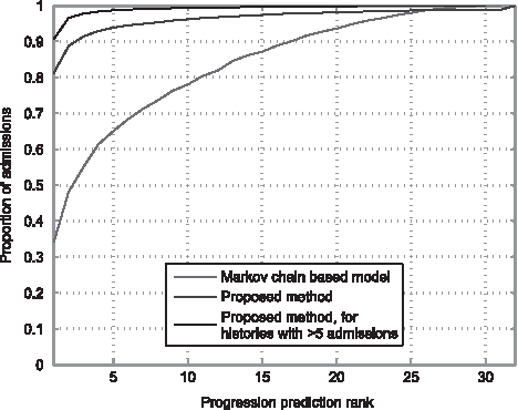
Cumulative match characteristics (CMCs) for the prediction of the next diagnosis from a patient's history.

It is interesting to observe a particular feature of the CMC plot for the proposed method. Notice its tail behavior—at rank-25 and higher, the Markov process-based approach catches up and actually performs better. Although performance at such a high rank is not of direct practical interest, it is insightful to consider how this observation can be explained, given that it is highly unlikely for it to be a mere statistical anomaly, considering the amount of data used to estimate the characteristics. The answer is readily revealed by considering the plot in Figure 8, which shows the dependency between the average rank of the proposed method's prediction and the length of the partial history used as input. Specifically, notice that higher ranks (i.e., worse performance) are associated with short histories. Put differently, when there is little information in a patient's history, there is more uncertainty about the patient's possible future ailments. This observation too strongly supports the validity of our model as it shows that accumulating evidence is used and represented in a more meaningful and robust way, which allows for the learning of complex interactions between conditions and their development. Finally, this is illustrated in Figure 7, which also shows the plot of the proposed method's CMC curve restricted to test histories containing at least five prior diagnoses. In this case, rank-1 and rank-2 performances reach the remarkable accuracy of 91% and 97%, respectively.

FIG. 8.

Partial history length versus next diagnosis prediction rank.

4.2.2. Long-term prediction

Given the outstanding performance of our method in predicting the type of the next diagnosis given the patient's current medical history, we next considered how the proposed model performs in long-term predictions. Considering that we are now dealing with sequences of future diagnoses and thus a much greater space of possible options, the characterization of performance using CMC curves is impractical. Rather, we now compare our approach with the Markov process-based method by using the corresponding conditional probabilities for the actual progression observed in the data. In other words, for the prediction following a partial history \documentclass{aastex}\usepackage{amsbsy}\usepackage{amsfonts}\usepackage{amssymb}\usepackage{bm}\usepackage{mathrsfs}\usepackage{pifont}\usepackage{stmaryrd}\usepackage{textcomp}\usepackage{portland, xspace}\usepackage{amsmath, amsxtra}\usepackage{upgreek}\pagestyle{empty}\DeclareMathSizes{10}{9}{7}{6}\begin{document} $$\hat H$$ \end{document} of the length k and the correct full history \documentclass{aastex}\usepackage{amsbsy}\usepackage{amsfonts}\usepackage{amssymb}\usepackage{bm}\usepackage{mathrsfs}\usepackage{pifont}\usepackage{stmaryrd}\usepackage{textcomp}\usepackage{portland, xspace}\usepackage{amsmath, amsxtra}\usepackage{upgreek}\pagestyle{empty}\DeclareMathSizes{10}{9}{7}{6}\begin{document} $$H = \hat H \to {d_{k + 1}} \to \cdots \to {d_n}$$ \end{document} , we compute the log ratio of conditional probabilities: \documentclass{aastex}\usepackage{amsbsy}\usepackage{amsfonts}\usepackage{amssymb}\usepackage{bm}\usepackage{mathrsfs}\usepackage{pifont}\usepackage{stmaryrd}\usepackage{textcomp}\usepackage{portland, xspace}\usepackage{amsmath, amsxtra}\usepackage{upgreek}\pagestyle{empty}\DeclareMathSizes{10}{9}{7}{6}\begin{document} \begin{align*} \rho = \log \left( { { \frac { { p_ { { \rm { Markov } } } } ( \hat H \to { d_ { k + 1 } } \to \cdots \to { d_n } \vert \hat H ) } { { p_ { { \rm { proposed } } } } ( \hat H \to { d_ { k + 1 } } \to \cdots \to { d_n } \vert \hat H ) } } } \right). \tag { 16 } \end{align*} \end{document}

A positive value of \documentclass{aastex}\usepackage{amsbsy}\usepackage{amsfonts}\usepackage{amssymb}\usepackage{bm}\usepackage{mathrsfs}\usepackage{pifont}\usepackage{stmaryrd}\usepackage{textcomp}\usepackage{portland, xspace}\usepackage{amsmath, amsxtra}\usepackage{upgreek}\pagestyle{empty}\DeclareMathSizes{10}{9}{7}{6}\begin{document} $$\rho$$ \end{document} means that the Markov process-based method performed better and a negative value than the proposed method did. The greater the absolute value of \documentclass{aastex}\usepackage{amsbsy}\usepackage{amsfonts}\usepackage{amssymb}\usepackage{bm}\usepackage{mathrsfs}\usepackage{pifont}\usepackage{stmaryrd}\usepackage{textcomp}\usepackage{portland, xspace}\usepackage{amsmath, amsxtra}\usepackage{upgreek}\pagestyle{empty}\DeclareMathSizes{10}{9}{7}{6}\begin{document} $$\rho$$ \end{document} the greater is the measured difference in performance in the corresponding direction. As before, we divide the data into training and test sets using an 80–20 split and consider the predictions for all possible partial histories in the test set.

A summary of the results is presented in Figure 9. Specifically, the plot shows the cumulative distribution function (CDF) of the log ratio \documentclass{aastex}\usepackage{amsbsy}\usepackage{amsfonts}\usepackage{amssymb}\usepackage{bm}\usepackage{mathrsfs}\usepackage{pifont}\usepackage{stmaryrd}\usepackage{textcomp}\usepackage{portland, xspace}\usepackage{amsmath, amsxtra}\usepackage{upgreek}\pagestyle{empty}\DeclareMathSizes{10}{9}{7}{6}\begin{document} $$\rho$$ \end{document} . As in the case of the one-step prediction, it is readily apparent that the performance of the proposed method vastly exceeds that of the Markov process-based approach. The value of CDF at the crossing of the curve with the \documentclass{aastex}\usepackage{amsbsy}\usepackage{amsfonts}\usepackage{amssymb}\usepackage{bm}\usepackage{mathrsfs}\usepackage{pifont}\usepackage{stmaryrd}\usepackage{textcomp}\usepackage{portland, xspace}\usepackage{amsmath, amsxtra}\usepackage{upgreek}\pagestyle{empty}\DeclareMathSizes{10}{9}{7}{6}\begin{document} $$\rho = 0$$ \end{document} line is 0.82, which means that our method exhibited superior performance in 82% of the predictions. Even in the case of 18% of the predictions in which the Markov process-based method performed better, the performance differential is not substantial. This is in sharp contrast with the instances in which the proposed method was better—in 67% of the cases, the conditional probability of the correct history progression was more than 100 greater for our model.

FIG. 9.

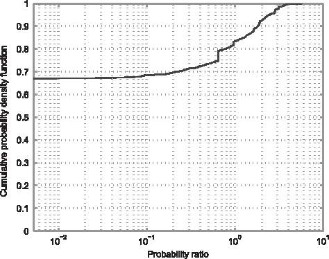
Cumulative density function of the ratio of the probabilities of true patient medical history progression for the diagnoses-level Markov process approach and the proposed method.

4.3. Assessing model scalability

Our primary goal here is to examine how the predictive performance of the history vector-based model is affected by the choice of the number of salient diagnostic codes (Vasiljeva and Arandjelović, 2016a). As in Arandjelović (2015b), we too assess the quality of a specific prediction by considering the rank of the ground truth diagnostic code in the probability ordered list of predictions. Formally, let d_t be the ground truth diagnostic code that follows a particular history H. Then the rank r of d_t is given by the number of diagnostic codes that the model predicts as following H with at least the probability \documentclass{aastex}\usepackage{amsbsy}\usepackage{amsfonts}\usepackage{amssymb}\usepackage{bm}\usepackage{mathrsfs}\usepackage{pifont}\usepackage{stmaryrd}\usepackage{textcomp}\usepackage{portland, xspace}\usepackage{amsmath, amsxtra}\usepackage{upgreek}\pagestyle{empty}\DeclareMathSizes{10}{9}{7}{6}\begin{document} $$p ( H \to {d_t} )$$ \end{document} : \documentclass{aastex}\usepackage{amsbsy}\usepackage{amsfonts}\usepackage{amssymb}\usepackage{bm}\usepackage{mathrsfs}\usepackage{pifont}\usepackage{stmaryrd}\usepackage{textcomp}\usepackage{portland, xspace}\usepackage{amsmath, amsxtra}\usepackage{upgreek}\pagestyle{empty}\DeclareMathSizes{10}{9}{7}{6}\begin{document} \begin{align*} r = \vert \left\{ {d:d \in D \wedge p ( H \to d ) \ge p ( H \to {d_t} ) } \right\} \vert. \tag{17} \end{align*} \end{document}

We used the same granularity of codes as the original work described in Arandjelović (2015b).

Furthermore, we adopt the usual “leave one out” evaluation protocol, whereby the performance of the method is tested with each patient's data in turn and the model trained using the data of all other patients. To quantify the aggregate performance of the model for specific model parameter values (i.e., the number of salient diagnoses included in the history vector representation), we use two well-known measures. These are the average rank (a special case of the average normalized rank (Salton and McGill, 1983) when the set of target matches is exactly equal to 1) and the normalized area under the CMC curve. For each possible rank r ( \documentclass{aastex}\usepackage{amsbsy}\usepackage{amsfonts}\usepackage{amssymb}\usepackage{bm}\usepackage{mathrsfs}\usepackage{pifont}\usepackage{stmaryrd}\usepackage{textcomp}\usepackage{portland, xspace}\usepackage{amsmath, amsxtra}\usepackage{upgreek}\pagestyle{empty}\DeclareMathSizes{10}{9}{7}{6}\begin{document} $$r = 1 \ldots n$$ \end{document} , where n is the worst possible rank, equal to the number of diagnosis types), the CMC takes on the value equal to the proportion of predictions that predict the correct diagnosis at worst with the rank r (Bolle et al., 2005). The ideal performance results in the CMC having the value 1 across all ranks, that is, in each individual case, the correct diagnosis is ranked 1. The area under the curve is normalized so that it is equal to 1 in this ideal case.

We started by looking at the effect that changing the number of salient diagnosis types, that is, diagnosis codes with the corresponding (1-to-1) elements in the history vector, has on the area under the CMC curve. Our experimental results are captured by the plot in Figure 10a. The plot can be readily seen to support our hypothesis that predicted a decay in the adopted model's prediction performance for an increasing number of explicitly modeled diagnoses. Notwithstanding this unwelcome qualitative observation, the major result is of a quantitative nature—the rate of the aforementioned decay is very slow indeed. Like many other natural phenomena, the decay exhibits a power law form with the associated exponent value, which differs from 1 by only 5 parts in 100,000, that is, it is equal to \documentclass{aastex}\usepackage{amsbsy}\usepackage{amsfonts}\usepackage{amssymb}\usepackage{bm}\usepackage{mathrsfs}\usepackage{pifont}\usepackage{stmaryrd}\usepackage{textcomp}\usepackage{portland, xspace}\usepackage{amsmath, amsxtra}\usepackage{upgreek}\pagestyle{empty}\DeclareMathSizes{10}{9}{7}{6}\begin{document} $$1 - 0.5 \times {10^{ - 5}}$$ \end{document} . The practical significance of this finding is better appreciated by considering the plot in Figure 10b. This plot shows the variation in the area under the CMC curve as a function of the coverage of the entire diagnosis data corpus by the salient codes. The outstanding performance of the adopted method is illustrated well by noting, for example, that the dimensionality of history vectors can be increased to explicitly model the number of most frequent diagnosis codes, which cover more than 91% of the data, with the predictive performance of the method dropping by a mere 0.5% as compared with the coverage of only 61%. Even 98% of data coverage results in a change of only 0.8%. Recall that in the original article, the authors used 30 codes that accounted for 75% of the diagnoses in the corpus. Our results demonstrate that this was an overly conservative value.

FIG. 10.

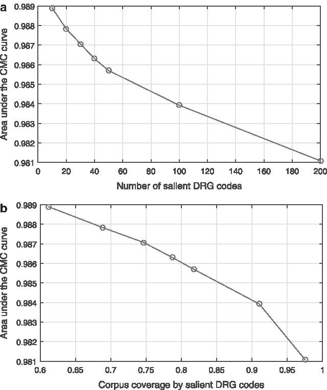
The normalized area under the CMC curve.

We next examined the average prediction rank of the correct diagnosis type, which offers further insight into the performance of the adopted method. As expected from the previous set of findings, the results summarized by the plots in Figure 11a and b corroborate the observation that an increase in the dimensionality of history vectors, a key parameter of the method, worsens performance. In this experiment, this worsening is exhibited as an increase in the average rank (i.e., a greater number of incorrect predictions are made with a higher probability than the actual ground truth diagnosis type). It is interesting to note the significance of what appears to be a much more rapid performance deterioration in terms of this performance measure in comparison with the area under the CMC curve discussed previously. For example, although the use of 200 versus 10 most frequent diagnosis codes effects a reduction of only 0.5% in the area under the CMC curve, the corresponding change in the average rank of the correct diagnosis type increases fivefold (from ∼1.5 for 10 salient codes to ∼7.3 for 200 salient codes). The explanation for this apparent discrepancy is in fact reassuring as it demonstrates that the most dramatic changes in the predicted rank happen for predictions that are already not very good, that is, the small number of bad predictions becomes even worse, rather than good predictions becoming bad.

FIG. 11.

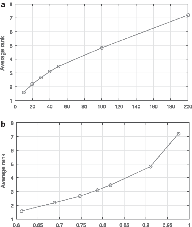
The average prediction rank of the correct diagnosis type.

Lastly, to examine in additional detail of how an increase in the number of explicitly modeled diagnosis types affects predictions, we looked at prediction rank histograms for different diagnosis codes and the corresponding changes as their number was changed. Figure 12a and b contrasts the histograms for 20 and 50 salient diagnosis types. It is remarkable to observe that in both cases the histograms are virtually identical across different codes within the same model. Rather than being effected by subpar histograms of the added codes, the (small, as demonstrated previously) deterioration in predictive performance as the number of salient diagnosis types is increased is effected by slightly worse predictive performance uniformly distributed across different diagnoses. This is highly preferable in practice as it implies that for a fixed model, complexity predictive power remains the same regardless of the patient's ailment. Were it otherwise, the predictions would be more difficult to interpret and the model complexity more challenging to set appropriately as the model's predictive performance would exhibit dependence on the nature of the health problems affecting a specific patient.

FIG. 12.

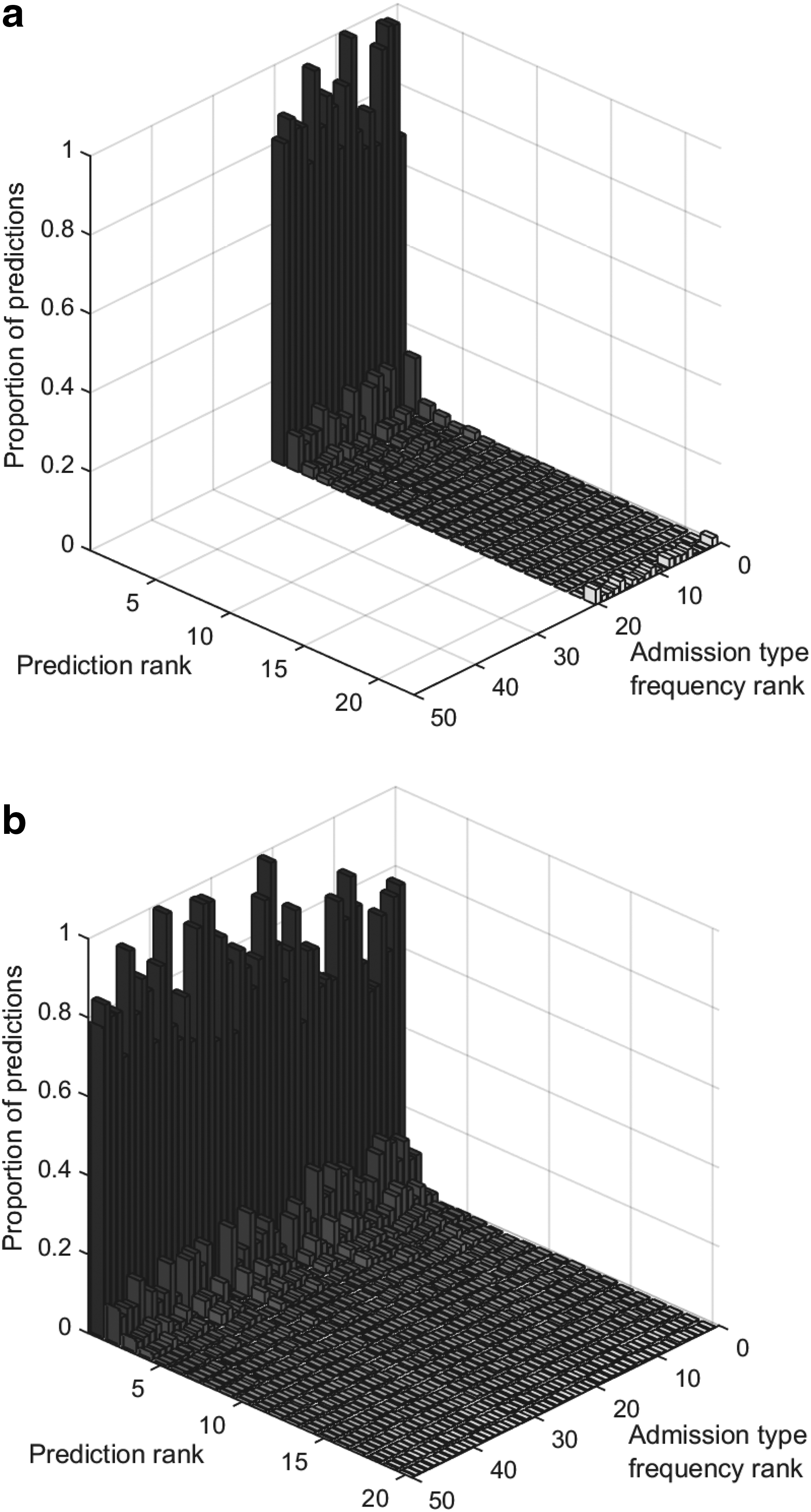
Prediction rank histograms across different diagnosis codes using (a) 20 versus (b) 50 salient codes.

4.3.1. Assessing the effects of incorporating explicit clinical knowledge

First, we examined how the number of transition merges changes with the variation in the values of the two free parameters, namely the merging threshold t_m and the relative risk weighting constant C_x in Equations (9) and (10). We applied our method to the entire EHRs data set, although, as noted in the previous section, in practice it is likely that different parameters would be applied to different subtrees of the diagnosis coding hierarchy.

Our findings are summarized by the surface plot shown in Figure 13. Although it is inherently the case that increasing t_m cannot reduce the number of merges made, the characteristics of the corresponding change are insightful to the clinician in that they can be used to guide the choice of the risk weighting constant. Notice, for example, that the number of effected merges increases approximately linearly across the entire range of t_m for C_x smaller than ∼0.5, whereas for C_x greater than 0.5, there is a much more sudden increase.

FIG. 13.

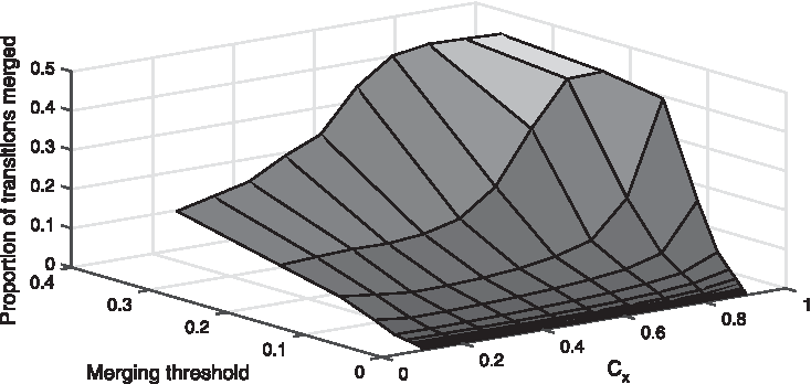
Surface plot showing the number of pair-wise merges performed (as the proportion of all possible transitions pairs that could possibly be merged) as a function of the adjustable parameters of the proposed method, namely the merging threshold t_m and the relative risk weighting constant C_x in Equations (9) and (10).

Next we examined salient diagnoses d_f (see Section 3.2) associated with the greatest number of merges. We noticed that the diagnosis of stroke was one of the particularly represented diagnosis among these, across different values of t_m and C_x, so we examined the corresponding merging behavior in more detail. Interpreted intuitively, this means that on average the diagnosis of stroke has the least effect on (from the set of salient diagnoses included in the history vector) the prognosis of other ailments. The family of curves for different values of C_x, showing the variation of the number of merges (as the proportion of all possible transitions pairs that could possibly be merged and associated with transitions effected by the diagnosis of stroke) as a function of the merging threshold t_m, is shown in Figure 14. It is insightful to observe that much like as shown in Figure 13, an increase in C_x results in more merges for the same value of t_m. A careful consideration of characteristics such as this one is crucial in the practical deployment of the proposed method, and the choice of granularity (in the context of the diagnosis coding hierarchy) at which the method is applied and its parameters.

FIG. 14.

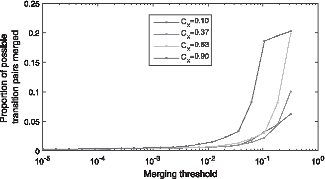
The number of effected merges associated with the diagnosis of stroke (as d_f in Section 3.2) as the proportion of all possible transitions pairs that could possibly be merged and associated with transitions effected by the diagnosis of stroke.

5. Summary and Future Work

In this article, we introduced a novel algorithm that uses machine learning on EHR collections for the discovery of longitudinal patterns in the diagnoses of diseases. The two key technical novelties are (i) a novel learning paradigm that enables greater learning specificity and (ii) a method for risk-driven identification of confounding diagnoses. A series of experiments were presented to demonstrate the effectiveness of the proposed techniques. Novel insights resulting from our experimental findings were also discussed and highlighted.

As regards possible future work directions, a number of possibilities were proposed by the authors of the original history vector-based approach that the present method was partly inspired by. Although we agree with most of these in broad terms, our contributions, experiments, and results suggest what we believe to be more promising immediate alternatives. In particular, although we agree with the authors of the original method that the presence of a particular episode of care is a predictive factor not much weaker than the exact number of episodes (which would require a prohibitively large amount of training data to learn), we believe that history vector binarization is an overly harsh step for the reduction of the learning space. Following the spirit of the method introduced in this article, we intend to explore the possibility of automatically detecting chronic types of episodes of care (dialysis, for example) and then using a binary representation for nonchronic and a more graded representation for chronic conditions.

Footnotes

Author Disclosure Statement

No competing financial interests exist.

References

Allaudeen

, Vidyarthi

, Maselli

, et al. 2011. Redefining readmission risk factors for general medicine patients. J. Hosp. Med. 6, 54–60.

Andrei

, and Arandjelović

2016. Identification of promising research directions using machine learning aided medical literature analysis. In Proc. International Conference of the IEEE Engineering in Medicine and Biology Society, 2471–2474. IEEE, Orlando, FL.

Arandjelović

2011. Contextually learnt detection of unusual motion-based behaviour in crowded public spaces. In Proc. International Symposium on Computer and Information Sciences, 403–410. Springer, London, UK.

Arandjelović

2015a. Prediction of health outcomes using big (health) data. In Proc. International Conference of the IEEE Engineering in Medicine and Biology Society, 2543–2546. IEEE, Milan, Italy.

Arandjelović

2015b. Modelling disease progression using electronic hospital records. In Proc. IJCAI Workshop on Bioinformatics and Artificial Intelligence, 10–16. AAAI, Buenos Aires, Argentina.

Arandjelović

2016. On the discovery of hospital admission patterns—A clarification. Bioinformatics, 32, 2078.

Barracliffe

, Arandjelović

, and Humphris

2017. Can machine learning predict healthcare professionals' responses to patient emotions? In Proc. International Conference on Bioinformatics and Computational Biology. ISCA, Honolulu, HI.

Bartolomeo

, Trerotoli

, Moretti

, et al. 2008. A Markov model to evaluate hospital readmission. BMC Med. Res. Methodol. 8, 23.

Berwick

D.M.

, and Hackbarth

A.D.

2012. Eliminating waste in US health care. JAMA, 307, 1513–1516.

10.

Bessou

, Guelfucci

, Aballea

, et al. 2015. Comparison of comorbidity measures to predict economic outcomes in a large UK primary care database. Value Health, 18, A691.

11.

Beykikhoshk

, Arandjelović

, Phung

, et al. 2014. Data-mining Twitter and the autism spectrum disorder: A pilot study. In Proc. IEEE/ACM International Conference on Advances in Social Network Analysis and Mining, 349–356. IEEE, Beijing, China.

12.

Beykikhoshk

, Arandjelović

, Phung

, et al. 2015a. Hierarchical Dirichlet process for tracking complex topical structure evolution and its application to autism research literature. In Proc. Pacific-Asia Conference on Knowledge Discovery and Data Mining, 1, 550–562. IEEE, Ho Chi Minh City, Viet Nam.

13.

Beykikhoshk

, Arandjelović

, Phung

, et al. 2015b. Using Twitter to learn about the autism community. Soc. Netw. Anal. Min. 5, 5–22. Springer.

14.

Beykikhoshk

, Phung

, Arandjelović

, et al. 2016. Analysing the history of autism spectrum disorder using topic models. In Proc. IEEE International Conference on Data Science and Advanced Analytics, 762–771. IEEE, Montreal, Canada.

15.

Bhatnagar

, Wickramasinghe

, Williams

, et al. 2015. The epidemiology of cardiovascular disease in the UK 2014. Heart, 101, 1182–1189.

16.

Birkhead

G.S.

, Klompas

, and Shah

N.R.

2015. Uses of electronic health records for public health surveillance to advance public health. Annu. Rev. Public Health, 36, 345–359.

17.

Bolle

R.M.

, Connell

J.H.

, Pankanti

, et al. 2005. The relation between the ROC curve and the CMC. In Proc. IEEE Workshop on Automatic Identification Advanced Technologies, 15–20. IEEE, Washington, USA.

18.

Butler

, and Kalogeropoulos

2012. Hospital strategies to reduce heart failure readmissions. J. Am. Coll. Cardiol. 60, 615–617.

19.

Canavan

, West

, and Card

2015. Calculating total health service utilisation and costs from routinely collected electronic health records using the example of patients with irritable bowel syndrome before and after their first gastroenterology appointment. Pharmacoeconomics, 34, 181–194.

20.

Christensen

, and Ellingsen

2016. Evaluating model-driven development for large-scale EHRs through the openEHR approach. Int. J. Med. Inform. 89, 43–54.

21.

Coloma

P.M.

, Trifiro

, Patadia

, et al. 2013. Postmarketing safety surveillance: Where does signal detection using electronic healthcare records fit into the big picture?. Drug Saf. 36, 183–197.

22.

Crawford

A.G.

, Cote

, Couto

, et al. 2010. Comparison of GE Centricity electronic medical record database and National Ambulatory Medical Care Survey findings on the prevalence of major conditions in the United States. Popul. Health Manag. 13, 139–150.

23.

De Gaetano

, Hardy

, Beck

, et al. 2008. Mathematical models of diabetes progression. Am. J. Physiol. Endocrinol. Metab. 295, E1462–E1479.

24.

Dharmarajan

, Hsieh

A.F.

, Lin

, et al. 2013. Diagnoses and timing of 30-day readmissions after hospitalization for heart failure, acute myocardial infarction, or pneumonia. JAMA, 309, 355–363.

25.

Duffy

N.D.

, and Yau

J.F.S.

1995. Estimation of mean sojourn time in breast cancer screening using a Markov chain model of both entry to and exit from the preclinical detectable phase. Stat. Med. 14, 1531–1543.

26.

Fan

, Aiello

A.E.

, and Heller

K.A.

2016. Bayesian models for heterogeneous personalized health data. arXiv preprint: https://arxiv.org/abs/1509.00110

27.

Folino

, and Pizzuti

2011. Combining Markov models and association analysis for disease prediction. Information Technology in Bio- and Medical Informatics. 39–52. ACM, Toulouse, France.

28.

Friedman

, Jiang

H.J.

, and Elixhauser

2008–2009. Costly hospital readmissions and complex chronic illness. Inquiry, 45, 408–421.

29.

Gabriel

K.R.

, and Neumann

1962. A Markov chain model for daily rainfall occurrence at Tel Aviv. Q. J. R. Meteorol. Soc., 88, 90–95.

30.

Jackson

C.H.

, Sharples

L.D.

, Thompson

S.G.

, et al. 2003. Multistate Markov models for disease progression with classification error. J. R. Stat. Soc. Series D, 52, 193–209.

31.

Kilkenny

M.F.

, Longworth

, Pollack

, et al. 2013. Factors associated with 28-day hospital readmission after stroke in Australia. Stroke, 44, 2260–2268.

32.

Kukafka

, Ancker

J.S.

, Chan

, et al. 2007. Redesigning electronic health record systems to support public health. J. Biomed. Inform. 40, 398–409.

33.

Lau

E.C.

, Mowat

F.S.

, Kelsh

M.A.

, et al. 2011. Use of electronic medical records (EMR) for oncology outcomes research: Assessing the comparability of EMR information to patient registry and health claims data. Clin. Epidemiol. 3, 259–272.

34.

Lee

, Ho

, Yang

, et al. 2005. Acquiring linear subspaces for face recognition under variable lighting. IEEE Trans. Pattern Anal. Mach. Intell. 27, 684–698.

35.

Liu

, McPeek Hinz

E.R.

, Matheny

M.E.

, et al. 2013. Comparative analysis of pharmacovigilance methods in the detection of adverse drug reactions using electronic medical records. J. Am. Med. Inform. Assoc. 20, 420–426.

36.

Menachemi

, and Collum

T.H.

2011. Benefits and drawbacks of electronic health record systems. Risk Manag. Healthc. Policy, 4:47–55.

37.

Mudge

A.M.

, Kasper

, Clair

, et al. 2011. Recurrent readmissions in medical patients: A prospective study. J. Hosp. Med. 6, 61–67.

38.

Murray

C.J.L.

, Lopez

A.D.

, Mathers

C.D.

, et al. 2001. The global burden of disease 2000 project: Aims, methods and data sources. World Health Organ.

39.

Nadkarni

P.M.

2010. Drug safety surveillance using de-identified EMR and claims data: Issues and challenges. J. Am. Med. Inform. Assoc. 17, 671–674.

40.

Osuala

, and Arandjelović

2017. Visualization of patient specific disease risk. In Proc. IEEE International Conference on Biomedical and Health Informatics.

41.

Paul

M.M.

, Greene

C.M.

, Newton-Dame

, et al. 2015a. The state of population health surveillance using electronic health records: A narrative review. Popul. Health Manag. 18, 209–216.

42.

Paul

S.K.

, Klein

, Maggs

, et al. 2015b. The association of the treatment with glucagon-like peptide-1 receptor agonist exenatide or insulin with cardiovascular outcomes in patients with type 2 diabetes: A retrospective observational study. Cardiovasc. Diabetol. 14, 1–9.

43.

Paul

S.K.

, Klein

, Thorsted

B.L.

, et al. 2015c. Delay in treatment intensification increases the risks of cardiovascular events in patients with type 2 diabetes. Cardiovasc. Diabetol. 14, 100.

44.

RGI-CGHR Collaborators. 2009. Report on the causes of death in India: 2001–2003. Office of the Registrar General of India.

45.

Salton

, and McGill

M.J.

Introduction to Modern Information Retrieval. McGraw Hill, New York, 1983.

46.

Sukkar

, Katz

, Zhang

, et al. 2012. Disease progression modeling using hidden Markov models. In Proc. IEEE International Conference on Engineering in Medicine and Biology Society, 2845–2848. IEEE, San Diego, CA.

47.

Topp

, Promislow

, de Vries

, et al. 2000. A model of β -cell mass, insulin, and glucose kinetics: Pathways to diabetes. J. Theor. Biol. 206, 605–619.

48.

Vasiljeva

, and Arandjelović

2016a. Prediction of future hospital admissions—What is the tradeoff between specificity and accuracy? In Proc. International Conference on Bioinformatics and Computational Biology, 3–8. ISCA, Las Vegas, NV.

49.

Vasiljeva

, and Arandjelović

2016b. Towards sophisticated learning from EHRs: Increasing prediction specificity and accuracy using clinically meaningful risk criteria. In Proc. International Conference of the IEEE Engineering in Medicine and Biology Society, 2452–2455. IEEE, Orlando, FL.

50.

Vasiljeva

, and Arandjelović

2016c. Automatic knowledge extraction from EHRs. In Proc. International Joint Conference on Artificial Intelligence Workshop on Knowledge Discovery in Healthcare Data. IEEE, New York, NY.

51.

Vigod

S.N.

, Taylor

V.H.

, Fung

, et al. 2013. Within-hospital readmission: An indicator of readmission after discharge from psychiatric hospitalization. Can. J. Psychiatry, 58, 476–481.

52.

Wang

, Sontag

, and Wang

2014. Unsupervised learning of disease progression models. In Proc. ACM SIGKDD International Conference on Knowledge Discovery and Data Mining, 85–94.

53.

Wettermark

, Zoega

, Furu

, et al. 2013. The Nordic prescription databases as a resource for pharmacoepidemiological research—A literature review. Pharmacoepidemiol. Drug Saf. 22, 691–699.

54.

Whittaker

J.A.

, and Thomason

M.G.

1994. A Markov chain model for statistical software testing. IEEE Trans. Softw. Eng. 20, 812–824.

55.

World Health Organization. 2004. International Statistical Classification of Diseases and Related Health Problems, volume 1. World Health Organization. Geneva, Switzerland.

56.

, Wen

, Zhang

, et al. 2016. Assessing and comparing the usability of Chinese EHRs used in two Peking University hospitals to EHRs used in the US: A method of RUA. Int. J. Med. Inform. 89, 32–42.

57.

, Isaman

D.J.M.

, and Barhak

2012. Use of secondary data to estimate instantaneous model parameters of diabetic heart disease: Lemonade Method. Inf. Fusion, 13, 137–145.