On Stable States in a Topologically Driven Protein Folding Model

Abstract

Theoretical models of protein folding often make simplifying assumptions that allow analysis, yielding interesting theoretical results. In this article, we study models where folding dynamics is primarily driven by local topological features in an iterative manner. We illustrate the merit of the proposed approach through its ability to simulate realistic protein folding processes even when the sequence content information is reduced to just hydrophobic and polar. We then analyze our models and show that under our simple assumptions, certain structures are inherently unstable, and that determining whether structures can be stable is an \documentclass{aastex}\usepackage{amsbsy}\usepackage{amsfonts}\usepackage{amssymb}\usepackage{bm}\usepackage{mathrsfs}\usepackage{pifont}\usepackage{stmaryrd}\usepackage{textcomp}\usepackage{portland, xspace}\usepackage{amsmath, amsxtra}\usepackage{upgreek}\pagestyle{empty}\DeclareMathSizes{10}{9}{7}{6}\begin{document} $${ \cal N}{ \cal P}$$ \end{document} -hard problem. Interestingly, we find that when our model has only two amino acids, the problem becomes solvable in polynomial time.

1. Introduction

The development and analysis of theoretical models simulating the folding of proteins are an effective approach to study a phenomenon that cannot be directly observed. Despite more than 40 years of intensive research, our understanding of the rules shaping the protein folding landscape remains incomplete, mostly because of the sheer size of the systems and inherent computational complexity of the underlying problems.

Computer simulations of atomistic models are arguably among the most popular approaches to study biomolecular systems (Karplus and McCammon, 2002). While those methods are constantly developed and enhanced, they are facing both technological limitations and complexity factors that restrain their progress and analysis. Particularly, these computational approaches are hampered by the inherent complexity involved in modeling the physical systems that (1) limits applications of this technology to the simulation of small molecules (Lane et al., 2013) and more importantly (2) prevents any formal analysis of the properties of the folding landscape generated by these models.

By contrast, minimalist models offer a different perspective to study protein folding mechanisms (Head-Gordon and Brown, 2003; Kolinski and Skolnick, 2004). The simplification of amino acid properties, reduction of the complexity of interactions, and discretization of the energy landscape allow the conception of mathematically simple models whose behavior can be analytically calculated. Such insights provide important clues on fundamental principles governing the folding of proteins.

One of the earliest examples is the Zimm–Bragg model, which has been designed to analyze helix–coil transitions (Zimm and Bragg, 1959). More sophisticated frameworks such as the hydrophobic zipper model (Dill et al., 1993) have been subsequently developed to study cooperativity in protein folding. Among them, the hydrophobic/polar (HP) lattice model, which limits amino acid interaction to hydrophobic contacts and restricts the conformational space to a lattice (Dill, 1985; Istrail and Lam, 2009), probably remains the most popular one.

HP models have been used to show that the protein folding problem is \documentclass{aastex}\usepackage{amsbsy}\usepackage{amsfonts}\usepackage{amssymb}\usepackage{bm}\usepackage{mathrsfs}\usepackage{pifont}\usepackage{stmaryrd}\usepackage{textcomp}\usepackage{portland, xspace}\usepackage{amsmath, amsxtra}\usepackage{upgreek}\pagestyle{empty}\DeclareMathSizes{10}{9}{7}{6}\begin{document} $${ \cal N}{ \cal P}$$ \end{document} -hard on the three-dimensional (3D) cubic lattice (Berger and Leighton, 1998) and even on the two-dimensional (2D) square lattice (Crescenzi et al., 1998). Interestingly, HP lattice models have also been used to show that the complexity of the inverse folding problem (i.e., deciding if there exists a sequence that folds into a predetermined target structure) can be different than the one of the folding problem (Yue and Dill, 1992). Indeed, while the inverse folding problem is polynomial in 2D lattices, the inverse folding problem turns out to be \documentclass{aastex}\usepackage{amsbsy}\usepackage{amsfonts}\usepackage{amssymb}\usepackage{bm}\usepackage{mathrsfs}\usepackage{pifont}\usepackage{stmaryrd}\usepackage{textcomp}\usepackage{portland, xspace}\usepackage{amsmath, amsxtra}\usepackage{upgreek}\pagestyle{empty}\DeclareMathSizes{10}{9}{7}{6}\begin{document} $${ \cal N}{ \cal P}$$ \end{document} -complete on 3D lattice (Berman et al., 2007). Variants of the HP lattice models allowing the creation of disulfide bridges between cysteines have also been introduced, and efficient algorithms to solve the inverse folding problem have been designed for 2D (Khodabakhshi et al., 2009b) and 3D lattices (Khodabakhshi et al., 2009a).

However, the simplicity of the HP models limits the impact of the theoretical results derived from them on our understanding of the biological principles driving the folding of proteins. First, lattices strongly constrain the accessible conformational landscape (Guyeux et al., 2014). Off-lattice HP models were introduced to circumvent this limitation (Istrail and Lam, 2009), but little is known about the computational complexity of the folding and inverse folding problems (Pelta and Carrascal, 2007). Next, the restriction to the HP alphabet does not enable us to capture the impact of the diversity of amino acid properties. Finally, the dynamics of the folding is not considered either. Simple protein folding models with better expressivity but whose behavior can still be characterized are thus needed to fill this gap and bring us closer to the biological reality.

It is generally accepted that the folding of proteins is an iterative process, in which the protein moves from one configuration to the next until a stable configuration (e.g., minimum energy structure) is reached (Bryngelson et al., 1995). Although minimalist models and variants of the HP model have been introduced to simulate aspects of these dynamical processes (Dill et al., 1993; Hockenmaier et al., 2007), they did not lead to complexity results.

Given the impracticality of sampling the complete conformational space of proteins, a popular approach consists of defining instead a set of rules that explicitly determine how an amino acid must move at each moment in time, taking into account the positions of neighboring amino acids (Krasnogor et al., 2005). These methods have mainly used cellular automata and Lindenmayer systems to define the rules and dynamics of the folding process. The complexity of the proposed models, given by the enormous number of transition rules, hampered the success, applicability, and convergence of these methods (Reyes et al., 2014).

In this article, we lay the groundwork for a system on which we can construct models that simulate the protein folding process. Underlying our system is the hypothesis that protein folding is driven primarily through perturbations resulting from local graph topology. Remarkably, in such systems, the concept of stable structures emerges naturally as a fixed point in the conformational landscape.

We have applied the proposed system to describe a computationally tractable set of models based on the (HP) alphabet and assess their performance on real proteins. Our results demonstrate that although our models remain sufficiently simple to permit a formal analysis of their combinatorial property, they can also achieve satisfying predictive capabilities. This aspect is important to guarantee the biological relevance of our complexity results.

We then further investigate some of the theoretical implications of our system. Specifically, we demonstrate that determining whether specific structures can be stable is an \documentclass{aastex}\usepackage{amsbsy}\usepackage{amsfonts}\usepackage{amssymb}\usepackage{bm}\usepackage{mathrsfs}\usepackage{pifont}\usepackage{stmaryrd}\usepackage{textcomp}\usepackage{portland, xspace}\usepackage{amsmath, amsxtra}\usepackage{upgreek}\pagestyle{empty}\DeclareMathSizes{10}{9}{7}{6}\begin{document} $${ \cal N}{ \cal P}$$ \end{document} -hard problem. To our knowledge, it is the first result to suggest that the difficulty of the inverse folding problem scales with the size of the protein as opposed to the energy model in an off-lattice model. Interestingly, we also find that if we restrict our alphabet to two amino acids (e.g., HP model), the stable structure decision problem becomes solvable in polynomial time. These results are suggesting the practical difficulty to identify “designable” protein structures.

2. Methodology

2.1. The role of local topology in folding dynamics

A protein is a chain of amino acids held together through peptide bonds. This chain usually folds into a particular conformation, held together with interactions between nonadjacent amino acids. Protein structures can therefore be easily described by a graph, where each node represents an amino acid, and each edge represents an interaction. This representation of protein structures provides us a convenient framework to study the folding process (Vendruscolo et al., 1999).

To accurately represent the dynamic process used to transform an unfolded polypeptide into a stable fold, we need additional information. Since peptide bonds are more stable than most other interactions, we need a way of differentiating between edges that represent peptide bonds than those that represent other interactions. In this study, we will refer to edges representing peptide bonds as permanent, and we will refer to the other edges as transient. For convenience, we will also say each node has a permanent edge pointing to itself.

In this article, our key assumption about folding dynamics is that protein folding is driven primarily through perturbations resulting from local topology. We argue that this principle models an important aspect of the dynamics of protein folding. In this study, we also assume that folding occurs in discrete time steps, and that folding is deterministic.

At a given time step, for any pair of amino acids, there may exist an edge between them. If the edge is permanent, then the edge will exist in the next time step, and for all future time steps. However, if the edge is transient, or if there does not exist an edge between them, then the existence of the edge between them in the next time step depends on the neighborhood of that pair and the identities of the amino acids.

The neighborhood of a contact between two amino acids is easy to describe in the context of contact maps, which are equivalent to adjacency matrices since we are using here graph terminology. The order of the rows and columns of the matrix corresponds to the primary sequence of the protein. An entry of this matrix is equal to 1 if an edge exists (i.e., a contact exists) and 0 otherwise. Each pair \documentclass{aastex}\usepackage{amsbsy}\usepackage{amsfonts}\usepackage{amssymb}\usepackage{bm}\usepackage{mathrsfs}\usepackage{pifont}\usepackage{stmaryrd}\usepackage{textcomp}\usepackage{portland, xspace}\usepackage{amsmath, amsxtra}\usepackage{upgreek}\pagestyle{empty}\DeclareMathSizes{10}{9}{7}{6}\begin{document} $$( i , j )$$ \end{document} of amino acids is an entry in the adjacency matrix. In this article, we define the neighborhood \documentclass{aastex}\usepackage{amsbsy}\usepackage{amsfonts}\usepackage{amssymb}\usepackage{bm}\usepackage{mathrsfs}\usepackage{pifont}\usepackage{stmaryrd}\usepackage{textcomp}\usepackage{portland, xspace}\usepackage{amsmath, amsxtra}\usepackage{upgreek}\pagestyle{empty}\DeclareMathSizes{10}{9}{7}{6}\begin{document} $$N ( i , j )$$ \end{document} of that pair \documentclass{aastex}\usepackage{amsbsy}\usepackage{amsfonts}\usepackage{amssymb}\usepackage{bm}\usepackage{mathrsfs}\usepackage{pifont}\usepackage{stmaryrd}\usepackage{textcomp}\usepackage{portland, xspace}\usepackage{amsmath, amsxtra}\usepackage{upgreek}\pagestyle{empty}\DeclareMathSizes{10}{9}{7}{6}\begin{document} $$( i , j )$$ \end{document} to be the 3 by 3 submatrix with that entry in the middle (i.e., the set of contacts \documentclass{aastex}\usepackage{amsbsy}\usepackage{amsfonts}\usepackage{amssymb}\usepackage{bm}\usepackage{mathrsfs}\usepackage{pifont}\usepackage{stmaryrd}\usepackage{textcomp}\usepackage{portland, xspace}\usepackage{amsmath, amsxtra}\usepackage{upgreek}\pagestyle{empty}\DeclareMathSizes{10}{9}{7}{6}\begin{document} $$N ( i , j ) = \{ ( i - 1 , j - 1 ) , ( i - 1 , j ) ,$$ \end{document} \documentclass{aastex}\usepackage{amsbsy}\usepackage{amsfonts}\usepackage{amssymb}\usepackage{bm}\usepackage{mathrsfs}\usepackage{pifont}\usepackage{stmaryrd}\usepackage{textcomp}\usepackage{portland, xspace}\usepackage{amsmath, amsxtra}\usepackage{upgreek}\pagestyle{empty}\DeclareMathSizes{10}{9}{7}{6}\begin{document} $$( i - 1 , j + 1 ) , ( i , j - 1 ) , ( i , j ) , ( i , j + 1 ) , ( i + 1 , j - 1 ) , ( i + 1 , j ) , ( i + 1 , j + 1 ) \} $$ \end{document} ). For any pair that lies on the edge of the adjacency matrix, we will consider the undefined entries in the neighborhood to be 0.

Using this definition, we can see how local features can propagate through the protein. In Figure 1, we provide a toy model that illustrates how the model works, and how features may arise. Further motivating our definition of a neighborhood are the strong parallels it has to models of statistical potential that also make use of local structures.

FIG. 1.

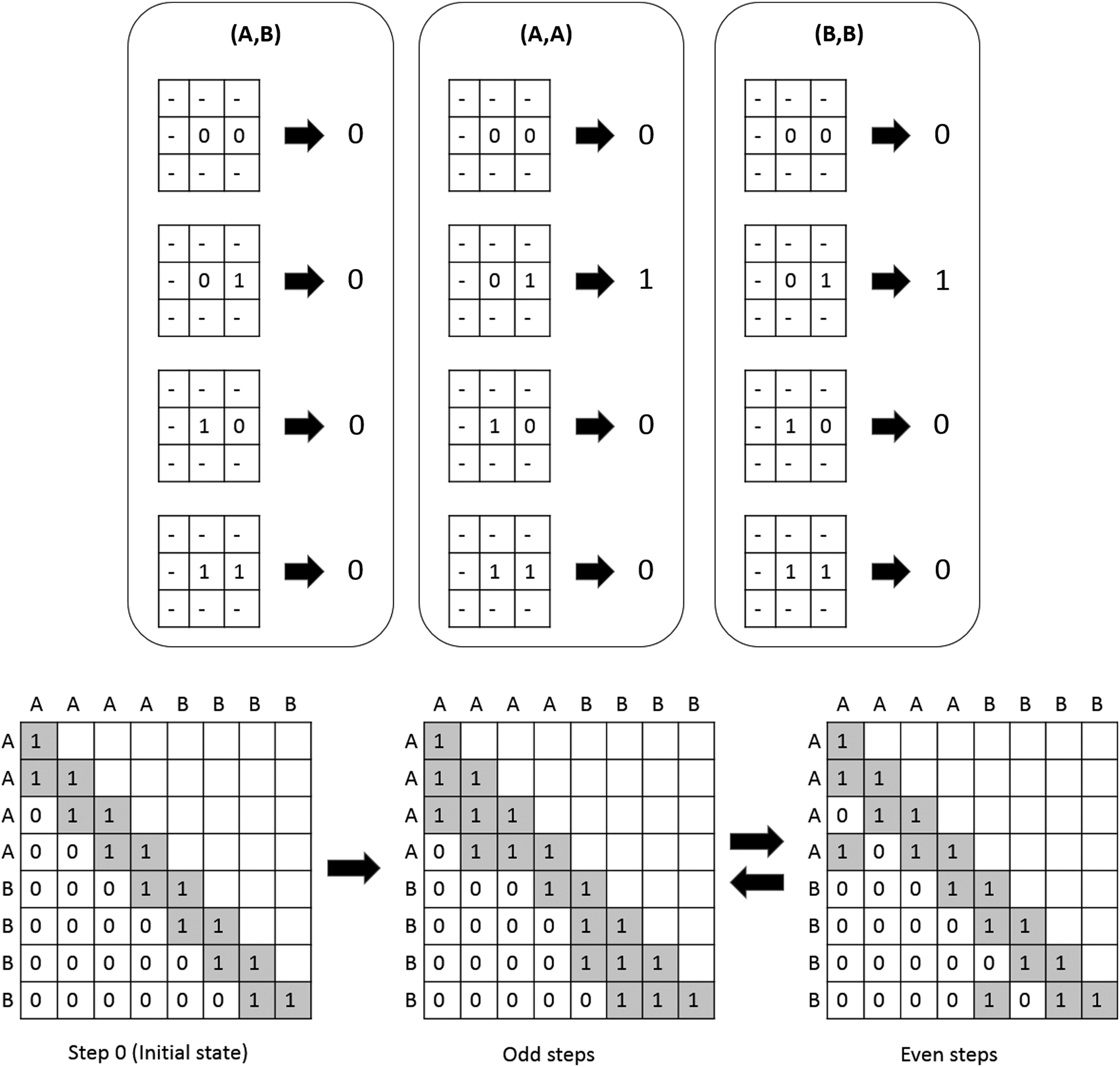
A toy model with two amino acids “A” and “B.” In here the transition function only cares about two cells in the matrix, (1,1) and (1,2), and it converges to a cycle of length 2 on the sequence “AAAABBBB.”

We can now define a transition function that takes as input a pair of amino acids \documentclass{aastex}\usepackage{amsbsy}\usepackage{amsfonts}\usepackage{amssymb}\usepackage{bm}\usepackage{mathrsfs}\usepackage{pifont}\usepackage{stmaryrd}\usepackage{textcomp}\usepackage{portland, xspace}\usepackage{amsmath, amsxtra}\usepackage{upgreek}\pagestyle{empty}\DeclareMathSizes{10}{9}{7}{6}\begin{document} $$( i , j )$$ \end{document} with the neighborhood, and output the status of the same edge \documentclass{aastex}\usepackage{amsbsy}\usepackage{amsfonts}\usepackage{amssymb}\usepackage{bm}\usepackage{mathrsfs}\usepackage{pifont}\usepackage{stmaryrd}\usepackage{textcomp}\usepackage{portland, xspace}\usepackage{amsmath, amsxtra}\usepackage{upgreek}\pagestyle{empty}\DeclareMathSizes{10}{9}{7}{6}\begin{document} $$( i , j )$$ \end{document} at the next time step. More precisely, the transition function outputs a 1 or a 0, where 1 means an edge should exist in the next time step and 0 means an edge should not exist in the next time step.

Finally, we can define an overall step function, which takes a graph as an input, and computes the transition function on each pair of vertices that does not have a permanent edge. Importantly, the original graph is left unchanged throughout this computation. The individual results of the transition functions are instead cached in a new graph, which replaces the original one at the end of the computation of the overall step function. This new graph contains all permanent edges the original graph had and has a transient edge for each pair of vertices that fulfills the following three requirements: (1) the pair does not have a permanent edge between them in the original graph; (2) the transition function outputs a one for the pair; and (3) if an edge did not exist between them in the previous graph, then the degree of neither vertices can exceed a constant we will call the interaction limit. The reasoning for the last restriction is because there is no implicit constraint in our formulation of protein folding that stops a protein from transitioning into states that are physically infeasible.

Algorithm 1 illustrates the process described above. Noticeably, we initialize the contact map on line 2 and refer to an arbitrary convergence criterion on line 13. These steps are left undefined here in this generic algorithm. However, in our experiments, we define the initial state as the matrix consisting of 0 everywhere except for the main diagonal and subdiagonal, which can be interpreted as the graph containing only permanent edges. We also use a convergence criterion that halts the process after a specified number of steps.

Algorithm 1 Protein Folding Process
1: Take an amino acid sequence S of length n as input
2: Initialize an \documentclass{aastex}\usepackage{amsbsy}\usepackage{amsfonts}\usepackage{amssymb}\usepackage{bm}\usepackage{mathrsfs}\usepackage{pifont}\usepackage{stmaryrd}\usepackage{textcomp}\usepackage{portland, xspace}\usepackage{amsmath, amsxtra}\usepackage{upgreek}\pagestyle{empty}\DeclareMathSizes{10}{9}{7}{6}\begin{document} $$n \times n$$ \end{document} matrix A to an initial state
3: loop
4: Initialize a blank \documentclass{aastex}\usepackage{amsbsy}\usepackage{amsfonts}\usepackage{amssymb}\usepackage{bm}\usepackage{mathrsfs}\usepackage{pifont}\usepackage{stmaryrd}\usepackage{textcomp}\usepackage{portland, xspace}\usepackage{amsmath, amsxtra}\usepackage{upgreek}\pagestyle{empty}\DeclareMathSizes{10}{9}{7}{6}\begin{document} $$n \times n$$ \end{document} matrix B
5: for each cell \documentclass{aastex}\usepackage{amsbsy}\usepackage{amsfonts}\usepackage{amssymb}\usepackage{bm}\usepackage{mathrsfs}\usepackage{pifont}\usepackage{stmaryrd}\usepackage{textcomp}\usepackage{portland, xspace}\usepackage{amsmath, amsxtra}\usepackage{upgreek}\pagestyle{empty}\DeclareMathSizes{10}{9}{7}{6}\begin{document} $$( i , j )$$ \end{document} in B where \documentclass{aastex}\usepackage{amsbsy}\usepackage{amsfonts}\usepackage{amssymb}\usepackage{bm}\usepackage{mathrsfs}\usepackage{pifont}\usepackage{stmaryrd}\usepackage{textcomp}\usepackage{portland, xspace}\usepackage{amsmath, amsxtra}\usepackage{upgreek}\pagestyle{empty}\DeclareMathSizes{10}{9}{7}{6}\begin{document} $$j \le i$$ \end{document} do
6: if \|i − j\|≤1 then
7: Set \documentclass{aastex}\usepackage{amsbsy}\usepackage{amsfonts}\usepackage{amssymb}\usepackage{bm}\usepackage{mathrsfs}\usepackage{pifont}\usepackage{stmaryrd}\usepackage{textcomp}\usepackage{portland, xspace}\usepackage{amsmath, amsxtra}\usepackage{upgreek}\pagestyle{empty}\DeclareMathSizes{10}{9}{7}{6}\begin{document} $${B_{i , j}}$$ \end{document} to 1, since it is a permanent edge
8: else
9: Construct a \documentclass{aastex}\usepackage{amsbsy}\usepackage{amsfonts}\usepackage{amssymb}\usepackage{bm}\usepackage{mathrsfs}\usepackage{pifont}\usepackage{stmaryrd}\usepackage{textcomp}\usepackage{portland, xspace}\usepackage{amsmath, amsxtra}\usepackage{upgreek}\pagestyle{empty}\DeclareMathSizes{10}{9}{7}{6}\begin{document} $$3 \times 3$$ \end{document} matrix U from cell \documentclass{aastex}\usepackage{amsbsy}\usepackage{amsfonts}\usepackage{amssymb}\usepackage{bm}\usepackage{mathrsfs}\usepackage{pifont}\usepackage{stmaryrd}\usepackage{textcomp}\usepackage{portland, xspace}\usepackage{amsmath, amsxtra}\usepackage{upgreek}\pagestyle{empty}\DeclareMathSizes{10}{9}{7}{6}\begin{document} $${A_{i , j}}$$ \end{document} , and the 8 cells surrounding it
10: If any cells land outside the matrix, pretend its value is 0
11: Feed U, S_i, and S_j to the transition function and set \documentclass{aastex}\usepackage{amsbsy}\usepackage{amsfonts}\usepackage{amssymb}\usepackage{bm}\usepackage{mathrsfs}\usepackage{pifont}\usepackage{stmaryrd}\usepackage{textcomp}\usepackage{portland, xspace}\usepackage{amsmath, amsxtra}\usepackage{upgreek}\pagestyle{empty}\DeclareMathSizes{10}{9}{7}{6}\begin{document} $${B_{i , j}}$$ \end{document} to its output
12: Set A to B
13: if some convergence criteria is met then
14: return A

2.2. HP-X8 models

Our description above requires parameterization of the transition function before it can be used to iterate on graphs to simulate folding dynamics. We first need to set the number of different amino acids the transition function is capable of recognizing, and what the transition function outputs for every unique set of inputs. We will refer to such parameterization of a transition function as a model.

To verify the validity of our overall approach, we need to find models that have the ability to simulate biological phenomena. Searching for such a model in the full space of possible models is obviously intractable, so instead we introduce a subset of the model space, which is both tractable and contains models that are complex enough to capture biological phenomena. First, we reduce the amino acid alphabet from 20 letters down to 2 (hydrophobic and polar), and limit the number of interactions to 8. Next, in the transition function, we will only consider two types of amino acid inputs: either both amino acids are hydrophobic or not. In particular, it means that for any matrix M, the transition function will give the same output on inputs (M,P,P and M,H,P), where H and P are the hydrophobic and polar amino acids, respectively.

Next, for the matrix input, the transition function for a pair of amino acids \documentclass{aastex}\usepackage{amsbsy}\usepackage{amsfonts}\usepackage{amssymb}\usepackage{bm}\usepackage{mathrsfs}\usepackage{pifont}\usepackage{stmaryrd}\usepackage{textcomp}\usepackage{portland, xspace}\usepackage{amsmath, amsxtra}\usepackage{upgreek}\pagestyle{empty}\DeclareMathSizes{10}{9}{7}{6}\begin{document} $$( i , j )$$ \end{document} will only consider the entries at the coordinates \documentclass{aastex}\usepackage{amsbsy}\usepackage{amsfonts}\usepackage{amssymb}\usepackage{bm}\usepackage{mathrsfs}\usepackage{pifont}\usepackage{stmaryrd}\usepackage{textcomp}\usepackage{portland, xspace}\usepackage{amsmath, amsxtra}\usepackage{upgreek}\pagestyle{empty}\DeclareMathSizes{10}{9}{7}{6}\begin{document} $$( i - 1 , j - 1 ) , ( i - 1 , i + 1 ) , ( i , j ) , ( i + 1 , i - 1 ) ,$$ \end{document} and \documentclass{aastex}\usepackage{amsbsy}\usepackage{amsfonts}\usepackage{amssymb}\usepackage{bm}\usepackage{mathrsfs}\usepackage{pifont}\usepackage{stmaryrd}\usepackage{textcomp}\usepackage{portland, xspace}\usepackage{amsmath, amsxtra}\usepackage{upgreek}\pagestyle{empty}\DeclareMathSizes{10}{9}{7}{6}\begin{document} $$( i + 1 , j + 1 )$$ \end{document} , which together form an X shape. We also consider two matrices to be equivalent if they are identical after a series of 90° rotations, which means the transition function ignores the relative linear positions of the amino acids on the chain. Under these hypotheses, our model can be defined using the 12 types of matrix inputs shown in Figure 2.

FIG. 2.

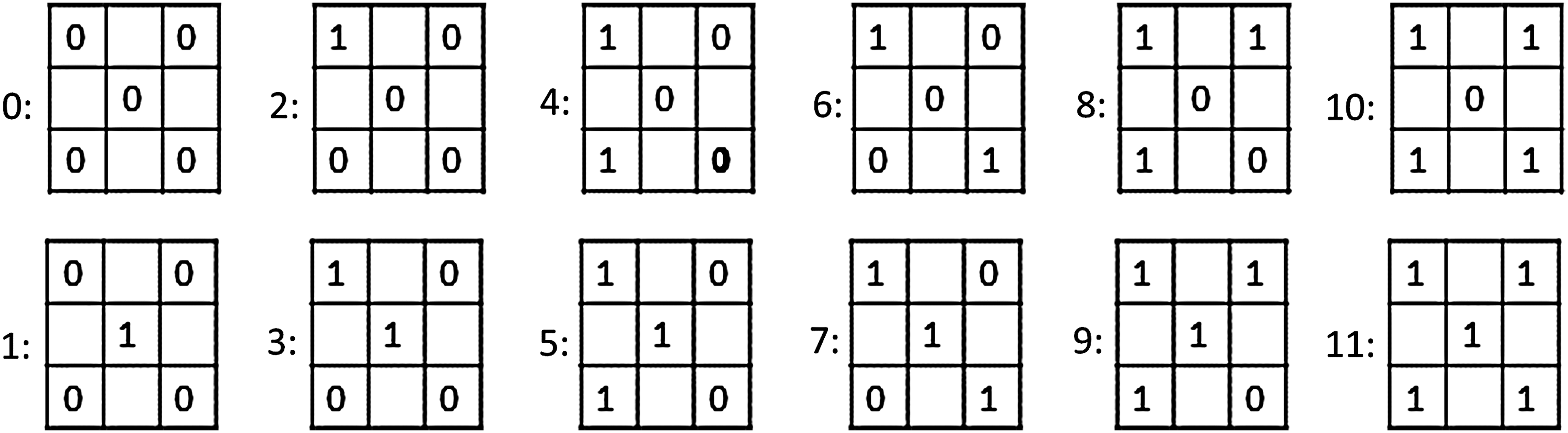
All unique input matrices of HP-X8 models.

Finally, we will say that (H,H) interactions are stronger than all other interactions. It means that if the transition function outputs 0 for a matrix and an (H,H) input, it must output 0 for any other amino acid inputs.

We call this set of models HP-X8 models. Due to these restrictions, there are only a total of 531441 models with different parameters. This reduction in complexity allows brute force enumeration and testing of these models; however, there is a significant sacrifice in the amount of information that is lost. Although it is unlikely for HP-X8 models to be able to make detailed predictions of protein dynamics, we find that some of these models do capture interesting phenomena, and their ability to do so despite the loss of information is indicative of the expressivity and biological relevance that our overall approach has.

3. Results and Discussion

3.1. Brute force enumeration

We tested all HP-X8 models on random sequences, and we considered those that did not halt within five time steps to be viable, since heuristically speaking five time steps would not be enough to generate interesting structures. For our experiments, we always assumed that folding starts with no transient edges. This filtering process left us with 55404 viable models.

To test the viable models, we extracted a diverse set of 95 proteins from the BetaSheet916 data set (Cheng and Baldi, 2005), with sizes ranging from 41 to 120 residues, for which the native 3D structures are available with a resolution better than 2.5Å. The extracted proteins belong to all of the main protein families (such as \documentclass{aastex}\usepackage{amsbsy}\usepackage{amsfonts}\usepackage{amssymb}\usepackage{bm}\usepackage{mathrsfs}\usepackage{pifont}\usepackage{stmaryrd}\usepackage{textcomp}\usepackage{portland, xspace}\usepackage{amsmath, amsxtra}\usepackage{upgreek}\pagestyle{empty}\DeclareMathSizes{10}{9}{7}{6}\begin{document} $$\alpha / \beta$$ \end{document} , \documentclass{aastex}\usepackage{amsbsy}\usepackage{amsfonts}\usepackage{amssymb}\usepackage{bm}\usepackage{mathrsfs}\usepackage{pifont}\usepackage{stmaryrd}\usepackage{textcomp}\usepackage{portland, xspace}\usepackage{amsmath, amsxtra}\usepackage{upgreek}\pagestyle{empty}\DeclareMathSizes{10}{9}{7}{6}\begin{document} $$\alpha + \beta$$ \end{document} , and all- \documentclass{aastex}\usepackage{amsbsy}\usepackage{amsfonts}\usepackage{amssymb}\usepackage{bm}\usepackage{mathrsfs}\usepackage{pifont}\usepackage{stmaryrd}\usepackage{textcomp}\usepackage{portland, xspace}\usepackage{amsmath, amsxtra}\usepackage{upgreek}\pagestyle{empty}\DeclareMathSizes{10}{9}{7}{6}\begin{document} $$\beta$$ \end{document} ) as defined by structural classification of proteins (SCOP). The sequence identity between any pair of sequences in the data set is between 15% and 20%, and only proteins containing less than six strands were extracted. BetaSheet916 is a benchmark that has been a routinely adopted set for \documentclass{aastex}\usepackage{amsbsy}\usepackage{amsfonts}\usepackage{amssymb}\usepackage{bm}\usepackage{mathrsfs}\usepackage{pifont}\usepackage{stmaryrd}\usepackage{textcomp}\usepackage{portland, xspace}\usepackage{amsmath, amsxtra}\usepackage{upgreek}\pagestyle{empty}\DeclareMathSizes{10}{9}{7}{6}\begin{document} $$\beta$$ \end{document} -residue pairs, \documentclass{aastex}\usepackage{amsbsy}\usepackage{amsfonts}\usepackage{amssymb}\usepackage{bm}\usepackage{mathrsfs}\usepackage{pifont}\usepackage{stmaryrd}\usepackage{textcomp}\usepackage{portland, xspace}\usepackage{amsmath, amsxtra}\usepackage{upgreek}\pagestyle{empty}\DeclareMathSizes{10}{9}{7}{6}\begin{document} $$\beta$$ \end{document} -strand pairs, and \documentclass{aastex}\usepackage{amsbsy}\usepackage{amsfonts}\usepackage{amssymb}\usepackage{bm}\usepackage{mathrsfs}\usepackage{pifont}\usepackage{stmaryrd}\usepackage{textcomp}\usepackage{portland, xspace}\usepackage{amsmath, amsxtra}\usepackage{upgreek}\pagestyle{empty}\DeclareMathSizes{10}{9}{7}{6}\begin{document} $$\beta$$ \end{document} -sheet prediction methods. In addition, the proteins in BetaSheet916 have played a central role in protein folding studies by being the system of choice in a vast body of experimental and theoretical studies. The table for reduction of the 20 amino acids to the HP alphabet is provided in Figure 3.

FIG. 3.

Translation table for the 20 amino acid alphabet to the HP alphabet. HP, hydrophobic/polar.

For each protein, we ran each model for 100 time steps and computed the harmonic mean of the precision and recall (F1 Score). For the purposes of scoring how well a model performs, we define an interaction as existing if a pair of amino acids are closer than 10 nm apart, and we say we have a true positive if a predicted interaction lies within two amino acids of the real contact, since those parameters appear to produce the best results. Due to the abundance of short range contacts, models that generate large amounts of those indiscriminately usually end up with the best F1 score. However, it does appear to be a decent heuristic, as some models that do score reasonable well do display interesting features. Therefore, we took the 50 models that scored best with the F1 score and ran each model for 200 time steps, this time applying a complementary scoring function: \documentclass{aastex}\usepackage{amsbsy}\usepackage{amsfonts}\usepackage{amssymb}\usepackage{bm}\usepackage{mathrsfs}\usepackage{pifont}\usepackage{stmaryrd}\usepackage{textcomp}\usepackage{portland, xspace}\usepackage{amsmath, amsxtra}\usepackage{upgreek}\pagestyle{empty}\DeclareMathSizes{10}{9}{7}{6}\begin{document} \begin{align*} {F_1} \times ( \mathop \sum \limits_{d \in 5 , 6 , 7 \ldots} \sqrt {{c_d} \sqrt {d - 4} } + \sqrt {{c_4}} + \sqrt {{c_3}} ) , \tag{1} \end{align*} \end{document}

where c_d is the number of contacts detected that are d amino acids apart, and F₁ is the F1 score. This function takes into account that it is better to have a diverse range of contacts at all distances by using a sum of concave functions and includes a range dependent factors so that long-range contacts are more heavily favored than close-range ones. We also performed the whole process for a control set, which consisted of the same proteins, but we shuffled the sequence of the amino acids before starting the process. Figure 4 contains some examples of the resulting contact maps, and a comparison to the controls (a comprehensive list of the results can be found in the Supplementary Material).

FIG. 4.

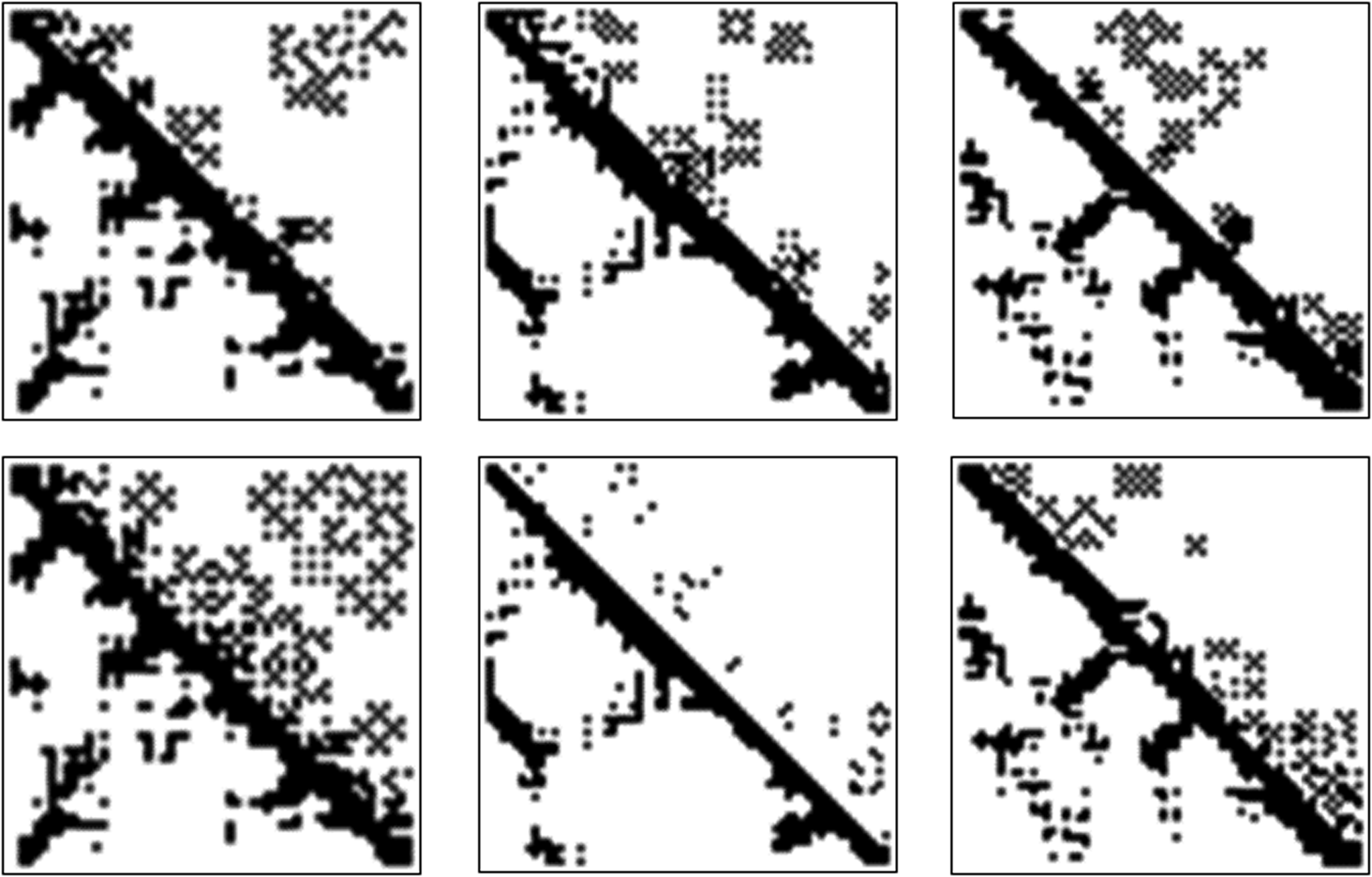
On the top row are optimal HP-X8 models iterated on 1B13, 1SOY, and 1NR2 for 190, 197, and 155 time steps, respectively, from left to right. Below them are the results of the same experiment on the same proteins, where the sequence was randomized. The lower triangle is the contact map extracted from the protein data bank (PDB), while the upper triangle is the output of the model.

Figure 4 illustrates an interesting observation. We discover that for many sequences there exists an HP-X8 model that takes a protein from a state with no transient edges to one whose adjacency matrix reasonably resembles the real protein contact map. These results support our hypothesis by showing that local perturbations in topology are indeed capable of generating protein folds that look realistic. By comparing our results to our controls, we observe that without sequence information, HP-X8 models are less capable of carrying a protein into a state that resembles the real protein contact map, which rules out the possibility that our results are a consequence of the robustness of the HP-X8 models. We have included the data pertaining to this comparison in the Supplementary Material.

3.2. Consensus model

In the previous section, we have provided evidence that our approach has merit. Nonetheless, if our models are reflective of reality, it is reasonable to suspect that all the models we have captured in the last experiment are noisy approximations of a single model. Therefore, we would like to assess the degree to which the models we have captured approximate reality. To this end we measure the agreements between the transition functions of the captured models.

We allow each protein to place a vote for what should happen for each input for the transition function, and we have recorded the results of the vote in Figure 5a. Under the null hypothesis that each protein selects its best model uniformly at random, we observe statistically significant (p-value under 0.05) agreement for all inputs except 3.

FIG. 5.

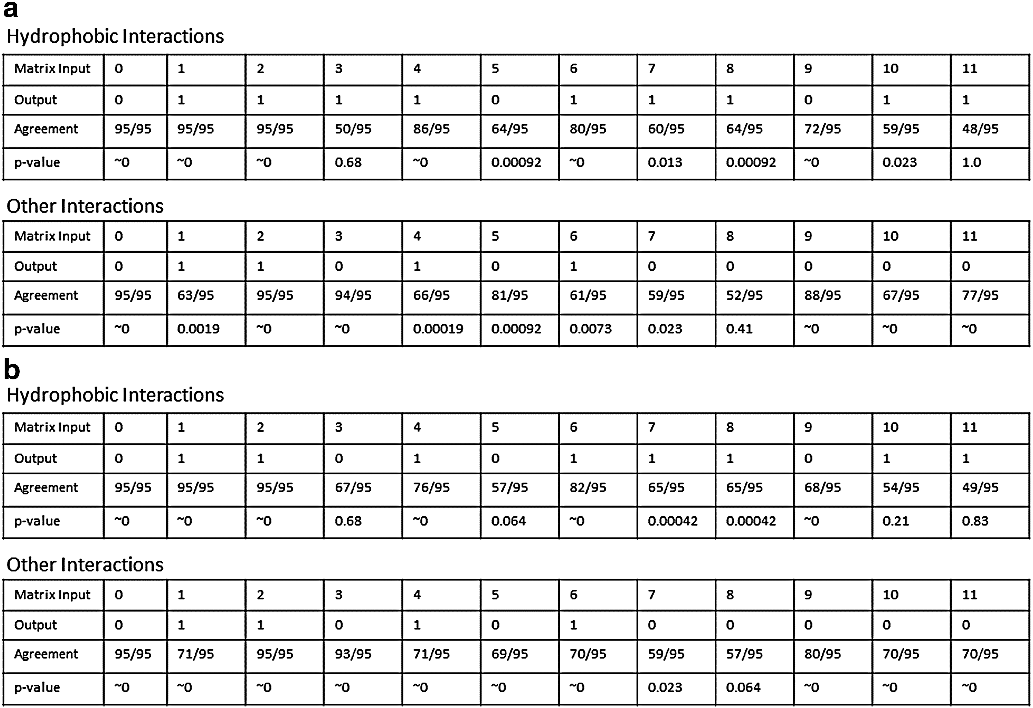
Consensus results. (a) The agreements between the best models of each protein. (b) The agreements between the best models of each protein for the control experiment.

Similarly, we also checked model agreement for our control set in the same way. Figure 5b shows our results. The overall agreement levels seem to be approximately the same as our result set.

Unsurprisingly, these results suggest that the HP-X8 models are far too simplistic to fully capture a general underlying model. This is quite plausible, since models based on the HP alphabet lose a large amount of information when transitioning from a 20-letter alphabet to a 2-letter alphabet. Despite this, it is clear that our framework captures a signal, since there are statistically significant agreements in most of the rules. We hypothesize that we are capturing the necessary rules that are required for a transition function to generate biological structures. Our control experiment supports this notion, since the aggregate function from the control experiment is very similar to the aggregate function from our main experiment with similar levels of agreement.

3.3. Stable states

We are now presenting the main theoretical results of this study. Importantly, in the remainder of this article, we will consider the full generalized models instead of the subset of HP-X8 models we have previously used to demonstrate the biological relevance of this system.

Our study aims to characterize the difficulty for a sequence to have a stable conformation (i.e., state) in this framework. Interestingly, our models enable us to naturally define the concept of a stable state. Let a state s_t be a graph (or its adjacency matrix) representing a protein structure at a given time step t. Using our models, a state gives all the information required to compute the next state \documentclass{aastex}\usepackage{amsbsy}\usepackage{amsfonts}\usepackage{amssymb}\usepackage{bm}\usepackage{mathrsfs}\usepackage{pifont}\usepackage{stmaryrd}\usepackage{textcomp}\usepackage{portland, xspace}\usepackage{amsmath, amsxtra}\usepackage{upgreek}\pagestyle{empty}\DeclareMathSizes{10}{9}{7}{6}\begin{document} $$t + 1$$ \end{document} . Thus, we can decide if a folding is complete if the next state \documentclass{aastex}\usepackage{amsbsy}\usepackage{amsfonts}\usepackage{amssymb}\usepackage{bm}\usepackage{mathrsfs}\usepackage{pifont}\usepackage{stmaryrd}\usepackage{textcomp}\usepackage{portland, xspace}\usepackage{amsmath, amsxtra}\usepackage{upgreek}\pagestyle{empty}\DeclareMathSizes{10}{9}{7}{6}\begin{document} $${s_{t + 1}}$$ \end{document} given by the step function is identical to the current state s_t. The state s_t is called a stable state (or stable structure).

Intuitively, the stability of a state is dependent on the sequence. This observation leads naturally to several interesting questions such as given a transition function, are there certain states that are inherently unstable, and if yes, is it possible to find them? Such questions are closely related to the problem of protein design, since if a state is inherently unstable it becomes also undesignable.

To answer these questions, let us consider a problem that we will call the stable state characterization problem.

Definition 1. Given a graph with n vertices representing a state and a set of k amino acids along with a transition function, determine if there exists a sequence of n amino acids taken from the set such that the state is a stable state.

Theorem 1. Stable state characterization is \documentclass{aastex}\usepackage{amsbsy}\usepackage{amsfonts}\usepackage{amssymb}\usepackage{bm}\usepackage{mathrsfs}\usepackage{pifont}\usepackage{stmaryrd}\usepackage{textcomp}\usepackage{portland, xspace}\usepackage{amsmath, amsxtra}\usepackage{upgreek}\pagestyle{empty}\DeclareMathSizes{10}{9}{7}{6}\begin{document} $${ \cal N}{ \cal P}$$ \end{document} -hard.

Proof. Stable state characterization is polynomially reducible from vertex coloring, which is a classical \documentclass{aastex}\usepackage{amsbsy}\usepackage{amsfonts}\usepackage{amssymb}\usepackage{bm}\usepackage{mathrsfs}\usepackage{pifont}\usepackage{stmaryrd}\usepackage{textcomp}\usepackage{portland, xspace}\usepackage{amsmath, amsxtra}\usepackage{upgreek}\pagestyle{empty}\DeclareMathSizes{10}{9}{7}{6}\begin{document} $${ \cal N}{ \cal P}$$ \end{document} -complete problem.

It suffices to introduce amino acids that correspond to colors and make edges unstable when two amino acids representing the same color interact with each other, and make edges stable when the amino acids are different. As a construction detail, we make sure that edges do not spontaneously form. A string of amino acids that stabilize the state must then encode a graph coloring. Note that the interaction limit does not come into play here, since that only restricts the formation of new edges and not whether an edge could break.

As a construction detail, we need to interlace the original graph with noninteracting amino acids. We can take the adjacency matrix representing the original problem and interlace blank rows and columns between each row and column of the original adjacency matrix. The reason this is required is because adjacent amino acids are connected by default, which would limit the graph topologies that could be encoded if we do not interlace.

If a sequence that stabilizes the state exists, then we can read the coloring of the parts of the sequence that correspond to the original matrix. The coloring would be valid, since otherwise one of the edges would be unstable. Conversely, if a valid coloring exists, then we can make a sequence of amino acids corresponding to that coloring and interlace that sequence with any amino acid, since the corresponding rows and columns are blank and therefore stable. This will provide a sequence that would stabilize the new adjacency matrix, since the rows and columns in the original adjacency matrix would be stabilized by the coloring by our construction.

Thus, a solution to the stable state characterization problem exists if and only if a solution to the original vertex coloring problem exists. If the original graph was also represented as an adjacency matrix, then the new matrix can be created in linear time. Thus, there is a polynomial reduction from vertex coloring to stable state characterization, and therefore, stable state characterization is \documentclass{aastex}\usepackage{amsbsy}\usepackage{amsfonts}\usepackage{amssymb}\usepackage{bm}\usepackage{mathrsfs}\usepackage{pifont}\usepackage{stmaryrd}\usepackage{textcomp}\usepackage{portland, xspace}\usepackage{amsmath, amsxtra}\usepackage{upgreek}\pagestyle{empty}\DeclareMathSizes{10}{9}{7}{6}\begin{document} $${ \cal N}{ \cal P}$$ \end{document} -hard. ■

Corollary 1. Stable state characterization is \documentclass{aastex}\usepackage{amsbsy}\usepackage{amsfonts}\usepackage{amssymb}\usepackage{bm}\usepackage{mathrsfs}\usepackage{pifont}\usepackage{stmaryrd}\usepackage{textcomp}\usepackage{portland, xspace}\usepackage{amsmath, amsxtra}\usepackage{upgreek}\pagestyle{empty}\DeclareMathSizes{10}{9}{7}{6}\begin{document} $${ \cal N}{ \cal P}$$ \end{document} -complete.

Proof. This follows immediately from the above theorem, since a sequence of amino acids that allow the state to be stable would be a suitable certificate. The evaluation given such a sequence takes time \documentclass{aastex}\usepackage{amsbsy}\usepackage{amsfonts}\usepackage{amssymb}\usepackage{bm}\usepackage{mathrsfs}\usepackage{pifont}\usepackage{stmaryrd}\usepackage{textcomp}\usepackage{portland, xspace}\usepackage{amsmath, amsxtra}\usepackage{upgreek}\pagestyle{empty}\DeclareMathSizes{10}{9}{7}{6}\begin{document} $${ \cal O} ( {n^2} )$$ \end{document} , where n is the length of the sequence. ■

Thus, in the general setting it is impossible to provide an efficient method of deciding whether a particular structure can be stable or not, unless \documentclass{aastex}\usepackage{amsbsy}\usepackage{amsfonts}\usepackage{amssymb}\usepackage{bm}\usepackage{mathrsfs}\usepackage{pifont}\usepackage{stmaryrd}\usepackage{textcomp}\usepackage{portland, xspace}\usepackage{amsmath, amsxtra}\usepackage{upgreek}\pagestyle{empty}\DeclareMathSizes{10}{9}{7}{6}\begin{document} $${ \cal P} = { \cal N}{ \cal P}$$ \end{document} . Remarkably, we note that this also proves that there can be states that are inherently unstable.

Since a vertex coloring problem can encode 3-SAT at three colors, stable state characterization can be \documentclass{aastex}\usepackage{amsbsy}\usepackage{amsfonts}\usepackage{amssymb}\usepackage{bm}\usepackage{mathrsfs}\usepackage{pifont}\usepackage{stmaryrd}\usepackage{textcomp}\usepackage{portland, xspace}\usepackage{amsmath, amsxtra}\usepackage{upgreek}\pagestyle{empty}\DeclareMathSizes{10}{9}{7}{6}\begin{document} $${ \cal N}{ \cal P}$$ \end{document} -complete if the transition function uses three amino acids or more. However, perhaps the problem only becomes NP-complete when the states are unrealistic, for instance, when a single amino acid has an unrealistic amount of interactions. The following theorem shows that that is not the case.

Theorem 2. Vertex coloring with k colors where the maximum degree is \documentclass{aastex}\usepackage{amsbsy}\usepackage{amsfonts}\usepackage{amssymb}\usepackage{bm}\usepackage{mathrsfs}\usepackage{pifont}\usepackage{stmaryrd}\usepackage{textcomp}\usepackage{portland, xspace}\usepackage{amsmath, amsxtra}\usepackage{upgreek}\pagestyle{empty}\DeclareMathSizes{10}{9}{7}{6}\begin{document} $$2k - 1$$ \end{document} is NP-complete, given that \documentclass{aastex}\usepackage{amsbsy}\usepackage{amsfonts}\usepackage{amssymb}\usepackage{bm}\usepackage{mathrsfs}\usepackage{pifont}\usepackage{stmaryrd}\usepackage{textcomp}\usepackage{portland, xspace}\usepackage{amsmath, amsxtra}\usepackage{upgreek}\pagestyle{empty}\DeclareMathSizes{10}{9}{7}{6}\begin{document} $$k > 2$$ \end{document} .

Proof. We can reduce this problem from arbitrary k-coloring. Note that if a vertex has more than \documentclass{aastex}\usepackage{amsbsy}\usepackage{amsfonts}\usepackage{amssymb}\usepackage{bm}\usepackage{mathrsfs}\usepackage{pifont}\usepackage{stmaryrd}\usepackage{textcomp}\usepackage{portland, xspace}\usepackage{amsmath, amsxtra}\usepackage{upgreek}\pagestyle{empty}\DeclareMathSizes{10}{9}{7}{6}\begin{document} $$2k - 1$$ \end{document} incoming edges, we can construct a device, where two unconnected nodes are connected to the same \documentclass{aastex}\usepackage{amsbsy}\usepackage{amsfonts}\usepackage{amssymb}\usepackage{bm}\usepackage{mathrsfs}\usepackage{pifont}\usepackage{stmaryrd}\usepackage{textcomp}\usepackage{portland, xspace}\usepackage{amsmath, amsxtra}\usepackage{upgreek}\pagestyle{empty}\DeclareMathSizes{10}{9}{7}{6}\begin{document} $$k - 1$$ \end{document} other nodes. This would then require the two nodes to be the same color. We can keep doing this to create a chain, where each link must be the same color. This way, each link only requires one more incoming edge, thus the maximum degree of this graph is \documentclass{aastex}\usepackage{amsbsy}\usepackage{amsfonts}\usepackage{amssymb}\usepackage{bm}\usepackage{mathrsfs}\usepackage{pifont}\usepackage{stmaryrd}\usepackage{textcomp}\usepackage{portland, xspace}\usepackage{amsmath, amsxtra}\usepackage{upgreek}\pagestyle{empty}\DeclareMathSizes{10}{9}{7}{6}\begin{document} $$2 ( k - 1 ) + 1 = 2k - 1$$ \end{document} . Since each node originally can have at most as many incoming edges as there are nodes, this modification represents at most a polynomial increase in the number of nodes, thus the reduction is polynomial. ■

From the way our proof of \documentclass{aastex}\usepackage{amsbsy}\usepackage{amsfonts}\usepackage{amssymb}\usepackage{bm}\usepackage{mathrsfs}\usepackage{pifont}\usepackage{stmaryrd}\usepackage{textcomp}\usepackage{portland, xspace}\usepackage{amsmath, amsxtra}\usepackage{upgreek}\pagestyle{empty}\DeclareMathSizes{10}{9}{7}{6}\begin{document} $${ \cal N}{ \cal P}$$ \end{document} -completeness is constructed, it follows from the theorem that realistic instances of the stable state characterization problem do not necessarily simplify the problem.

3.4. Implications for the inverse folding problem

The results presented in the last section have implications for the inverse folding problem, where given a structure, one has to produce a sequence that can stabilize the structure. If the inverse folding problem can be solved efficiently, then we can create an oracle algorithm to solve stable state characterization efficiently, where we run inverse folding on our sequence, and output whether a sequence was found or not. Thus, it follows that there exists no efficient algorithm for inverse folding, unless \documentclass{aastex}\usepackage{amsbsy}\usepackage{amsfonts}\usepackage{amssymb}\usepackage{bm}\usepackage{mathrsfs}\usepackage{pifont}\usepackage{stmaryrd}\usepackage{textcomp}\usepackage{portland, xspace}\usepackage{amsmath, amsxtra}\usepackage{upgreek}\pagestyle{empty}\DeclareMathSizes{10}{9}{7}{6}\begin{document} $${ \cal P} = { \cal N}{ \cal P}$$ \end{document} .

However, this conclusion must be completed. In our model, it is possible that a stable conformation for a protein is represented by a small cycle of states rather than by a single stable state. Intuitively, the length of a cycle roughly corresponds to stability, with shorter cycles being more stable. We can therefore define an optimization problem analogous to the stable state characterization problem, where given the same inputs, one is asked to provide a sequence such that the provided structure, while not necessarily stable, does eventually return after a number of steps, and such that the number of steps required before the structure returns is minimized. This is also \documentclass{aastex}\usepackage{amsbsy}\usepackage{amsfonts}\usepackage{amssymb}\usepackage{bm}\usepackage{mathrsfs}\usepackage{pifont}\usepackage{stmaryrd}\usepackage{textcomp}\usepackage{portland, xspace}\usepackage{amsmath, amsxtra}\usepackage{upgreek}\pagestyle{empty}\DeclareMathSizes{10}{9}{7}{6}\begin{document} $${ \cal N}{ \cal P}$$ \end{document} -hard, since if the optimal cycle contains only one state, a correct optimization algorithm will find a sequence that allows this, and will in turn solve the stable state characterization problem.

In our reduction of the stable state characterization problem, we showed that for a specific model with fixed parameters, the inverse folding problem is \documentclass{aastex}\usepackage{amsbsy}\usepackage{amsfonts}\usepackage{amssymb}\usepackage{bm}\usepackage{mathrsfs}\usepackage{pifont}\usepackage{stmaryrd}\usepackage{textcomp}\usepackage{portland, xspace}\usepackage{amsmath, amsxtra}\usepackage{upgreek}\pagestyle{empty}\DeclareMathSizes{10}{9}{7}{6}\begin{document} $${ \cal N}{ \cal P}$$ \end{document} -complete. To our knowledge, this is the first time evidence has been presented that shows the difficulty of the inverse folding problem scales with the size of the length of the protein, as opposed to the size of the parameters of the model in off-lattice models.

3.5. Complexity of stable state characterization with two amino acids

Our proof above shows that stable state characterization becomes \documentclass{aastex}\usepackage{amsbsy}\usepackage{amsfonts}\usepackage{amssymb}\usepackage{bm}\usepackage{mathrsfs}\usepackage{pifont}\usepackage{stmaryrd}\usepackage{textcomp}\usepackage{portland, xspace}\usepackage{amsmath, amsxtra}\usepackage{upgreek}\pagestyle{empty}\DeclareMathSizes{10}{9}{7}{6}\begin{document} $${ \cal N}{ \cal P}$$ \end{document} -complete at three amino acids. We will now show that for any transition function that only recognizes two amino acids, the problem lies in \documentclass{aastex}\usepackage{amsbsy}\usepackage{amsfonts}\usepackage{amssymb}\usepackage{bm}\usepackage{mathrsfs}\usepackage{pifont}\usepackage{stmaryrd}\usepackage{textcomp}\usepackage{portland, xspace}\usepackage{amsmath, amsxtra}\usepackage{upgreek}\pagestyle{empty}\DeclareMathSizes{10}{9}{7}{6}\begin{document} $${ \cal P}$$ \end{document} . In particular, this shows that for the HP-X8 models, stable state characterization can be done efficiently, and therefore, the inverse folding problem can also be solved efficiently.

Theorem 3. Stable state characterization with two unique amino acids is in \documentclass{aastex}\usepackage{amsbsy}\usepackage{amsfonts}\usepackage{amssymb}\usepackage{bm}\usepackage{mathrsfs}\usepackage{pifont}\usepackage{stmaryrd}\usepackage{textcomp}\usepackage{portland, xspace}\usepackage{amsmath, amsxtra}\usepackage{upgreek}\pagestyle{empty}\DeclareMathSizes{10}{9}{7}{6}\begin{document} $${ \cal P}$$ \end{document} .

Proof. For simplicity, we will show this by reducing the problem to 2-SAT, which can be solved in polynomial time, instead of providing an actual algorithm.

Let us call the two amino acids T and F. We will also assign each amino acid a Boolean value, such that T is true and F is false. Let S be a sequence consisting of T and F, and let A be the adjacency matrix representing the state we want to stabilize. Each cell, based on its surroundings, can be constrained in a way that can be expressed as a 2-CNF, where a and b are the interacting amino acids.

The cell is stable only if the interaction is between T and T	\documentclass{aastex}\usepackage{amsbsy}\usepackage{amsfonts}\usepackage{amssymb}\usepackage{bm}\usepackage{mathrsfs}\usepackage{pifont}\usepackage{stmaryrd}\usepackage{textcomp}\usepackage{portland, xspace}\usepackage{amsmath, amsxtra}\usepackage{upgreek}\pagestyle{empty}\DeclareMathSizes{10}{9}{7}{6}\begin{document} $$( a \vee a ) \wedge ( b \vee b )$$ \end{document}
The cell is stable only if the interaction is between F and F	\documentclass{aastex}\usepackage{amsbsy}\usepackage{amsfonts}\usepackage{amssymb}\usepackage{bm}\usepackage{mathrsfs}\usepackage{pifont}\usepackage{stmaryrd}\usepackage{textcomp}\usepackage{portland, xspace}\usepackage{amsmath, amsxtra}\usepackage{upgreek}\pagestyle{empty}\DeclareMathSizes{10}{9}{7}{6}\begin{document} $$( \neg a \vee \neg a ) \wedge ( \neg b \vee \neg b )$$ \end{document}
The cell is stable only if the interaction is between T and F	\documentclass{aastex}\usepackage{amsbsy}\usepackage{amsfonts}\usepackage{amssymb}\usepackage{bm}\usepackage{mathrsfs}\usepackage{pifont}\usepackage{stmaryrd}\usepackage{textcomp}\usepackage{portland, xspace}\usepackage{amsmath, amsxtra}\usepackage{upgreek}\pagestyle{empty}\DeclareMathSizes{10}{9}{7}{6}\begin{document} $$( a \vee b ) \wedge ( \neg a \vee \neg b )$$ \end{document}
The cell is unstable only if the interaction is between T and T	\documentclass{aastex}\usepackage{amsbsy}\usepackage{amsfonts}\usepackage{amssymb}\usepackage{bm}\usepackage{mathrsfs}\usepackage{pifont}\usepackage{stmaryrd}\usepackage{textcomp}\usepackage{portland, xspace}\usepackage{amsmath, amsxtra}\usepackage{upgreek}\pagestyle{empty}\DeclareMathSizes{10}{9}{7}{6}\begin{document} $$( \neg a \vee \neg b )$$ \end{document}
The cell is unstable only if the interaction is between F and F	\documentclass{aastex}\usepackage{amsbsy}\usepackage{amsfonts}\usepackage{amssymb}\usepackage{bm}\usepackage{mathrsfs}\usepackage{pifont}\usepackage{stmaryrd}\usepackage{textcomp}\usepackage{portland, xspace}\usepackage{amsmath, amsxtra}\usepackage{upgreek}\pagestyle{empty}\DeclareMathSizes{10}{9}{7}{6}\begin{document} $$( a \vee b )$$ \end{document}
The cell is unstable only if the interaction is between T and F	\documentclass{aastex}\usepackage{amsbsy}\usepackage{amsfonts}\usepackage{amssymb}\usepackage{bm}\usepackage{mathrsfs}\usepackage{pifont}\usepackage{stmaryrd}\usepackage{textcomp}\usepackage{portland, xspace}\usepackage{amsmath, amsxtra}\usepackage{upgreek}\pagestyle{empty}\DeclareMathSizes{10}{9}{7}{6}\begin{document} $$( a \vee \neg b ) \wedge ( \neg a \vee b )$$ \end{document}
The cell is always stable	\documentclass{aastex}\usepackage{amsbsy}\usepackage{amsfonts}\usepackage{amssymb}\usepackage{bm}\usepackage{mathrsfs}\usepackage{pifont}\usepackage{stmaryrd}\usepackage{textcomp}\usepackage{portland, xspace}\usepackage{amsmath, amsxtra}\usepackage{upgreek}\pagestyle{empty}\DeclareMathSizes{10}{9}{7}{6}\begin{document} $$( a \vee \neg a )$$ \end{document}
The cell is always unstable	\documentclass{aastex}\usepackage{amsbsy}\usepackage{amsfonts}\usepackage{amssymb}\usepackage{bm}\usepackage{mathrsfs}\usepackage{pifont}\usepackage{stmaryrd}\usepackage{textcomp}\usepackage{portland, xspace}\usepackage{amsmath, amsxtra}\usepackage{upgreek}\pagestyle{empty}\DeclareMathSizes{10}{9}{7}{6}\begin{document} $$( a \vee a ) \wedge ( \neg a \vee \neg a )$$ \end{document}

We join all this with conjunctions to produce the 2-CNF, which can be satisfied if and only if there exists a sequence of T and F that stabilize the state. This reduction produces a 2-CNF that is no larger than a constant factor of the size of the adjacency matrix. Thus, this reduction can be done in polynomial time, and since 2-SAT can be solved in polynomial time, this problem can be solved in polynomial time.

Therefore, stable state characterization with two unique amino acids is in \documentclass{aastex}\usepackage{amsbsy}\usepackage{amsfonts}\usepackage{amssymb}\usepackage{bm}\usepackage{mathrsfs}\usepackage{pifont}\usepackage{stmaryrd}\usepackage{textcomp}\usepackage{portland, xspace}\usepackage{amsmath, amsxtra}\usepackage{upgreek}\pagestyle{empty}\DeclareMathSizes{10}{9}{7}{6}\begin{document} $${ \cal P}$$ \end{document} . ■

3.6. Expressivity of transition functions

It is easy to solve stable state characterization if we restrict the number of amino acids we use to 2. So is there any reason to use any more? The following result shows that systems with more amino acids are more expressive in terms of the stable states that it can allow, implying that there is value in having a system that recognizes more amino acids.

Theorem 4. Suppose we are given an adjacency matrix which requires n unique amino acids to ensure its stability. Then supposing that no interaction of an amino acid with itself is completely stable, we can construct an adjacency matrix which must require k amino acids to stabilize, where \documentclass{aastex}\usepackage{amsbsy}\usepackage{amsfonts}\usepackage{amssymb}\usepackage{bm}\usepackage{mathrsfs}\usepackage{pifont}\usepackage{stmaryrd}\usepackage{textcomp}\usepackage{portland, xspace}\usepackage{amsmath, amsxtra}\usepackage{upgreek}\pagestyle{empty}\DeclareMathSizes{10}{9}{7}{6}\begin{document} $$k > n$$ \end{document} .

Proof. We construct a new adjacency matrix, where we start off by taking the original adjacency matrix and adding an extra row to the top and bottom, and an extra column to the left and right. We then take this matrix and copy it diagonally n times.

If this results in an adjacency matrix that requires \documentclass{aastex}\usepackage{amsbsy}\usepackage{amsfonts}\usepackage{amssymb}\usepackage{bm}\usepackage{mathrsfs}\usepackage{pifont}\usepackage{stmaryrd}\usepackage{textcomp}\usepackage{portland, xspace}\usepackage{amsmath, amsxtra}\usepackage{upgreek}\pagestyle{empty}\DeclareMathSizes{10}{9}{7}{6}\begin{document} $$n + 1$$ \end{document} unique amino acids to ensure stability, we are done. Otherwise, we required at least n unique amino acids to ensure stability of this new adjacency matrix, since each submatrix that resembles the original matrix requires at least n unique amino acids to ensure stability. Furthermore, in any stabilizing sequence, it is possible to pick a set of n amino acids such that they are all distinct, and there are at least two amino acids between any two selected, since each submatrix requires all n amino acids to stabilize.

Let S be the set of \documentclass{aastex}\usepackage{amsbsy}\usepackage{amsfonts}\usepackage{amssymb}\usepackage{bm}\usepackage{mathrsfs}\usepackage{pifont}\usepackage{stmaryrd}\usepackage{textcomp}\usepackage{portland, xspace}\usepackage{amsmath, amsxtra}\usepackage{upgreek}\pagestyle{empty}\DeclareMathSizes{10}{9}{7}{6}\begin{document} $$( sequence \times transitionfunction )$$ \end{document} tuples that ensure stability of the matrix with only n unique amino acids in the sequence. Assume that each transition function makes use of at most n amino acids. This is inconsequential, since if only n unique amino acids are used, then any transition function using a larger set of amino acids can be truncated to only those used. Therefore, S is clearly finite.

For each element s present in S, add three rows to the bottom of the adjacency matrix. Then pick out n unique amino acids in the sequence such that no two amino acids are spaced closer than two amino acids apart. For each amino acid, find the cell at which that amino acid interacts with the one on the second row that was added and then arrange that cell such that if the identity of the new amino acid was itself, it would be unstable according to the transition function. This is always possible by our assumption.

Once we have finished doing this, it ensures that for that particular sequence and transition function, there exists no amino acid that stabilizes that contact matrix. If we do it for all \documentclass{aastex}\usepackage{amsbsy}\usepackage{amsfonts}\usepackage{amssymb}\usepackage{bm}\usepackage{mathrsfs}\usepackage{pifont}\usepackage{stmaryrd}\usepackage{textcomp}\usepackage{portland, xspace}\usepackage{amsmath, amsxtra}\usepackage{upgreek}\pagestyle{empty}\DeclareMathSizes{10}{9}{7}{6}\begin{document} $$( sequence \times ruleset )$$ \end{document} tuples, then there exists no rule set in which some sequences can stabilize the adjacency matrix with less than n elements.

Thus, more than n unique amino acids are required to stabilize this contact matrix. The new number is clearly finite, since if we have a sequence where each element is unique, then trivially there is a transition function that stabilizes the contact matrix. ■

Here, we place the restriction that no interaction of an amino acid with itself is completely stable because if that is the case, every state can be stable if we take a sequence consisting of just that amino acid. Since such a system is not very expressive, we exclude it from our consideration. Also, we note that since for any matrix we know we need at least 1 amino acid to have stability, the induction can begin.

This result has some limitations. Indeed, we have not proven that with each amino acid added we can improve expressivity. However, we have shown that if we keep adding amino acids we will eventually improve. We have also not considered the role of interaction limits, but we can always set it arbitrarily high so that the theorem works.

4. Conclusion

We have presented in this work a system that lays the groundwork for an energy-independent paradigm of protein folding. As we have demonstrated, even with relatively simple parameterization, our system is capable of producing surprisingly reasonable predictions. An analysis of the specific parameters that produce good models suggests that on some level, processes occurring in reality are being replicated by our system.

We have also provided some preliminary analysis into the general properties of the models of this type. We have shown that inverse folding, under this paradigm, is intractable and thus may require simplifications and approximations. We also showed that certain kinds of simplifications, while they make problems more tractable, also reduce the robustness of the models.

Nonetheless, many questions are still open; in particular we did not investigate stable cycles of states, which intuitively should be more frequent than stable states as the end product of a folding process. Although we have established a connection between stable states and stable cycles through the problem of minimizing the length of a stable cycle, a thorough investigation is yet to be done.

We believe that the work presented here provides a strong basis for future work in theoretical protein folding. We hope that future work will further elucidate the features of this paradigm and use it to create novel and interesting models of protein folding.

Footnotes

Author Disclosure Statement

No competing financial interests exist.

References

Berger

, and Leighton

1998. Protein folding in the hydrophobic-hydrophilic (HP) model is NP-complete. J. Comput. Biol. 5, 27–40.

Berman

, DasGupta

, Mubayi

, et al. 2007. The inverse protein folding problem on 2D and 3D lattices. Discrete Appl. Math. 155, 719–732.

Bryngelson

J.D.

, Onuchic

J.N.

, Socci

N.D.

, et al. 1995. Funnels, pathways, and the energy landscape of protein folding: A synthesis. Proteins. 21, 167–195.

Cheng

, and Baldi

2005. Three-stage prediction of protein β-sheets by neural networks, alignments and graph algorithms. Bioinformatics. 21(suppl 1), i75–i84.

Crescenzi

, Goldman

, Papadimitriou

, et al. 1998. On the complexity of protein folding. J. Comput. Biol. 5, 423–465.

Dill

K.A.

1985. Theory for the folding and stability of globular proteins. Biochemistry. 24, 1501–1509.

Dill

K.A.

, Fiebig

K.M.

, and Chan

H.S.

1993. Cooperativity in protein-folding kinetics. Proc. Natl. Acad. Sci. U. S. A. 90, 1942–1946.

Guyeux

, Côté

N.M.-L.

, Bahi

J.M.

, et al. 2014. Is protein folding problem really a NP-complete one? First investigations. J. Bioinform. Comput. Biol. 12, 1350017.

Head-Gordon

, and Brown

2003. Minimalist models for protein folding and design. Curr. Opin. Struct. Biol. 13, 160–167.

10.

Hockenmaier

, Joshi

A.K.

, and Dill

K.A.

2007. Routes are trees: The parsing perspective on protein folding. Proteins. 66, 1–15.

11.

Istrail

, and Lam

2009. Combinatorial algorithms for protein folding in lattice models: A survey of mathematical results. Commun. Inf. Syst., 9, 303–346.

12.

Karplus

, and McCammon

J.A.

2002. Molecular dynamics simulations of biomolecules. Nat. Struct. Biol. 9, 646–652.

13.

Khodabakhshi

A.H.

, Manuch

, Rafiey

, et al. 2009a. Inverse protein folding in 3D hexagonal prism lattice under HPC model. J. Comput. Biol, 16, 769–802.

14.

Khodabakhshi

A.H.

, Manuch

, Rafiey

, et al. 2009b. Stable structure-approximating inverse protein folding in 2D hydrophobic-polar-cysteine (HPC) model. J. Comput. Biol. 16, 19–30.

15.

Kolinski

, and Skolnick

2004. Reduced models of proteins and their applications. Polymer. 45, 511–524.

16.

Krasnogor

, Terrazas

, Pelta

D.A.

, et al. 2005. A critical view of the evolutionary design of self-assembling systems. Presented at Artificial Evolution, 7th International Conference, Evolution Artificielle, EA 2005, Lille, France, October 26–28, 2005, pp. 179–188.

17.

Lane

T.J.

, Shukla

, Beauchamp

K.A.

, et al. 2013. To milliseconds and beyond: Challenges in the simulation of protein folding. Curr. Opin. Struct. Biol. 23, 58–65.

18.

Pelta

D.A.

, and Carrascal

2007. Inverse protein folding on 2D off-lattice model: Initial results and perspectives. Presented at Evolutionary Computation, Machine Learning and Data Mining in Bioinformatics, 5th European Conference, EvoBIO 2007, Valencia, Spain, April 11–13, 2007, Proceedings, pp. 207–216.

19.

Reyes

J.S.

, Villot

, and Diéguez

2014. Emergent protein folding modeled with evolved neural cellular automata using the 3D HP model. J. Comput. Biol. 21, 823–845.

20.

Vendruscolo

, Najmanovich

, and Domany

1999. Protein folding in contact map space. Phys. Rev. Lett., 82, 656–659.

21.

Yue

, and Dill

K.A.

1992. Inverse protein folding problem: Designing polymer sequences. Proc. Natl Acad. Sci. U. S. A. 89, 4163–4167.

22.

Zimm

B.H.

, and Bragg

J.K.

1959. Theory of the phase transition between helix and random coil in polypeptide chains. J. Chem. Phys., 31, 526–535.

Supplementary Material

Please find the following supplemental material available below.

For Open Access articles published under a Creative Commons License, all supplemental material carries the same license as the article it is associated with.

For non-Open Access articles published, all supplemental material carries a non-exclusive license, and permission requests for re-use of supplemental material or any part of supplemental material shall be sent directly to the copyright owner as specified in the copyright notice associated with the article.

0.00 MB

0.30 MB