
Abstract
Abstract
1. Introduction
I
The 3D interpolation methods can be roughly divided into two categories: field-based interpolation and shape-based interpolation (Atoui et al., 2006). Field-based interpolation mainly calculates the gray values of pixels in the interpolated image with known gray values of the pixels in the tomographic images. It involves neighbor interpolation, linear interpolation, cubic spline interpolation (Grevera and Udupa, 1998), matching interpolation, the synthesis method combining linear interpolation with matching interpolation (Tian et al., 2007), interpolation based on best cubic convolution (Tang et al., 2011), and adaptive least-squares interpolation method (Jang et al., 2013). These methods are used widely and have little computations. They are easy to be implemented, but they will cause blurred boundaries. Shape-based interpolation (Grevera and Udupa, 1996) constructs the contours of the interpolation image by utilizing known shapes of tomographic images, and it then constructs whole interpolation images. It includes the shape-based adaptive interpolation method (Chen and Ma, 2013) and the orthogonal T-Snake model (Osareh and Shadgar, 2010). These methods can solve the problem of fuzzy boundaries caused by the gray-level difference, but they have large computation quantities and are not easy to be realized.
The time-frequency domain transform and analysis is an important method in image processing, and its main methods consist of Fourier transform (Matej and Kazantsev, 2006), discrete cosine transform (DCT), and wavelet transform. During the past 20 years, wavelet has been greatly developed in both theoretical analysis and practical application (Walker, 2006; Nguyen et al., 2014, 2015). Images can be decomposed into high-frequency and low-frequency information through wavelet transform. It is more effective to process high-frequency information and low-frequency information separately than to process complete images directly. The successful separation of high-frequency diagnostic features and high-frequency noise can be achieved to a certain extent, which can effectively solve the contradiction between noise removal and the retention of high-frequency details (Feng et al., 2014). These characteristics of the wavelet have been successfully used in the wavelet transform-based interpolation method proposed by Meng et al. (2013).
In this article, a variety of time-frequency domain transform methods in 3D interpolation are applied and compared. We combine the wavelet transform, the traditional matching interpolation method (Miao et al., 2000; Wu et al., 2008), and Sobel edge detection operator together. A method based on wavelet transform of the Sobel edge detection 3D matching interpolation is designed. In this method, the characteristics of wavelet transform that gather any detail of the signal are used. The impact of the Sobel operator on the pixel location is weighted, which reduces the nature of edge fuzzy degree. This method can reduce the number of gray scale and mean-square deviation of the interpolation image. And moreover, the edge of the interpolated image is relatively clear.
2. Time-Frequency Domain Transform
2.1. The method of time-frequency domain transform
Time domain and frequency domain are the basic properties of the signal. They can be used in different ways and aspects to analyze the signal. The method of time-frequency domain transform plays an important role in image processing. In this section, we describe some common methods: Fourier transform, DCT, and wavelet transform.
Fourier transform is a signal analysis method; it can analyze and synthesize the signal components. Fourier transform has been widely used in physics, mathematics, optics, image processing, and other fields. In digital image processing, two-dimensional (2D) Fourier transform is used to transform the 2D gray image f (x, y) to the frequency domain F(u, v). The center of the spectrum is the low-frequency part of the original image, and it reflects the overview of the image. The surrounding part of the spectrum is the low-frequency part of the original image, and it has refection on the sharp edges of the image.
The formula of the 2D Fourier transform is:
DCT is a special form of Fourier transform. It can transform a set of time-domain data into frequency-domain data. It is considered the best method for the transformation of speech and image signals.
Wavelet analysis is a new field with rapid development in mathematics. This theory is profound and has a wide range of applications. Compared with Fourier transform, it is a kind of flexible time-frequency domain transform. The wavelet transform breaks through the limitation of the traditional Fourier transform; it can make the multi-scale analysis with function and signal through expansion, translation, and other computing functions. In the low-frequency part, signal has high frequency resolution and low time resolution; in the high-frequency part, signal has high time resolution and low frequency resolution.
Wavelet transform is based on Fourier transform. The most important change is: The infinite trigonometric function is replaced by finite decay wavelet bases. The form of wavelet bases is:
In the field of digital images, the main application is the discrete 2D wavelet transform. It is a direct derivation of one-dimensional wavelet transform and its general form is:
When the wavelet transform is used in 2D digital images (Mallat, 1990), it can be regarded as a group of band-pass filters for filtering the original image, and it can get sub-graphs by high- and low-pass filters (Tapia et al., 2004). As shown in Figure 1 (to show more clearly, we do a special treatment for each sub-image), LL is the low-frequency sub-image, and LH, HL, and HH are the high-frequency sub-images.

Schematic diagram of a wavelet decomposition.
2.2. Application of time-frequency domain transform in 3D interpolation
The time-frequency domain transform is applied in the 3D interpolation. The main change is that the interpolation of time-domain images turns into the interpolation of frequency-domain images. Figure 2 shows the general methods of 3D interpolation in the time-frequency domain. The left flow in Figure 2 shows the method of 3D interpolation to the time-domain image when there is no time-frequency domain transform; the right flow shows the method of 3D interpolation after frequency domain transform. Before interpolation, the image is transformed from the time domain to the frequency domain, and then, 3D interpolation is performed in the frequency domain. Finally, the interpolation image is obtained by inverse time-frequency domain transform.
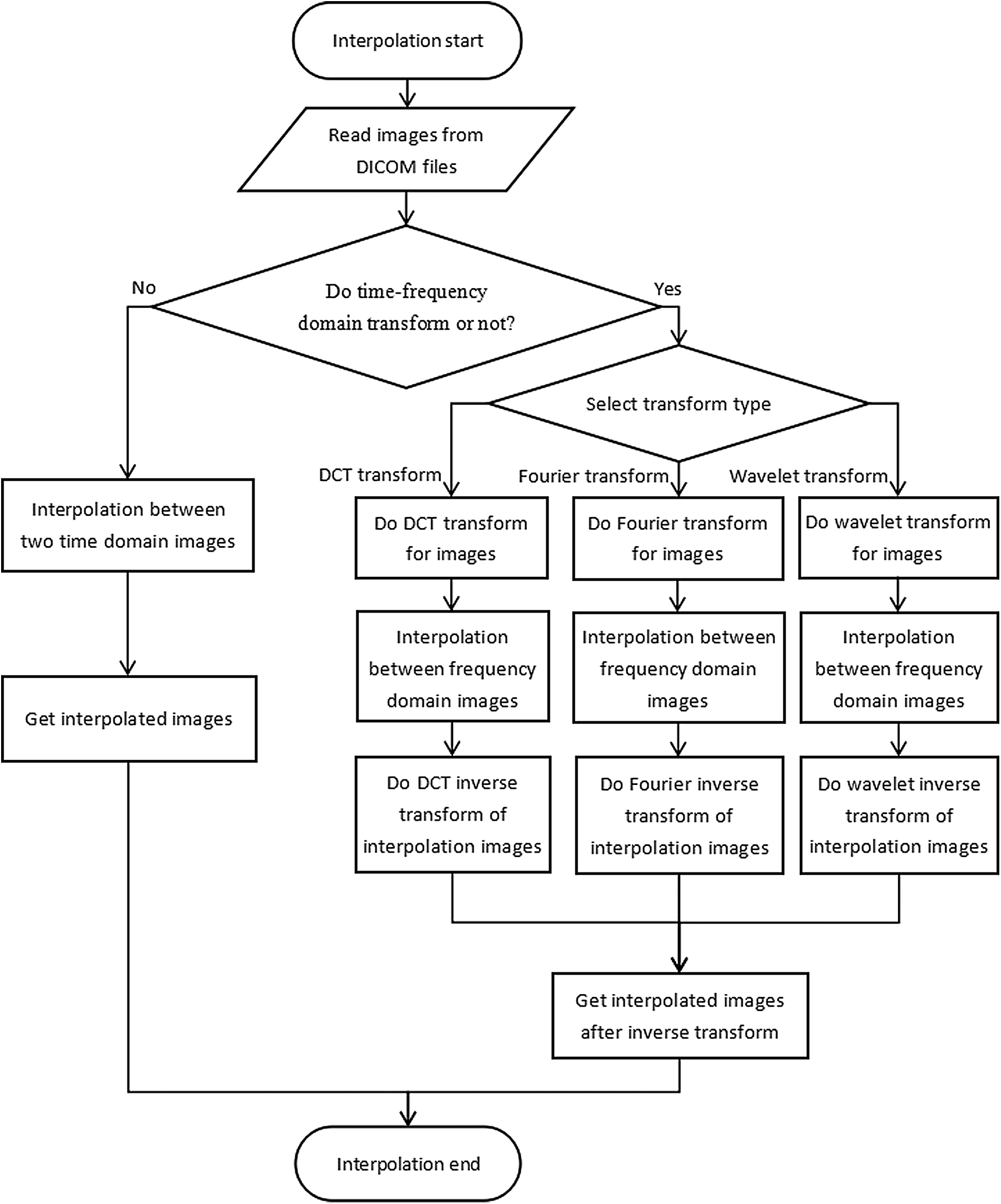
The general method of 3D interpolation in time-frequency domain. 3D, three-dimensional.
3. Three-Dimensional Matching Interpolation Method Based on Wavelet Transform and Sobel Edge Detection
The matching interpolation process is roughly as follows: First, set a matching function to find a set of matching points in the upper and lower two layers of the image. And then find a pair of best matching points in this set of matching points according to the conditions set in advance. Finally, linear interpolation is used to get the gray value of the interpolated image from the gray value of the best matching point. Matching interpolation methods that are commonly used are as follows: a projection point matching method proposed by Denton and Beveridge (2002) matching interpolation by corresponding point, etc.
Traditional matching interpolations are only used in the time-domain interpolation of the image, and they do not use the characteristics and information in the frequency domain. After time-frequency domain transformation, the image can be processed in the frequency domain, and a variety of treatment methods are obtained. Fourier transform and DCT can only get a spectrum, but the wavelet transform can get a time-frequency spectrum. And then we do processing and analysis with a time-frequency spectrum. Wavelet transform makes interpolation of time-frequency domain images at the same time. It is more effective than a direct process with the complete image, and it can overcome the shortcomings of traditional interpolation methods in edge information and texture features.
For the two slice images Zk and Zk+1, we will get a new image Zk+d after making 3D interpolation in the middle place d. In this article, the 3D matching interpolation method based on wavelet transform and Sobel edge detection is mainly divided into the following steps:
(1) Making wavelet transformation with two slice images Zk and Zk+1, we will get a series of wavelet high-frequency sub-images (LHk, HLk, HHk, LHk+1, HLk+1, HHk+1) and wavelet low-frequency sub-images (LLk, LLk+1). (2) Making linear interpolation of high-frequency sub-images, and getting new high-frequency sub-images (LHk+d, HLk+d, HHk+d). (3) Making matching interpolation based on Sobel edge detection of low-frequency sub-images, and getting a new low-frequency sub-image (LLk+d). (4) The high-frequency sub-images (LHk+d, HLk+d, HHk+d) and low-frequency sub-image (LLk+d) mentioned earlier constitute the wavelet sub-image of the interpolation image. We will get the interpolated image by making wavelet inverse transform of these sub-images.
The method is based on wavelet transform, and the Sobel edge detection is integrated into the traditional matching interpolation method. Details of the process are shown in Figure 3.
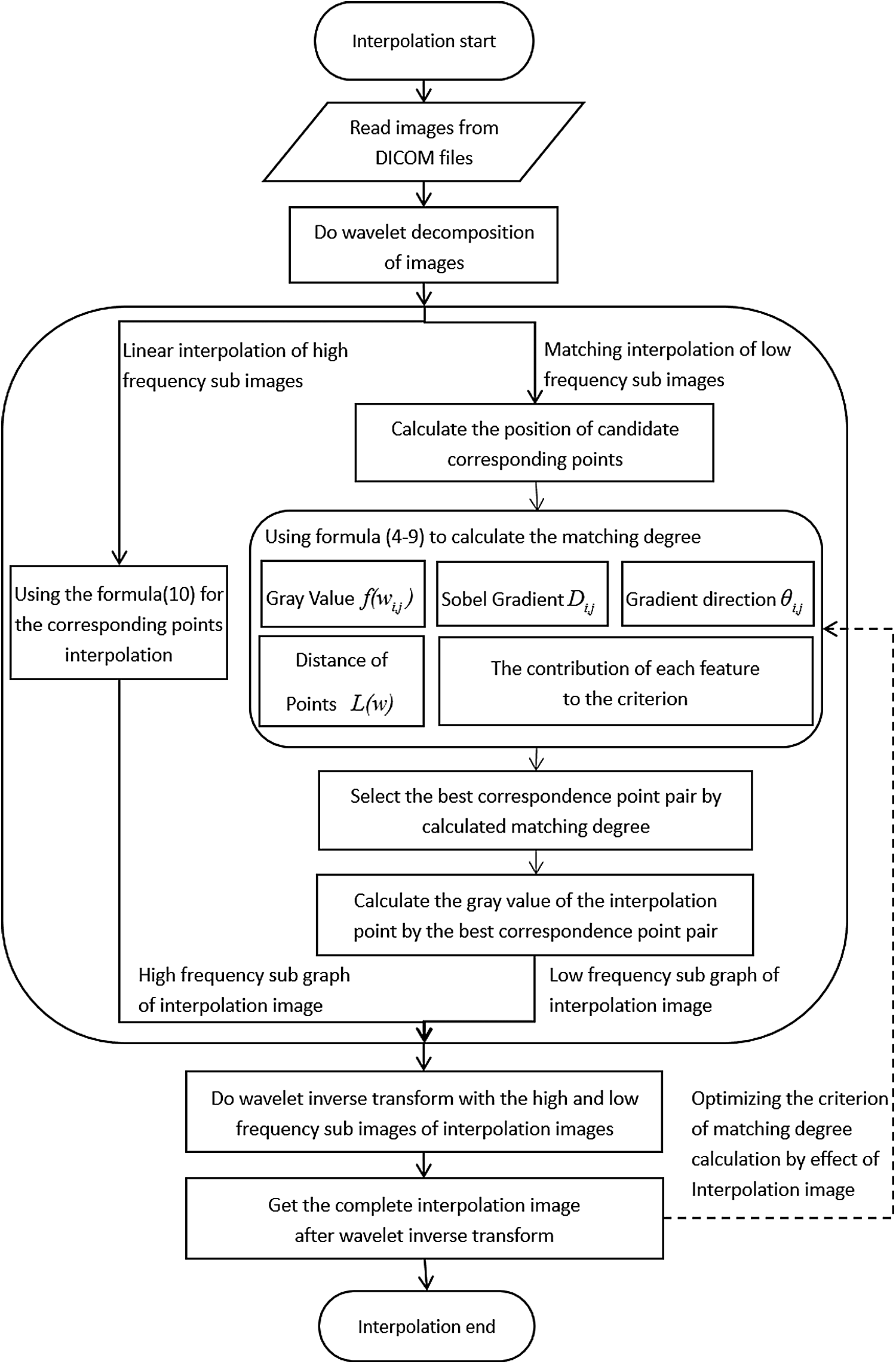
The flow chart of 3D matching interpolation method based on wavelet transform and Sobel edge detection.
There are various wavelet transforms, such as bior, Haar, coif1, sym2, dmey, rbio, and so on. It needs to be verified as to which wavelet transform can achieve a better effect on 3D matching interpolation. In this article, bior3.7, Haar, coif1, sym2, dmey, and rbio3.7 wavelets are selected to decompose and reconstruct the medical image. We will find an appropriate wavelet through the experiment.
Sections 3.1–3.3 give the specific process of the 3D matching interpolation method based on wavelet transform and Sobel edge detection.
3.1. Calculate the position of candidate corresponding points
First, we select the fixed window width W. To ensure the symmetry of the window, the singular value is set as the window width, for example, 3 × 3, 5 × 5, 7 × 7, and so on. Second, as shown in Figure 4, the distance between adjacent layers is d, and we need to establish the gray value of point w(x′,y′,z′) on the middle layer. We can select a point w(x′,y′,zk) on the layer Zk, and connect this point and point w(x′,y′,z′) on the middle layer point with the extension line. This extension line and layer Zk+1 intersect at a point w(x′,y′,zk+1). Point w(x′,y′,zk) and point w(x′,y′,zk+1) constitute the corresponding point pair. With each point in the layer Zk, we can find w2 pairs of candidate corresponding points.
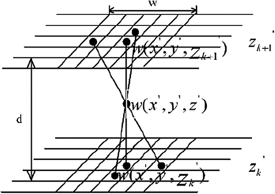
Position of candidate corresponding points of medical image.
3.2. Select the best correspondence point pair
We use a suitable matching criterion to judge candidate corresponding point pairs. The best correspondence point pair is selected by calculating the matching degree. After analysis and improvement, we use the following rules to select the best correspondence point pair:
(1) Gray value f (wi,j) of the point wi,j; (2) Sobel gradient Di,j and gray gradient direction θi,j of the point wi,j; (3) The distance L(w) between pairs of points; (4) Contribution of gray scale, gradient, and gradient direction to the criterion.
Set up the gray value of point wi,j as f (wi,j), the Sobel gradient as Di,j, and the gray gradient direction as θi,j. The calculation formula is as follows:
At the same time, considering that the matching degree between corresponding point pairs is inversely proportional to the distance, the distance exponential distribution function is:
Comprehensively analyze the characteristics of the correspondence point pair, and add the weight λ1 of gray value, the weight λ2 of Sobel gradient, and the weight λ3 of gradient direction. The matching criterion formula is:
When the minimum value of R(i,j,i′,j′) is obtained, the matching degree of the candidate matching point is the highest, and the best matching point is obtained. The value is 0 when the two medical images in the region are of the same pixel value.
3.3. Calculate the gray value of the interpolation point
After getting the best corresponding points wi,j and wi′,j′, we can obtain the gray value of the target interpolation point through their gray value. It is assumed that the variation between the target interpolation point and the best corresponding point pair is linear. Therefore, the gray value f (wx,y) of point wx,y is obtained by the linear interpolation formula. The distance between wx,y and Zk is set as d1, and the distance between wx,y and Zk+1 is d2. The interpolation formula is as follows:
We can get the final image through the interpolation of all points in the target image by using the method described earlier.
4. Results and Analysis
In this section, we use the proposed method and the traditional method to carry out experiments on a series of real medical images, and the interpolation method is evaluated by the following four parameters:
(1) Execution time t(s). (2) Mean-squared difference σ(I
d
), defined as formula (11); among them, M is the total number of points in the original image Iimage, fd(i) is the gray value of the image obtained by interpolation on the position i, and fimage (i) is the gray value of the position i. (3) Number of sites of disagreement β(Id), “a” in formula (13) is a fault tolerance factor. Because interpolation involves a series of floating-point calculations, interpolation of the gray value will be biased. Setting “a” can have the effect of fault tolerance. (4) Sum of absolute deviation of gray value λ(Id).
Among them, the less the execution time t(s) is, the higher the efficiency of the method is. The smaller σ(I d ), β(I d ), and λ(I d ) are, the higher the image and the original image matching degree are obtained.
4.1. Comparison of interpolation result by different transform
In this article, we choose three different types of time-frequency domain transform: DCT, Fourier transform, and wavelet transform. Due to the lack of general methods for 3D interpolation in the frequency domain, we select the linear interpolation method. We do linear interpolation after the transformation of the graph, and the interpolation image is obtained by the inverse transformation. These images are compared with images performing interpolation directly without transformation. We analyze the values of the four indicators mentioned earlier. Table 1 and Figure 5 show the comparison among various interpolation methods.
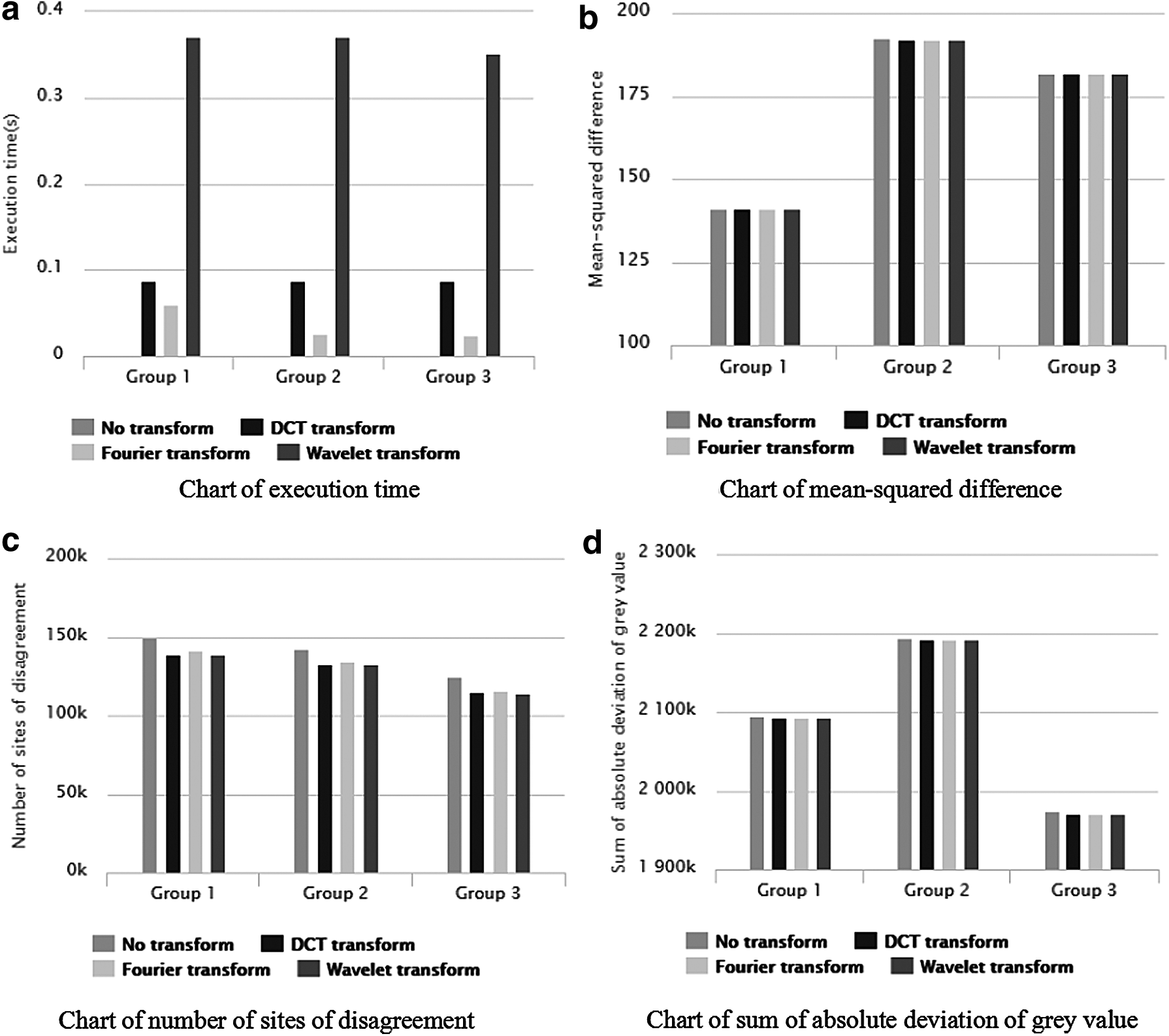
Comparison chart of interpolation result by different transforms.
DCT, discrete cosine transform.
As shown by the experimental results mentioned earlier, interpolation without transformation has a higher running speed, but its effect is the worst. If the 3D interpolation method is not optimized and improved, σ(Id), β(Id), and λ(Id) all have corresponding reductions and improved effects through a variety of different time-frequency domain transformations. The effects do not have many differences among various transformations.
This shows that the time-frequency domain transformation improves the quality of 3D interpolation, and in the frequency domain, there are a variety of image processing methods that can further enhance the quality of interpolation.
Wavelet transform decomposition will obtain four sub-images, which is different from other transformations. We can perform different operations on each sub-image. Low-frequency sub-images roughly have the appearances of original images. Many other interpolation methods can be used in 3D interpolation. Therefore, although the wavelet transform takes more time, its advantage is obvious.
4.2. Comparison of interpolation result by different wavelet transforms
In this article, we selected bior3.7, haar, coif1, sym2, dmey, and rbio3.7 wavelet to decompose and reconstruct tomographic images. With the proposed method, we experiment on two tomographic images. The parameters are set as: λ1 = 1, λ2 = 2, λ3 = 1.
We analyze and compare the values of the four indicators mentioned earlier. Table 2 and Figure 6 are given to compare the interpolation effects with different wavelets.
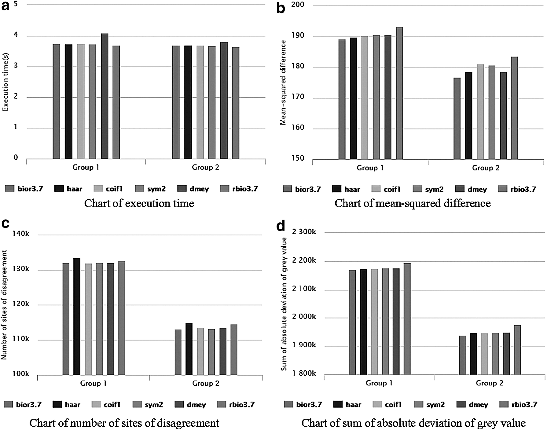
Comparison chart of interpolation result by different wavelet transforms.
From the experimental results mentioned earlier, the execution time of the method using wavelet bior3.7 has the best results on mean-square deviation, gray variance values ranging from the total number of points, and gray value difference of the absolute value of the parameter, although it is not the shortest. Thus, we choose bior3.7 as the wavelet to perform wavelet decomposition and reconstruction.
4.3. Comparison of the proposed method and traditional methods
Experiments are executed with linear interpolation, traditional matching interpolation, and the method proposed in this article on five groups of tomographic images. The parameters of the interpolation method proposed in this article are set as λ1 = 1, λ2 = 2, and λ3 = 1, and bior3.7 wavelet is used. Table 3 and Figure 7 compare our proposed method with the others. It can be seen that in the same experimental image and under the same experimental conditions, the average variance of the proposed method, the total number of pixels, and the absolute value of all gray values are significantly lower than those in the traditional methods. But it takes more time than linear interpolation and traditional matching interpolation.
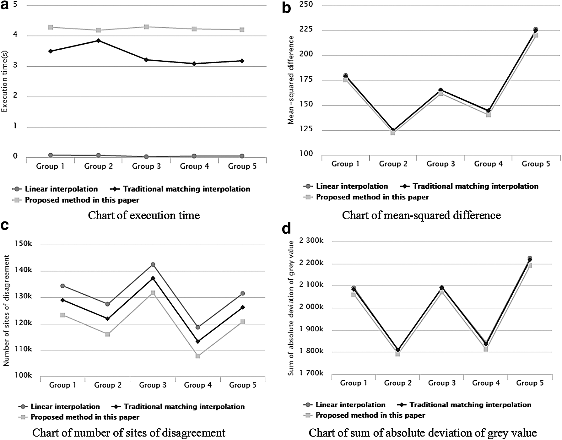
Comparison of interpolation result by different methods.
Figure 8 depicts the results of the fifth group experiments; Figure 8a–c indicates the original images; and Figure 8d–f depicts the effects after various methods of interpolation. Compared with the traditional method, the proposed method has a clear outline of the image that is the closest to the original images.

The interpolation result by different methods.
5. Conclusion
The 3D interpolation of medical images is an important method of improving the image quality in 3D reconstruction. The effect of interpolation directly affects the quality of 3D reconstruction. Thus, it is necessary to design a good interpolation method. In this article, we operate on tomographic images. Sobel edge detection operator and the frequency domain transform are used in 3D matching interpolation. We propose a new interpolation method that combines wavelet transform, Sobel edge detection operator, and 3D matching interpolation together. Experimental results indicate that the mean variance, pixels range point total, and all the gray value difference absolute value are significantly lower than those in several traditional interpolation methods, although the efficiency decreased. This method makes interpolation and image edge clearer and indicates improvements in both visual effects and qualities.
Footnotes
Acknowledgment
This work is partially supported by Shanghai Innovation Action Plan Project under grant No. 16511101200.
Author Disclosure Statement
No competing financial interests exist.