A Poisson Log-Normal Model for Constructing Gene Covariation Network Using RNA-seq Data

2.1. PLN model

In this section, we describe the proposed PLN model for estimating a sparse undirected network using RNA-seq read count data. Let \documentclass{aastex}\usepackage{amsbsy}\usepackage{amsfonts}\usepackage{amssymb}\usepackage{bm}\usepackage{mathrsfs}\usepackage{pifont}\usepackage{stmaryrd}\usepackage{textcomp}\usepackage{portland, xspace}\usepackage{amsmath, amsxtra}\usepackage{upgreek}\pagestyle{empty}\DeclareMathSizes{10}{9}{7}{6}\begin{document} $${ \bf{X}} = { \left[ {{{ \bf{x}}^1} , {{ \bf{x}}^2} , \ldots , {{ \bf{x}}^n}} \right] ^T}$$ \end{document} be an \documentclass{aastex}\usepackage{amsbsy}\usepackage{amsfonts}\usepackage{amssymb}\usepackage{bm}\usepackage{mathrsfs}\usepackage{pifont}\usepackage{stmaryrd}\usepackage{textcomp}\usepackage{portland, xspace}\usepackage{amsmath, amsxtra}\usepackage{upgreek}\pagestyle{empty}\DeclareMathSizes{10}{9}{7}{6}\begin{document} $$n \times d$$ \end{document} matrix representing the observed counts for n samples and d genes. We assume the n samples are independent, and the entries of \documentclass{aastex}\usepackage{amsbsy}\usepackage{amsfonts}\usepackage{amssymb}\usepackage{bm}\usepackage{mathrsfs}\usepackage{pifont}\usepackage{stmaryrd}\usepackage{textcomp}\usepackage{portland, xspace}\usepackage{amsmath, amsxtra}\usepackage{upgreek}\pagestyle{empty}\DeclareMathSizes{10}{9}{7}{6}\begin{document} $${{ \bf{x}}^i} = ( x_1^i , \cdots , x_d^i{ ) ^T}$$ \end{document} are conditionally independent, given the underlying unobserved expression levels of the ith sample whose logarithm is denoted by \documentclass{aastex}\usepackage{amsbsy}\usepackage{amsfonts}\usepackage{amssymb}\usepackage{bm}\usepackage{mathrsfs}\usepackage{pifont}\usepackage{stmaryrd}\usepackage{textcomp}\usepackage{portland, xspace}\usepackage{amsmath, amsxtra}\usepackage{upgreek}\pagestyle{empty}\DeclareMathSizes{10}{9}{7}{6}\begin{document} $${ \bm{\eta} ^i} = ( \eta _1^i , \cdots , \eta _d^i{ ) ^T}$$ \end{document} .

We assume that for \documentclass{aastex}\usepackage{amsbsy}\usepackage{amsfonts}\usepackage{amssymb}\usepackage{bm}\usepackage{mathrsfs}\usepackage{pifont}\usepackage{stmaryrd}\usepackage{textcomp}\usepackage{portland, xspace}\usepackage{amsmath, amsxtra}\usepackage{upgreek}\pagestyle{empty}\DeclareMathSizes{10}{9}{7}{6}\begin{document} $$i = 1 , \cdots , n$$ \end{document} \documentclass{aastex}\usepackage{amsbsy}\usepackage{amsfonts}\usepackage{amssymb}\usepackage{bm}\usepackage{mathrsfs}\usepackage{pifont}\usepackage{stmaryrd}\usepackage{textcomp}\usepackage{portland, xspace}\usepackage{amsmath, amsxtra}\usepackage{upgreek}\pagestyle{empty}\DeclareMathSizes{10}{9}{7}{6}\begin{document} \begin{align*} x_j^i \vert { \bm{\eta} ^i} \mathop \sim \limits^{{ \rm{indep}}} {{ \rm Poisson}} ( {K^i} \exp ( \eta _j^i ) ) , \ j = 1 , \cdots , d , \end{align*} \end{document}

where Kⁱ is a scaling factor adjusting for library size of the ith sample. Although the observed counts of mapped reads also depend on the length of the gene, it is equivalent and notationally more convenient to account for this factor in \documentclass{aastex}\usepackage{amsbsy}\usepackage{amsfonts}\usepackage{amssymb}\usepackage{bm}\usepackage{mathrsfs}\usepackage{pifont}\usepackage{stmaryrd}\usepackage{textcomp}\usepackage{portland, xspace}\usepackage{amsmath, amsxtra}\usepackage{upgreek}\pagestyle{empty}\DeclareMathSizes{10}{9}{7}{6}\begin{document} $$\eta _j^i$$ \end{document} , because the length is constant for each gene across all samples. We further assume that the underlying expression levels follow a multivariate log-normal distribution, that is, \documentclass{aastex}\usepackage{amsbsy}\usepackage{amsfonts}\usepackage{amssymb}\usepackage{bm}\usepackage{mathrsfs}\usepackage{pifont}\usepackage{stmaryrd}\usepackage{textcomp}\usepackage{portland, xspace}\usepackage{amsmath, amsxtra}\usepackage{upgreek}\pagestyle{empty}\DeclareMathSizes{10}{9}{7}{6}\begin{document} \begin{align*} {{\mathbf{\eta}}^i} \mathop \sim \limits^{{ \rm{i}}{ \rm{.i}}{ \rm{.d}}{ \rm{.}}} N ({\mathbf{\mu}} , {\mathbf{\Sigma}}) , i = 1 , \cdots , n. \end{align*} \end{document}

Under the mentioned model, denoting \documentclass{aastex}\usepackage{amsbsy}\usepackage{amsfonts}\usepackage{amssymb}\usepackage{bm}\usepackage{mathrsfs}\usepackage{pifont}\usepackage{stmaryrd}\usepackage{textcomp}\usepackage{portland, xspace}\usepackage{amsmath, amsxtra}\usepackage{upgreek}\pagestyle{empty}\DeclareMathSizes{10}{9}{7}{6}\begin{document} $${ \bf{A}} = { \mathbf{\Sigma} ^{ - 1}}$$ \end{document} and using \documentclass{aastex}\usepackage{amsbsy}\usepackage{amsfonts}\usepackage{amssymb}\usepackage{bm}\usepackage{mathrsfs}\usepackage{pifont}\usepackage{stmaryrd}\usepackage{textcomp}\usepackage{portland, xspace}\usepackage{amsmath, amsxtra}\usepackage{upgreek}\pagestyle{empty}\DeclareMathSizes{10}{9}{7}{6}\begin{document} $$p ( \cdot )$$ \end{document} as a generic symbol for probability density function, the likelihood function is \documentclass{aastex}\usepackage{amsbsy}\usepackage{amsfonts}\usepackage{amssymb}\usepackage{bm}\usepackage{mathrsfs}\usepackage{pifont}\usepackage{stmaryrd}\usepackage{textcomp}\usepackage{portland, xspace}\usepackage{amsmath, amsxtra}\usepackage{upgreek}\pagestyle{empty}\DeclareMathSizes{10}{9}{7}{6}\begin{document} $$L(\mathbf{\mu} , {\textbf{{A}}}) = \prod_{i = 1}^n {L_i} ( {\mathbf{\mu}} , {\textbf{{A}}} )$$ \end{document} , where \documentclass{aastex}\usepackage{amsbsy}\usepackage{amsfonts}\usepackage{amssymb}\usepackage{bm}\usepackage{mathrsfs}\usepackage{pifont}\usepackage{stmaryrd}\usepackage{textcomp}\usepackage{portland, xspace}\usepackage{amsmath, amsxtra}\usepackage{upgreek}\pagestyle{empty}\DeclareMathSizes{10}{9}{7}{6}\begin{document} \begin{align*} & { L_i } ( {\mathbf {\mu}} , { \bf{ A } } ) = { p_ { { { \bf { X } } ^i } } } ( { { \bf { x } } ^i } ) = \int_ { { { \bf { R } } ^d } } { p_ { { { \bf { X } } ^i } \vert { \mathbf {\eta} ^i } } } ( { { \bf { x } } ^i } ) { p_ { \eta } } ( { { \eta } ^i } ) d { { \eta } ^i } \\ & \quad \quad \quad \; \; = \int_ { { { \bf { R } } ^d } } (2 \pi)^{- \frac {d} {2}} | { \textbf{ { A }} } { | ^ {\frac { 1 } { 2 }}} \exp \left( { - \frac { 1 } { 2 } { { ( { { \eta } ^i } - { \mu } ) } ^T } { \bf { A } } ( { { \eta } ^i } - { \mu } ) } \right) \prod \limits_ { j = 1 } ^d { e^ { - { K^i } { e^ { \eta _j^i } } } } { \frac { { { \left( { { K^i } { e^ { \eta _j^i } } } \right) } ^ { x_j^i } } } { x_j^i! } } d { { \eta } ^i } . \tag { 1 } \end{align*} \end{document}

Our goal is to estimate the concentration matrix, \documentclass{aastex}\usepackage{amsbsy}\usepackage{amsfonts}\usepackage{amssymb}\usepackage{bm}\usepackage{mathrsfs}\usepackage{pifont}\usepackage{stmaryrd}\usepackage{textcomp}\usepackage{portland, xspace}\usepackage{amsmath, amsxtra}\usepackage{upgreek}\pagestyle{empty}\DeclareMathSizes{10}{9}{7}{6}\begin{document} $${ \bf{A}};$$ \end{document} in particular, we aim to identify nonzero entries of \documentclass{aastex}\usepackage{amsbsy}\usepackage{amsfonts}\usepackage{amssymb}\usepackage{bm}\usepackage{mathrsfs}\usepackage{pifont}\usepackage{stmaryrd}\usepackage{textcomp}\usepackage{portland, xspace}\usepackage{amsmath, amsxtra}\usepackage{upgreek}\pagestyle{empty}\DeclareMathSizes{10}{9}{7}{6}\begin{document} $${ \bf{A}} ,$$ \end{document} which indicate conditionally covarying pairs of genes. The Gaussian mean parameter, \documentclass{aastex}\usepackage{amsbsy}\usepackage{amsfonts}\usepackage{amssymb}\usepackage{bm}\usepackage{mathrsfs}\usepackage{pifont}\usepackage{stmaryrd}\usepackage{textcomp}\usepackage{portland, xspace}\usepackage{amsmath, amsxtra}\usepackage{upgreek}\pagestyle{empty}\DeclareMathSizes{10}{9}{7}{6}\begin{document} $$\bm{\mu} ,$$ \end{document} is treated as a nuisance parameter. The scaling factors, Kⁱ, are assumed to be known constants. To encourage sparsity, we seek a positive definite \documentclass{aastex}\usepackage{amsbsy}\usepackage{amsfonts}\usepackage{amssymb}\usepackage{bm}\usepackage{mathrsfs}\usepackage{pifont}\usepackage{stmaryrd}\usepackage{textcomp}\usepackage{portland, xspace}\usepackage{amsmath, amsxtra}\usepackage{upgreek}\pagestyle{empty}\DeclareMathSizes{10}{9}{7}{6}\begin{document} $${ \bf{A}}$$ \end{document} that minimizes an \documentclass{aastex}\usepackage{amsbsy}\usepackage{amsfonts}\usepackage{amssymb}\usepackage{bm}\usepackage{mathrsfs}\usepackage{pifont}\usepackage{stmaryrd}\usepackage{textcomp}\usepackage{portland, xspace}\usepackage{amsmath, amsxtra}\usepackage{upgreek}\pagestyle{empty}\DeclareMathSizes{10}{9}{7}{6}\begin{document} $${ \ell _1}$$ \end{document} penalized log-likelihood function: \documentclass{aastex}\usepackage{amsbsy}\usepackage{amsfonts}\usepackage{amssymb}\usepackage{bm}\usepackage{mathrsfs}\usepackage{pifont}\usepackage{stmaryrd}\usepackage{textcomp}\usepackage{portland, xspace}\usepackage{amsmath, amsxtra}\usepackage{upgreek}\pagestyle{empty}\DeclareMathSizes{10}{9}{7}{6}\begin{document} \begin{align*} O ( \bm { \mu } , { \bf { A } } ) = - \frac { 1 } { n } \mathop \sum \limits_ { i = 1 } ^n \log ( { L_i } ( \bm { \mu } , { \bf { A } } ) ) + \lambda \mathop \sum \limits_ { j \ne k } \; { W_ { jk } } \vert { A_ { jk } } \vert , \tag { 2 } \end{align*} \end{document}

where \documentclass{aastex}\usepackage{amsbsy}\usepackage{amsfonts}\usepackage{amssymb}\usepackage{bm}\usepackage{mathrsfs}\usepackage{pifont}\usepackage{stmaryrd}\usepackage{textcomp}\usepackage{portland, xspace}\usepackage{amsmath, amsxtra}\usepackage{upgreek}\pagestyle{empty}\DeclareMathSizes{10}{9}{7}{6}\begin{document} $${W_{jk}}$$ \end{document} is a weight that allows differential amounts of regularization of the entries of \documentclass{aastex}\usepackage{amsbsy}\usepackage{amsfonts}\usepackage{amssymb}\usepackage{bm}\usepackage{mathrsfs}\usepackage{pifont}\usepackage{stmaryrd}\usepackage{textcomp}\usepackage{portland, xspace}\usepackage{amsmath, amsxtra}\usepackage{upgreek}\pagestyle{empty}\DeclareMathSizes{10}{9}{7}{6}\begin{document} $${ \bf{A}}$$ \end{document} based on prior knowledge or anticipated network properties (see Supplementary Data).

2.2. Computational algorithm

Optimization of the objective function in Equation (2) is computationally prohibitive because each evaluation of the likelihood function requires a d-dimensional integration, which does not have a closed form solution. Our strategy is to use Laplace's method of integration, which enables us to approximate the objective function [Eq. (2)] in closed form (up to a constant that does not involve unknown parameters): \documentclass{aastex}\usepackage{amsbsy}\usepackage{amsfonts}\usepackage{amssymb}\usepackage{bm}\usepackage{mathrsfs}\usepackage{pifont}\usepackage{stmaryrd}\usepackage{textcomp}\usepackage{portland, xspace}\usepackage{amsmath, amsxtra}\usepackage{upgreek}\pagestyle{empty}\DeclareMathSizes{10}{9}{7}{6}\begin{document} \begin{align*} & O ( \bm { \mu } , { \bf { A } } ) \approx - \frac { 1 } { 2 } \log \vert { \bf { A } } \vert + \frac { 1 } { { 2n } } \mathop \sum \limits_ { i = 1 } ^n { ( { \bm { \eta } ^ { * ( i ) } } - \bm { \mu } ) ^T } { \bf { A } } ( { \eta ^ { * ( i ) } } - \mu ) + \frac { { 1 } } { n } \mathop \sum \limits_ { i = 1 } ^n \left[ { { K^i } { { \bf { 1 } } ^T } { e^ { { \bm { \eta } ^ { * ( i ) } } } } - { \bm { \eta } ^ { * ( i ) T } } { { \bf { x } } ^i } } \right] \\ & \quad \quad \quad + \frac { 1 } { { 2n } } \mathop \sum \limits_ { i = 1 } ^n \log \left\vert { { \rm { diag } } \left( { { K^i } { e^ { { \eta ^ { * ( i ) } } } } } \right) + { \bf { A } } } \right\vert + \lambda \mathop \sum \limits_ { j \ne k } \; { W_ { jk } } \vert { A_ { jk } } \vert , \tag { 3 } \end{align*} \end{document}

where \documentclass{aastex}\usepackage{amsbsy}\usepackage{amsfonts}\usepackage{amssymb}\usepackage{bm}\usepackage{mathrsfs}\usepackage{pifont}\usepackage{stmaryrd}\usepackage{textcomp}\usepackage{portland, xspace}\usepackage{amsmath, amsxtra}\usepackage{upgreek}\pagestyle{empty}\DeclareMathSizes{10}{9}{7}{6}\begin{document} $${\bm{\eta}^{*(i)}} = arg \ max_{{\bm{\eta}^i}} log {p_{{{ \bf{X}}^i} | {\bm{\eta}^i}}} ({{\bf{x}}^i}) {p_{\bm{\eta}}} ({ \bm{\eta}^i} )$$ \end{document} .

To obtain parameter estimates that minimize the objective function, we alternatively update \documentclass{aastex}\usepackage{amsbsy}\usepackage{amsfonts}\usepackage{amssymb}\usepackage{bm}\usepackage{mathrsfs}\usepackage{pifont}\usepackage{stmaryrd}\usepackage{textcomp}\usepackage{portland, xspace}\usepackage{amsmath, amsxtra}\usepackage{upgreek}\pagestyle{empty}\DeclareMathSizes{10}{9}{7}{6}\begin{document} $${ \bm{\eta} ^{* ( i ) }}$$ \end{document} for fixed \documentclass{aastex}\usepackage{amsbsy}\usepackage{amsfonts}\usepackage{amssymb}\usepackage{bm}\usepackage{mathrsfs}\usepackage{pifont}\usepackage{stmaryrd}\usepackage{textcomp}\usepackage{portland, xspace}\usepackage{amsmath, amsxtra}\usepackage{upgreek}\pagestyle{empty}\DeclareMathSizes{10}{9}{7}{6}\begin{document} $$( \bm{\mu} , { \bf{A}} )$$ \end{document} using Newton's method, and update \documentclass{aastex}\usepackage{amsbsy}\usepackage{amsfonts}\usepackage{amssymb}\usepackage{bm}\usepackage{mathrsfs}\usepackage{pifont}\usepackage{stmaryrd}\usepackage{textcomp}\usepackage{portland, xspace}\usepackage{amsmath, amsxtra}\usepackage{upgreek}\pagestyle{empty}\DeclareMathSizes{10}{9}{7}{6}\begin{document} $$\bm{\mu}$$ \end{document} and \documentclass{aastex}\usepackage{amsbsy}\usepackage{amsfonts}\usepackage{amssymb}\usepackage{bm}\usepackage{mathrsfs}\usepackage{pifont}\usepackage{stmaryrd}\usepackage{textcomp}\usepackage{portland, xspace}\usepackage{amsmath, amsxtra}\usepackage{upgreek}\pagestyle{empty}\DeclareMathSizes{10}{9}{7}{6}\begin{document} $${ \bf{A}}$$ \end{document} given \documentclass{aastex}\usepackage{amsbsy}\usepackage{amsfonts}\usepackage{amssymb}\usepackage{bm}\usepackage{mathrsfs}\usepackage{pifont}\usepackage{stmaryrd}\usepackage{textcomp}\usepackage{portland, xspace}\usepackage{amsmath, amsxtra}\usepackage{upgreek}\pagestyle{empty}\DeclareMathSizes{10}{9}{7}{6}\begin{document} $${ \bm{\eta} ^{* ( i ) }}$$ \end{document} using an ADMM algorithm (Boyd et al., 2011). Finally, the tuning parameter \documentclass{aastex}\usepackage{amsbsy}\usepackage{amsfonts}\usepackage{amssymb}\usepackage{bm}\usepackage{mathrsfs}\usepackage{pifont}\usepackage{stmaryrd}\usepackage{textcomp}\usepackage{portland, xspace}\usepackage{amsmath, amsxtra}\usepackage{upgreek}\pagestyle{empty}\DeclareMathSizes{10}{9}{7}{6}\begin{document} $$\lambda$$ \end{document} , which controls the sparsity of the inferred network, is chosen by the extended Bayesian information criterion (eBIC) criterion (Chen and Chen, 2008). Details about the approximation and optimization of the objective function can be found in Supplementary Data.

2.3. Simulation studies

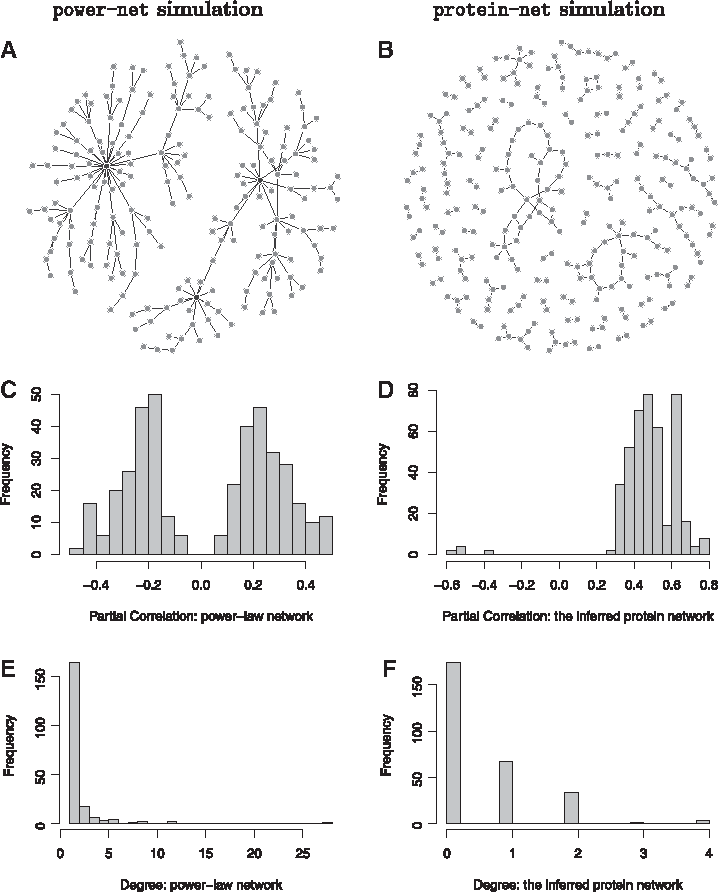
We conduct a series of simulation studies to compare the PLN and GGM approaches. Counts data are generated in the following way: we start with an assumed graph, which either follows a power-law network (Newman, 2003) or an inferred protein network (Wu et al., 2013). The mean expression level, \documentclass{aastex}\usepackage{amsbsy}\usepackage{amsfonts}\usepackage{amssymb}\usepackage{bm}\usepackage{mathrsfs}\usepackage{pifont}\usepackage{stmaryrd}\usepackage{textcomp}\usepackage{portland, xspace}\usepackage{amsmath, amsxtra}\usepackage{upgreek}\pagestyle{empty}\DeclareMathSizes{10}{9}{7}{6}\begin{document} $$\mu$$ \end{document} , and the concentration matrix, A, are generated according to the connectivity of the graph and a prespecified distribution that controls the signal-to-noise ratio (Fig. 1C). Next, the latent expression level \documentclass{aastex}\usepackage{amsbsy}\usepackage{amsfonts}\usepackage{amssymb}\usepackage{bm}\usepackage{mathrsfs}\usepackage{pifont}\usepackage{stmaryrd}\usepackage{textcomp}\usepackage{portland, xspace}\usepackage{amsmath, amsxtra}\usepackage{upgreek}\pagestyle{empty}\DeclareMathSizes{10}{9}{7}{6}\begin{document} $$( \bm{\eta} )$$ \end{document} and the observed counts \documentclass{aastex}\usepackage{amsbsy}\usepackage{amsfonts}\usepackage{amssymb}\usepackage{bm}\usepackage{mathrsfs}\usepackage{pifont}\usepackage{stmaryrd}\usepackage{textcomp}\usepackage{portland, xspace}\usepackage{amsmath, amsxtra}\usepackage{upgreek}\pagestyle{empty}\DeclareMathSizes{10}{9}{7}{6}\begin{document} $${ \bf{x}}$$ \end{document} are simulated according to the PLN model described in Section 2.1. The simulation settings are summarized in Table 1; the details of each simulation can be found in Supplementary Data.

OPEN IN VIEWER

FIG. 1.

(A) The power-law network. (B) The protein network. (C, D) The histograms of partial correlations for power-net simulation and protein-net simulation, respectively. (E, F) The degree distributions for power-law network and protein network, respectively.

For comparison, we apply the graphical lasso (Friedman et al., 2008) to the raw count data as well as to data under several commonly used transformations: (i) normal quantile transformation, (ii) logarithmic transformation, and (iii) square-root transformation. Note that the quantile transformation assigns the same value for ties; thus the transformed data are not guaranteed to be perfectly normal if the data include many ties. Because the counts can be 0 for low-abundance genes, we add 1 to all counts before applying the logarithm transformation.

Although studies of inferring biological networks have primarily focused on edge detection, that is, whether an edge is present or not, the signs and magnitudes of the partial correlations provide clues regarding the nature of the corresponding regulation relationships: positive or negative, strong or weak. Therefore, in addition to edge detection ability, we also compare the \documentclass{aastex}\usepackage{amsbsy}\usepackage{amsfonts}\usepackage{amssymb}\usepackage{bm}\usepackage{mathrsfs}\usepackage{pifont}\usepackage{stmaryrd}\usepackage{textcomp}\usepackage{portland, xspace}\usepackage{amsmath, amsxtra}\usepackage{upgreek}\pagestyle{empty}\DeclareMathSizes{10}{9}{7}{6}\begin{document} $${ \ell _2}$$ \end{document} distance between the estimated and the true partial correlations: \documentclass{aastex}\usepackage{amsbsy}\usepackage{amsfonts}\usepackage{amssymb}\usepackage{bm}\usepackage{mathrsfs}\usepackage{pifont}\usepackage{stmaryrd}\usepackage{textcomp}\usepackage{portland, xspace}\usepackage{amsmath, amsxtra}\usepackage{upgreek}\pagestyle{empty}\DeclareMathSizes{10}{9}{7}{6}\begin{document} \begin{align*} d (\bm{\rho} , \hat {\bm{\rho}} ) = \sqrt { \mathop \sum \limits_{1 \le i , j \le d} \vert { \rho ^{ij}} - {{ \hat \rho }^{ij}}{ | ^2}}. \end{align*} \end{document}

2.4. Application to RNA-seq data

The Geuvadis data consist of RNA-seq assays on 462 lymphoblastoid cell lines derived from five populations: European American from Utah (CEU), Finnish (FIN), British (GBR), Toscani (TSI), and African (Yoruban from Nigeria, YRI) in the 1000 Genomes Project (Lappalainen et al., 2013). We prefilter the data to focus on the 275 genes that overlap with the inferred protein network (Wu et al., 2013). To apply the PLN model and GGMs, we choose to use the RPKM (reads per kilobase of transcript per million mapped reads.), instead of the raw reads, primarily for two reasons: first, RPKM removes some systematic effects such as the batch effects and is the commonly shared form of data. Moreover, it is not always possible to reconstruct the raw read counts from RPKM. Second, empirically, we find both PLN and GGMs lead to more interpretable networks when applied to RPKM reads than to the raw reads. Three existing GGMs are used to analyze the quantile-transformed data on RPKM: (i) neighborhood selection (Meinshausen and Bühlmann, 2006), (ii) space (Peng et al., 2009), and (iii) graphical lasso (Friedman et al., 2008). The RNA-seq expression networks are inferred separately in European (CEU, FIN, GBR, and TSI; total \documentclass{aastex}\usepackage{amsbsy}\usepackage{amsfonts}\usepackage{amssymb}\usepackage{bm}\usepackage{mathrsfs}\usepackage{pifont}\usepackage{stmaryrd}\usepackage{textcomp}\usepackage{portland, xspace}\usepackage{amsmath, amsxtra}\usepackage{upgreek}\pagestyle{empty}\DeclareMathSizes{10}{9}{7}{6}\begin{document} $${\rm N} = 373$$ \end{document} ) and African (YRI, \documentclass{aastex}\usepackage{amsbsy}\usepackage{amsfonts}\usepackage{amssymb}\usepackage{bm}\usepackage{mathrsfs}\usepackage{pifont}\usepackage{stmaryrd}\usepackage{textcomp}\usepackage{portland, xspace}\usepackage{amsmath, amsxtra}\usepackage{upgreek}\pagestyle{empty}\DeclareMathSizes{10}{9}{7}{6}\begin{document} $${\rm N} = 89$$ \end{document} ) populations. For the PLN model, the tuning parameters are selected by minimizing the eBIC with \documentclass{aastex}\usepackage{amsbsy}\usepackage{amsfonts}\usepackage{amssymb}\usepackage{bm}\usepackage{mathrsfs}\usepackage{pifont}\usepackage{stmaryrd}\usepackage{textcomp}\usepackage{portland, xspace}\usepackage{amsmath, amsxtra}\usepackage{upgreek}\pagestyle{empty}\DeclareMathSizes{10}{9}{7}{6}\begin{document} $$\gamma = 0.5$$ \end{document} ; for the three GGMs, tuning parameters are adjusted so that the same number of edges are selected by all methods.

Since there is no known truth to evaluate the performance of these methods on real data, we use the modularity of the constructed network as a surrogate criterion. Each gene is assigned a functional category based on gene ontology (GO). Following Clauset et al. (2004), we define modularity as the fraction of the edges that connect two genes in the same functional category minus the expected value of such fraction if edges were distributed at random. This measure ranges between \documentclass{aastex}\usepackage{amsbsy}\usepackage{amsfonts}\usepackage{amssymb}\usepackage{bm}\usepackage{mathrsfs}\usepackage{pifont}\usepackage{stmaryrd}\usepackage{textcomp}\usepackage{portland, xspace}\usepackage{amsmath, amsxtra}\usepackage{upgreek}\pagestyle{empty}\DeclareMathSizes{10}{9}{7}{6}\begin{document} $$- 1$$ \end{document} and 1, with higher positive values suggesting coordinated regulation of genes in related biological pathways. In practice, a modularity greater than \documentclass{aastex}\usepackage{amsbsy}\usepackage{amsfonts}\usepackage{amssymb}\usepackage{bm}\usepackage{mathrsfs}\usepackage{pifont}\usepackage{stmaryrd}\usepackage{textcomp}\usepackage{portland, xspace}\usepackage{amsmath, amsxtra}\usepackage{upgreek}\pagestyle{empty}\DeclareMathSizes{10}{9}{7}{6}\begin{document} $$0.3$$ \end{document} is taken as an indicator of significant group structure in a network (Clauset et al., 2004).

3.1. Simulation studies

We carry out simulation studies to assess the performance of the PLN model; as comparisons, we compare this model with graphical lasso applied to the raw or transformed count data (Friedman et al., 2008). Other GGM methods, such as neighborhood selection and space (Meinshausen and Bühlmann, 2006; Peng et al., 2009), are also investigated, both of which show similar results as graphical lasso (results not shown).

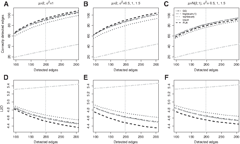
Figures 2 and 3 report the number of correctly detected edges versus the number of total detected edges, averaged across 50 independent replicates with sample size \documentclass{aastex}\usepackage{amsbsy}\usepackage{amsfonts}\usepackage{amssymb}\usepackage{bm}\usepackage{mathrsfs}\usepackage{pifont}\usepackage{stmaryrd}\usepackage{textcomp}\usepackage{portland, xspace}\usepackage{amsmath, amsxtra}\usepackage{upgreek}\pagestyle{empty}\DeclareMathSizes{10}{9}{7}{6}\begin{document} $$n = 100$$ \end{document} . A common pattern shared by all methods is that the power of edge detection improves with the increase of the overall abundance of gene expression levels (large \documentclass{aastex}\usepackage{amsbsy}\usepackage{amsfonts}\usepackage{amssymb}\usepackage{bm}\usepackage{mathrsfs}\usepackage{pifont}\usepackage{stmaryrd}\usepackage{textcomp}\usepackage{portland, xspace}\usepackage{amsmath, amsxtra}\usepackage{upgreek}\pagestyle{empty}\DeclareMathSizes{10}{9}{7}{6}\begin{document} $${ \mu _j}$$ \end{document} ). When the observed counts are very low with many 0's (small \documentclass{aastex}\usepackage{amsbsy}\usepackage{amsfonts}\usepackage{amssymb}\usepackage{bm}\usepackage{mathrsfs}\usepackage{pifont}\usepackage{stmaryrd}\usepackage{textcomp}\usepackage{portland, xspace}\usepackage{amsmath, amsxtra}\usepackage{upgreek}\pagestyle{empty}\DeclareMathSizes{10}{9}{7}{6}\begin{document} $${ \mu _j}$$ \end{document} ), there is little information and all methods perform poorly. Measured in terms of sensitivity and specificity of edge detection, PLN performs comparably to graphical lasso on logarithm- or quantile-transformed data. All methods perform significantly better than applying graphical lasso to the raw counts directly. In addition, the performance of graphical lasso on raw or square-root transformed counts is highly sensitive to the skewness of the data and deteriorates as the variance increases (Fig. 3B, D). In contrast, PLN and graphical lasso with quantile or logarithm transformations are reasonably robust to extreme values in the data; in fact, for a fixed mean expression level, the edge-detection power of these methods improves for more skewed data with higher variance (Fig. 3B, D). Finally, Figure 2 indicates that PLN outperforms all the other methods in terms of estimating the magnitudes of the partial correlations, measured by entry-wise \documentclass{aastex}\usepackage{amsbsy}\usepackage{amsfonts}\usepackage{amssymb}\usepackage{bm}\usepackage{mathrsfs}\usepackage{pifont}\usepackage{stmaryrd}\usepackage{textcomp}\usepackage{portland, xspace}\usepackage{amsmath, amsxtra}\usepackage{upgreek}\pagestyle{empty}\DeclareMathSizes{10}{9}{7}{6}\begin{document} $${ \ell _2}$$ \end{document} distance.

OPEN IN VIEWER

FIG. 2.

Power-net simulation 1. (A–C) The number of total detected edges (x-axis) and the number of correctly detected edges (y-axis) under the three scenarios of \documentclass{aastex}\usepackage{amsbsy}\usepackage{amsfonts}\usepackage{amssymb}\usepackage{bm}\usepackage{mathrsfs}\usepackage{pifont}\usepackage{stmaryrd}\usepackage{textcomp}\usepackage{portland, xspace}\usepackage{amsmath, amsxtra}\usepackage{upgreek}\pagestyle{empty}\DeclareMathSizes{10}{9}{7}{6}\begin{document} $$( { \mu _j} , { \Sigma _{jj}} )$$ \end{document} . (D–F) \documentclass{aastex}\usepackage{amsbsy}\usepackage{amsfonts}\usepackage{amssymb}\usepackage{bm}\usepackage{mathrsfs}\usepackage{pifont}\usepackage{stmaryrd}\usepackage{textcomp}\usepackage{portland, xspace}\usepackage{amsmath, amsxtra}\usepackage{upgreek}\pagestyle{empty}\DeclareMathSizes{10}{9}{7}{6}\begin{document} $${ \ell _2}$$ \end{document} distance (y-axis) between the estimated and the true partial correlations under the three scenarios of \documentclass{aastex}\usepackage{amsbsy}\usepackage{amsfonts}\usepackage{amssymb}\usepackage{bm}\usepackage{mathrsfs}\usepackage{pifont}\usepackage{stmaryrd}\usepackage{textcomp}\usepackage{portland, xspace}\usepackage{amsmath, amsxtra}\usepackage{upgreek}\pagestyle{empty}\DeclareMathSizes{10}{9}{7}{6}\begin{document} $$( { \mu _j} , { \Sigma _{jj}} )$$ \end{document} .

OPEN IN VIEWER

FIG. 3.

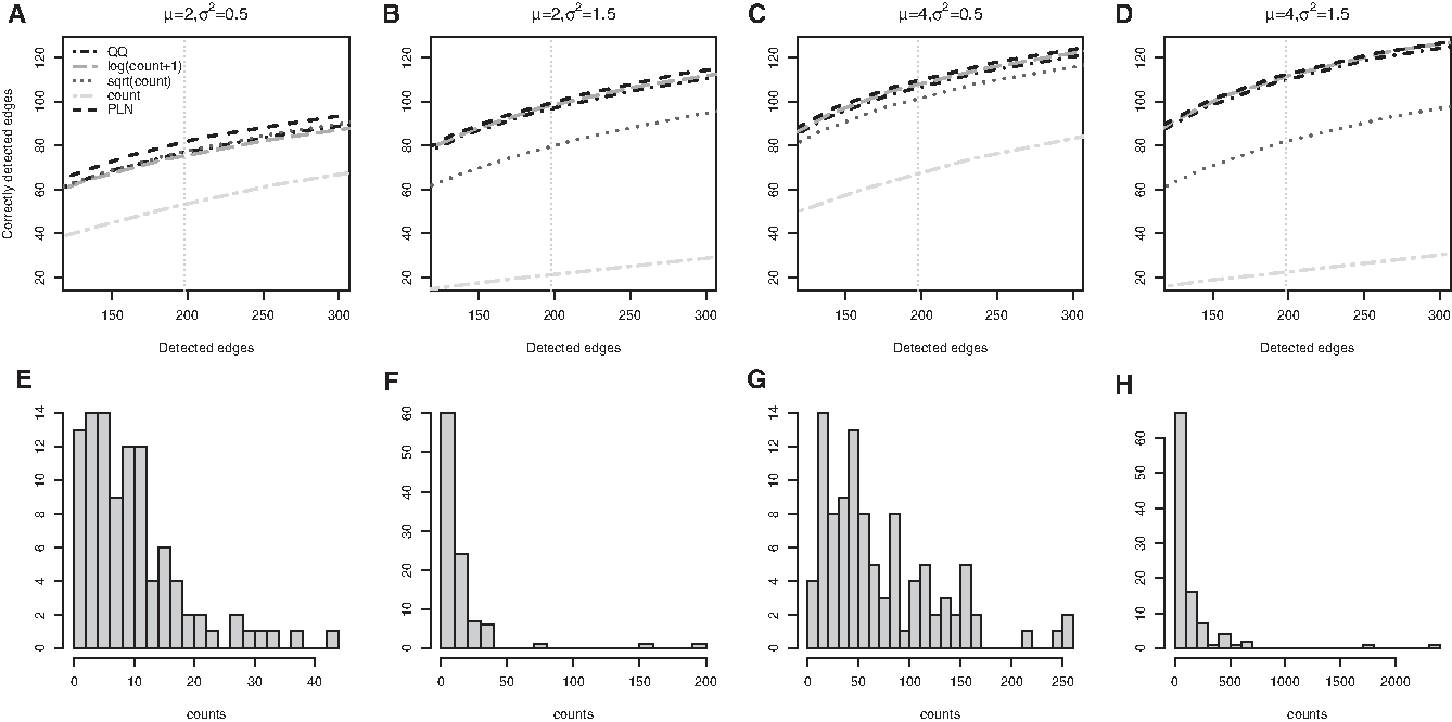
Power-net simulation 2. (A–D) The number of total detected edges (x-axis) and the number of correctly detected edges (y-axis) when \documentclass{aastex}\usepackage{amsbsy}\usepackage{amsfonts}\usepackage{amssymb}\usepackage{bm}\usepackage{mathrsfs}\usepackage{pifont}\usepackage{stmaryrd}\usepackage{textcomp}\usepackage{portland, xspace}\usepackage{amsmath, amsxtra}\usepackage{upgreek}\pagestyle{empty}\DeclareMathSizes{10}{9}{7}{6}\begin{document} $$( { \mu _j} , { \Sigma _{jj}} )$$ \end{document} are fixed at \documentclass{aastex}\usepackage{amsbsy}\usepackage{amsfonts}\usepackage{amssymb}\usepackage{bm}\usepackage{mathrsfs}\usepackage{pifont}\usepackage{stmaryrd}\usepackage{textcomp}\usepackage{portland, xspace}\usepackage{amsmath, amsxtra}\usepackage{upgreek}\pagestyle{empty}\DeclareMathSizes{10}{9}{7}{6}\begin{document} $$( 2 , 0.5 )$$ \end{document} , \documentclass{aastex}\usepackage{amsbsy}\usepackage{amsfonts}\usepackage{amssymb}\usepackage{bm}\usepackage{mathrsfs}\usepackage{pifont}\usepackage{stmaryrd}\usepackage{textcomp}\usepackage{portland, xspace}\usepackage{amsmath, amsxtra}\usepackage{upgreek}\pagestyle{empty}\DeclareMathSizes{10}{9}{7}{6}\begin{document} $$( 2 , 1.5 )$$ \end{document} , \documentclass{aastex}\usepackage{amsbsy}\usepackage{amsfonts}\usepackage{amssymb}\usepackage{bm}\usepackage{mathrsfs}\usepackage{pifont}\usepackage{stmaryrd}\usepackage{textcomp}\usepackage{portland, xspace}\usepackage{amsmath, amsxtra}\usepackage{upgreek}\pagestyle{empty}\DeclareMathSizes{10}{9}{7}{6}\begin{document} $$( 4 , 0.5 )$$ \end{document} , and \documentclass{aastex}\usepackage{amsbsy}\usepackage{amsfonts}\usepackage{amssymb}\usepackage{bm}\usepackage{mathrsfs}\usepackage{pifont}\usepackage{stmaryrd}\usepackage{textcomp}\usepackage{portland, xspace}\usepackage{amsmath, amsxtra}\usepackage{upgreek}\pagestyle{empty}\DeclareMathSizes{10}{9}{7}{6}\begin{document} $$( 4 , 1.5 )$$ \end{document} respectively. (E–H) Histograms of Poisson log-normal (PLN) counts when \documentclass{aastex}\usepackage{amsbsy}\usepackage{amsfonts}\usepackage{amssymb}\usepackage{bm}\usepackage{mathrsfs}\usepackage{pifont}\usepackage{stmaryrd}\usepackage{textcomp}\usepackage{portland, xspace}\usepackage{amsmath, amsxtra}\usepackage{upgreek}\pagestyle{empty}\DeclareMathSizes{10}{9}{7}{6}\begin{document} $$( { \mu _j} , { \Sigma _{jj}} )$$ \end{document} are fixed at \documentclass{aastex}\usepackage{amsbsy}\usepackage{amsfonts}\usepackage{amssymb}\usepackage{bm}\usepackage{mathrsfs}\usepackage{pifont}\usepackage{stmaryrd}\usepackage{textcomp}\usepackage{portland, xspace}\usepackage{amsmath, amsxtra}\usepackage{upgreek}\pagestyle{empty}\DeclareMathSizes{10}{9}{7}{6}\begin{document} $$( 2 , 0.5 )$$ \end{document} , \documentclass{aastex}\usepackage{amsbsy}\usepackage{amsfonts}\usepackage{amssymb}\usepackage{bm}\usepackage{mathrsfs}\usepackage{pifont}\usepackage{stmaryrd}\usepackage{textcomp}\usepackage{portland, xspace}\usepackage{amsmath, amsxtra}\usepackage{upgreek}\pagestyle{empty}\DeclareMathSizes{10}{9}{7}{6}\begin{document} $$( 2 , 1.5 )$$ \end{document} , \documentclass{aastex}\usepackage{amsbsy}\usepackage{amsfonts}\usepackage{amssymb}\usepackage{bm}\usepackage{mathrsfs}\usepackage{pifont}\usepackage{stmaryrd}\usepackage{textcomp}\usepackage{portland, xspace}\usepackage{amsmath, amsxtra}\usepackage{upgreek}\pagestyle{empty}\DeclareMathSizes{10}{9}{7}{6}\begin{document} $$( 4 , 0.5 )$$ \end{document} , and \documentclass{aastex}\usepackage{amsbsy}\usepackage{amsfonts}\usepackage{amssymb}\usepackage{bm}\usepackage{mathrsfs}\usepackage{pifont}\usepackage{stmaryrd}\usepackage{textcomp}\usepackage{portland, xspace}\usepackage{amsmath, amsxtra}\usepackage{upgreek}\pagestyle{empty}\DeclareMathSizes{10}{9}{7}{6}\begin{document} $$( 4 , 1.5 )$$ \end{document} , respectively.

With varying sample sizes of \documentclass{aastex}\usepackage{amsbsy}\usepackage{amsfonts}\usepackage{amssymb}\usepackage{bm}\usepackage{mathrsfs}\usepackage{pifont}\usepackage{stmaryrd}\usepackage{textcomp}\usepackage{portland, xspace}\usepackage{amsmath, amsxtra}\usepackage{upgreek}\pagestyle{empty}\DeclareMathSizes{10}{9}{7}{6}\begin{document} $$n = 50$$ \end{document} and \documentclass{aastex}\usepackage{amsbsy}\usepackage{amsfonts}\usepackage{amssymb}\usepackage{bm}\usepackage{mathrsfs}\usepackage{pifont}\usepackage{stmaryrd}\usepackage{textcomp}\usepackage{portland, xspace}\usepackage{amsmath, amsxtra}\usepackage{upgreek}\pagestyle{empty}\DeclareMathSizes{10}{9}{7}{6}\begin{document} $$n = 200$$ \end{document} , not surprisingly, the performance of all methods improves with increased sample size. At a smaller sample size, PLN has more prominent advantage in detecting correct edges, whereas at a larger sample size, PLN produces comparatively more accurate estimates of partial correlations (Supplementary Fig. S1).

It has been previously observed that gene expression in a cell follows a hierarchical structure, in which the expression levels of a few genes influence the expression levels of many other genes (Morley et al., 2004). In a graph, such a “master regulator” that appears as a hub, a node is connected with many other nodes. There is an increasing interest in identifying master regulators as they play central roles in gene regulation. To investigate the ability of detecting such hub nodes, we examine the edge-detection performance in two subnetworks of the power-law network. The underlying graphs are shown in Figure 4A and B: in one subnetwork, any node is connected to at most 12 other nodes (degree \documentclass{aastex}\usepackage{amsbsy}\usepackage{amsfonts}\usepackage{amssymb}\usepackage{bm}\usepackage{mathrsfs}\usepackage{pifont}\usepackage{stmaryrd}\usepackage{textcomp}\usepackage{portland, xspace}\usepackage{amsmath, amsxtra}\usepackage{upgreek}\pagestyle{empty}\DeclareMathSizes{10}{9}{7}{6}\begin{document} $$\le 12$$ \end{document} ) and there is no prominent hub; in contrast, the second subnetwork features a hub node of degree 28. Figure 4C and D compares the performance of these methods for the two subnetworks separately. Although PLN and graphical lasso with logarithm and quantile transformations perform similarly on the first subnetwork, the advantage of PLN in edge detection is more prominent in the presence of a hub node in the second subnetwork.

OPEN IN VIEWER

FIG. 4.

Power-net simulation 4: The performance on two subnetworks of the power-law network. \documentclass{aastex}\usepackage{amsbsy}\usepackage{amsfonts}\usepackage{amssymb}\usepackage{bm}\usepackage{mathrsfs}\usepackage{pifont}\usepackage{stmaryrd}\usepackage{textcomp}\usepackage{portland, xspace}\usepackage{amsmath, amsxtra}\usepackage{upgreek}\pagestyle{empty}\DeclareMathSizes{10}{9}{7}{6}\begin{document} $$( { \mu _j} , { \Sigma _{jj}} )$$ \end{document} are fixed at \documentclass{aastex}\usepackage{amsbsy}\usepackage{amsfonts}\usepackage{amssymb}\usepackage{bm}\usepackage{mathrsfs}\usepackage{pifont}\usepackage{stmaryrd}\usepackage{textcomp}\usepackage{portland, xspace}\usepackage{amsmath, amsxtra}\usepackage{upgreek}\pagestyle{empty}\DeclareMathSizes{10}{9}{7}{6}\begin{document} $$( 2 , 1 )$$ \end{document} ; methods are applied to the two subnetworks ( \documentclass{aastex}\usepackage{amsbsy}\usepackage{amsfonts}\usepackage{amssymb}\usepackage{bm}\usepackage{mathrsfs}\usepackage{pifont}\usepackage{stmaryrd}\usepackage{textcomp}\usepackage{portland, xspace}\usepackage{amsmath, amsxtra}\usepackage{upgreek}\pagestyle{empty}\DeclareMathSizes{10}{9}{7}{6}\begin{document} $$d = 100$$ \end{document} each) separately. (A) Subnetwork 1 has no prominent hub. (B) Subnetwork 2 has 1 hub gene with 28 edges. (C, D) The number of total detected edges (x-axis) and the number of correctly detected edges (y-axis) for subnetwork 1 and subnetwork 2, respectively.

We next perform simulation according to a network that we have previously constructed in a high-throughput proteomics study, varying signal strength in terms of magnitudes of the partial correlations (Wu et al., 2013). Again, all methods, except for applying graphical lasso to raw counts, perform competitively; the advantage of PLN becomes more apparent when the signals are weak (Supplementary Fig. S2C, F).

3.2. Application to RNA-seq data

Figure 5 and Supplementary Figure S3 display the inferred networks on the Geuvadis data using four different methods: PLN, neighborhood selection (MB), space, and graphical lasso; except for PLN, all other methods are applied to quantile-transformed data. All methods are tuned such that the number of detected edges is the same: 207 for EUR and 97 for YRI. We observe that the network inferred by PLN tends to be more concentrated and hub like; in other words, fewer genes are connected by at least one edge, but these connected genes tend to have higher degrees than those in the networks constructed by other methods. In EUR, modularities are \documentclass{aastex}\usepackage{amsbsy}\usepackage{amsfonts}\usepackage{amssymb}\usepackage{bm}\usepackage{mathrsfs}\usepackage{pifont}\usepackage{stmaryrd}\usepackage{textcomp}\usepackage{portland, xspace}\usepackage{amsmath, amsxtra}\usepackage{upgreek}\pagestyle{empty}\DeclareMathSizes{10}{9}{7}{6}\begin{document} $$0.32$$ \end{document} , \documentclass{aastex}\usepackage{amsbsy}\usepackage{amsfonts}\usepackage{amssymb}\usepackage{bm}\usepackage{mathrsfs}\usepackage{pifont}\usepackage{stmaryrd}\usepackage{textcomp}\usepackage{portland, xspace}\usepackage{amsmath, amsxtra}\usepackage{upgreek}\pagestyle{empty}\DeclareMathSizes{10}{9}{7}{6}\begin{document} $$0.36$$ \end{document} , \documentclass{aastex}\usepackage{amsbsy}\usepackage{amsfonts}\usepackage{amssymb}\usepackage{bm}\usepackage{mathrsfs}\usepackage{pifont}\usepackage{stmaryrd}\usepackage{textcomp}\usepackage{portland, xspace}\usepackage{amsmath, amsxtra}\usepackage{upgreek}\pagestyle{empty}\DeclareMathSizes{10}{9}{7}{6}\begin{document} $$0.37$$ \end{document} , and \documentclass{aastex}\usepackage{amsbsy}\usepackage{amsfonts}\usepackage{amssymb}\usepackage{bm}\usepackage{mathrsfs}\usepackage{pifont}\usepackage{stmaryrd}\usepackage{textcomp}\usepackage{portland, xspace}\usepackage{amsmath, amsxtra}\usepackage{upgreek}\pagestyle{empty}\DeclareMathSizes{10}{9}{7}{6}\begin{document} $$0.43$$ \end{document} for MB, space, graphical lasso, and PLN, respectively. In YRI, the corresponding modularities are \documentclass{aastex}\usepackage{amsbsy}\usepackage{amsfonts}\usepackage{amssymb}\usepackage{bm}\usepackage{mathrsfs}\usepackage{pifont}\usepackage{stmaryrd}\usepackage{textcomp}\usepackage{portland, xspace}\usepackage{amsmath, amsxtra}\usepackage{upgreek}\pagestyle{empty}\DeclareMathSizes{10}{9}{7}{6}\begin{document} $$0.37$$ \end{document} , \documentclass{aastex}\usepackage{amsbsy}\usepackage{amsfonts}\usepackage{amssymb}\usepackage{bm}\usepackage{mathrsfs}\usepackage{pifont}\usepackage{stmaryrd}\usepackage{textcomp}\usepackage{portland, xspace}\usepackage{amsmath, amsxtra}\usepackage{upgreek}\pagestyle{empty}\DeclareMathSizes{10}{9}{7}{6}\begin{document} $$0.50$$ \end{document} , \documentclass{aastex}\usepackage{amsbsy}\usepackage{amsfonts}\usepackage{amssymb}\usepackage{bm}\usepackage{mathrsfs}\usepackage{pifont}\usepackage{stmaryrd}\usepackage{textcomp}\usepackage{portland, xspace}\usepackage{amsmath, amsxtra}\usepackage{upgreek}\pagestyle{empty}\DeclareMathSizes{10}{9}{7}{6}\begin{document} $$0.57$$ \end{document} , and \documentclass{aastex}\usepackage{amsbsy}\usepackage{amsfonts}\usepackage{amssymb}\usepackage{bm}\usepackage{mathrsfs}\usepackage{pifont}\usepackage{stmaryrd}\usepackage{textcomp}\usepackage{portland, xspace}\usepackage{amsmath, amsxtra}\usepackage{upgreek}\pagestyle{empty}\DeclareMathSizes{10}{9}{7}{6}\begin{document} $$0.57$$ \end{document} for these four methods. We emphasize that the knowledge of functional annotation is not used in constructing the network. Therefore, the enrichment of edges connecting genes in the same GO category provides independent support that these networks recapitulate some degree of functional organization. Using this measure, the proposed PLN performs favorably compared with GGMs. Connected genes that do not fall in the same GO category may implicate uncharacterized gene function or incomplete pathways, thus offering candidates for future investigation. Moreover, we further compared hub genes between EUR and YRI networks inferred by PLN. Among top 10 high-degree genes, there were three genes (HSPA5, MANF, and PPIB) that are in common and two of them (HSPA5 and PPIB) belong to GO category; “protein transport, modification, and folding” also appear as high-degree genes in the protein network (Wu et al., 2013).

OPEN IN VIEWER

FIG. 5.

Application: The inferred networks on European population \documentclass{aastex}\usepackage{amsbsy}\usepackage{amsfonts}\usepackage{amssymb}\usepackage{bm}\usepackage{mathrsfs}\usepackage{pifont}\usepackage{stmaryrd}\usepackage{textcomp}\usepackage{portland, xspace}\usepackage{amsmath, amsxtra}\usepackage{upgreek}\pagestyle{empty}\DeclareMathSizes{10}{9}{7}{6}\begin{document} $$( n = 373 )$$ \end{document} . An edge is a solid line according to the gene ontology (GO) category if the two connecting nodes belong to the same category; otherwise, the edge is a dashed line. The number of detected edges is 207 for the PLN model and is matched to be the same for the three Gaussian graphical models (MB, space, and glasso).