Two-Exponential Models of Gene Expression Patterns for Noisy Experimental Data

Abstract

Spatial pattern formation of the primary anterior–posterior morphogenetic gradient of the transcription factor Bicoid (Bcd) has been studied experimentally and computationally for many years. Bcd specifies positional information for the downstream segmentation genes, affecting the fly body plan. More recently, a number of researchers have focused on the patterning dynamics of the underlying bcd messenger RNA (mRNA) gradient, which is translated into Bcd protein. New, more accurate techniques for visualizing bcd mRNA need to be combined with quantitative signal extraction techniques to reconstruct the bcd mRNA distribution. Here, we present a robust technique for quantifying gradients with a two-exponential model. This approach (1) has natural, biologically relevant parameters and (2) is invariant to linear transformations of the data arising due to variation in experimental conditions (e.g., microscope settings, nonspecific background signal). This allows us to quantify bcd mRNA gradient variability from embryo to embryo (important for studying the robustness of developmental regulatory networks); sort out atypical gradients; and classify embryos to developmental stage by quantitative gradient parameters.

1. Introduction

1.1. Biology

A key concept in developmental biology is that of morphogen gradients (Briscoe et al., 2010), in which a spatially distributed gradient of a signaling molecule (morphogen) affects downstream cellular responses in a concentration-dependent manner. These spatial gradients are established by molecular transport, either active or diffusional. One of the best-studied morphogen gradients in development is of the protein transcription factor Bicoid (Bcd; Briscoe et al., 2010; Grimm et al., 2010), which regulates gene expression along the anterior–posterior (AP) axis of the developing fruit fly (Drosophila) embryo. The Bcd protein gradient has been studied quantitatively for many years, both in terms of quantitative experiments and in mathematical modeling of the dynamics of gradient formation.

More recently, studies have focused on the underlying dynamics and patterning of the bcd messenger RNA (mRNA) gradient, since the Bcd protein forms via translation from the mRNA. The bcd RNA gradient forms earlier than the protein gradient and exhibits a number of distinct features from the protein pattern. These have been the subject of several mathematical modeling projects, as well as new quantitative experimental projects, to characterize the bcd mRNA gradient (Spirov et al., 2009; Lipshitz, 2009; Kavousanakis et al., 2010; Deng et al., 2010; Little et al., 2011; Cheung et al., 2011; Dalessi et al., 2012; Liu and Niranjan, 2012; Fahmy et al., 2014; Ali-Murthy and Kornberg, 2016).

There are a number of features to bcd RNA patterning making it more complex to study than the Bcd protein pattern. These features require new and more sophisticated techniques in data acquisition and signal processing to extract quantitative data. This article presents and validates a new method for quantitative analysis of spatial profiles of bcd RNA reliably extracted from whole-embryo three-dimensional (3D) scans (confocal microscopy) of fluorescent in situ hybridization (FISH) RNA data.

1.2. Data

Figure 1A shows a sagittal section through the middle of such a whole-embryo scan, with fluorescence intensity proportional to the concentration of bcd mRNA. The data set is 3D, and the RNA transport setting up this 3D pattern has components in the three coordinates: head-to-tail (AP); top-to-bottom (dorsoventral, DV); and inside-to-outside (basal–apical, BA). The gradient is chiefly along the AP direction: biologically, the mRNA spreads posteriorly from a maternal deposition at the anterior end of the embryo. There are, however, concentration differences in the DV direction, and while bcd RNA and protein patterns are most intense in the surface, or cortex, of the embryo, bcd is also found in the interior of the embryo, and there is a concentration gradient in the BA direction. The transport processes establishing these gradients may differ between the different coordinates: AP transport of bcd RNA involves minus-end motors trafficking along microtubules, assisted by proteins such as Staufen (Stau; Weil et al., 2006, 2008; Spirov et al., 2009; Fahmy et al., 2014; Ali-Murthy and Kornberg, 2016); DV “bending” of bcd pattern may reflect geometric asymmetries in the embryo; and BA transport appears to occur at later stages of development, by an unknown mechanism (Bullock and Ish-Horowicz, 2001; Spirov et al., 2009; Fahmy et al., 2014).

FIG. 1.

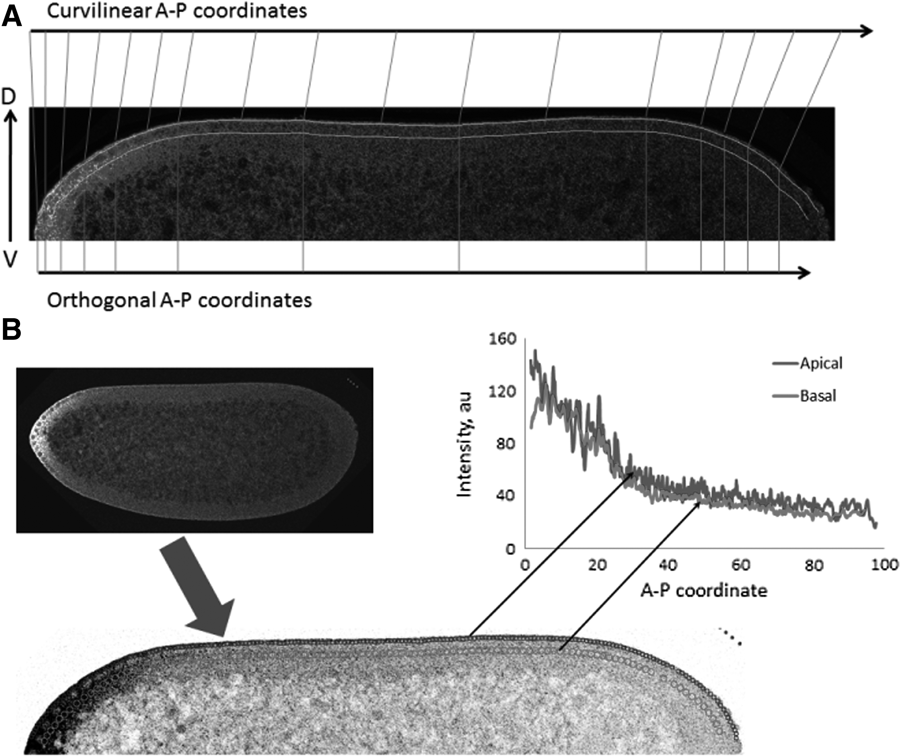
Preparation of data for quantitative analysis of sagittal images by 1D SSA. (A) Fluorescence intensity is proportional to the concentration of bcd RNA. The gradient in bcd mRNA is chiefly in the head-to-tail, AP, direction (left to right), but DV variation (top-to-bottom coordinate) can be seen, as well as variation by depth in the embryo (BA direction). For transport and patterning along the surface of the embryo, the natural coordinates are curvilinear. For extraction of the head-to-tail gradient patterning, the curvilinear coordinates are well approximated by a projection onto the AP axis (see Supplementary Material). (B) For quantification of the AP gradient and BA differences, we sample data from an apical layer above the cortical nuclei and from a basal layer below the cortical nuclei, using chains of overlapping ROIs. Data from each layer are analyzed independently with 1D SSA. Each layer can then be plotted as intensity versus AP position (right inset). 1D, one-dimensional; AP, anterior–posterior; BA, basal–apical; DV, dorsoventral; mRNA, messenger RNA; ROI, regions of interest; SSA, singular spectrum analysis.

1.3. Approach

In whole-embryo imaging, variability can arise during tissue fixation and staining with fluorophores, as well as from differences in microscope settings (gain and offset) between measurements of different batches of embryos on different days. Here, we discuss features of the data extraction that are insensitive to such experimental variation.

The aim of our approach is to create a model for apical and basal profiles (see Fig. 1B) with bcd gradients, estimate the model parameters, and show that they can help to obtain biological results, in particular, to compare different ages in the embryo development. We show an example of how data extracted and modeled by this technique can provide new biological insights into bcd RNA gradient formation.

The novelty of the approach consists in consideration of the model parameters, which do not depend on linear transformation of the data and thereby on the nonspecific background signal and the microscope settings. It is very important, since otherwise the comparison results can be caused by the experimental conditions, not by the biology reasons.

1.4. Model

A two-exponential fit of a Bcd protein profile can be well approximated by a single exponential plus a nearly constant background (Houchmandzadeh et al., 2002; Alexandrov et al., 2008). In contrast, while some bcd RNA profiles show such characteristics, many others, especially at early stages, show a much sharper exponential drop in the anterior, plus a constant or even posteriorly rising component through the rest of the embryo (Fig. 2). The transition between components can be readily visible in RNA patterns (and not in protein), as a “kink” around the 20% egg length (%EL)–30%EL position. These different components suggest multiple scales (or mechanisms) in the posterior-ward transport of bcd RNA.

FIG. 2.

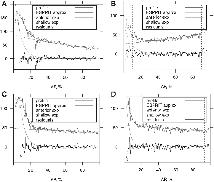
Representative examples of AP profiles of bcd mRNA, illustrating the variety of cases and efficacy of the modeling approach. The raw data are noisy; the smooth pattern is the ESPRIT fit, which is the sum of two exponentials; they are depicted individually: anterior exponential 1, which decreases to zero from the left; trunk shallow exponential 2, which is similar to a straight line. The residual noise is oscillating around zero. (A) An early nuclear cleavage cycle 14A (nc14) embryo with a typical broad anterior exponential and shallow second component extending throughout the embryo [Cf. Spirov et al. (2009)]. (B) A bcd mRNA profile in which the second, trunk, component rises toward the posterior (i.e., has a positive exponential rate). (C) A case with a nearly flat second component (representing the mRNA signal posterior of 25%EL). (D) An embryo with a very sharp anterior (first component) exponential, dropping to low values by 10%EL.

1.5. Technique

We previously applied a signal extraction technique based on singular spectrum analysis (SSA) to quantify Bcd protein gradients (Alexandrov et al., 2008). This demonstrated that SSA could reliably and automatically extract AP Bcd protein gradients. These were the sum of two exponentials, one with a significant decay constant (strong curvature) and one of nearly linear form, capturing the nonspecific background signal. Here, we adapt the SSA technique to the more complex cases of bcd RNA gradients, validating the reliability and effectiveness of the approach. SSA itself is used for signal extraction, and the SSA-related method ESPRIT (Roy and Kailath, 1989; Golyandina and Zhigljavsky, 2013) is used for the estimation of signal parameters.

SSA techniques have proven to be robust to signal extraction from data with substantial experimental variability and intrinsic noise (Golyandina et al., 2001; Alexandrov et al., 2008; Alonso et al., 2005; Golyandina et al., 2012; Golyandina and Zhigljavsky, 2013). The use of SSA for extraction of signals in gene expression data was in Spirov et al. (2012), Golyandina et al. (2012), and Shlemov et al. (2015a,b).

2. Methods

2.1. Two-exponential modeling

2.1.1. Description of the model

We fit the following two-exponential function (of AP distance, x) to bcd mRNA data, to capture the distinct two-component pattern of most bcd RNA gradients (with the “kink,” commonly observed at 20%EL–30%EL): \documentclass{aastex}\usepackage{amsbsy}\usepackage{amsfonts}\usepackage{amssymb}\usepackage{bm}\usepackage{mathrsfs}\usepackage{pifont}\usepackage{stmaryrd}\usepackage{textcomp}\usepackage{portland, xspace}\usepackage{amsmath, amsxtra}\usepackage{upgreek}\pagestyle{empty}\DeclareMathSizes{10}{9}{7}{6}\begin{document} \begin{align*} s ( x ) = {C_1} \exp ( { \alpha _1}x ) + {C_2} \exp ( { \alpha _2}x ) , \tag{1} \end{align*} \end{document}

or \documentclass{aastex}\usepackage{amsbsy}\usepackage{amsfonts}\usepackage{amssymb}\usepackage{bm}\usepackage{mathrsfs}\usepackage{pifont}\usepackage{stmaryrd}\usepackage{textcomp}\usepackage{portland, xspace}\usepackage{amsmath, amsxtra}\usepackage{upgreek}\pagestyle{empty}\DeclareMathSizes{10}{9}{7}{6}\begin{document} \begin{align*} s ( x ) = {C_1} \lambda _1^x + {C_2} \lambda _2^x , \end{align*} \end{document}

for \documentclass{aastex}\usepackage{amsbsy}\usepackage{amsfonts}\usepackage{amssymb}\usepackage{bm}\usepackage{mathrsfs}\usepackage{pifont}\usepackage{stmaryrd}\usepackage{textcomp}\usepackage{portland, xspace}\usepackage{amsmath, amsxtra}\usepackage{upgreek}\pagestyle{empty}\DeclareMathSizes{10}{9}{7}{6}\begin{document} $${ \lambda _i} = e_i^ \alpha$$ \end{document} . The two components, where the first we call anterior (for the sharp, quickly decaying pattern in the anterior) and the second we call shallow (for the more constant component in the mid- and posterior embryo), each have two parameters—an amplitude C and a rate \documentclass{aastex}\usepackage{amsbsy}\usepackage{amsfonts}\usepackage{amssymb}\usepackage{bm}\usepackage{mathrsfs}\usepackage{pifont}\usepackage{stmaryrd}\usepackage{textcomp}\usepackage{portland, xspace}\usepackage{amsmath, amsxtra}\usepackage{upgreek}\pagestyle{empty}\DeclareMathSizes{10}{9}{7}{6}\begin{document} $$\alpha$$ \end{document} (or an exponential base \documentclass{aastex}\usepackage{amsbsy}\usepackage{amsfonts}\usepackage{amssymb}\usepackage{bm}\usepackage{mathrsfs}\usepackage{pifont}\usepackage{stmaryrd}\usepackage{textcomp}\usepackage{portland, xspace}\usepackage{amsmath, amsxtra}\usepackage{upgreek}\pagestyle{empty}\DeclareMathSizes{10}{9}{7}{6}\begin{document} $$\lambda$$ \end{document} ). In biological terms, C in \documentclass{aastex}\usepackage{amsbsy}\usepackage{amsfonts}\usepackage{amssymb}\usepackage{bm}\usepackage{mathrsfs}\usepackage{pifont}\usepackage{stmaryrd}\usepackage{textcomp}\usepackage{portland, xspace}\usepackage{amsmath, amsxtra}\usepackage{upgreek}\pagestyle{empty}\DeclareMathSizes{10}{9}{7}{6}\begin{document} $$C{ \lambda ^x}$$ \end{document} for \documentclass{aastex}\usepackage{amsbsy}\usepackage{amsfonts}\usepackage{amssymb}\usepackage{bm}\usepackage{mathrsfs}\usepackage{pifont}\usepackage{stmaryrd}\usepackage{textcomp}\usepackage{portland, xspace}\usepackage{amsmath, amsxtra}\usepackage{upgreek}\pagestyle{empty}\DeclareMathSizes{10}{9}{7}{6}\begin{document} $$\lambda < 1$$ \end{document} represents the maximum concentration of the exponential component, and \documentclass{aastex}\usepackage{amsbsy}\usepackage{amsfonts}\usepackage{amssymb}\usepackage{bm}\usepackage{mathrsfs}\usepackage{pifont}\usepackage{stmaryrd}\usepackage{textcomp}\usepackage{portland, xspace}\usepackage{amsmath, amsxtra}\usepackage{upgreek}\pagestyle{empty}\DeclareMathSizes{10}{9}{7}{6}\begin{document} $$\alpha$$ \end{document} (and therefore \documentclass{aastex}\usepackage{amsbsy}\usepackage{amsfonts}\usepackage{amssymb}\usepackage{bm}\usepackage{mathrsfs}\usepackage{pifont}\usepackage{stmaryrd}\usepackage{textcomp}\usepackage{portland, xspace}\usepackage{amsmath, amsxtra}\usepackage{upgreek}\pagestyle{empty}\DeclareMathSizes{10}{9}{7}{6}\begin{document} $$\lambda$$ \end{document} ) represents the rate at which the component decreases (or increases) along the AP coordinate. The anterior exponential is always decreasing and therefore \documentclass{aastex}\usepackage{amsbsy}\usepackage{amsfonts}\usepackage{amssymb}\usepackage{bm}\usepackage{mathrsfs}\usepackage{pifont}\usepackage{stmaryrd}\usepackage{textcomp}\usepackage{portland, xspace}\usepackage{amsmath, amsxtra}\usepackage{upgreek}\pagestyle{empty}\DeclareMathSizes{10}{9}{7}{6}\begin{document} $${ \lambda _1} < 1$$ \end{document} , \documentclass{aastex}\usepackage{amsbsy}\usepackage{amsfonts}\usepackage{amssymb}\usepackage{bm}\usepackage{mathrsfs}\usepackage{pifont}\usepackage{stmaryrd}\usepackage{textcomp}\usepackage{portland, xspace}\usepackage{amsmath, amsxtra}\usepackage{upgreek}\pagestyle{empty}\DeclareMathSizes{10}{9}{7}{6}\begin{document} $${ \alpha _1} < 0$$ \end{document} ; while the shallow exponential can be decreasing or increasing (Fig. 2).

One-exponential plus constant background is a special case of Equation (1), with the rate \documentclass{aastex}\usepackage{amsbsy}\usepackage{amsfonts}\usepackage{amssymb}\usepackage{bm}\usepackage{mathrsfs}\usepackage{pifont}\usepackage{stmaryrd}\usepackage{textcomp}\usepackage{portland, xspace}\usepackage{amsmath, amsxtra}\usepackage{upgreek}\pagestyle{empty}\DeclareMathSizes{10}{9}{7}{6}\begin{document} $${ \alpha _2} = 0$$ \end{document} (the base \documentclass{aastex}\usepackage{amsbsy}\usepackage{amsfonts}\usepackage{amssymb}\usepackage{bm}\usepackage{mathrsfs}\usepackage{pifont}\usepackage{stmaryrd}\usepackage{textcomp}\usepackage{portland, xspace}\usepackage{amsmath, amsxtra}\usepackage{upgreek}\pagestyle{empty}\DeclareMathSizes{10}{9}{7}{6}\begin{document} $${ \lambda _2} = 1$$ \end{document} ). Use of Equation (1) does not require two strong (nonzero \documentclass{aastex}\usepackage{amsbsy}\usepackage{amsfonts}\usepackage{amssymb}\usepackage{bm}\usepackage{mathrsfs}\usepackage{pifont}\usepackage{stmaryrd}\usepackage{textcomp}\usepackage{portland, xspace}\usepackage{amsmath, amsxtra}\usepackage{upgreek}\pagestyle{empty}\DeclareMathSizes{10}{9}{7}{6}\begin{document} $$\alpha$$ \end{document} ) exponentials in the signal (pattern). In the case of the model commonly applied to the Bcd protein gradient, the first exponential describes the signal and the second exponential describes the nonspecific background signal and the offset of the microscope.

Note that raw image data are likely of the form \documentclass{aastex}\usepackage{amsbsy}\usepackage{amsfonts}\usepackage{amssymb}\usepackage{bm}\usepackage{mathrsfs}\usepackage{pifont}\usepackage{stmaryrd}\usepackage{textcomp}\usepackage{portland, xspace}\usepackage{amsmath, amsxtra}\usepackage{upgreek}\pagestyle{empty}\DeclareMathSizes{10}{9}{7}{6}\begin{document} $$s ( x ) + \varepsilon ( x )$$ \end{document} , where \documentclass{aastex}\usepackage{amsbsy}\usepackage{amsfonts}\usepackage{amssymb}\usepackage{bm}\usepackage{mathrsfs}\usepackage{pifont}\usepackage{stmaryrd}\usepackage{textcomp}\usepackage{portland, xspace}\usepackage{amsmath, amsxtra}\usepackage{upgreek}\pagestyle{empty}\DeclareMathSizes{10}{9}{7}{6}\begin{document} $$\varepsilon ( x )$$ \end{document} represents “noise,” that is, nonregular oscillations with zero mean.

2.1.2. Model characteristics independent of the microscopy gain/offset and background

To remove effects from variability in microscope settings (gain and offset) and the unknown form of nonspecific background (Houchmandzadeh et al., 2002; Myasnikova et al., 2005; Holloway et al., 2006), gradient characteristics can be used, which do not change under a linear transformation of the gradient.

That is, if each profile (gradient) can be represented by the linear transformation: \documentclass{aastex}\usepackage{amsbsy}\usepackage{amsfonts}\usepackage{amssymb}\usepackage{bm}\usepackage{mathrsfs}\usepackage{pifont}\usepackage{stmaryrd}\usepackage{textcomp}\usepackage{portland, xspace}\usepackage{amsmath, amsxtra}\usepackage{upgreek}\pagestyle{empty}\DeclareMathSizes{10}{9}{7}{6}\begin{document} \begin{align*} f ( x ) = A ( s ( x ) + \varepsilon ( x ) ) + B , \tag{2} \end{align*} \end{document}

where \documentclass{aastex}\usepackage{amsbsy}\usepackage{amsfonts}\usepackage{amssymb}\usepackage{bm}\usepackage{mathrsfs}\usepackage{pifont}\usepackage{stmaryrd}\usepackage{textcomp}\usepackage{portland, xspace}\usepackage{amsmath, amsxtra}\usepackage{upgreek}\pagestyle{empty}\DeclareMathSizes{10}{9}{7}{6}\begin{document} $$A > 0$$ \end{document} and B represent an unknown scaling and an unknown offset, respectively. A and B are likely to differ between embryos (with different staining conditions, microscope settings, etc.), but when we take apical and basal traces within each embryo image, we assume that the A and B are constant within a single embryo. To compare data between embryos, we take advantage of the independence of the profile characteristics from linear transformations, that is, independence from A and B values.

The signal given by Equation (1) has characteristics that approximately satisfy independency from linear transformations if the second (shallow gradient) exponential rate is small enough ( \documentclass{aastex}\usepackage{amsbsy}\usepackage{amsfonts}\usepackage{amssymb}\usepackage{bm}\usepackage{mathrsfs}\usepackage{pifont}\usepackage{stmaryrd}\usepackage{textcomp}\usepackage{portland, xspace}\usepackage{amsmath, amsxtra}\usepackage{upgreek}\pagestyle{empty}\DeclareMathSizes{10}{9}{7}{6}\begin{document} $$ { \alpha _2 } \mathbin { \approxeq } 0$$ \end{document} , \documentclass{aastex}\usepackage{amsbsy}\usepackage{amsfonts}\usepackage{amssymb}\usepackage{bm}\usepackage{mathrsfs}\usepackage{pifont}\usepackage{stmaryrd}\usepackage{textcomp}\usepackage{portland, xspace}\usepackage{amsmath, amsxtra}\usepackage{upgreek}\pagestyle{empty}\DeclareMathSizes{10}{9}{7}{6}\begin{document} $${ \lambda _2 } = { e^ { { \alpha _2 } }} \mathbin { \approxeq} 1$$ \end{document} ) and can therefore be approximated by a linear function. This is a reasonable assumption for the bcd mRNA data, giving \documentclass{aastex}\usepackage{amsbsy}\usepackage{amsfonts}\usepackage{amssymb}\usepackage{bm}\usepackage{mathrsfs}\usepackage{pifont}\usepackage{stmaryrd}\usepackage{textcomp}\usepackage{portland, xspace}\usepackage{amsmath, amsxtra}\usepackage{upgreek}\pagestyle{empty}\DeclareMathSizes{10}{9}{7}{6}\begin{document} \begin{align*} A ( {C_1} \exp ( { \alpha _1}x ) + {C_2} \exp ( { \alpha _2}x ) ) + B \approx \end{align*} \end{document} \documentclass{aastex}\usepackage{amsbsy}\usepackage{amsfonts}\usepackage{amssymb}\usepackage{bm}\usepackage{mathrsfs}\usepackage{pifont}\usepackage{stmaryrd}\usepackage{textcomp}\usepackage{portland, xspace}\usepackage{amsmath, amsxtra}\usepackage{upgreek}\pagestyle{empty}\DeclareMathSizes{10}{9}{7}{6}\begin{document} \begin{align*} A{C_1} \exp ( { \alpha _1}x ) + A{C_2} ( 1 + { \alpha _2}x ) + B \approx { \tilde C_1} \exp ( { \tilde \alpha _1}x ) + { \tilde C_2} \exp ( { \tilde \alpha _2}x ) , \end{align*} \end{document}

One can see that some parameters (e.g., the pre-exponential coefficients C₁ and C₂) depend on A and/or B, while the rate of the first exponential \documentclass{aastex}\usepackage{amsbsy}\usepackage{amsfonts}\usepackage{amssymb}\usepackage{bm}\usepackage{mathrsfs}\usepackage{pifont}\usepackage{stmaryrd}\usepackage{textcomp}\usepackage{portland, xspace}\usepackage{amsmath, amsxtra}\usepackage{upgreek}\pagestyle{empty}\DeclareMathSizes{10}{9}{7}{6}\begin{document} $${ \alpha _1}$$ \end{document} is not affected by linear transformations. In addition, we assume that the coefficients before the first and second exponentials are positive (true, generally, for the bcd RNA data) for \documentclass{aastex}\usepackage{amsbsy}\usepackage{amsfonts}\usepackage{amssymb}\usepackage{bm}\usepackage{mathrsfs}\usepackage{pifont}\usepackage{stmaryrd}\usepackage{textcomp}\usepackage{portland, xspace}\usepackage{amsmath, amsxtra}\usepackage{upgreek}\pagestyle{empty}\DeclareMathSizes{10}{9}{7}{6}\begin{document} $$A > 0$$ \end{document} and B, which appear in the experiments. Then, the sign of \documentclass{aastex}\usepackage{amsbsy}\usepackage{amsfonts}\usepackage{amssymb}\usepackage{bm}\usepackage{mathrsfs}\usepackage{pifont}\usepackage{stmaryrd}\usepackage{textcomp}\usepackage{portland, xspace}\usepackage{amsmath, amsxtra}\usepackage{upgreek}\pagestyle{empty}\DeclareMathSizes{10}{9}{7}{6}\begin{document} $${ \alpha _2}$$ \end{document} is also stable to the transformation and determines if the second (shallow) exponential either increases or decreases. The negative sign of C₁ or C₂ can be used for detection of profiles that do not fit the model.

Note that similar considerations about parameters independent on linear transformations can be applied to any number of active exponentials (e.g., we can consider both anterior and tail ones and study their rates), while the shallow exponential should be alone. It is important that the noise level directly depends on the scaling A and therefore we do not use it as an embryo characteristic.

2.1.3. Model characteristics of apical and basal profiles

We apply the model to both apical and basal profiles, adding corresponding upper indices to parameter notation. Several characteristics that reflect the relationship between two profiles of the same embryo (therefore, A and B are the same for both profiles) can be added. For clarity, we will write “anterior” or “shallow” in the lower indices instead of 1 and 2 correspondingly.

Thus, the following combinations of the model parameters of the profiles can be considered almost independent of a linear transformation of the intensities, that is, of A and B: \documentclass{aastex}\usepackage{amsbsy}\usepackage{amsfonts}\usepackage{amssymb}\usepackage{bm}\usepackage{mathrsfs}\usepackage{pifont}\usepackage{stmaryrd}\usepackage{textcomp}\usepackage{portland, xspace}\usepackage{amsmath, amsxtra}\usepackage{upgreek}\pagestyle{empty}\DeclareMathSizes{10}{9}{7}{6}\begin{document} \begin{align*} \alpha _{{ \rm{anterior}}}^{ ( { \rm{apical}} ) } , \quad \quad {\rm sign} ( \alpha _{{ \rm{shallow}}}^{ ( { \rm{apical}} ) } ) , \quad \quad C_{{ \rm{shallow}}}^{ ( { \rm{apical}} ) } \alpha _{{ \rm{shallow}}}^{ ( { \rm{apical}} ) } / C_{{ \rm{anterior}}}^{ ( { \rm{apical}} ) } , \tag{3} \end{align*} \end{document} \documentclass{aastex}\usepackage{amsbsy}\usepackage{amsfonts}\usepackage{amssymb}\usepackage{bm}\usepackage{mathrsfs}\usepackage{pifont}\usepackage{stmaryrd}\usepackage{textcomp}\usepackage{portland, xspace}\usepackage{amsmath, amsxtra}\usepackage{upgreek}\pagestyle{empty}\DeclareMathSizes{10}{9}{7}{6}\begin{document} \begin{align*} \alpha _{{ \rm{anterior}}}^{ ( { \rm{basal}} ) } , \quad \quad {\rm sign} ( \alpha _{{ \rm{shallow}}}^{ ( { \rm{basal}} ) } ) , \quad \quad C_{{ \rm{shallow}}}^{ ( { \rm{basal}} ) } \alpha _{{ \rm{shallow}}}^{ ( { \rm{basal}} ) } / C_{{ \rm{anterior}}}^{ ( { \rm{basal}} ) } , \tag{4} \end{align*} \end{document} \documentclass{aastex}\usepackage{amsbsy}\usepackage{amsfonts}\usepackage{amssymb}\usepackage{bm}\usepackage{mathrsfs}\usepackage{pifont}\usepackage{stmaryrd}\usepackage{textcomp}\usepackage{portland, xspace}\usepackage{amsmath, amsxtra}\usepackage{upgreek}\pagestyle{empty}\DeclareMathSizes{10}{9}{7}{6}\begin{document} \begin{align*} C_{{ \rm{anterior}}}^{ ( { \rm{apical}} ) } / C_{{ \rm{anterior}}}^{ ( { \rm{basal}} ) } , \quad \quad C_{{ \rm{shallow}}}^{ ( { \rm{apical}} ) } \alpha _{{ \rm{shallow}}}^{ ( { \rm{apical}} ) } / ( C_{{ \rm{shallow}}}^{ ( { \rm{basal}} ) } \alpha _{{ \rm{shallow}}}^{ ( { \rm{basal}} ) } ) , \tag{5} \end{align*} \end{document}

where Equation (3) are characteristics of apical profiles, Equation (4) are characteristics of basal profiles, and characteristics of Equation (5) show relationships between apical and basal profiles.

Hereinafter we use the following model characteristics based on these combinations:

the anterior gradient rates \documentclass{aastex}\usepackage{amsbsy}\usepackage{amsfonts}\usepackage{amssymb}\usepackage{bm}\usepackage{mathrsfs}\usepackage{pifont}\usepackage{stmaryrd}\usepackage{textcomp}\usepackage{portland, xspace}\usepackage{amsmath, amsxtra}\usepackage{upgreek}\pagestyle{empty}\DeclareMathSizes{10}{9}{7}{6}\begin{document} $$\lambda _{\rm{anterior}}^{ ( \rm{apical} ) } = \exp ( \alpha _{\rm{anterior}}^{ ( \rm{apical} ) })$$ \end{document} and \documentclass{aastex}\usepackage{amsbsy}\usepackage{amsfonts}\usepackage{amssymb}\usepackage{bm}\usepackage{mathrsfs}\usepackage{pifont}\usepackage{stmaryrd}\usepackage{textcomp}\usepackage{portland, xspace}\usepackage{amsmath, amsxtra}\usepackage{upgreek}\pagestyle{empty}\DeclareMathSizes{10}{9}{7}{6}\begin{document} $${ \rm{ \lambda }}_{{ \rm{anterior}}}^{ ( { \rm{basal}} ) } = \exp ( \alpha _{{ \rm{anterior}}}^{ ( { \rm{basal}} ) })\,;$$ \end{document}

the logarithmic ratio between the anterior gradient pre-exponential coefficients for the apical and basal profiles \documentclass{aastex}\usepackage{amsbsy}\usepackage{amsfonts}\usepackage{amssymb}\usepackage{bm}\usepackage{mathrsfs}\usepackage{pifont}\usepackage{stmaryrd}\usepackage{textcomp}\usepackage{portland, xspace}\usepackage{amsmath, amsxtra}\usepackage{upgreek}\pagestyle{empty}\DeclareMathSizes{10}{9}{7}{6}\begin{document} $${C^{{ \rm{ab}}}} = \ln ( C_{{ \rm{anterior}}}^{ ( { \rm{apical}} ) } / C_{{ \rm{anterior}}}^{ ( { \rm{basal}} ) } )$$ \end{document} ;

indicators of nonincrease in the shallow components \documentclass{aastex}\usepackage{amsbsy}\usepackage{amsfonts}\usepackage{amssymb}\usepackage{bm}\usepackage{mathrsfs}\usepackage{pifont}\usepackage{stmaryrd}\usepackage{textcomp}\usepackage{portland, xspace}\usepackage{amsmath, amsxtra}\usepackage{upgreek}\pagestyle{empty}\DeclareMathSizes{10}{9}{7}{6}\begin{document} $${ \rm{ \lambda }}_{{ \rm{shallow}}}^{ ( { \rm{apical}} ) } \le 1$$ \end{document} and \documentclass{aastex}\usepackage{amsbsy}\usepackage{amsfonts}\usepackage{amssymb}\usepackage{bm}\usepackage{mathrsfs}\usepackage{pifont}\usepackage{stmaryrd}\usepackage{textcomp}\usepackage{portland, xspace}\usepackage{amsmath, amsxtra}\usepackage{upgreek}\pagestyle{empty}\DeclareMathSizes{10}{9}{7}{6}\begin{document} $${ \rm{ \lambda }}_{{ \rm{shallow}}}^{{ \rm{ ( basal}} ) } \le 1$$ \end{document} .

Note that these characteristics have sense if \documentclass{aastex}\usepackage{amsbsy}\usepackage{amsfonts}\usepackage{amssymb}\usepackage{bm}\usepackage{mathrsfs}\usepackage{pifont}\usepackage{stmaryrd}\usepackage{textcomp}\usepackage{portland, xspace}\usepackage{amsmath, amsxtra}\usepackage{upgreek}\pagestyle{empty}\DeclareMathSizes{10}{9}{7}{6}\begin{document} $$C_{{ \rm{anterior}}}^{ ( { \rm{apical}} ) }$$ \end{document} , \documentclass{aastex}\usepackage{amsbsy}\usepackage{amsfonts}\usepackage{amssymb}\usepackage{bm}\usepackage{mathrsfs}\usepackage{pifont}\usepackage{stmaryrd}\usepackage{textcomp}\usepackage{portland, xspace}\usepackage{amsmath, amsxtra}\usepackage{upgreek}\pagestyle{empty}\DeclareMathSizes{10}{9}{7}{6}\begin{document} $$C_{{ \rm{anterior}}}^{ ( { \rm{basal}} ) }$$ \end{document} , \documentclass{aastex}\usepackage{amsbsy}\usepackage{amsfonts}\usepackage{amssymb}\usepackage{bm}\usepackage{mathrsfs}\usepackage{pifont}\usepackage{stmaryrd}\usepackage{textcomp}\usepackage{portland, xspace}\usepackage{amsmath, amsxtra}\usepackage{upgreek}\pagestyle{empty}\DeclareMathSizes{10}{9}{7}{6}\begin{document} $$C_{{ \rm{shallow}}}^{ ( { \rm{apical}} ) }$$ \end{document} , and \documentclass{aastex}\usepackage{amsbsy}\usepackage{amsfonts}\usepackage{amssymb}\usepackage{bm}\usepackage{mathrsfs}\usepackage{pifont}\usepackage{stmaryrd}\usepackage{textcomp}\usepackage{portland, xspace}\usepackage{amsmath, amsxtra}\usepackage{upgreek}\pagestyle{empty}\DeclareMathSizes{10}{9}{7}{6}\begin{document} $$C_{{ \rm{sallow}}}^{ ( { \rm{basal}} ) }$$ \end{document} are positive. Constructing the model, we assumed that the anterior exponential vanishes within the embryo length. To check it, let us consider additional characteristics: the AP positions \documentclass{aastex}\usepackage{amsbsy}\usepackage{amsfonts}\usepackage{amssymb}\usepackage{bm}\usepackage{mathrsfs}\usepackage{pifont}\usepackage{stmaryrd}\usepackage{textcomp}\usepackage{portland, xspace}\usepackage{amsmath, amsxtra}\usepackage{upgreek}\pagestyle{empty}\DeclareMathSizes{10}{9}{7}{6}\begin{document} $$AP0_{{ \rm{anterior}}}^{ ( { \rm{apical}} ) }$$ \end{document} and \documentclass{aastex}\usepackage{amsbsy}\usepackage{amsfonts}\usepackage{amssymb}\usepackage{bm}\usepackage{mathrsfs}\usepackage{pifont}\usepackage{stmaryrd}\usepackage{textcomp}\usepackage{portland, xspace}\usepackage{amsmath, amsxtra}\usepackage{upgreek}\pagestyle{empty}\DeclareMathSizes{10}{9}{7}{6}\begin{document} $$AP0_{{ \rm{anterior}}}^{ ( { \rm{basal}} ) }$$ \end{document} at which the anterior exponentials become almost zero (more precisely, such percent x %EL that \documentclass{aastex}\usepackage{amsbsy}\usepackage{amsfonts}\usepackage{amssymb}\usepackage{bm}\usepackage{mathrsfs}\usepackage{pifont}\usepackage{stmaryrd}\usepackage{textcomp}\usepackage{portland, xspace}\usepackage{amsmath, amsxtra}\usepackage{upgreek}\pagestyle{empty}\DeclareMathSizes{10}{9}{7}{6}\begin{document} $$C{ \lambda ^x} < 1$$ \end{document} ; recall that the intensity is measured in the range 0–255). These characteristics can be affected by a scaling and therefore should be used carefully.

These relationships underlie the quantitative conclusions in this article. We also use these relationships to screen for atypical embryos and outliers, aiding in following the development of the bcd RNA gradient over time and for studying apical–basal differences.

2.1.4. Estimation of the two-exponential model parameters

We use the subspace-based method ESPRIT, motivated by the success of SSA (also a subspace-based method) in smoothing one-dimensional (1D) gene profiles from Drosophila embryos (Alonso et al., 2005; Golyandina et al., 2012). On profiles from different genes, the method proved to be robust to high noise and to variations in embryo characteristics.

The mathematical details of ESPRIT can be found in Supplementary Material. We use the method to estimate the exponential decays in Equation (1): \documentclass{aastex}\usepackage{amsbsy}\usepackage{amsfonts}\usepackage{amssymb}\usepackage{bm}\usepackage{mathrsfs}\usepackage{pifont}\usepackage{stmaryrd}\usepackage{textcomp}\usepackage{portland, xspace}\usepackage{amsmath, amsxtra}\usepackage{upgreek}\pagestyle{empty}\DeclareMathSizes{10}{9}{7}{6}\begin{document} $${ \rm{ \lambda }}_{{ \rm{anterior}}}^{ ( { \rm{apical}} ) }$$ \end{document} , \documentclass{aastex}\usepackage{amsbsy}\usepackage{amsfonts}\usepackage{amssymb}\usepackage{bm}\usepackage{mathrsfs}\usepackage{pifont}\usepackage{stmaryrd}\usepackage{textcomp}\usepackage{portland, xspace}\usepackage{amsmath, amsxtra}\usepackage{upgreek}\pagestyle{empty}\DeclareMathSizes{10}{9}{7}{6}\begin{document} $${ \rm{ \lambda }}_{{ \rm{anterior}}}^{ ( { \rm{basal}} ) }$$ \end{document} , \documentclass{aastex}\usepackage{amsbsy}\usepackage{amsfonts}\usepackage{amssymb}\usepackage{bm}\usepackage{mathrsfs}\usepackage{pifont}\usepackage{stmaryrd}\usepackage{textcomp}\usepackage{portland, xspace}\usepackage{amsmath, amsxtra}\usepackage{upgreek}\pagestyle{empty}\DeclareMathSizes{10}{9}{7}{6}\begin{document} $${ \rm{ \lambda }}_{{ \rm{shallow}}}^{ ( { \rm{apical}} ) }$$ \end{document} , and \documentclass{aastex}\usepackage{amsbsy}\usepackage{amsfonts}\usepackage{amssymb}\usepackage{bm}\usepackage{mathrsfs}\usepackage{pifont}\usepackage{stmaryrd}\usepackage{textcomp}\usepackage{portland, xspace}\usepackage{amsmath, amsxtra}\usepackage{upgreek}\pagestyle{empty}\DeclareMathSizes{10}{9}{7}{6}\begin{document} $${ \rm{ \lambda }}_{{ \rm{shallow}}}^{ ( { \rm{basal}} ) }$$ \end{document} . The estimation of the coefficients \documentclass{aastex}\usepackage{amsbsy}\usepackage{amsfonts}\usepackage{amssymb}\usepackage{bm}\usepackage{mathrsfs}\usepackage{pifont}\usepackage{stmaryrd}\usepackage{textcomp}\usepackage{portland, xspace}\usepackage{amsmath, amsxtra}\usepackage{upgreek}\pagestyle{empty}\DeclareMathSizes{10}{9}{7}{6}\begin{document} $$C_{{ \rm{anterior}}}^{ ( { \rm{apical}} ) }$$ \end{document} , \documentclass{aastex}\usepackage{amsbsy}\usepackage{amsfonts}\usepackage{amssymb}\usepackage{bm}\usepackage{mathrsfs}\usepackage{pifont}\usepackage{stmaryrd}\usepackage{textcomp}\usepackage{portland, xspace}\usepackage{amsmath, amsxtra}\usepackage{upgreek}\pagestyle{empty}\DeclareMathSizes{10}{9}{7}{6}\begin{document} $$C_{{ \rm{anterior}}}^{ ( { \rm{basal}} ) }$$ \end{document} , \documentclass{aastex}\usepackage{amsbsy}\usepackage{amsfonts}\usepackage{amssymb}\usepackage{bm}\usepackage{mathrsfs}\usepackage{pifont}\usepackage{stmaryrd}\usepackage{textcomp}\usepackage{portland, xspace}\usepackage{amsmath, amsxtra}\usepackage{upgreek}\pagestyle{empty}\DeclareMathSizes{10}{9}{7}{6}\begin{document} $$C_{{ \rm{shallow}}}^{ ( { \rm{apical}} ) }$$ \end{document} , and \documentclass{aastex}\usepackage{amsbsy}\usepackage{amsfonts}\usepackage{amssymb}\usepackage{bm}\usepackage{mathrsfs}\usepackage{pifont}\usepackage{stmaryrd}\usepackage{textcomp}\usepackage{portland, xspace}\usepackage{amsmath, amsxtra}\usepackage{upgreek}\pagestyle{empty}\DeclareMathSizes{10}{9}{7}{6}\begin{document} $$C_{{ \rm{shallow}}}^{ ( { \rm{basal}} ) }$$ \end{document} is then performed by the conventional least-squares method, since the model given by Equation (1) is linear in pre-exponential coefficients.

Since the first exponential is expected to be rapidly decreasing ( \documentclass{aastex}\usepackage{amsbsy}\usepackage{amsfonts}\usepackage{amssymb}\usepackage{bm}\usepackage{mathrsfs}\usepackage{pifont}\usepackage{stmaryrd}\usepackage{textcomp}\usepackage{portland, xspace}\usepackage{amsmath, amsxtra}\usepackage{upgreek}\pagestyle{empty}\DeclareMathSizes{10}{9}{7}{6}\begin{document} $${ \rm{ \lambda }}_{{ \rm{anterior}}}^{{ \rm{ ( apical / basal ) }}} < 1$$ \end{document} ) and the second exponential is expected to be close to constant ( \documentclass{aastex}\usepackage{amsbsy}\usepackage{amsfonts}\usepackage{amssymb}\usepackage{bm}\usepackage{mathrsfs}\usepackage{pifont}\usepackage{stmaryrd}\usepackage{textcomp}\usepackage{portland, xspace}\usepackage{amsmath, amsxtra}\usepackage{upgreek}\pagestyle{empty}\DeclareMathSizes{10}{9}{7}{6}\begin{document} $${ \rm{ \lambda }}_{{ \rm{shallow}}}^{{ \rm{ ( apical / basal ) }}}$$ \end{document} near 1), we reorder the ESPRIT estimates of the two-exponential rates accordingly.

2.2. Data

2.2.1. FISH and data acquisition

For approbation of the suggested model, we consider the data set of the confocal images of early Drosophila embryos stained by FISH for bcd mRNA. The data were characterized in Spirov et al. (2009), and it is the largest such data set up to date. The data acquisition and processing are described in Supplementary Material. Computational tools to process midsagittal images are described in Supplementary Material too. Our data set consists of images of about 160 embryos, ranging in stage from unfertilized eggs (not analyzed) to early nuclear cleavage cycle 14A [nc14, same data set as in Spirov et al. (2009)]. In the present study, we analyzed 124 embryos. These were divided into three developmental stages, based on preliminary analysis and biological considerations: Cleavage or preblastoderm (nc1–nc9); Syncytial Blastoderm (nc10–nc13); and Cellularizing Blastoderm (nc14A). The Cleavage stage is long, lasting about 80 minutes (at room temperature), and has highly variable bcd mRNA gradients. For more detailed analysis, we subdivided Cleavage into two subgroups: Early (nc1–nc8) and Late (nc9). The Syncytial Blastoderm stage spans about 45 minutes, and this could be subdivided into two subgroups: nc10–nc12 and nc13. The last stage, early nc14A, is short (15–20 minutes), but highly variable and dynamic. Careful visual inspection allowed us to divide the nc14A embryos into three subgroups: early, mid, and late (Spirov et al., 2009).

2.2.2. Construction of 1D profiles

Raw data from the confocal microscope consist of mRNA intensities as per a small circular area with two-dimensional spatial coordinates. After selecting the regions of interest (ROI chains), two techniques were tested for converting the data into 1D AP profiles. The first (and simplest) technique projects intensities onto an AP axis orthogonal to the DV axis by discarding the DV component of the coordinate (Fig. 1A). This has been used by many groups, see, for example, Surkova et al. (2008) and Houchmandzadeh et al. (2002). The second technique preserves the natural curvilinear coordinates of the embryo, with distance between ROIs calculated by \documentclass{aastex}\usepackage{amsbsy}\usepackage{amsfonts}\usepackage{amssymb}\usepackage{bm}\usepackage{mathrsfs}\usepackage{pifont}\usepackage{stmaryrd}\usepackage{textcomp}\usepackage{portland, xspace}\usepackage{amsmath, amsxtra}\usepackage{upgreek}\pagestyle{empty}\DeclareMathSizes{10}{9}{7}{6}\begin{document} $${d^2} ( i ) = ( { \rm{AP}} ( i + 1 ) - { \rm{AP}} ( i{ ) ) ^2} + { ( { \rm{DV}} ( i + 1 ) - { \rm{DV}} ( i ) ) ^2}$$ \end{document} . Cumulative distances are then normalized by dividing by the sum of \documentclass{aastex}\usepackage{amsbsy}\usepackage{amsfonts}\usepackage{amssymb}\usepackage{bm}\usepackage{mathrsfs}\usepackage{pifont}\usepackage{stmaryrd}\usepackage{textcomp}\usepackage{portland, xspace}\usepackage{amsmath, amsxtra}\usepackage{upgreek}\pagestyle{empty}\DeclareMathSizes{10}{9}{7}{6}\begin{document} $$d ( i )$$ \end{document} .

Regardless of the technique (AP or curvilinear coordinates), the 1D coordinates obtained are not equidistant. Linear interpolation was used to create equidistant points of a given spatial step. A step 0.08%EL–0.1%EL was chosen to generate approximately equal numbers of points for the two techniques. These results obtained by means of AP coordinates appear to be more precise than that obtained by curvilinear coordinates, see Supplementary Material for comparison. Therefore, we can consider only AP coordinates in the article.

3. Results and Discussion

3.1. Model application

Figure 2 demonstrates a set of examples to illustrate the variety of profiles that can be fit by the two-exponential model. These include the typical profiles considered in Spirov et al. (2009), with a rapidly decreasing anterior gradient and slowly decreasing gradient to the posterior (Fig. 2A), and profiles with increasing (Fig. 2B) or flat (Fig. 2C) posterior gradients.

Data are generally too biased and noisy from the terminal regions of the embryo: 0%EL–10%EL and 90%EL–100%EL [Cf. Surkova et al. (2008) and Houchmandzadeh et al. (2002); see Fig. 2]. Processing and analyzing data from 10%EL to 90%EL are sufficient for extracting bcd RNA profiles from nearly all embryos older than nc6. For very early embryos (CleavageEarly stage), gradients have just begun to form from initial terminal locales; in these cases, it may be more appropriate to process the data from 5%EL (Fig. 2D). For uniformity, we will process all the data on 10%EL–90%EL. Figure 2 shows that the two-exponential model suits different types of data very well.

Typically, embryos have a decreasing anterior exponential component and decreasing or close-to-constant shallow posterior gradients (both for the apical and basal profiles). We call these type 1 (typical) embryos. Some embryos, however, show a posteriorly increasing shallow gradient for either apical or basal profiles. We call these type 2 (atypical) embryos. Type 2 profiles are common early in development (Cleavage) and uncommon in later stages. Here, we focus on type 1 embryos, which represent the majority of the data set.

Detection of type 1 can be performed by means of exponential rates of the shallow exponents: (A) \documentclass{aastex}\usepackage{amsbsy}\usepackage{amsfonts}\usepackage{amssymb}\usepackage{bm}\usepackage{mathrsfs}\usepackage{pifont}\usepackage{stmaryrd}\usepackage{textcomp}\usepackage{portland, xspace}\usepackage{amsmath, amsxtra}\usepackage{upgreek}\pagestyle{empty}\DeclareMathSizes{10}{9}{7}{6}\begin{document} $$\lambda _{{ \rm{shallow}}}^{ ( { \rm{apical}} ) } < 1.002$$ \end{document} , \documentclass{aastex}\usepackage{amsbsy}\usepackage{amsfonts}\usepackage{amssymb}\usepackage{bm}\usepackage{mathrsfs}\usepackage{pifont}\usepackage{stmaryrd}\usepackage{textcomp}\usepackage{portland, xspace}\usepackage{amsmath, amsxtra}\usepackage{upgreek}\pagestyle{empty}\DeclareMathSizes{10}{9}{7}{6}\begin{document} $$\lambda _{{ \rm{shallow}}}^{ ( { \rm{basal}} ) } < 1.002$$ \end{document} . This condition screens for shallow profiles (both basal and apical) that do not increase toward the posterior (1.002 is used for 1, to account for estimation errors).

3.2. Model validation

Even within one-developmental stage, the shape of mRNA profiles from embryo to embryo is highly variable. This makes construction of a prototype profile challenging, and complicates understanding of the underlying biological mechanisms. Fortunately, the variability is mostly due to a minority of embryos, and these can be detected using the two-exponential model. Removal of such embryos reduces the variability significantly.

We remove embryos, which were not described by the model with reasonable parameters. First, the pre-exponential coefficients for anterior and shallow exponentials should be positive. Therefore, we assume that (B) \documentclass{aastex}\usepackage{amsbsy}\usepackage{amsfonts}\usepackage{amssymb}\usepackage{bm}\usepackage{mathrsfs}\usepackage{pifont}\usepackage{stmaryrd}\usepackage{textcomp}\usepackage{portland, xspace}\usepackage{amsmath, amsxtra}\usepackage{upgreek}\pagestyle{empty}\DeclareMathSizes{10}{9}{7}{6}\begin{document} $$C_{{ \rm{anterior}}}^{ ( { \rm{apical}} ) } > 0$$ \end{document} , \documentclass{aastex}\usepackage{amsbsy}\usepackage{amsfonts}\usepackage{amssymb}\usepackage{bm}\usepackage{mathrsfs}\usepackage{pifont}\usepackage{stmaryrd}\usepackage{textcomp}\usepackage{portland, xspace}\usepackage{amsmath, amsxtra}\usepackage{upgreek}\pagestyle{empty}\DeclareMathSizes{10}{9}{7}{6}\begin{document} $$C_{{ \rm{anterior}}}^{ ( { \rm{basal}} ) } > 0$$ \end{document} , \documentclass{aastex}\usepackage{amsbsy}\usepackage{amsfonts}\usepackage{amssymb}\usepackage{bm}\usepackage{mathrsfs}\usepackage{pifont}\usepackage{stmaryrd}\usepackage{textcomp}\usepackage{portland, xspace}\usepackage{amsmath, amsxtra}\usepackage{upgreek}\pagestyle{empty}\DeclareMathSizes{10}{9}{7}{6}\begin{document} $$C_{{ \rm{shallow}}}^{ ( { \rm{apical}} ) } > 0$$ \end{document} , and \documentclass{aastex}\usepackage{amsbsy}\usepackage{amsfonts}\usepackage{amssymb}\usepackage{bm}\usepackage{mathrsfs}\usepackage{pifont}\usepackage{stmaryrd}\usepackage{textcomp}\usepackage{portland, xspace}\usepackage{amsmath, amsxtra}\usepackage{upgreek}\pagestyle{empty}\DeclareMathSizes{10}{9}{7}{6}\begin{document} $$C_{{ \rm{shallow}}}^{ ( \rm{basal} ) } > 0$$ \end{document} . Then, for regular embryos the anterior exponentials should vanish within the range 0%EL–100%EL. Therefore, we impose the condition (C) \documentclass{aastex}\usepackage{amsbsy}\usepackage{amsfonts}\usepackage{amssymb}\usepackage{bm}\usepackage{mathrsfs}\usepackage{pifont}\usepackage{stmaryrd}\usepackage{textcomp}\usepackage{portland, xspace}\usepackage{amsmath, amsxtra}\usepackage{upgreek}\pagestyle{empty}\DeclareMathSizes{10}{9}{7}{6}\begin{document} $$AP0_{{ \rm{anterior}}}^{ ( { \rm{apical}} ) } \le 100$$ \end{document} , \documentclass{aastex}\usepackage{amsbsy}\usepackage{amsfonts}\usepackage{amssymb}\usepackage{bm}\usepackage{mathrsfs}\usepackage{pifont}\usepackage{stmaryrd}\usepackage{textcomp}\usepackage{portland, xspace}\usepackage{amsmath, amsxtra}\usepackage{upgreek}\pagestyle{empty}\DeclareMathSizes{10}{9}{7}{6}\begin{document} $$AP0_{{ \rm{anterior}}}^{ ( { \rm{basal}} ) } \le 100$$ \end{document} . Note that (A), (B), (C) are robust to small changes in constraint thresholds (results not shown).

Figure 1 in Supplementary Material shows scatter plots of \documentclass{aastex}\usepackage{amsbsy}\usepackage{amsfonts}\usepackage{amssymb}\usepackage{bm}\usepackage{mathrsfs}\usepackage{pifont}\usepackage{stmaryrd}\usepackage{textcomp}\usepackage{portland, xspace}\usepackage{amsmath, amsxtra}\usepackage{upgreek}\pagestyle{empty}\DeclareMathSizes{10}{9}{7}{6}\begin{document} $${ \rm{ \lambda }}_{{ \rm{anterior}}}^{ ( { \rm{apical}} ) }$$ \end{document} , \documentclass{aastex}\usepackage{amsbsy}\usepackage{amsfonts}\usepackage{amssymb}\usepackage{bm}\usepackage{mathrsfs}\usepackage{pifont}\usepackage{stmaryrd}\usepackage{textcomp}\usepackage{portland, xspace}\usepackage{amsmath, amsxtra}\usepackage{upgreek}\pagestyle{empty}\DeclareMathSizes{10}{9}{7}{6}\begin{document} $${ \rm{ \lambda }}_{{ \rm{anterior}}}^{ ( { \rm{basal}} ) }$$ \end{document} , \documentclass{aastex}\usepackage{amsbsy}\usepackage{amsfonts}\usepackage{amssymb}\usepackage{bm}\usepackage{mathrsfs}\usepackage{pifont}\usepackage{stmaryrd}\usepackage{textcomp}\usepackage{portland, xspace}\usepackage{amsmath, amsxtra}\usepackage{upgreek}\pagestyle{empty}\DeclareMathSizes{10}{9}{7}{6}\begin{document} $${ \rm{ \lambda }}_{{ \rm{shallow}}}^{ ( { \rm{basal}} ) }$$ \end{document} , and \documentclass{aastex}\usepackage{amsbsy}\usepackage{amsfonts}\usepackage{amssymb}\usepackage{bm}\usepackage{mathrsfs}\usepackage{pifont}\usepackage{stmaryrd}\usepackage{textcomp}\usepackage{portland, xspace}\usepackage{amsmath, amsxtra}\usepackage{upgreek}\pagestyle{empty}\DeclareMathSizes{10}{9}{7}{6}\begin{document} $${ \rm{ \lambda }}_{{ \rm{shallow}}}^{ ( { \rm{basal}} ) }$$ \end{document} before and after application of the constraints. Most outlier embryos were filtered out, making the distribution of profile parameters more homogeneous. It is important that the main model parameters were not used for the filtering rule.

Ninety-two embryos satisfy conditions (A)–(C) from the complete data set of 124 embryos; the analysis in the rest of this article is on these 92 embryos. For these 92 embryos, it was checked that the systematic errors in the model are negligible relative to the residual noise or to the profile itself. Thus, we conclude that the profiles suit the considered model with sufficient accuracy (see Supplementary Material for details).

3.3. Model efficacy for finding trends in developmental biology

The parameters from the two-exponential fits are quite variable, both within and between developmental stages (Fig. 3A), as expected from the observed variability in profiles (Section 1).

FIG. 3.

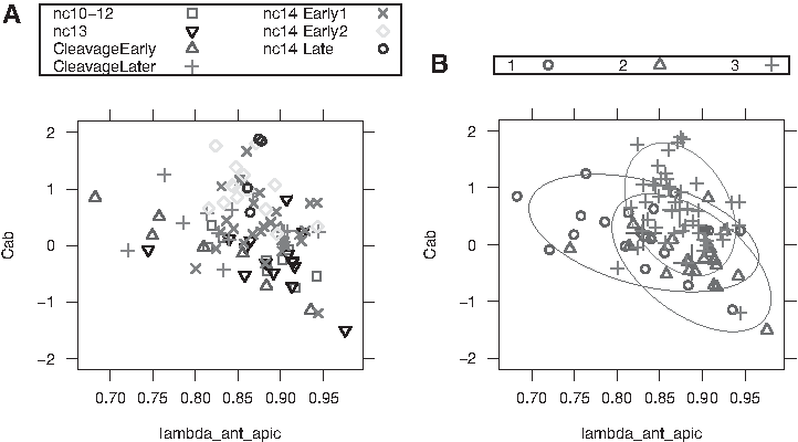
Log-ratio of two pre-exponential factors \documentclass{aastex}\usepackage{amsbsy}\usepackage{amsfonts}\usepackage{amssymb}\usepackage{bm}\usepackage{mathrsfs}\usepackage{pifont}\usepackage{stmaryrd}\usepackage{textcomp}\usepackage{portland, xspace}\usepackage{amsmath, amsxtra}\usepackage{upgreek}\pagestyle{empty}\DeclareMathSizes{10}{9}{7}{6}\begin{document} $${C^{ab}}$$ \end{document} versus anterior gradient \documentclass{aastex}\usepackage{amsbsy}\usepackage{amsfonts}\usepackage{amssymb}\usepackage{bm}\usepackage{mathrsfs}\usepackage{pifont}\usepackage{stmaryrd}\usepackage{textcomp}\usepackage{portland, xspace}\usepackage{amsmath, amsxtra}\usepackage{upgreek}\pagestyle{empty}\DeclareMathSizes{10}{9}{7}{6}\begin{document} $${ \rm{ \lambda }}_{{ \rm{anterior}}}^{ ( { \rm{apical}} ) }$$ \end{document} . (A) Seven (marked) developmental stages (Section 2.2): two-exponential parameters show large variability between and within the developmental stages. (B) Three combined groups: difference in parameter values, with 80% confidence ellipsoid.

Although the large variability and small sample size do not allow for statistically significant conclusions for all comparisons, several observations can be made. In particular, CleavageEarly has the largest average anterior exponential decay constant of any developmental stage (i.e., the steepest profile). This difference is statistically significant (t-test), but could be rendered insignificant by moderate changes in just one of the six embryos. We therefore combine groups to obtain three age groups (from 7) with larger sample sizes: (1) Cleavage, \documentclass{aastex}\usepackage{amsbsy}\usepackage{amsfonts}\usepackage{amssymb}\usepackage{bm}\usepackage{mathrsfs}\usepackage{pifont}\usepackage{stmaryrd}\usepackage{textcomp}\usepackage{portland, xspace}\usepackage{amsmath, amsxtra}\usepackage{upgreek}\pagestyle{empty}\DeclareMathSizes{10}{9}{7}{6}\begin{document} $$n = 20$$ \end{document} ; (2) nc10–nc13, \documentclass{aastex}\usepackage{amsbsy}\usepackage{amsfonts}\usepackage{amssymb}\usepackage{bm}\usepackage{mathrsfs}\usepackage{pifont}\usepackage{stmaryrd}\usepackage{textcomp}\usepackage{portland, xspace}\usepackage{amsmath, amsxtra}\usepackage{upgreek}\pagestyle{empty}\DeclareMathSizes{10}{9}{7}{6}\begin{document} $$n = 25$$ \end{document} ; (3) nc14, \documentclass{aastex}\usepackage{amsbsy}\usepackage{amsfonts}\usepackage{amssymb}\usepackage{bm}\usepackage{mathrsfs}\usepackage{pifont}\usepackage{stmaryrd}\usepackage{textcomp}\usepackage{portland, xspace}\usepackage{amsmath, amsxtra}\usepackage{upgreek}\pagestyle{empty}\DeclareMathSizes{10}{9}{7}{6}\begin{document} $$n = 47$$ \end{document} . Figure 3B shows that these larger groups have more distinct clustering, with distinct means.

Table 1 shows the average values for \documentclass{aastex}\usepackage{amsbsy}\usepackage{amsfonts}\usepackage{amssymb}\usepackage{bm}\usepackage{mathrsfs}\usepackage{pifont}\usepackage{stmaryrd}\usepackage{textcomp}\usepackage{portland, xspace}\usepackage{amsmath, amsxtra}\usepackage{upgreek}\pagestyle{empty}\DeclareMathSizes{10}{9}{7}{6}\begin{document} $${ \rm{ \lambda }}_{{ \rm{anterior}}}^{ ( { \rm{apical}} ) }$$ \end{document} and \documentclass{aastex}\usepackage{amsbsy}\usepackage{amsfonts}\usepackage{amssymb}\usepackage{bm}\usepackage{mathrsfs}\usepackage{pifont}\usepackage{stmaryrd}\usepackage{textcomp}\usepackage{portland, xspace}\usepackage{amsmath, amsxtra}\usepackage{upgreek}\pagestyle{empty}\DeclareMathSizes{10}{9}{7}{6}\begin{document} $${C^{ab}}$$ \end{document} with their 90% confidence intervals.

Table 1.

Combined Groups: Means and 90% Confidence Intervals for Main Characteristics of Apical and Basal Profiles for Three Groups

	\documentclass{aastex}\usepackage{amsbsy}\usepackage{amsfonts}\usepackage{amssymb}\usepackage{bm}\usepackage{mathrsfs}\usepackage{pifont}\usepackage{stmaryrd}\usepackage{textcomp}\usepackage{portland, xspace}\usepackage{amsmath, amsxtra}\usepackage{upgreek}\pagestyle{empty}\DeclareMathSizes{10}{9}{7}{6}\begin{document} $${ \rm{ \lambda }}_{{ \rm{anterior}}}^{ ( { \rm{apical}} ) }$$ \end{document}	Lower bound	Upper bound
Cleavage	0.831	0.803	0.859
nc10–13	0.887	0.870	0.904
nc14	0.874	0.865	0.883

	\documentclass{aastex}\usepackage{amsbsy}\usepackage{amsfonts}\usepackage{amssymb}\usepackage{bm}\usepackage{mathrsfs}\usepackage{pifont}\usepackage{stmaryrd}\usepackage{textcomp}\usepackage{portland, xspace}\usepackage{amsmath, amsxtra}\usepackage{upgreek}\pagestyle{empty}\DeclareMathSizes{10}{9}{7}{6}\begin{document} $${C^{{ \rm{ab}}}}$$ \end{document}	Lower bound	Upper bound
Cleavage	0.203	−0.010	0.417
nc10–13	−0.320	0.543	−0.096
nc14	0.618	0.461	0.775

One-way analysis of variance (both parametric and nonparametric; Kruskal–Wallis) confirms that both \documentclass{aastex}\usepackage{amsbsy}\usepackage{amsfonts}\usepackage{amssymb}\usepackage{bm}\usepackage{mathrsfs}\usepackage{pifont}\usepackage{stmaryrd}\usepackage{textcomp}\usepackage{portland, xspace}\usepackage{amsmath, amsxtra}\usepackage{upgreek}\pagestyle{empty}\DeclareMathSizes{10}{9}{7}{6}\begin{document} $${ \rm{ \lambda }}_{{ \rm{anterior}}}^{ ( { \rm{apical}} ) }$$ \end{document} and \documentclass{aastex}\usepackage{amsbsy}\usepackage{amsfonts}\usepackage{amssymb}\usepackage{bm}\usepackage{mathrsfs}\usepackage{pifont}\usepackage{stmaryrd}\usepackage{textcomp}\usepackage{portland, xspace}\usepackage{amsmath, amsxtra}\usepackage{upgreek}\pagestyle{empty}\DeclareMathSizes{10}{9}{7}{6}\begin{document} $${C^{ab}}$$ \end{document} significantly differ between the groups at the 5% level. Post-hoc comparisons show that \documentclass{aastex}\usepackage{amsbsy}\usepackage{amsfonts}\usepackage{amssymb}\usepackage{bm}\usepackage{mathrsfs}\usepackage{pifont}\usepackage{stmaryrd}\usepackage{textcomp}\usepackage{portland, xspace}\usepackage{amsmath, amsxtra}\usepackage{upgreek}\pagestyle{empty}\DeclareMathSizes{10}{9}{7}{6}\begin{document} $${C^{ab}}$$ \end{document} (the logarithm of the ratio between the apical and basal anterior gradients at 10%EL) is significantly different between all three groups; while the exponential decay rate of the anterior gradient is significantly larger ( \documentclass{aastex}\usepackage{amsbsy}\usepackage{amsfonts}\usepackage{amssymb}\usepackage{bm}\usepackage{mathrsfs}\usepackage{pifont}\usepackage{stmaryrd}\usepackage{textcomp}\usepackage{portland, xspace}\usepackage{amsmath, amsxtra}\usepackage{upgreek}\pagestyle{empty}\DeclareMathSizes{10}{9}{7}{6}\begin{document} $$\lambda$$ \end{document} is smaller) only for the Cleavage group.

3.3.1. Potentials of the approach

In Section 3.2, we screened embryos into type 1 using condition (A), that is, posteriorly non-increasing profiles. We can apply the suggested approach to embryos of type 2 with posteriorly increasing profiles (see Fig. 2B). Moreover, the model can be extended to three exponentials (see Fig. 4). With the extension of SSA to fit a three-exponential model, these sorts of patterns can be readily analyzed by the present approach, broadening the use of the technique to allow for the comparison of patterns from different genes [e.g., consider Stau protein (Spirov et al., 2009), which has a sharp rise in the vicinity of the posterior pole]. The article with biological results of application of the suggested approach, which includes a detailed description of the patterning dynamics in terms of the model parameters, is under preparation.

FIG. 4.

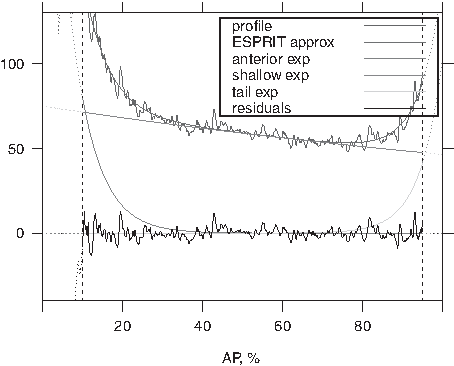
AP profile of the Stau protein [Cf. Spirov et al. (2009, fig. 6)]. The raw data are noisy; the smooth pattern is obtained by the 3-exponential model: anterior exponential 1, decreasing to zero from the left; shallow exponential 2, which is similar to a straight line; posterior exponential 3, increasing from zero to the right. The residual noise is oscillating around zero.

The approach presented here is likely to be an effective tool for quantifying other spatial gradients in developmental biology, which could aid in revealing new features in the patterning dynamics and regulation of critical developmental events, especially where there are large dynamic changes and high variability—that is, in cases where it is difficult to construct a reference or prototype profile. Examples include the dorsal gradient in DV Drosophila patterning (Kanodia et al., 2012, 2011; Reeves et al., 2012) and retinoic acid in vertebrate embryos (Schilling et al., 2012).

4. Conclusions

The new mathematical model described here enables the study of substantial quantitative problems in bcd mRNA gradient formation, including quantification of the between-embryo variability of the gradient; the filtering of atypical gradients; and the classification of embryos on the basis of quantitative gradient parameters. We are using these abilities to quantitatively study the dynamics of bcd mRNA profiles at very early stages of development. Finally, we can also now use the new mRNA gradient model to compare mRNA patterning with the Bcd protein gradient, previously analyzed in Alexandrov et al. (2008).

Footnotes

Acknowledgments

This work has been supported by U.S. NIH grant R01-GM072022 and the Russian Foundation for Basic Research grants 15-04-06480 and 16-04-00821.

Author Disclosure Statement

The authors declare that no competing financial interests exist.

References

Alexandrov

, Golyandina

, and Spirov

2008. Singular spectrum analysis of gene expression profiles of early Drosophila embryo: exponential-in-distance patterns. Res. Lett. Signal Process., 2008, 825758.

Ali-Murthy

, and Kornberg

2016. Bicoid gradient formation and function in the Drosophila pre-syncytial blastoderm. eLife. 5, e13222.

Alonso

, Castillo

, and Pintado

2005. Application of singular spectrum analysis to the smoothing of raw kinematic signals. J. Biomech., 38, 1085–1092.

Briscoe

, Lawrence

P.A.

, and Vincent

J.-P.

, eds. 2010. Generation and Interpretation of Morphogen Gradients: A Subject Collection from Cold Spring Harbor Perspectives in Biology. Cold Spring Harbor Laboratory Press, Cold Spring Harbor, NY.

Bullock

S.L.

, and Ish-Horowicz

2001. Conserved signals and machinery for RNA transport in Drosophila oogenesis and embryogenesis. Nature. 414, 611–616.

Cheung

, Miles

, Kreitman

, et al. 2011. Scaling of the Bicoid morphogen gradient by a volume-dependent production rate. Development. 138, 2741–2749.

Cheung

, Miles

, Kreitman

, et al. 2014. Adaptation of the length scale and amplitude of the Bicoid gradient profile to achieve robust patterning in abnormally large Drosophila melanogaster embryos. Development. 141, 124–135.

Dalessi

, Neves

, and Bergmann

2012. Modeling morphogen gradient formation from arbitrary realistically shaped sources. J. Theor. Biol., 294, 130–138.

Deng

, Wang

, Lu

L.J.

, et al. 2010. A two-dimensional simulation model of the bicoid gradient in Drosophila. PLoS One. 5, e10275.

10.

Fahmy

, Akber

, Cai

, et al. 2014.

\documentclass{aastex}\usepackage{amsbsy}\usepackage{amsfonts}\usepackage{amssymb}\usepackage{bm}\usepackage{mathrsfs}\usepackage{pifont}\usepackage{stmaryrd}\usepackage{textcomp}\usepackage{portland, xspace}\usepackage{amsmath, amsxtra}\usepackage{upgreek}\pagestyle{empty}\DeclareMathSizes{10}{9}{7}{6}\begin{document} $$\alpha$$ \end{document}

Tubulin 67C and Ncd are essential for establishing a cortical microtubular network and formation of the Bicoid mRNA gradient in Drosophila. PLoS One. 9, e112053.

11.

Golyandina

, Nekrutkin

, and Zhigljavsky

2001. Analysis of Time Series Structure: SSA and Related Techniques. Chapman&Hall/CRC, Boca Raton.

12.

Golyandina

, Pepelyshev

, and Steland

2012. New approaches to nonparametric density estimation and selection of smoothing parameters. Comput. Stat. Data Anal., 56, 2206–2218.

13.

Golyandina

, and Zhigljavsky

2013. Singular Spectrum Analysis for Time Series. Springer Briefs in Statistics. Springer Berlin Heidelberg.

14.

Grimm

, Coppey

, and Wieschaus

2010. Modelling the Bicoid gradient. Development. 137, 2253–2264.

15.

Holloway

D. H

, arrison

, Kosman

, et al. 2006. Analysis of pattern precision shows that Drosophila segmentation develops substantial independence from gradients of maternal gene products. Dev. Dyn., 235, 2949–2960.

16.

Houchmandzadeh

, Wieschaus

, and Leibler

2002. Establishment of developmental precision and proportions in the early Drosophila embryo. Nature. 415, 798–802.

17.

Kanodia

, Liang

H.-L.

, Kim

, et al. 2012. Pattern formation by graded and uniform signals in the early Drosophila embryo. Biophys. J., 102, 427–433.

18.

Kanodia

J.S.

, Kim

, Tomer

, et al. 2011. A computational statistics approach for estimating the spatial range of morphogen gradients. Development. 138, 4867–4874.

19.

Kavousanakis

M.E.

, Kanodia

J.S.

, Kim

, et al. 2010. A compartmental model for the Bicoid gradient. Dev. Biol., 345, 12–17.

20.

Lipshitz

H.D.

2009. Follow the mRNA: a new model for Bicoid gradient formation. Nat. Rev. Mol. Cell. Biol., 10, 509–512.

21.

Little

, Tkačik

, Kneeland

, et al. 2011. The formation of the Bicoid morphogen gradient requires protein movement from anteriorly localized mRNA. PLoS Biol. 9, e1000596.

22.

Liu

, and Niranjan

2012. Gaussian process modelling for bicoid mRNA regulation in spatio-temporal Bicoid profile. Bioinformatics. 28, 366–372.

23.

Myasnikova

, Samsonova

, Kosman

, et al. 2005. Removal of background signal from in situ data on the expression of segmentation genes in Drosophila. Dev. Genes Evol., 215, 320–326.

24.

Reeves

G.T.

, Trisnadi

, Truong

T.V.

, et al. 2012. Dorsal-ventral gene expression in the Drosophila embryo reflects the dynamics and precision of the dorsal nuclear gradient. Dev. Cell., 22, 544–557.

25.

Roy

, and Kailath

1989. ESPRIT: estimation of signal parameters via rotational invariance techniques. IEEE Trans. Acoust., 37, 984–995.

26.

Schilling

T.F.

, Nie

, and Lander

A.D.

2012. Dynamics and precision in retinoic acid morphogen gradients. Curr. Opin. Genet. Dev., 22, 562–569.

27.

Shlemov

, Golyandina

, Holloway

, et al. 2015a. Shaped 3D singular spectrum analysis for quantifying gene expression, with application to the early Drosophila embryo. Biomed. Res. Int., 2015, 1–18.

28.

Shlemov

, Golyandina

, Holloway

, et al. 2015b. Shaped singular spectrum analysis for quantifying gene expression, with application to the early Drosophila embryo. Biomed. Res. Int., 2015, 1–14.

29.

Spirov

, Fahmy

, Schneider

, et al. 2009. Formation of the bicoid morphogen gradient: an mRNA gradient dictates the protein gradient. Development. 136, 605–614.

30.

Spirov

A.V.

, Golyandina

N.E.

, Holloway

D.M.

, et al. 2012. Measuring gene expression noise in early Drosophila embryos: the highly dynamic compartmentalized micro-environment of the blastoderm is one of the main sources of noise, 177–188. In Giacobini

, Vanneschi

, Bush

W.S.

, eds. Evolutionary Computation, Machine Learning and Data Mining in Bioinformatics. EvoBIO 2012. Lecture Notes in Computer Science, Vol 7246. Springer, Berlin, Heidelberg.

31.

Surkova

, Kosman

, Kozlov

, et al. 2008. Characterization of the Drosophila segment determination morphome. Dev. Biol., 313, 844–862.

32.

Weil

T.T.

, Forrest

K.M.

, and Gavis

E.R.

2006. Localization of bicoid mRNA in late oocytes is maintained by continual active transport. Dev. Cell., 11, 251–262.

33.

Weil

T.T.

, Parton

, Davis

, et al. 2008. Changes in bicoid mRNA anchoring highlight conserved mechanisms during the oocyte-to-embryo transition. Curr. Biol., 18, 1055–1061.

Supplementary Material

Please find the following supplemental material available below.

For Open Access articles published under a Creative Commons License, all supplemental material carries the same license as the article it is associated with.

For non-Open Access articles published, all supplemental material carries a non-exclusive license, and permission requests for re-use of supplemental material or any part of supplemental material shall be sent directly to the copyright owner as specified in the copyright notice associated with the article.

0.00 MB

0.30 MB