Cancer arises from successive rounds of mutations, resulting in tumor cells with different somatic mutations known as clones. Drug responsiveness and therapeutics of cancer depend on the accurate detection of clones in a tumor sample. Recent research has considered inferring clonal composition of a tumor sample using computational models based on short read data of the sample generated using next-generation sequencing (NGS) technology. Short reads (segmented DNA parts of different tumor cells) are noisy; therefore, inferring the clones and their mutations from the data is a difficult and complex problem. We develop a new model called HetFHMM, based on factorial hidden Markov models, to infer clones and their proportions from noisy NGS data. In our model, each hidden chain represents the genomic signature of a clone, and a mixture of chains results in the observed data. We make use of Gibbs sampling and exponentiated gradient algorithms to infer the hidden variables and mixing proportions. We compare our model with strong models from previous work (PyClone and PhyloSub) based on both synthetic data and real cancer data on acute myeloid leukemia. Empirical results confirm that HetFHMM infers clonal composition of a tumor sample more accurately than previous work.
1. Introduction
Cancer is a genomic disease caused by somatic mutations accumulated in the genome during the lifetime of a human (Stratton et al., 2009). Somatic mutations create cells with genomic variations, known as clones, leading to a phenomenon called tumor heterogeneity (Ha et al., 2012). Recent cancer therapeutics have been developed to target cancer cells based on the mutations that they harbor (Caraco, 1998). From the treatment perspective, therefore, it is critical to identify genomic variations in cancer cells and clone-specific mutations composing a patient's tumor.
Next-generation sequencing (NGS) offers a great opportunity to identify clones in a tumor sample based on the generated short reads. NGS produces billions of short reads by chopping off the genome of cells into small segments and then conveniently reading these short sequences. It is challenging, however, to reconstruct back the genome of the sequenced cells since the short reads are not tagged with the ordering information. The difficulty of the problem is further exacerbated due to the mixing of short reads from cells belonging to different clones.
In this article, we present a statistical model to identify cancer clones and their genetic makeup from mixed and noisy short reads of a tumor sample. Our model discovers cancer clones harboring copy number variations (CNVs) and/or single-nucleotide variations (SNVs) as mutations. It allows mutations to belong to multiple clones, a phenomenon exhibited in cancer biology (Stratton et al., 2009), hence leading to more accurate modeling and prediction (c.f. experiments in Section 4). Furthermore, it infers the size of cancer clones through a notion called cellular prevalence, showing the relative number of cells belonging to a cancer clone in a tumor sample.
The problem of identifying clones and their mutations has recently attracted attention due to the viability of NGS technology. Global parameter hidden Markov model (Li et al., 2011) is a pioneering work to discover mutations involving CNVs and SNVs. It assumes that the tumor sample is a mixture of normal tissue and a tumor clone possessing all cancer-causing mutations. As discovered in cancer biology (Stratton et al., 2009), a tumor sample often has multiple clones and each clone harbors a subset of mutations in the tumor sample. This is the basis of Apolloh (Ha et al., 2012), Onco-SNP (Yau, 2013), and TH-HMM (Xia et al., 2013) in inferring CNVs and SNVs. To infer mutations, the aforementioned models assume the presence of three clones in a sample, where two of them are cancerous, and a mutation can appear in either of these cancer clones or both. TITAN (Ha et al., 2012) is an extension of Apolloh, which considers more than two cancer clones; however, it makes the assumption that a mutation cannot belong to more than one clone.
This limitation has been remedied in the follow-up works on PyClone (Roth et al., 2014), PhyloSub (Jiao et al., 2014), Rec-BTP (Hajirasouliha et al., 2014), PhyloWGS (Deshwar et al., 2015), and CITUP (Malikic et al., 2015) where they output the list of mutations characterizing each clone as well as the clonal frequency, that is, the percentage of tumor cells belonging to the clone. However, these models have two main drawbacks: (1) they are unable to discover different clones having the same clonal frequency and (2) they are not able to detect fine-grain composition of mutations, for example, if a genomic location harbors two mutations with different allelic composition. All of these limitations are addressed in our statistical model.
This article is organized as follows. In Section 2, we present our model called HetFHMM for detecting heterogeneity in cancer, which is based on factorial hidden Markov models (FHMMs). Given NGS short reads of a patient, we present the inference algorithm for predicting clonal frequency and genetic architecture. Since the gold-labeled data for this problem are not readily available, we then outline our evaluation setup in Section 4 to assess model predictions in this unsupervised learning scenario. We provide empirical results in Section 5 comparing our model against strong existing models from the literature on predicting clonal frequency and genetic makeup.
2. Model
Our goal is to identify the tumor clones and their genetic makeup from NGS short reads of a tumor sample. The genetic makeup of a clone is the set of mutations harbored by the clone and the genotype of those mutations. Table 1 lists all mutation genotypes that we consider; they not only represent a point mutation but also the copy number of the mutated part of the genome. The input to our model includes a list of mutated genome locations; the number of NGS short reads with match and mismatch nucleotides to the reference genome at those genomic locations; and the number of maximum clones believed to exist in the sample. The output of our model is then the set of mutations belonging to each clone, the genotype of those mutations in each clone, and the cellular frequency of each clone.
The basis of our model is that proximity on the genome induces interdependencies among mutations, in the sense that adjacent mutations tend to have similar genotypes and belong to the same clone (Ha et al., 2012). More specifically, we model each clone as a sequence of random variables where each of which corresponds to a mutated location on the genome. Each random variable takes a genotype as its value, and the genotypes of consecutive random variables are interdependent. These random variables are latent, but we note that they give rise to the observed counts from the data. We suggest a probabilistic graphical model that postulates a generative model of how the data are generated; we then reason about the latent variables of the model using statistical inference.
Let us assume that we are given a collection of T mutated genome locations to find the genetic makeup of a maximum of K clones. We denote the genotype of the clone k at the genomic location t by \documentclass{aastex}\usepackage{amsbsy}\usepackage{amsfonts}\usepackage{amssymb}\usepackage{bm}\usepackage{mathrsfs}\usepackage{pifont}\usepackage{stmaryrd}\usepackage{textcomp}\usepackage{portland, xspace}\usepackage{amsmath, amsxtra}\usepackage{upgreek}\pagestyle{empty}\DeclareMathSizes{10}{9}{7}{6}\begin{document}
$$G_t^k$$
\end{document}, and the cellular frequency of the clone k by \documentclass{aastex}\usepackage{amsbsy}\usepackage{amsfonts}\usepackage{amssymb}\usepackage{bm}\usepackage{mathrsfs}\usepackage{pifont}\usepackage{stmaryrd}\usepackage{textcomp}\usepackage{portland, xspace}\usepackage{amsmath, amsxtra}\usepackage{upgreek}\pagestyle{empty}\DeclareMathSizes{10}{9}{7}{6}\begin{document}
$${ \phi _k}$$
\end{document} where \documentclass{aastex}\usepackage{amsbsy}\usepackage{amsfonts}\usepackage{amssymb}\usepackage{bm}\usepackage{mathrsfs}\usepackage{pifont}\usepackage{stmaryrd}\usepackage{textcomp}\usepackage{portland, xspace}\usepackage{amsmath, amsxtra}\usepackage{upgreek}\pagestyle{empty}\DeclareMathSizes{10}{9}{7}{6}\begin{document}
$$\sum \nolimits_{k = 1}^K { \phi _k} = 1$$
\end{document}. We assume that clone 1 corresponds to normal cells, where the genotype for all genomic locations is AB where A and B represent the two alleles inherited from parents (Li et al., 2011). To infer the genotypes \documentclass{aastex}\usepackage{amsbsy}\usepackage{amsfonts}\usepackage{amssymb}\usepackage{bm}\usepackage{mathrsfs}\usepackage{pifont}\usepackage{stmaryrd}\usepackage{textcomp}\usepackage{portland, xspace}\usepackage{amsmath, amsxtra}\usepackage{upgreek}\pagestyle{empty}\DeclareMathSizes{10}{9}{7}{6}\begin{document}
$$G_t^k$$
\end{document} as well as cellular frequencies \documentclass{aastex}\usepackage{amsbsy}\usepackage{amsfonts}\usepackage{amssymb}\usepackage{bm}\usepackage{mathrsfs}\usepackage{pifont}\usepackage{stmaryrd}\usepackage{textcomp}\usepackage{portland, xspace}\usepackage{amsmath, amsxtra}\usepackage{upgreek}\pagestyle{empty}\DeclareMathSizes{10}{9}{7}{6}\begin{document}
$${ \phi _k}$$
\end{document}, the observed data for our model include the total short reads Nt covering the mutation t (aka the read depth), the number of matched at and mismatched bt short reads (note that \documentclass{aastex}\usepackage{amsbsy}\usepackage{amsfonts}\usepackage{amssymb}\usepackage{bm}\usepackage{mathrsfs}\usepackage{pifont}\usepackage{stmaryrd}\usepackage{textcomp}\usepackage{portland, xspace}\usepackage{amsmath, amsxtra}\usepackage{upgreek}\pagestyle{empty}\DeclareMathSizes{10}{9}{7}{6}\begin{document}
$${N_t} = {a_t} + {b_t}$$
\end{document}), and log ratio of the read depths in the tumor and normal samples.
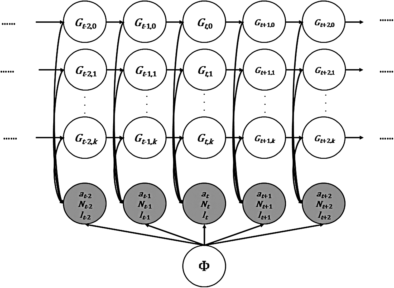
Our statistical model is based on FHMMs (Ghahramani and Jordan, 1997), where each chain corresponds to a clone and the observations correspond to the counts observed from NGS data (Fig. 1). In our model, henceforth referred to as HetFHMM, the joint probability of latent variables and observations is written as
\documentclass{aastex}\usepackage{amsbsy}\usepackage{amsfonts}\usepackage{amssymb}\usepackage{bm}\usepackage{mathrsfs}\usepackage{pifont}\usepackage{stmaryrd}\usepackage{textcomp}\usepackage{portland, xspace}\usepackage{amsmath, amsxtra}\usepackage{upgreek}\pagestyle{empty}\DeclareMathSizes{10}{9}{7}{6}\begin{document}
\begin{align*}
P ( \textbf{\textit{G}} , \textbf{\textit{O}} \vert \bm{\phi} ) = \left( { \left( { \prod \limits_{k = 1}^K P ( G_1^k ) } \right) P ( {\textbf{\textit{O}}_1} \vert {\textbf{\textit{G}}_1} , \bm{\phi} ) } \right) \left( { \prod \limits_{t = 2}^T { \left( { \prod \limits_{k = 1}^K P ( G_t^k \vert G_{t - 1}^k ) } \right) } P ( {\textbf{\textit{O}}_t} \vert {\textbf{\textit{G}}_t} , \bm{\phi} ) } \right) \tag{1}
\end{align*}
\end{document}
where \documentclass{aastex}\usepackage{amsbsy}\usepackage{amsfonts}\usepackage{amssymb}\usepackage{bm}\usepackage{mathrsfs}\usepackage{pifont}\usepackage{stmaryrd}\usepackage{textcomp}\usepackage{portland, xspace}\usepackage{amsmath, amsxtra}\usepackage{upgreek}\pagestyle{empty}\DeclareMathSizes{10}{9}{7}{6}\begin{document}
$${\textbf{\textit{G}}_t}$$
\end{document} is the vector of genotypes for all clones at mutation t, Ot is the observed data at mutation t, and \documentclass{aastex}\usepackage{amsbsy}\usepackage{amsfonts}\usepackage{amssymb}\usepackage{bm}\usepackage{mathrsfs}\usepackage{pifont}\usepackage{stmaryrd}\usepackage{textcomp}\usepackage{portland, xspace}\usepackage{amsmath, amsxtra}\usepackage{upgreek}\pagestyle{empty}\DeclareMathSizes{10}{9}{7}{6}\begin{document}
$$\bm{\phi}$$
\end{document} is the vector of cellular frequencies for all clones. Let us have a closer look into the elements of the model: (1) the term \documentclass{aastex}\usepackage{amsbsy}\usepackage{amsfonts}\usepackage{amssymb}\usepackage{bm}\usepackage{mathrsfs}\usepackage{pifont}\usepackage{stmaryrd}\usepackage{textcomp}\usepackage{portland, xspace}\usepackage{amsmath, amsxtra}\usepackage{upgreek}\pagestyle{empty}\DeclareMathSizes{10}{9}{7}{6}\begin{document}
$$P ( G_t^k \vert G_{t - 1}^k )$$
\end{document} is called the transition probability and determines the dependency of the genotype of the next mutation conditioned on that of the current mutation and (2) the term \documentclass{aastex}\usepackage{amsbsy}\usepackage{amsfonts}\usepackage{amssymb}\usepackage{bm}\usepackage{mathrsfs}\usepackage{pifont}\usepackage{stmaryrd}\usepackage{textcomp}\usepackage{portland, xspace}\usepackage{amsmath, amsxtra}\usepackage{upgreek}\pagestyle{empty}\DeclareMathSizes{10}{9}{7}{6}\begin{document}
$$P ( {\textbf{\textit{O}}_t} \vert {\textbf{\textit{G}}_t} , \bm{\phi} )$$
\end{document} is called the emission probability and determines the relationship of the observed data \documentclass{aastex}\usepackage{amsbsy}\usepackage{amsfonts}\usepackage{amssymb}\usepackage{bm}\usepackage{mathrsfs}\usepackage{pifont}\usepackage{stmaryrd}\usepackage{textcomp}\usepackage{portland, xspace}\usepackage{amsmath, amsxtra}\usepackage{upgreek}\pagestyle{empty}\DeclareMathSizes{10}{9}{7}{6}\begin{document}
$${\textbf{\textit{O}}_t}$$
\end{document} and latent variables \documentclass{aastex}\usepackage{amsbsy}\usepackage{amsfonts}\usepackage{amssymb}\usepackage{bm}\usepackage{mathrsfs}\usepackage{pifont}\usepackage{stmaryrd}\usepackage{textcomp}\usepackage{portland, xspace}\usepackage{amsmath, amsxtra}\usepackage{upgreek}\pagestyle{empty}\DeclareMathSizes{10}{9}{7}{6}\begin{document}
$${\textbf{\textit{G}}_t}$$
\end{document} at mutation t (conditioned on cellular frequencies \documentclass{aastex}\usepackage{amsbsy}\usepackage{amsfonts}\usepackage{amssymb}\usepackage{bm}\usepackage{mathrsfs}\usepackage{pifont}\usepackage{stmaryrd}\usepackage{textcomp}\usepackage{portland, xspace}\usepackage{amsmath, amsxtra}\usepackage{upgreek}\pagestyle{empty}\DeclareMathSizes{10}{9}{7}{6}\begin{document}
$${ \bm{\phi} _t}$$
\end{document}). In what follows, we provide an in-depth explanation of these terms.
The probabilistic graphical model of our Factorial Hidden Markov Model for analyzing heterogeneity (HetFHMM).
2.1. Transition probability
The transition probability \documentclass{aastex}\usepackage{amsbsy}\usepackage{amsfonts}\usepackage{amssymb}\usepackage{bm}\usepackage{mathrsfs}\usepackage{pifont}\usepackage{stmaryrd}\usepackage{textcomp}\usepackage{portland, xspace}\usepackage{amsmath, amsxtra}\usepackage{upgreek}\pagestyle{empty}\DeclareMathSizes{10}{9}{7}{6}\begin{document}
$$P ( G_t^k = i \vert G_{t - 1}^k = j )$$
\end{document}, which is denoted by \documentclass{aastex}\usepackage{amsbsy}\usepackage{amsfonts}\usepackage{amssymb}\usepackage{bm}\usepackage{mathrsfs}\usepackage{pifont}\usepackage{stmaryrd}\usepackage{textcomp}\usepackage{portland, xspace}\usepackage{amsmath, amsxtra}\usepackage{upgreek}\pagestyle{empty}\DeclareMathSizes{10}{9}{7}{6}\begin{document}
$$A_t^k ( i , j )$$
\end{document} from the transition matrix \documentclass{aastex}\usepackage{amsbsy}\usepackage{amsfonts}\usepackage{amssymb}\usepackage{bm}\usepackage{mathrsfs}\usepackage{pifont}\usepackage{stmaryrd}\usepackage{textcomp}\usepackage{portland, xspace}\usepackage{amsmath, amsxtra}\usepackage{upgreek}\pagestyle{empty}\DeclareMathSizes{10}{9}{7}{6}\begin{document}
$$A_t^k$$
\end{document}, captures the interdependencies between genotypes of adjacent mutations. Following Colella et al. (2007), we define the transition matrix for each chain as follows:
\documentclass{aastex}\usepackage{amsbsy}\usepackage{amsfonts}\usepackage{amssymb}\usepackage{bm}\usepackage{mathrsfs}\usepackage{pifont}\usepackage{stmaryrd}\usepackage{textcomp}\usepackage{portland, xspace}\usepackage{amsmath, amsxtra}\usepackage{upgreek}\pagestyle{empty}\DeclareMathSizes{10}{9}{7}{6}\begin{document}
\begin{align*}
\underbrace {P ( G_t^k = i \vert G_{t - 1}^k = j ) }_{A_t^k ( i , j ) } = \left\{ { \begin{matrix} {{ \rho _t}} \hfill & { \quad { \rm{if }}i{ \rm{ = }}j} \hfill \\ {{{1 - { \rho _t}} \over {{D_k} - 1}}} \hfill & { \quad { \rm{Otherwise}}{ \rm{.}}} \hfill \\ \end{matrix} } \right. \tag{2}
\end{align*}
\end{document}
The stickiness of the genotype Markov process \documentclass{aastex}\usepackage{amsbsy}\usepackage{amsfonts}\usepackage{amssymb}\usepackage{bm}\usepackage{mathrsfs}\usepackage{pifont}\usepackage{stmaryrd}\usepackage{textcomp}\usepackage{portland, xspace}\usepackage{amsmath, amsxtra}\usepackage{upgreek}\pagestyle{empty}\DeclareMathSizes{10}{9}{7}{6}\begin{document}
$${ \rho _t}$$
\end{document} is defined as
\documentclass{aastex}\usepackage{amsbsy}\usepackage{amsfonts}\usepackage{amssymb}\usepackage{bm}\usepackage{mathrsfs}\usepackage{pifont}\usepackage{stmaryrd}\usepackage{textcomp}\usepackage{portland, xspace}\usepackage{amsmath, amsxtra}\usepackage{upgreek}\pagestyle{empty}\DeclareMathSizes{10}{9}{7}{6}\begin{document}
\begin{align*}
{ \rho _t } = 1 - \frac { 1 } { 2 } \left( 1 - { e^ { \frac { { - { d_t } } } { L } } } \right) \tag { 3 }
\end{align*}
\end{document}
where L is the average length of the sequence reads,*Dk is the dimension of the state space (i.e., the number of genotypes, which is 21 from Table 1), and dk is the genomic distance between the mutant locations t and \documentclass{aastex}\usepackage{amsbsy}\usepackage{amsfonts}\usepackage{amssymb}\usepackage{bm}\usepackage{mathrsfs}\usepackage{pifont}\usepackage{stmaryrd}\usepackage{textcomp}\usepackage{portland, xspace}\usepackage{amsmath, amsxtra}\usepackage{upgreek}\pagestyle{empty}\DeclareMathSizes{10}{9}{7}{6}\begin{document}
$$t - 1$$
\end{document}.
2.2. Emission probability
We decompose the emission probability for generating the observation \documentclass{aastex}\usepackage{amsbsy}\usepackage{amsfonts}\usepackage{amssymb}\usepackage{bm}\usepackage{mathrsfs}\usepackage{pifont}\usepackage{stmaryrd}\usepackage{textcomp}\usepackage{portland, xspace}\usepackage{amsmath, amsxtra}\usepackage{upgreek}\pagestyle{empty}\DeclareMathSizes{10}{9}{7}{6}\begin{document}
$${\textbf{\textit{O}}_t}$$
\end{document} based on the hidden variables \documentclass{aastex}\usepackage{amsbsy}\usepackage{amsfonts}\usepackage{amssymb}\usepackage{bm}\usepackage{mathrsfs}\usepackage{pifont}\usepackage{stmaryrd}\usepackage{textcomp}\usepackage{portland, xspace}\usepackage{amsmath, amsxtra}\usepackage{upgreek}\pagestyle{empty}\DeclareMathSizes{10}{9}{7}{6}\begin{document}
$${\textbf{\textit{G}}_t}$$
\end{document} and \documentclass{aastex}\usepackage{amsbsy}\usepackage{amsfonts}\usepackage{amssymb}\usepackage{bm}\usepackage{mathrsfs}\usepackage{pifont}\usepackage{stmaryrd}\usepackage{textcomp}\usepackage{portland, xspace}\usepackage{amsmath, amsxtra}\usepackage{upgreek}\pagestyle{empty}\DeclareMathSizes{10}{9}{7}{6}\begin{document}
$$\bm{\phi}$$
\end{document} as follows:
\documentclass{aastex}\usepackage{amsbsy}\usepackage{amsfonts}\usepackage{amssymb}\usepackage{bm}\usepackage{mathrsfs}\usepackage{pifont}\usepackage{stmaryrd}\usepackage{textcomp}\usepackage{portland, xspace}\usepackage{amsmath, amsxtra}\usepackage{upgreek}\pagestyle{empty}\DeclareMathSizes{10}{9}{7}{6}\begin{document}
\begin{align*}
P ( {\textbf{\textit{O}}_t} \vert {\textbf{\textit{G}}_t} , { \bm{\phi}} ) = P ( {a_t} \vert {N_t} , {\textbf{\textit{G}}_t} , \bm{\phi} ) P ( {l_t} \vert {\textbf{\textit{G}}_t} , \bm{\phi} ) \tag{4}
\end{align*}
\end{document}
where at, Nt, and lt are defined as before. We now elaborate the above two terms in the emission probability.
Following previous work (Ha et al., 2012), we assume that at follows binomial distribution where the number of trials is Nt and the probability of success is as follows:
\documentclass{aastex}\usepackage{amsbsy}\usepackage{amsfonts}\usepackage{amssymb}\usepackage{bm}\usepackage{mathrsfs}\usepackage{pifont}\usepackage{stmaryrd}\usepackage{textcomp}\usepackage{portland, xspace}\usepackage{amsmath, amsxtra}\usepackage{upgreek}\pagestyle{empty}\DeclareMathSizes{10}{9}{7}{6}\begin{document}
\begin{align*}
{ P_ { { b_t } } } = { \frac { \sum \nolimits_ { k = 1 } ^K { { \phi _k } . { r_ { g_t^k } } } } { \sum \nolimits_ { k = 1 } ^K { { \phi _k } . { c_ { g_t^k } } } } } \tag { 5 }
\end{align*}
\end{document}
where \documentclass{aastex}\usepackage{amsbsy}\usepackage{amsfonts}\usepackage{amssymb}\usepackage{bm}\usepackage{mathrsfs}\usepackage{pifont}\usepackage{stmaryrd}\usepackage{textcomp}\usepackage{portland, xspace}\usepackage{amsmath, amsxtra}\usepackage{upgreek}\pagestyle{empty}\DeclareMathSizes{10}{9}{7}{6}\begin{document}
$${r_{g_t^k}}$$
\end{document} and \documentclass{aastex}\usepackage{amsbsy}\usepackage{amsfonts}\usepackage{amssymb}\usepackage{bm}\usepackage{mathrsfs}\usepackage{pifont}\usepackage{stmaryrd}\usepackage{textcomp}\usepackage{portland, xspace}\usepackage{amsmath, amsxtra}\usepackage{upgreek}\pagestyle{empty}\DeclareMathSizes{10}{9}{7}{6}\begin{document}
$${c_{g_t^k}}$$
\end{document} are number of reference allele and the copy number of the genotype in \documentclass{aastex}\usepackage{amsbsy}\usepackage{amsfonts}\usepackage{amssymb}\usepackage{bm}\usepackage{mathrsfs}\usepackage{pifont}\usepackage{stmaryrd}\usepackage{textcomp}\usepackage{portland, xspace}\usepackage{amsmath, amsxtra}\usepackage{upgreek}\pagestyle{empty}\DeclareMathSizes{10}{9}{7}{6}\begin{document}
$$G_t^k$$
\end{document}. For example, if the genotype is AAB, then \documentclass{aastex}\usepackage{amsbsy}\usepackage{amsfonts}\usepackage{amssymb}\usepackage{bm}\usepackage{mathrsfs}\usepackage{pifont}\usepackage{stmaryrd}\usepackage{textcomp}\usepackage{portland, xspace}\usepackage{amsmath, amsxtra}\usepackage{upgreek}\pagestyle{empty}\DeclareMathSizes{10}{9}{7}{6}\begin{document}
$${r_{g_t^k}} = 2$$
\end{document} and \documentclass{aastex}\usepackage{amsbsy}\usepackage{amsfonts}\usepackage{amssymb}\usepackage{bm}\usepackage{mathrsfs}\usepackage{pifont}\usepackage{stmaryrd}\usepackage{textcomp}\usepackage{portland, xspace}\usepackage{amsmath, amsxtra}\usepackage{upgreek}\pagestyle{empty}\DeclareMathSizes{10}{9}{7}{6}\begin{document}
$${c_{g_t^k}} = 3$$
\end{document}.
The number of the short reads of tumor and normal cells is more than a billion. As per the central limit theorem, it is assumed that the log ratio of tumor-normal read depth is Gaussian distributed with mean \documentclass{aastex}\usepackage{amsbsy}\usepackage{amsfonts}\usepackage{amssymb}\usepackage{bm}\usepackage{mathrsfs}\usepackage{pifont}\usepackage{stmaryrd}\usepackage{textcomp}\usepackage{portland, xspace}\usepackage{amsmath, amsxtra}\usepackage{upgreek}\pagestyle{empty}\DeclareMathSizes{10}{9}{7}{6}\begin{document}
$${ \mu _t}$$
\end{document} and standard deviation \documentclass{aastex}\usepackage{amsbsy}\usepackage{amsfonts}\usepackage{amssymb}\usepackage{bm}\usepackage{mathrsfs}\usepackage{pifont}\usepackage{stmaryrd}\usepackage{textcomp}\usepackage{portland, xspace}\usepackage{amsmath, amsxtra}\usepackage{upgreek}\pagestyle{empty}\DeclareMathSizes{10}{9}{7}{6}\begin{document}
$$\sigma$$
\end{document}. Mean of the log ratio of tumor-normal read depth is
\documentclass{aastex}\usepackage{amsbsy}\usepackage{amsfonts}\usepackage{amssymb}\usepackage{bm}\usepackage{mathrsfs}\usepackage{pifont}\usepackage{stmaryrd}\usepackage{textcomp}\usepackage{portland, xspace}\usepackage{amsmath, amsxtra}\usepackage{upgreek}\pagestyle{empty}\DeclareMathSizes{10}{9}{7}{6}\begin{document}
\begin{align*}
{ \mu _t } = { \frac { \sum \nolimits_ { i = 0 } ^K { { \phi _k } . { c_ { g_t^k } } } } { { \phi _0 } . { c_ { g_t^0 } } . \sum \nolimits_ { i = 1 } ^K { { \phi _i } . \psi } } } \tag { 6 }
\end{align*}
\end{document}
where \documentclass{aastex}\usepackage{amsbsy}\usepackage{amsfonts}\usepackage{amssymb}\usepackage{bm}\usepackage{mathrsfs}\usepackage{pifont}\usepackage{stmaryrd}\usepackage{textcomp}\usepackage{portland, xspace}\usepackage{amsmath, amsxtra}\usepackage{upgreek}\pagestyle{empty}\DeclareMathSizes{10}{9}{7}{6}\begin{document}
$$\psi$$
\end{document} is the tumor ploidy† parameter that is set to 3.
We repeatedly alternate between inferring the clone-specific genotypes and the cellular prevalence until the convergence condition is met, that is, we alternate between \documentclass{aastex}\usepackage{amsbsy}\usepackage{amsfonts}\usepackage{amssymb}\usepackage{bm}\usepackage{mathrsfs}\usepackage{pifont}\usepackage{stmaryrd}\usepackage{textcomp}\usepackage{portland, xspace}\usepackage{amsmath, amsxtra}\usepackage{upgreek}\pagestyle{empty}\DeclareMathSizes{10}{9}{7}{6}\begin{document}
$$\bm{\phi}$$
\end{document} and \documentclass{aastex}\usepackage{amsbsy}\usepackage{amsfonts}\usepackage{amssymb}\usepackage{bm}\usepackage{mathrsfs}\usepackage{pifont}\usepackage{stmaryrd}\usepackage{textcomp}\usepackage{portland, xspace}\usepackage{amsmath, amsxtra}\usepackage{upgreek}\pagestyle{empty}\DeclareMathSizes{10}{9}{7}{6}\begin{document}
$$\textbf{\textit{G}}$$
\end{document} to maximize the above likelihood function. In what follows, we elaborate on these two phases of our optimization algorithm.
3.1. Optimizing \documentclass{aastex}\usepackage{amsbsy}\usepackage{amsfonts}\usepackage{amssymb}\usepackage{bm}\usepackage{mathrsfs}\usepackage{pifont}\usepackage{stmaryrd}\usepackage{textcomp}\usepackage{portland, xspace}\usepackage{amsmath, amsxtra}\usepackage{upgreek}\pagestyle{empty}\DeclareMathSizes{10}{9}{7}{6}\begin{document}
$$\bm{\phi}$$
\end{document} while \documentclass{aastex}\usepackage{amsbsy}\usepackage{amsfonts}\usepackage{amssymb}\usepackage{bm}\usepackage{mathrsfs}\usepackage{pifont}\usepackage{stmaryrd}\usepackage{textcomp}\usepackage{portland, xspace}\usepackage{amsmath, amsxtra}\usepackage{upgreek}\pagestyle{empty}\DeclareMathSizes{10}{9}{7}{6}\begin{document}
$$\textbf{\textit{G}}$$
\end{document} is fixed
Maximizing the likelihood function over \documentclass{aastex}\usepackage{amsbsy}\usepackage{amsfonts}\usepackage{amssymb}\usepackage{bm}\usepackage{mathrsfs}\usepackage{pifont}\usepackage{stmaryrd}\usepackage{textcomp}\usepackage{portland, xspace}\usepackage{amsmath, amsxtra}\usepackage{upgreek}\pagestyle{empty}\DeclareMathSizes{10}{9}{7}{6}\begin{document}
$$\bm{\phi}$$
\end{document} is a constrained optimization problem since \documentclass{aastex}\usepackage{amsbsy}\usepackage{amsfonts}\usepackage{amssymb}\usepackage{bm}\usepackage{mathrsfs}\usepackage{pifont}\usepackage{stmaryrd}\usepackage{textcomp}\usepackage{portland, xspace}\usepackage{amsmath, amsxtra}\usepackage{upgreek}\pagestyle{empty}\DeclareMathSizes{10}{9}{7}{6}\begin{document}
$$\bm{\phi}$$
\end{document} is constrained to be a probability vector, that is, \documentclass{aastex}\usepackage{amsbsy}\usepackage{amsfonts}\usepackage{amssymb}\usepackage{bm}\usepackage{mathrsfs}\usepackage{pifont}\usepackage{stmaryrd}\usepackage{textcomp}\usepackage{portland, xspace}\usepackage{amsmath, amsxtra}\usepackage{upgreek}\pagestyle{empty}\DeclareMathSizes{10}{9}{7}{6}\begin{document}
$$\sum \nolimits_k { \phi _k} = 1$$
\end{document} and \documentclass{aastex}\usepackage{amsbsy}\usepackage{amsfonts}\usepackage{amssymb}\usepackage{bm}\usepackage{mathrsfs}\usepackage{pifont}\usepackage{stmaryrd}\usepackage{textcomp}\usepackage{portland, xspace}\usepackage{amsmath, amsxtra}\usepackage{upgreek}\pagestyle{empty}\DeclareMathSizes{10}{9}{7}{6}\begin{document}
$${ \phi _k}$$
\end{document} are non-negative. We make use of the exponentiated gradient (EG) algorithm to solve this constrained optimization problem.
More formally, the constrained optimization problem is as follows:
\documentclass{aastex}\usepackage{amsbsy}\usepackage{amsfonts}\usepackage{amssymb}\usepackage{bm}\usepackage{mathrsfs}\usepackage{pifont}\usepackage{stmaryrd}\usepackage{textcomp}\usepackage{portland, xspace}\usepackage{amsmath, amsxtra}\usepackage{upgreek}\pagestyle{empty}\DeclareMathSizes{10}{9}{7}{6}\begin{document}
\begin{align*}
\mathop { \min } \limits_{ \bm{\phi} \in \Delta } - \mathcal{L} ( \bm{\phi} ) \tag{8}
\end{align*}
\end{document}
where \documentclass{aastex}\usepackage{amsbsy}\usepackage{amsfonts}\usepackage{amssymb}\usepackage{bm}\usepackage{mathrsfs}\usepackage{pifont}\usepackage{stmaryrd}\usepackage{textcomp}\usepackage{portland, xspace}\usepackage{amsmath, amsxtra}\usepackage{upgreek}\pagestyle{empty}\DeclareMathSizes{10}{9}{7}{6}\begin{document}
$$\mathcal{L} ( \bm{\phi} ) = - \log P ( \textbf{\textit{G}} , \textbf{\textit{l}} , \textbf{\textit{a}} \vert \bm{\phi} , \textbf{\textit{N}} , \sigma )$$
\end{document} and \documentclass{aastex}\usepackage{amsbsy}\usepackage{amsfonts}\usepackage{amssymb}\usepackage{bm}\usepackage{mathrsfs}\usepackage{pifont}\usepackage{stmaryrd}\usepackage{textcomp}\usepackage{portland, xspace}\usepackage{amsmath, amsxtra}\usepackage{upgreek}\pagestyle{empty}\DeclareMathSizes{10}{9}{7}{6}\begin{document}
$$\Delta$$
\end{document} is the simplex containing all probability vectors. To solve the above minimization problem, the EG updates are as follows:
\documentclass{aastex}\usepackage{amsbsy}\usepackage{amsfonts}\usepackage{amssymb}\usepackage{bm}\usepackage{mathrsfs}\usepackage{pifont}\usepackage{stmaryrd}\usepackage{textcomp}\usepackage{portland, xspace}\usepackage{amsmath, amsxtra}\usepackage{upgreek}\pagestyle{empty}\DeclareMathSizes{10}{9}{7}{6}\begin{document}
\begin{align*}
\phi _k^{new} \propto { \phi _k}{e^{ - ( \eta { \nabla _{{ \phi _k}}} \mathcal{L} ( \bm{\phi} ) ) }} \tag{9}
\end{align*}
\end{document}
where \documentclass{aastex}\usepackage{amsbsy}\usepackage{amsfonts}\usepackage{amssymb}\usepackage{bm}\usepackage{mathrsfs}\usepackage{pifont}\usepackage{stmaryrd}\usepackage{textcomp}\usepackage{portland, xspace}\usepackage{amsmath, amsxtra}\usepackage{upgreek}\pagestyle{empty}\DeclareMathSizes{10}{9}{7}{6}\begin{document}
$$\eta$$
\end{document} is the learning rate. After updating each component of the latent vector \documentclass{aastex}\usepackage{amsbsy}\usepackage{amsfonts}\usepackage{amssymb}\usepackage{bm}\usepackage{mathrsfs}\usepackage{pifont}\usepackage{stmaryrd}\usepackage{textcomp}\usepackage{portland, xspace}\usepackage{amsmath, amsxtra}\usepackage{upgreek}\pagestyle{empty}\DeclareMathSizes{10}{9}{7}{6}\begin{document}
$$\bm{\phi}$$
\end{document}, the values are normalized so that they sum to one. For the EG updates, we need the derivatives that are derived using the chain rule in Appendix A.
3.2. Optimizing \documentclass{aastex}\usepackage{amsbsy}\usepackage{amsfonts}\usepackage{amssymb}\usepackage{bm}\usepackage{mathrsfs}\usepackage{pifont}\usepackage{stmaryrd}\usepackage{textcomp}\usepackage{portland, xspace}\usepackage{amsmath, amsxtra}\usepackage{upgreek}\pagestyle{empty}\DeclareMathSizes{10}{9}{7}{6}\begin{document}
$${ \bf{G}}$$
\end{document} while \documentclass{aastex}\usepackage{amsbsy}\usepackage{amsfonts}\usepackage{amssymb}\usepackage{bm}\usepackage{mathrsfs}\usepackage{pifont}\usepackage{stmaryrd}\usepackage{textcomp}\usepackage{portland, xspace}\usepackage{amsmath, amsxtra}\usepackage{upgreek}\pagestyle{empty}\DeclareMathSizes{10}{9}{7}{6}\begin{document}
$$\bm{\phi}$$
\end{document} is fixed
Since the exact inference in FHMM is intractable (Ghahramani and Jordan, 1997), we make use of Gibbs sampling as a Markov chain Monte Carlo method for approximate inference. Initially, we choose uniformly at random a genotype value for genotype variables in all chains except the normal chain where the genotypes are fixed to AB. Then, we sample each variable while the states of the rest of the variables are fixed. That is, the posterior probability of each genotype for a hidden variable \documentclass{aastex}\usepackage{amsbsy}\usepackage{amsfonts}\usepackage{amssymb}\usepackage{bm}\usepackage{mathrsfs}\usepackage{pifont}\usepackage{stmaryrd}\usepackage{textcomp}\usepackage{portland, xspace}\usepackage{amsmath, amsxtra}\usepackage{upgreek}\pagestyle{empty}\DeclareMathSizes{10}{9}{7}{6}\begin{document}
$${G_{t , k}}$$
\end{document} is
\documentclass{aastex}\usepackage{amsbsy}\usepackage{amsfonts}\usepackage{amssymb}\usepackage{bm}\usepackage{mathrsfs}\usepackage{pifont}\usepackage{stmaryrd}\usepackage{textcomp}\usepackage{portland, xspace}\usepackage{amsmath, amsxtra}\usepackage{upgreek}\pagestyle{empty}\DeclareMathSizes{10}{9}{7}{6}\begin{document}
\begin{align*}
P ( {G_{t , k}} ) \propto {A_t} ( {G_{t , k}} \vert {G_{t - 1 , k}} ) {A_{t + 1}} ( {G_{t + 1 , k}} \vert {G_{t , k}} ) \times \mathcal{B}in ( {a_t} \vert {N_t} , {P_{{b_t}}} ) { \cal N} ( {l_t} \vert { \mu _t} , \sigma ) \tag{10}
\end{align*}
\end{document}
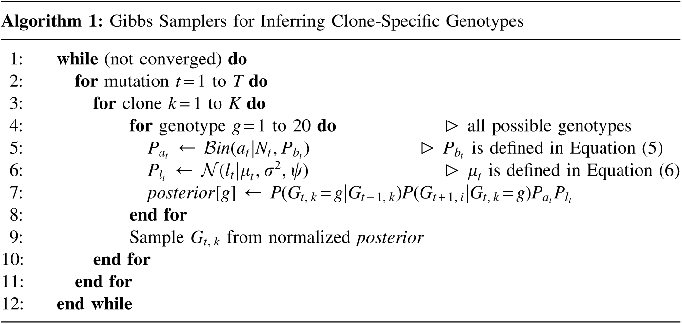
The Gibbs sampling algorithm is shown in Algorithm 1.
4. Evaluation Framework
No existing model infers tumor clones and their genomic makeup along with the cellular prevalence from tumor samples. Hence, it is challenging to evaluate our model due to the lack of (1) appropriate data annotated with clones' details, (2) the most compatible models for comparison, and (3) suitable evaluation metrics. We focus on these issues in the rest of this section.
4.1. Real and synthetic data
4.1.1. Real cancer data
We make use of laboratory experimented acute myeloid leukemia (AML) (Ding et al., 2012) as the real data. The data include samples of seven patients, which were obtained after chemotherapy treatment. The data are annotated with the clones and their mutations based on laboratory experiments, which we use as the gold standard; however, the annotation does not include the cellular prevalence of the clones.
4.1.2. Synthetic cancer data
To assess different aspects of our model, we generate synthetic cancer data containing the clone-specific genotypes and their cellular prevalence (Table 2); Algorithm 2 summarizes the process. To generate synthetic data, we first specify the number of clones and their cellular prevalences. We then generate the location of mutations on the genome. After randomly generating the location of the first mutation, we generate the gap between two consecutive mutations from a uniform distribution on (6K, 7K) since the average distance between two consecutive mutations in the AML data is 6679 base pairs (Ding et al., 2012). After generating the locations, genotypes and observations are sampled based on Equations (2) and (4), respectively.
Clone Configurations for the Synthetic Data
Tumor clones
Configuration
Clone data
Normal tissue
1
2
3
4
5
6
7
1
3
0.20
0.28
0.52
—
—
—
—
—
4
0.10
0.04
0.30
0.65
—
—
—
—
5
0.01
0.05
0.12
0.22
0.60
—
—
—
6
0.01
0.04
0.08
0.13
0.25
0.49
—
—
8
0.01
0.02
0.04
0.07
0.13
0.15
0.22
0.36
1
3
0.30
0.20
0.50
—
—
—
—
—
4
0.20
0.08
0.12
0.60
—
—
—
—
5
0.18
0.06
0.09
0.15
0.52
—
—
—
6
0.17
0.04
0.08
0.11
0.13
0.47
—
—
8
0.15
0.02
0.04
0.06
0.08
0.10
0.13
0.42
1
3
0.17
0.38
0.45
—
—
—
—
—
4
0.20
0.12
0.12
0.56
—
—
—
—
5
0.11
0.11
0.11
0.15
0.54
—
—
—
6
0.09
0.10
0.11
0.12
0.13
0.45
—
—
8
0.03
0.05
0.07
0.09
0.10
0.10
0.16
0.40
We would like to assess our model in data conditions where the interdependency assumptions made in the model about adjacent genotypes do not hold. Therefore, we generate two more versions of the aforementioned datasets where the gap dt in computation of the stickiness of the genotype Markov process \documentclass{aastex}\usepackage{amsbsy}\usepackage{amsfonts}\usepackage{amssymb}\usepackage{bm}\usepackage{mathrsfs}\usepackage{pifont}\usepackage{stmaryrd}\usepackage{textcomp}\usepackage{portland, xspace}\usepackage{amsmath, amsxtra}\usepackage{upgreek}\pagestyle{empty}\DeclareMathSizes{10}{9}{7}{6}\begin{document}
$${ \rho _t}$$
\end{document} in Equation (3) is scaled by 3 and 1/3, which correspond to stronger and weaker interdependencies, respectively. This also provides a compelling test bed for comparison against the competing models, PyClone and PhyloSub, which assume no dependency between genotypes of adjacent mutations.
Algorithm 2: Synthetic Data Generation Algorithm
1:
Specify the cellular prevalence of clones \documentclass{aastex}\usepackage{amsbsy}\usepackage{amsfonts}\usepackage{amssymb}\usepackage{bm}\usepackage{mathrsfs}\usepackage{pifont}\usepackage{stmaryrd}\usepackage{textcomp}\usepackage{portland, xspace}\usepackage{amsmath, amsxtra}\usepackage{upgreek}\pagestyle{empty}\DeclareMathSizes{10}{9}{7}{6}\begin{document}
$$\Phi$$
\end{document}
2:
Generate mutation locations {1, …, T}
▹ refer to the text
3:
Set \documentclass{aastex}\usepackage{amsbsy}\usepackage{amsfonts}\usepackage{amssymb}\usepackage{bm}\usepackage{mathrsfs}\usepackage{pifont}\usepackage{stmaryrd}\usepackage{textcomp}\usepackage{portland, xspace}\usepackage{amsmath, amsxtra}\usepackage{upgreek}\pagestyle{empty}\DeclareMathSizes{10}{9}{7}{6}\begin{document}
$${G_{1 , 1}}$$
\end{document} .… \documentclass{aastex}\usepackage{amsbsy}\usepackage{amsfonts}\usepackage{amssymb}\usepackage{bm}\usepackage{mathrsfs}\usepackage{pifont}\usepackage{stmaryrd}\usepackage{textcomp}\usepackage{portland, xspace}\usepackage{amsmath, amsxtra}\usepackage{upgreek}\pagestyle{empty}\DeclareMathSizes{10}{9}{7}{6}\begin{document}
$${G_{1 , T}}$$
\end{document} to AB
▹ the genotype of the normal clone
4:
Uniformly at random generate the genotypes of \documentclass{aastex}\usepackage{amsbsy}\usepackage{amsfonts}\usepackage{amssymb}\usepackage{bm}\usepackage{mathrsfs}\usepackage{pifont}\usepackage{stmaryrd}\usepackage{textcomp}\usepackage{portland, xspace}\usepackage{amsmath, amsxtra}\usepackage{upgreek}\pagestyle{empty}\DeclareMathSizes{10}{9}{7}{6}\begin{document}
$${G_{1 , 1}}$$
\end{document}… \documentclass{aastex}\usepackage{amsbsy}\usepackage{amsfonts}\usepackage{amssymb}\usepackage{bm}\usepackage{mathrsfs}\usepackage{pifont}\usepackage{stmaryrd}\usepackage{textcomp}\usepackage{portland, xspace}\usepackage{amsmath, amsxtra}\usepackage{upgreek}\pagestyle{empty}\DeclareMathSizes{10}{9}{7}{6}\begin{document}
$${G_{K , 1}}$$
\end{document}
▹ first mutations
5:
for each location \documentclass{aastex}\usepackage{amsbsy}\usepackage{amsfonts}\usepackage{amssymb}\usepackage{bm}\usepackage{mathrsfs}\usepackage{pifont}\usepackage{stmaryrd}\usepackage{textcomp}\usepackage{portland, xspace}\usepackage{amsmath, amsxtra}\usepackage{upgreek}\pagestyle{empty}\DeclareMathSizes{10}{9}{7}{6}\begin{document}
$$t \in \{ 1. \ldots T \} $$
\end{document}do
6:
for each clone \documentclass{aastex}\usepackage{amsbsy}\usepackage{amsfonts}\usepackage{amssymb}\usepackage{bm}\usepackage{mathrsfs}\usepackage{pifont}\usepackage{stmaryrd}\usepackage{textcomp}\usepackage{portland, xspace}\usepackage{amsmath, amsxtra}\usepackage{upgreek}\pagestyle{empty}\DeclareMathSizes{10}{9}{7}{6}\begin{document}
$$k \in \{ 1.\ldots K \} $$
\end{document}do
7:
Sample \documentclass{aastex}\usepackage{amsbsy}\usepackage{amsfonts}\usepackage{amssymb}\usepackage{bm}\usepackage{mathrsfs}\usepackage{pifont}\usepackage{stmaryrd}\usepackage{textcomp}\usepackage{portland, xspace}\usepackage{amsmath, amsxtra}\usepackage{upgreek}\pagestyle{empty}\DeclareMathSizes{10}{9}{7}{6}\begin{document}
$${G_{k , t}}$$
\end{document} from the transition matrix \documentclass{aastex}\usepackage{amsbsy}\usepackage{amsfonts}\usepackage{amssymb}\usepackage{bm}\usepackage{mathrsfs}\usepackage{pifont}\usepackage{stmaryrd}\usepackage{textcomp}\usepackage{portland, xspace}\usepackage{amsmath, amsxtra}\usepackage{upgreek}\pagestyle{empty}\DeclareMathSizes{10}{9}{7}{6}\begin{document}
$$A_t^k$$
\end{document}
PyClone (Roth et al., 2014) and PhyloSub (Jiao et al., 2014) models discover the clonal architecture of a tumor, that is, the frequency of clones and the set of mutations belonging to each clone, using cellular frequencies of mutations. They cluster the mutations based on their cellular frequencies to identify the clones and to infer the cellular prevalence. PyClone takes the frequency of a cluster as the clonal prevalence, whereas PhyloSub estimates the clonal frequencies differently.
HetFHMM produces two outputs: the cellular prevalence and clone-specific genotypes (it is important to note that there is no existing method that infers clone-specific genotypes from short reads). In HetFHMM, \documentclass{aastex}\usepackage{amsbsy}\usepackage{amsfonts}\usepackage{amssymb}\usepackage{bm}\usepackage{mathrsfs}\usepackage{pifont}\usepackage{stmaryrd}\usepackage{textcomp}\usepackage{portland, xspace}\usepackage{amsmath, amsxtra}\usepackage{upgreek}\pagestyle{empty}\DeclareMathSizes{10}{9}{7}{6}\begin{document}
$$G_t^k$$
\end{document} specifies the genotype of the mutation t in the clone k and whether the clone harbors this mutation or not. Therefore, we can obtain the set of mutations belonging to a clone as well as the clonal prevalence from the output of HetFHMM, which can then be compared with the output of PyClone and PhyloSub.
4.3. Evaluation metrics
We make use of V–Measure (Rosenberg and Hirschberg, 2007) and root mean-square distance (RMSD) to compare mutation clustering and clonal frequencies, respectively. V–Measure is an entropy-based external cluster evaluation measure to check if the predicted cluster is either perfect or how far from perfect with respect to the gold standard. RMSD calculates the distance between the predicted and gold clonal prevalence, which is also used in previous work (Hajirasouliha et al., 2014). See Appendix B for details on how to compute V–Measure and RMSD.
5. Experimental Results
In this section, we first compare the performance of HetFHMM vs PyClone and PhyloSub on synthetic data. Afterward, we compare these models using real AML cancer data.
5.1. Synthetic data
We investigate the mutation clusters and prediction accuracy of the cellular prevalence of each clone by computing V–Measure and RMSD scores, respectively. We let the number of clones in our model be \documentclass{aastex}\usepackage{amsbsy}\usepackage{amsfonts}\usepackage{amssymb}\usepackage{bm}\usepackage{mathrsfs}\usepackage{pifont}\usepackage{stmaryrd}\usepackage{textcomp}\usepackage{portland, xspace}\usepackage{amsmath, amsxtra}\usepackage{upgreek}\pagestyle{empty}\DeclareMathSizes{10}{9}{7}{6}\begin{document}
$$\{ 3 , 4 , 5 , 6 , 7 , 8 \} $$
\end{document} and choose the one that produces the highest log-likelihood. For the synthetic data, we consider clusters identified by the sampled clone-specific genotypes and predefined cellular prevalence as the gold standard.
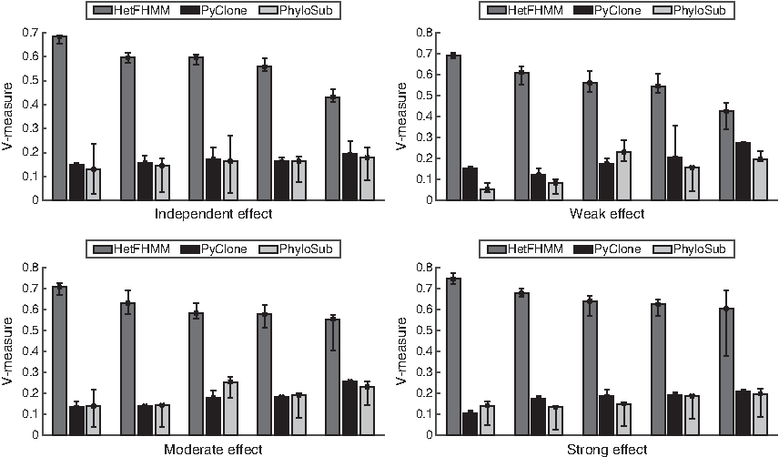
Figure 2 shows the average V–Measure results on synthetic data. It contains four plots, where each of which corresponds to the results on data containing strong, normal, weak, and no dependency between adjacent mutations. In each plot, there are five groups of results corresponding to synthetic data with a different number of gold clones \documentclass{aastex}\usepackage{amsbsy}\usepackage{amsfonts}\usepackage{amssymb}\usepackage{bm}\usepackage{mathrsfs}\usepackage{pifont}\usepackage{stmaryrd}\usepackage{textcomp}\usepackage{portland, xspace}\usepackage{amsmath, amsxtra}\usepackage{upgreek}\pagestyle{empty}\DeclareMathSizes{10}{9}{7}{6}\begin{document}
$$\{ 3 , 4 , 5 , 6 , 8 \} $$
\end{document}. Based on Figure 2, some remarks are in order. First, in all synthetic data conditions, the performance of HetFHMM is superior compared with PyClone and PhyloSub. Further investigation of the results revealed that HetFHMM detected the same number of clones as the gold standard.
Average V–Measure of the clustered outputs of HetFHMM, PyClone, and PhyloSub on synthetic data. The four panels show results on data generated with different degrees of interdependency between adjacent mutations, including strong, moderate, weak, and no interdependency. In each panel, there are multiple synthetic data, each of which corresponds to a different number of clones in \documentclass{aastex}\usepackage{amsbsy}\usepackage{amsfonts}\usepackage{amssymb}\usepackage{bm}\usepackage{mathrsfs}\usepackage{pifont}\usepackage{stmaryrd}\usepackage{textcomp}\usepackage{portland, xspace}\usepackage{amsmath, amsxtra}\usepackage{upgreek}\pagestyle{empty}\DeclareMathSizes{10}{9}{7}{6}\begin{document}
$$\{ 3 , 4 , 5 , 6 , 8 \} $$
\end{document}. For each data condition, our model (dark grey bars) is compared with PhyloSub (black bars) and PyClone (light grey bars).
However, PyClone and PhyloSub detected many more clusters than the gold standard, which in turn affected their average V–Measure scores. Second, as interdependency between adjacent mutations becomes stronger, the performance of HetFHMM improves. This is in contrast to the performances of PyClone and PhyloSub that do not change as adjacent mutations influence changes. This is due to the fact that HetFHMM models the dependency between adjacent mutations through the value of \documentclass{aastex}\usepackage{amsbsy}\usepackage{amsfonts}\usepackage{amssymb}\usepackage{bm}\usepackage{mathrsfs}\usepackage{pifont}\usepackage{stmaryrd}\usepackage{textcomp}\usepackage{portland, xspace}\usepackage{amsmath, amsxtra}\usepackage{upgreek}\pagestyle{empty}\DeclareMathSizes{10}{9}{7}{6}\begin{document}
$$\rho$$
\end{document} in the transition probability [Eqn. (2)]. Hence, in the data including strongly influenced adjacent mutations, \documentclass{aastex}\usepackage{amsbsy}\usepackage{amsfonts}\usepackage{amssymb}\usepackage{bm}\usepackage{mathrsfs}\usepackage{pifont}\usepackage{stmaryrd}\usepackage{textcomp}\usepackage{portland, xspace}\usepackage{amsmath, amsxtra}\usepackage{upgreek}\pagestyle{empty}\DeclareMathSizes{10}{9}{7}{6}\begin{document}
$$\rho$$
\end{document} helps to predict the genotype of a mutation more accurately compared with the data containing weaker influence between adjacent mutations. On the other hand, PyClone and PhyloSub do not take into account the dependency between adjacent mutations, hence their performances do not change as the strength of the influence changes. Third, the accuracy of cluster identification of HetFHMM decreases as the number of clones increases. This is in contrast to PyClone and PhyloSub that showed little improvement when the number of clones is increased (but still significantly outperformed by HetFHMM).
In Section 4, we have mentioned that a special type of synthetic data is generated where mutations do not have influences among themselves, which is the assumption made in PyClone and PhyloSub. Based on Figure 2, it is interesting to see that HetFHMM performs better than PyClone and PhyloSub even on this data condition. It indicates that HetFHMM can work better than the baselines no matter whether there is interdependency between adjacent mutations.
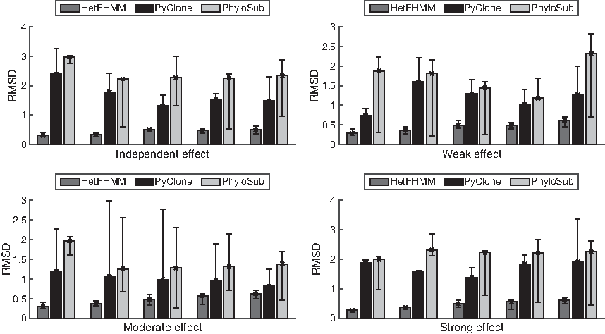
In addition to V–Measure to evaluate the cluster output, we have evaluated the cellular prevalence predicted by HetFHMM, PyClone, and PhyloSub using the RMSD score. Figure 3 presents the average RMSD errors for our model and the baselines on all synthetic data conditions. We see the similar trend that HetFHMM outperforms the baseline models on all data conditions. This is, in part, due to the more correctly predicted clones by HetFHMM.
Average root mean-square distance of the clustered outputs of HetFHMM, PyClone, and PhyloSub on synthetic data. The four panels show results on data generated with different degrees of interdependency between adjacent mutations, including strong, moderate, weak, and no interdependency. In each panel, there are multiple synthetic data, each of which corresponds to a different number of clones in \documentclass{aastex}\usepackage{amsbsy}\usepackage{amsfonts}\usepackage{amssymb}\usepackage{bm}\usepackage{mathrsfs}\usepackage{pifont}\usepackage{stmaryrd}\usepackage{textcomp}\usepackage{portland, xspace}\usepackage{amsmath, amsxtra}\usepackage{upgreek}\pagestyle{empty}\DeclareMathSizes{10}{9}{7}{6}\begin{document}
$$\{ 3 , 4 , 5 , 6 , 8 \} $$
\end{document}. For each data condition, our model (dark grey bars) is compared with PhyloSub (black bars) and PyClone (light grey bars).
5.2. Real cancer data
We apply our model to Ding et al.'s (2012) AML (described in Subsection 4.1) data, which is annotated with gold clones based on laboratory experiments. However, it is not annotated with the cellular prevalence of clones; therefore, we can only use V–Measure to test the quality of predicted clones as RMSD is not applicable. For HetFHMM, we run the model with a different number of clones, from 3 to 10, and choose the one with the highest log likelihood.
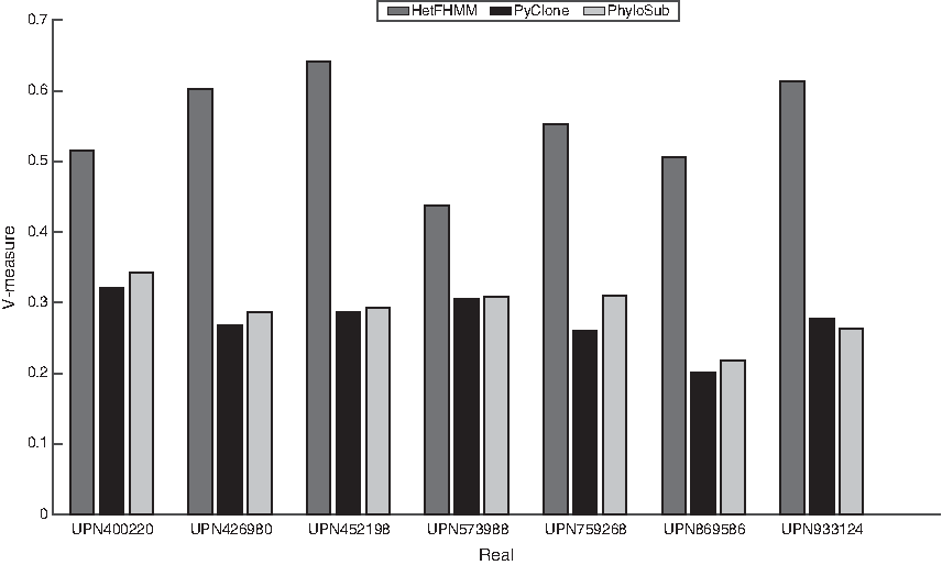
Figure 4 shows the V–Measure scores as per patient sample. Based on the results, it is clear that HetFHMM has predicted the clusters more accurately than PyClone and PhyloSub for all patients. The accuracy of PyClone and PhyloSub has been almost the same for all cases, except patients UPN869586 and UPN933124, where PhyloSub detected more accurate clones compared with PyClone.
V–Measure of the cluster output of HetFHMM (dark grey bars), PyClone (black bars), and PhyloSub (light grey bars) on real cancer data from different acute myeloid leukemia patients.
6. Conclusion
We have developed a novel model, called HetFHMM, to identify the clonal architecture of a tumor sample based on NGS data. Our model discovers mutations as well as the cellular prevalence of clones in the sample. HetFHMM is based on FHMMs, whereby the genomic composition of each clone is represented by a hidden chain. The basis of the model is that the observed data are generated by a mixture of underlying chains, where the mixing coefficients are the clonal prevalence. We make use of Gibbs sampling and EG algorithms to infer clonal genomic compositions represented by the hidden chains as well as the clonal prevalence. The empirical results on synthetic and real cancer data confirm that our model outperforms strong baseline models, PhyloSub and PyClone, based on two evaluation metrics, that is, V–Measure and RMSD. The key to the stronger performance of HetFHMM compared with baseline models is that it jointly infers the clone-specific mutations and cellular prevalence to identify the tumor clones.
There are many directions for future work. First, HetFHMM is designed for single-sample cancer data; however, we envision a multiple-sample extension to further improve the quality of its results. Multiple-sample cancer data can cover spatial and temporal dimensions, where samples are obtained from different tumor regions or time points from the same patient. Second, it would be interesting to infer the number of clones using nonparametric Bayesian models, such as infinite FHMMs. Finally, we hope that research in this area results in better understanding of cancer heterogeneity that in turn can lead to better patient care and therapeutic strategies.
Substitute \documentclass{aastex}\usepackage{amsbsy}\usepackage{amsfonts}\usepackage{amssymb}\usepackage{bm}\usepackage{mathrsfs}\usepackage{pifont}\usepackage{stmaryrd}\usepackage{textcomp}\usepackage{portland, xspace}\usepackage{amsmath, amsxtra}\usepackage{upgreek}\pagestyle{empty}\DeclareMathSizes{10}{9}{7}{6}\begin{document}
$$ { \frac { d { P_ { { b_t } } } } { d { \phi _k } } } $$
\end{document} and \documentclass{aastex}\usepackage{amsbsy}\usepackage{amsfonts}\usepackage{amssymb}\usepackage{bm}\usepackage{mathrsfs}\usepackage{pifont}\usepackage{stmaryrd}\usepackage{textcomp}\usepackage{portland, xspace}\usepackage{amsmath, amsxtra}\usepackage{upgreek}\pagestyle{empty}\DeclareMathSizes{10}{9}{7}{6}\begin{document}
$$ { \frac { d { \mu _t } } { d { \phi _k } } } $$
\end{document} back to \documentclass{aastex}\usepackage{amsbsy}\usepackage{amsfonts}\usepackage{amssymb}\usepackage{bm}\usepackage{mathrsfs}\usepackage{pifont}\usepackage{stmaryrd}\usepackage{textcomp}\usepackage{portland, xspace}\usepackage{amsmath, amsxtra}\usepackage{upgreek}\pagestyle{empty}\DeclareMathSizes{10}{9}{7}{6}\begin{document}
$$\mathcal{L} ( \Phi )$$
\end{document}, the gradient of the objective function can be found with respect to variable \documentclass{aastex}\usepackage{amsbsy}\usepackage{amsfonts}\usepackage{amssymb}\usepackage{bm}\usepackage{mathrsfs}\usepackage{pifont}\usepackage{stmaryrd}\usepackage{textcomp}\usepackage{portland, xspace}\usepackage{amsmath, amsxtra}\usepackage{upgreek}\pagestyle{empty}\DeclareMathSizes{10}{9}{7}{6}\begin{document}
$$\Phi$$
\end{document}.
7.2. Appendix B: Evaluation measures
HetFHMM produces two types of outputs: mutations forming clusters/clones and proportion of clusters/clones. These outputs are evaluated by two evaluation measures: V–Measure and RMSD, respectively.
7.2.1. V–Measure
Rosenberg and Hirschberg (2007) introduced this measure to quantify the quality of a predicted clustering with respect to the gold standard. It is an entropy-based measure that is a function of the completeness‡ and homogeneity§ of predicted clusters with respect to the gold standard. The notion of homogeneity is defined as follows:
\documentclass{aastex}\usepackage{amsbsy}\usepackage{amsfonts}\usepackage{amssymb}\usepackage{bm}\usepackage{mathrsfs}\usepackage{pifont}\usepackage{stmaryrd}\usepackage{textcomp}\usepackage{portland, xspace}\usepackage{amsmath, amsxtra}\usepackage{upgreek}\pagestyle{empty}\DeclareMathSizes{10}{9}{7}{6}\begin{document}
\begin{align*}
h = \left\{ { \begin{matrix} 1 \hfill & {{ \rm{if}}} \hfill & {H{ \rm{ ( }}G{ \rm{ \vert }}P{ \rm{ ) }} \ { \rm{ = }} \ { \rm{0}}} \hfill \\ {1 - {{H ( G \vert P ) } \over {H ( G ) }}} \hfill & {{ \rm{else}}} \hfill & {} \hfill \\ \end{matrix} } \right. \tag{16}
\end{align*}
\end{document}
where
\documentclass{aastex}\usepackage{amsbsy}\usepackage{amsfonts}\usepackage{amssymb}\usepackage{bm}\usepackage{mathrsfs}\usepackage{pifont}\usepackage{stmaryrd}\usepackage{textcomp}\usepackage{portland, xspace}\usepackage{amsmath, amsxtra}\usepackage{upgreek}\pagestyle{empty}\DeclareMathSizes{10}{9}{7}{6}\begin{document}
\begin{align*}
H ( G \vert P ) = - \sum \limits_ { i = 1 } ^K \sum \limits_ { j = 1 } ^C \frac { { { a_ { ji } } } } { T } \log { \frac { { a_ { ji } } } { \sum \nolimits_ { k = 1 } ^C { { a_ { ki } } } } }
\end{align*}
\end{document}
and
\documentclass{aastex}\usepackage{amsbsy}\usepackage{amsfonts}\usepackage{amssymb}\usepackage{bm}\usepackage{mathrsfs}\usepackage{pifont}\usepackage{stmaryrd}\usepackage{textcomp}\usepackage{portland, xspace}\usepackage{amsmath, amsxtra}\usepackage{upgreek}\pagestyle{empty}\DeclareMathSizes{10}{9}{7}{6}\begin{document}
\begin{align*}
H ( G ) = - \sum \limits_ { i = 1 } ^C \frac { { \sum \nolimits_ { j = 1 } ^K { { a_ { ij } } } } } { K } \log \frac { { \sum \nolimits_ { k = 1 } ^K { { a_ { ik } } } } } { K }
\end{align*}
\end{document}
G, P, C, K, T, and \documentclass{aastex}\usepackage{amsbsy}\usepackage{amsfonts}\usepackage{amssymb}\usepackage{bm}\usepackage{mathrsfs}\usepackage{pifont}\usepackage{stmaryrd}\usepackage{textcomp}\usepackage{portland, xspace}\usepackage{amsmath, amsxtra}\usepackage{upgreek}\pagestyle{empty}\DeclareMathSizes{10}{9}{7}{6}\begin{document}
$${a_{c , k}}$$
\end{document} are the set of gold standard clusters, the set of predicted clusters, the number of gold standard clusters, the number of predicted clusters, the size of a gold cluster c, and the size of the predicted cluster k. The notion of completeness is defined as follows:
\documentclass{aastex}\usepackage{amsbsy}\usepackage{amsfonts}\usepackage{amssymb}\usepackage{bm}\usepackage{mathrsfs}\usepackage{pifont}\usepackage{stmaryrd}\usepackage{textcomp}\usepackage{portland, xspace}\usepackage{amsmath, amsxtra}\usepackage{upgreek}\pagestyle{empty}\DeclareMathSizes{10}{9}{7}{6}\begin{document}
\begin{align*}
c = \left\{ { \begin{matrix} 1 \hfill & {{ \rm{if}}} \hfill & {H{ \rm{ ( }}P{ \rm{ \vert }}G{ \rm{ ) }} \ { \rm{ = }} \ { \rm{0}}} \hfill \\ {1 - {{H ( P \vert G ) } \over {H ( P ) }}} \hfill & {{ \rm{else}}} \hfill & {} \hfill \\ \end{matrix} } \right. \tag{17}
\end{align*}
\end{document}
where
\documentclass{aastex}\usepackage{amsbsy}\usepackage{amsfonts}\usepackage{amssymb}\usepackage{bm}\usepackage{mathrsfs}\usepackage{pifont}\usepackage{stmaryrd}\usepackage{textcomp}\usepackage{portland, xspace}\usepackage{amsmath, amsxtra}\usepackage{upgreek}\pagestyle{empty}\DeclareMathSizes{10}{9}{7}{6}\begin{document}
\begin{align*}
H ( P \vert G ) = - \sum \limits_ { i = 1 } ^C \sum \limits_ { j = 1 } ^K \frac { { { a_ { ij } } } } { T } \log { \frac { { a_ { ij } } } { \sum \nolimits_ { k = 1 } ^K { { a_ { ik } } } } }
\end{align*}
\end{document}\documentclass{aastex}\usepackage{amsbsy}\usepackage{amsfonts}\usepackage{amssymb}\usepackage{bm}\usepackage{mathrsfs}\usepackage{pifont}\usepackage{stmaryrd}\usepackage{textcomp}\usepackage{portland, xspace}\usepackage{amsmath, amsxtra}\usepackage{upgreek}\pagestyle{empty}\DeclareMathSizes{10}{9}{7}{6}\begin{document}
\begin{align*}
H ( P ) = - \sum \limits_ { i = 1 } ^K \frac { { \sum \nolimits_ { j = 1 } ^C { { a_ { ji } } } } } { C } \log \frac { { \sum \nolimits_ { k = 1 } ^C { { a_ { ki } } } } } { C }
\end{align*}
\end{document}
\documentclass{aastex}\usepackage{amsbsy}\usepackage{amsfonts}\usepackage{amssymb}\usepackage{bm}\usepackage{mathrsfs}\usepackage{pifont}\usepackage{stmaryrd}\usepackage{textcomp}\usepackage{portland, xspace}\usepackage{amsmath, amsxtra}\usepackage{upgreek}\pagestyle{empty}\DeclareMathSizes{10}{9}{7}{6}\begin{document}
$$H ( G \vert P )$$
\end{document} and \documentclass{aastex}\usepackage{amsbsy}\usepackage{amsfonts}\usepackage{amssymb}\usepackage{bm}\usepackage{mathrsfs}\usepackage{pifont}\usepackage{stmaryrd}\usepackage{textcomp}\usepackage{portland, xspace}\usepackage{amsmath, amsxtra}\usepackage{upgreek}\pagestyle{empty}\DeclareMathSizes{10}{9}{7}{6}\begin{document}
$$H ( ( P \vert G )$$
\end{document} compute the nonhomogeneity and incompleteness of the output clustering, respectively. When \documentclass{aastex}\usepackage{amsbsy}\usepackage{amsfonts}\usepackage{amssymb}\usepackage{bm}\usepackage{mathrsfs}\usepackage{pifont}\usepackage{stmaryrd}\usepackage{textcomp}\usepackage{portland, xspace}\usepackage{amsmath, amsxtra}\usepackage{upgreek}\pagestyle{empty}\DeclareMathSizes{10}{9}{7}{6}\begin{document}
$$H ( G \vert P )$$
\end{document} or \documentclass{aastex}\usepackage{amsbsy}\usepackage{amsfonts}\usepackage{amssymb}\usepackage{bm}\usepackage{mathrsfs}\usepackage{pifont}\usepackage{stmaryrd}\usepackage{textcomp}\usepackage{portland, xspace}\usepackage{amsmath, amsxtra}\usepackage{upgreek}\pagestyle{empty}\DeclareMathSizes{10}{9}{7}{6}\begin{document}
$$H ( P \vert G )$$
\end{document} is zero, the output clustering is either homogeneous or complete to the gold standard clone. When the value of \documentclass{aastex}\usepackage{amsbsy}\usepackage{amsfonts}\usepackage{amssymb}\usepackage{bm}\usepackage{mathrsfs}\usepackage{pifont}\usepackage{stmaryrd}\usepackage{textcomp}\usepackage{portland, xspace}\usepackage{amsmath, amsxtra}\usepackage{upgreek}\pagestyle{empty}\DeclareMathSizes{10}{9}{7}{6}\begin{document}
$$H ( G \vert P )$$
\end{document} or \documentclass{aastex}\usepackage{amsbsy}\usepackage{amsfonts}\usepackage{amssymb}\usepackage{bm}\usepackage{mathrsfs}\usepackage{pifont}\usepackage{stmaryrd}\usepackage{textcomp}\usepackage{portland, xspace}\usepackage{amsmath, amsxtra}\usepackage{upgreek}\pagestyle{empty}\DeclareMathSizes{10}{9}{7}{6}\begin{document}
$$H ( P \vert G )$$
\end{document} is other than zero, the degree of nonhomogeneity or incompleteness is computed by \documentclass{aastex}\usepackage{amsbsy}\usepackage{amsfonts}\usepackage{amssymb}\usepackage{bm}\usepackage{mathrsfs}\usepackage{pifont}\usepackage{stmaryrd}\usepackage{textcomp}\usepackage{portland, xspace}\usepackage{amsmath, amsxtra}\usepackage{upgreek}\pagestyle{empty}\DeclareMathSizes{10}{9}{7}{6}\begin{document}
$$ { \frac { H ( G \vert P ) } { H ( G ) } } $$
\end{document} or \documentclass{aastex}\usepackage{amsbsy}\usepackage{amsfonts}\usepackage{amssymb}\usepackage{bm}\usepackage{mathrsfs}\usepackage{pifont}\usepackage{stmaryrd}\usepackage{textcomp}\usepackage{portland, xspace}\usepackage{amsmath, amsxtra}\usepackage{upgreek}\pagestyle{empty}\DeclareMathSizes{10}{9}{7}{6}\begin{document}
$$ { \frac { H ( P \vert G ) } { H ( P ) } } $$
\end{document}, respectively.
V–Measure is then defined as the harmonic mean of the homogeneity and completeness scores:
\documentclass{aastex}\usepackage{amsbsy}\usepackage{amsfonts}\usepackage{amssymb}\usepackage{bm}\usepackage{mathrsfs}\usepackage{pifont}\usepackage{stmaryrd}\usepackage{textcomp}\usepackage{portland, xspace}\usepackage{amsmath, amsxtra}\usepackage{upgreek}\pagestyle{empty}\DeclareMathSizes{10}{9}{7}{6}\begin{document}
\begin{align*}
V { \kern 1pt } - { \kern 1pt } measure = { \frac { 2hc } { h + c } } \tag { 18 }
\end{align*}
\end{document}
For prefect clustering, the score would be one, and it is less than one for any imperfect clustering. For clustering far away from the gold, the V–Measure would be smaller than one and gets closer to zero.
7.2.1. Root mean-square distance
We evaluate the predicted cellular prevalence with respect to the gold standard using root mean-square distance or RMSD. It is used to compute the distance or gap between the cellular prevalence of predicted clusters and the gold standard:
\documentclass{aastex}\usepackage{amsbsy}\usepackage{amsfonts}\usepackage{amssymb}\usepackage{bm}\usepackage{mathrsfs}\usepackage{pifont}\usepackage{stmaryrd}\usepackage{textcomp}\usepackage{portland, xspace}\usepackage{amsmath, amsxtra}\usepackage{upgreek}\pagestyle{empty}\DeclareMathSizes{10}{9}{7}{6}\begin{document}
\begin{align*}
RMSD = \sqrt{ \frac {{1}} {{ | S | }}\sum \limits_ {\forall \bar
S } || { \Phi _n } - { \Phi _N } { || ^2 } + \frac { 1 } { { \bar
| S | } } \sum \limits_ { \forall \bar S } || { \Phi _n } - 0 { ||
^2 }} \tag { 19 }
\end{align*}
\end{document}
where S and \documentclass{aastex}\usepackage{amsbsy}\usepackage{amsfonts}\usepackage{amssymb}\usepackage{bm}\usepackage{mathrsfs}\usepackage{pifont}\usepackage{stmaryrd}\usepackage{textcomp}\usepackage{portland, xspace}\usepackage{amsmath, amsxtra}\usepackage{upgreek}\pagestyle{empty}\DeclareMathSizes{10}{9}{7}{6}\begin{document}
$$\bar S$$
\end{document} are significant and insignificant predicted clusters, respectively. Most methods produce more clusters than the gold standard. Among the predicted clusters, the ones containing a larger number of mutations in common with the gold standard are known as significant clusters. The remaining clusters are known as insignificant clusters. The better the quality of the predicted clones and their prevalence, the lower would be the RMSD.
Footnotes
Acknowledgment
The authors are thankful to Monash University for the financial support towards this research.
Author Disclosure Statement
No competing financial interests exist.
References
1.
CaracoY.1998. Genetic determinants of drug responsiveness and drug interactions. J. Ther. Drug Monit., 20, 517–524.
2.
ColellaS., YauC., TaylorJ. M., et al.2007. QuantiSNP: An objective bayes hidden-markov model to detect and accurately map copy number variation using SNP genotyping data. Nucleic Acid Res. 35, 2013–2025.
3.
DeshwarA.G., VembuS., YungC.K., et al.2015. Phylowgs: Reconstructing subclonal composition and evolution from whole-genome sequencing of tumors. Genome Biol. 15, 1–10.
4.
DingL., LeyT.J., LarsonD.E., et al.2012. Clonal evolution in relapsed acute myeloid leukaemia revealed by whole-genome sequencing. Nature. 481, 506–512.
5.
GhahramaniZ., and JordanM.I.1997. Factorial hidden markov models. J. Mach. Learn. 29, 245–273.
6.
HaG., RothA., LaiD., et al.2012. Integrative analysis of genome-wide loss of heterozygosity and monoallelic expression at nucleotide resolution reveals disrupted pathways in triple-negative breast cancer. Genome Res. 20, 1995–2007.
7.
HajirasoulihaI., MahmoodyA., and RaphaelB.J.2014. A combinatorial approach for analyzing intra-tumour heterogeneity from high-throughput sequencing data. Oxford J Bioinformat. 30, i78–i86.
8.
JiaoW., VembuS., DeshwarA.G., et al.2014. Inferring clonal evolution of tumours from single nucleotide somatic mutations. BMC Bioinformat. 15, 1–16.
9.
LiA., LiuZ., Lezon-GeydaK., et al.2011. GPHMM: An integrated hidden markov model for identification of copy number alteration and loss of heterozygosity in complex tumour samples using whole genome SNP arrays. Nucleic Acids Res. 39, 4928–4941.
10.
MalikicS., McPhersonA., DonmezN., et al.2015. Clonality inference in multiple tumor samples using phylogeny. Oxford J. Bioinformat. 31, 1349–1356.
11.
RosenbergA., and HirschbergJ.B.2007. V-measure: A conditional entropy-based external cluster evaluation. Proceedings of the 2007 Joint Conference on Empirical Methods in Natural Language Processing and Computational Natural Language Learning (EMNLP-CoNLL), pp. 410–420.
12.
RothA., KhattraJ., YapD., et al.2014. PyClone: Statistical inference of clonal population structure in cancer. Nat. Methods. 11, 396–398.
13.
StrattonM.R., CampbellP.J., and FutrealP.A.2009. The cancer genome. Nature. 458, 719–724.
14.
XiaH., LiuY., WangM., et al.2013. A novel HMM for analyzing chromosomal aberrations in heterogeneous tumour samples. Proceedings of the 7th International Conference on Systems Biology (ISB), pp. 92–96.
15.
YauC.2013. OncoSNP-seq: A statistical approach for the identification of somatic copy number alternations from next generation sequencing of cancer genomes. Oxford J. Bioinformat. 29, 2482–2484.