In modeling censored data, survival forest models are a competitive nonparametric alternative to traditional parametric or semiparametric models when the function forms are possibly misspecified or the underlying assumptions are violated. In this work, we propose a survival forest approach with trees constructed using a novel pseudo R2 splitting rules. By studying the well-known benchmark data sets, we find that the proposed model generally outperforms popular survival models such as random survival forest with different splitting rules, Cox proportional hazard model, and generalized boosted model in terms of C-index metric.
1. Introduction
In the field of medical and biological research, censored survival data are often studied using (semi-)parametric models such as Cox proportional hazard models (David, 1972) and accelerated failure time models (Cai et al., 2009). However, the underlying assumptions to these models are not easily satisfied in practice. In this case, nonparametric survival trees and survival forests, which have the inherent advantage of determining the relationship between covariates and hazard in censored data, are useful alternatives (Gordon and Olshen, 1985; Ishwaran et al., 2008; Zhu and Kosorok, 2012; Steingrimsson et al., 2016).
In general, the construction of a survival decision tree involves two major steps: the tree growing step and the tree pruning step (Cappelli and Zhang, 2007). The choice of splitting functions in the growing step is usually crucial to the performance of decision trees (Mbogning and Broët, 2016). Owing to the presence of censored data, splitting functions developed for classification and regression problems such as information gain, Gini index, and mean squared error (Breiman et al., 1984) are not appropriate in the context of survival analysis. To deal with this problem, various splitting functions for survival data have been proposed and generally they can be categorized into two types: maximization of between-node heterogeneity and minimization of within-node homogeneity. These splitting functions are based on various statistics or quantities such as the L1-Wasserstein distance between the Kaplan–Meier estimators of two child nodes (Gordon and Olshen, 1985), log-rank test statistic (Ciampi et al., 1986; LeBlanc and Crowley, 1993), likelihood ratio statistic (Ciampi et al., 1987), Wilcoxon–Gehan statistics (Ciampi et al., 1989), two-sample Tarone–Ware statistics (Segal, 1988), L1 loss function (Cho and Hong, 2008), and C-index statistic (Schmid et al., 2016). And among them, the most popular splitting rule is the log-rank test statistic. A review on various splitting functions can be found in Bou-Hamad et al. (2011) and comparative studies of common splitting criteria have been performed by Shimokawa et al. (2015, 2016).
A single survival tree, however, can be potentially unstable as it is very sensitive to small changes in the data. This problem is usually mitigated by using a variety of ensemble methods such as survival bagging (Hothorn et al., 2004, 2006; Mbogning and Broët, 2016), or random survival forest (RSF) (Ishwaran et al., 2008; Wright and Ziegler, 2017). Among them, the most popular and widely applied survival ensemble is RSF, which extends random forest (Breiman, 2001) from classification and regression scenarios to survival analysis. In this method, tree node splits are designed to maximizing survival differences between subtree nodes. A so-called ensemble cumulative hazard function (CHF) can be obtained by aggregating Nelson-Aalen estimators for all “in-bag” data. Similar to survival trees, in most implementations of RSFs, the best split of a node is usually judged by the log-rank test statistic (Pang et al., 2010).
From the aforementioned studies, one may observe that the log-rank test can be regarded as the de facto splitting criterion is survival trees and survival forests. However, the log-rank test is most powerful when the true hazard curve is proportional to the hypothesized curve (Bathke et al., 2009). And in the case of crossed Kaplan–Meier survival curves (i.e., nonproportional hazards), which is not uncommon in medical practice, this test statistic could be problematic. Consequently, survival trees or forests based on this kind of splitting functions may not be adequate.
Thus, different from previous log-rank-based splitting functions, we propose and investigate a splitting rule based on a newly proposed R2 prediction measure (Li and Wang, 2016) for a nonlinear model and for right-censored survival data. The major reasons why we want to use the R2 statistic instead of other similar measures for tree nodes splitting are threefold. First, this statistic reduces to the classical coefficient of determination when no censoring is present. Second, this statistic is a consistent estimate of the nonparametric coefficient of determination when the prediction is the conditional mean response based on a correctly specified model. Third, the R2 statistic is applicable to a wide variety of event time models with right-censored data and there is no requirement for the model to be correctly specified (Li and Wang, 2016).
The rest of the article is organized as follows. Section 2 describes the preliminaries and the proposed R-squared survival forest with splitting functions based on the R2 statistic. In Section 3, the performance of R-squared survival forest is illustrated through analyzing real well-known benchmark data sets. Section 4 concludes the article and provides further research directions.
2. Methods
In this section, we first give a short introduction of survival trees and then we describe a tree splitting function based on the R2 statistic. Later on, we shall develop an ensemble of R-squared survival trees within the RSF framework.
2.1. Survival trees
A survival tree is a hierarchical model composed of discriminant functions, or splitting rules, that are applied recursively to partition the covariate space of a data set into pure covariate subspaces (Gordon and Olshen, 1985). As stated earlier, training of a survival tree involves two main steps: the growing step and the pruning step.
In the growing step, at each internal node, a certain splitting function is used to evaluate and compare all possible partition values for all covariates. The best partition value that maximizes between-node heterogeneity or minimizes within-node homogeneity is selected to split the samples at the current node into two child nodes. This process continues until some stopping conditions, such as the node samples are homogeneous or a minimum sample count is reached, are met.
In the pruning step, the algorithm removes the overfitting decision rules based on the prediction errors on an independent validation data. When related decision rules are removed, the associated internal nodes are replaced with leaf nodes. A smaller and more accurate tree is thereby obtained and the complexity of the tree model is reduced.
As stated in Breiman (2001) and Ishwaran et al. (2008), trees in random forest and RSF are usually grown without pruning. Thus, in this article, we only focus on the growing step wherein tree nodes are split recursively according to a certain splitting rule.
2.2. A splitting rule based on the R2 statistic
Assume we have a censored survival data set of size n. Denote the true survival time by a continuous random variable Y and the censoring time by a continuous variable C. However, the observed time \documentclass{aastex}\usepackage{amsbsy}\usepackage{amsfonts}\usepackage{amssymb}\usepackage{bm}\usepackage{mathrsfs}\usepackage{pifont}\usepackage{stmaryrd}\usepackage{textcomp}\usepackage{portland, xspace}\usepackage{amsmath, amsxtra}\usepackage{upgreek}\pagestyle{empty}\DeclareMathSizes{10}{9}{7}{6}\begin{document}
$$\tau$$
\end{document} is usually not fully observed, \documentclass{aastex}\usepackage{amsbsy}\usepackage{amsfonts}\usepackage{amssymb}\usepackage{bm}\usepackage{mathrsfs}\usepackage{pifont}\usepackage{stmaryrd}\usepackage{textcomp}\usepackage{portland, xspace}\usepackage{amsmath, amsxtra}\usepackage{upgreek}\pagestyle{empty}\DeclareMathSizes{10}{9}{7}{6}\begin{document}
$$\tau = min ( Y , C )$$
\end{document}. \documentclass{aastex}\usepackage{amsbsy}\usepackage{amsfonts}\usepackage{amssymb}\usepackage{bm}\usepackage{mathrsfs}\usepackage{pifont}\usepackage{stmaryrd}\usepackage{textcomp}\usepackage{portland, xspace}\usepackage{amsmath, amsxtra}\usepackage{upgreek}\pagestyle{empty}\DeclareMathSizes{10}{9}{7}{6}\begin{document}
$$\delta = I ( Y \le C )$$
\end{document} is the censoring indicator, where \documentclass{aastex}\usepackage{amsbsy}\usepackage{amsfonts}\usepackage{amssymb}\usepackage{bm}\usepackage{mathrsfs}\usepackage{pifont}\usepackage{stmaryrd}\usepackage{textcomp}\usepackage{portland, xspace}\usepackage{amsmath, amsxtra}\usepackage{upgreek}\pagestyle{empty}\DeclareMathSizes{10}{9}{7}{6}\begin{document}
$$\delta = 1$$
\end{document} represents the observation is an event and \documentclass{aastex}\usepackage{amsbsy}\usepackage{amsfonts}\usepackage{amssymb}\usepackage{bm}\usepackage{mathrsfs}\usepackage{pifont}\usepackage{stmaryrd}\usepackage{textcomp}\usepackage{portland, xspace}\usepackage{amsmath, amsxtra}\usepackage{upgreek}\pagestyle{empty}\DeclareMathSizes{10}{9}{7}{6}\begin{document}
$$\delta = 0$$
\end{document} represents the observation is censored. Let \documentclass{aastex}\usepackage{amsbsy}\usepackage{amsfonts}\usepackage{amssymb}\usepackage{bm}\usepackage{mathrsfs}\usepackage{pifont}\usepackage{stmaryrd}\usepackage{textcomp}\usepackage{portland, xspace}\usepackage{amsmath, amsxtra}\usepackage{upgreek}\pagestyle{empty}\DeclareMathSizes{10}{9}{7}{6}\begin{document}
$${ \bf{X}} = ( {X_1} , {X_2} , \cdots , {X_p} )$$
\end{document} denote a p-dimensional covariate vector and D be the data set containing n independent and identically distributed observations sampled from \documentclass{aastex}\usepackage{amsbsy}\usepackage{amsfonts}\usepackage{amssymb}\usepackage{bm}\usepackage{mathrsfs}\usepackage{pifont}\usepackage{stmaryrd}\usepackage{textcomp}\usepackage{portland, xspace}\usepackage{amsmath, amsxtra}\usepackage{upgreek}\pagestyle{empty}\DeclareMathSizes{10}{9}{7}{6}\begin{document}
$$( { \bf{X}} , \tau , \delta )$$
\end{document}, namely \documentclass{aastex}\usepackage{amsbsy}\usepackage{amsfonts}\usepackage{amssymb}\usepackage{bm}\usepackage{mathrsfs}\usepackage{pifont}\usepackage{stmaryrd}\usepackage{textcomp}\usepackage{portland, xspace}\usepackage{amsmath, amsxtra}\usepackage{upgreek}\pagestyle{empty}\DeclareMathSizes{10}{9}{7}{6}\begin{document}
$$D = ( {{ \bf{X}}_i} , { \tau _i} , { \delta _i} ) , i = 1 , 2 , \cdots , n$$
\end{document}.
The proposed algorithm partitions each internal node on the basis of the R2 statistic. Specifically, for a node t of k observations, the censoring weight is defined by
\documentclass{aastex}\usepackage{amsbsy}\usepackage{amsfonts}\usepackage{amssymb}\usepackage{bm}\usepackage{mathrsfs}\usepackage{pifont}\usepackage{stmaryrd}\usepackage{textcomp}\usepackage{portland, xspace}\usepackage{amsmath, amsxtra}\usepackage{upgreek}\pagestyle{empty}\DeclareMathSizes{10}{9}{7}{6}\begin{document}
\begin{align*}
{ w_i } = { \frac { { \frac { { \delta _i } } { \hat G ( { \tau _i } - ) } } } { \sum \nolimits_ { j = 1 } ^k { { \frac { { \delta _j } } { \hat G ( { \tau _j } - ) } } } } } , \ i = 1 , \ldots , k , \tag { 1 }
\end{align*}
\end{document}
where \documentclass{aastex}\usepackage{amsbsy}\usepackage{amsfonts}\usepackage{amssymb}\usepackage{bm}\usepackage{mathrsfs}\usepackage{pifont}\usepackage{stmaryrd}\usepackage{textcomp}\usepackage{portland, xspace}\usepackage{amsmath, amsxtra}\usepackage{upgreek}\pagestyle{empty}\DeclareMathSizes{10}{9}{7}{6}\begin{document}
$$\hat G$$
\end{document} is the Kaplan–Meier estimate (Kaplan and Meier, 1958) of \documentclass{aastex}\usepackage{amsbsy}\usepackage{amsfonts}\usepackage{amssymb}\usepackage{bm}\usepackage{mathrsfs}\usepackage{pifont}\usepackage{stmaryrd}\usepackage{textcomp}\usepackage{portland, xspace}\usepackage{amsmath, amsxtra}\usepackage{upgreek}\pagestyle{empty}\DeclareMathSizes{10}{9}{7}{6}\begin{document}
$$G ( c ) = P ( C > c )$$
\end{document}. And for a covariate Xi with a split value s, define the indicator variable by \documentclass{aastex}\usepackage{amsbsy}\usepackage{amsfonts}\usepackage{amssymb}\usepackage{bm}\usepackage{mathrsfs}\usepackage{pifont}\usepackage{stmaryrd}\usepackage{textcomp}\usepackage{portland, xspace}\usepackage{amsmath, amsxtra}\usepackage{upgreek}\pagestyle{empty}\DeclareMathSizes{10}{9}{7}{6}\begin{document}
$$X_{ij}^* ( s ) = I ( {X_{ij}} \le s ) ,$$
\end{document}\documentclass{aastex}\usepackage{amsbsy}\usepackage{amsfonts}\usepackage{amssymb}\usepackage{bm}\usepackage{mathrsfs}\usepackage{pifont}\usepackage{stmaryrd}\usepackage{textcomp}\usepackage{portland, xspace}\usepackage{amsmath, amsxtra}\usepackage{upgreek}\pagestyle{empty}\DeclareMathSizes{10}{9}{7}{6}\begin{document}
$$j = 1 , \cdots , k.$$
\end{document} Let \documentclass{aastex}\usepackage{amsbsy}\usepackage{amsfonts}\usepackage{amssymb}\usepackage{bm}\usepackage{mathrsfs}\usepackage{pifont}\usepackage{stmaryrd}\usepackage{textcomp}\usepackage{portland, xspace}\usepackage{amsmath, amsxtra}\usepackage{upgreek}\pagestyle{empty}\DeclareMathSizes{10}{9}{7}{6}\begin{document}
$${ \bar \tau ^{ ( w ) }} = \mathop \sum \limits_{j = 1}^k {w_i}{ \tau _i}$$
\end{document}. The proposed R2 splitting statistic is based on
\documentclass{aastex}\usepackage{amsbsy}\usepackage{amsfonts}\usepackage{amssymb}\usepackage{bm}\usepackage{mathrsfs}\usepackage{pifont}\usepackage{stmaryrd}\usepackage{textcomp}\usepackage{portland, xspace}\usepackage{amsmath, amsxtra}\usepackage{upgreek}\pagestyle{empty}\DeclareMathSizes{10}{9}{7}{6}\begin{document}
\begin{align*}
{ R^2 } = { \frac { \mathop \sum \limits_ { j = 1 } ^k { { w_j } { { \left\{ { m_ { \hat \theta } ^ { ( wc ) } ( X_ { ij } ^* ( s ) ) - { { \bar \tau } ^ { ( w ) } } } \right\} } ^2 } } } { \mathop \sum \limits_ { j = 1 } ^k { { w_j } { { \left\{ { { \tau _j } - { { \bar \tau } ^ { ( w ) } } } \right\} } ^2 } } } } , \tag { 2 }
\end{align*}
\end{document}
where \documentclass{aastex}\usepackage{amsbsy}\usepackage{amsfonts}\usepackage{amssymb}\usepackage{bm}\usepackage{mathrsfs}\usepackage{pifont}\usepackage{stmaryrd}\usepackage{textcomp}\usepackage{portland, xspace}\usepackage{amsmath, amsxtra}\usepackage{upgreek}\pagestyle{empty}\DeclareMathSizes{10}{9}{7}{6}\begin{document}
$$m_{ \hat \theta }^{ ( wc ) } ( X_{ij}^* ( s ) )$$
\end{document} is the fitted regression function from the weighted least squares linear regression of \documentclass{aastex}\usepackage{amsbsy}\usepackage{amsfonts}\usepackage{amssymb}\usepackage{bm}\usepackage{mathrsfs}\usepackage{pifont}\usepackage{stmaryrd}\usepackage{textcomp}\usepackage{portland, xspace}\usepackage{amsmath, amsxtra}\usepackage{upgreek}\pagestyle{empty}\DeclareMathSizes{10}{9}{7}{6}\begin{document}
$${ \tau _1} , \ldots , { \tau _k}$$
\end{document} on \documentclass{aastex}\usepackage{amsbsy}\usepackage{amsfonts}\usepackage{amssymb}\usepackage{bm}\usepackage{mathrsfs}\usepackage{pifont}\usepackage{stmaryrd}\usepackage{textcomp}\usepackage{portland, xspace}\usepackage{amsmath, amsxtra}\usepackage{upgreek}\pagestyle{empty}\DeclareMathSizes{10}{9}{7}{6}\begin{document}
$$X_{i1}^* ( s ) , \cdots X_{ik}^* ( s )$$
\end{document} with weight \documentclass{aastex}\usepackage{amsbsy}\usepackage{amsfonts}\usepackage{amssymb}\usepackage{bm}\usepackage{mathrsfs}\usepackage{pifont}\usepackage{stmaryrd}\usepackage{textcomp}\usepackage{portland, xspace}\usepackage{amsmath, amsxtra}\usepackage{upgreek}\pagestyle{empty}\DeclareMathSizes{10}{9}{7}{6}\begin{document}
$$W = diag \{ {w_1} , \ldots , {w_k} \} $$
\end{document} as defined by Li and Wang (2016). Our task is then to find the optimal splitting variable and the corresponding split point that has the largest R2 statistic from the possible binary splits defined by all available covariates at node t.
2.3. R-squared random survival forest
The proposed R-squared random survival forest (R2RSF) algorithm can be described as follows:
1. Draw \documentclass{aastex}\usepackage{amsbsy}\usepackage{amsfonts}\usepackage{amssymb}\usepackage{bm}\usepackage{mathrsfs}\usepackage{pifont}\usepackage{stmaryrd}\usepackage{textcomp}\usepackage{portland, xspace}\usepackage{amsmath, amsxtra}\usepackage{upgreek}\pagestyle{empty}\DeclareMathSizes{10}{9}{7}{6}\begin{document}
$${n_{tree}}$$
\end{document} bootstrap samples of size n from the training set D, where \documentclass{aastex}\usepackage{amsbsy}\usepackage{amsfonts}\usepackage{amssymb}\usepackage{bm}\usepackage{mathrsfs}\usepackage{pifont}\usepackage{stmaryrd}\usepackage{textcomp}\usepackage{portland, xspace}\usepackage{amsmath, amsxtra}\usepackage{upgreek}\pagestyle{empty}\DeclareMathSizes{10}{9}{7}{6}\begin{document}
$${n_{tree}}$$
\end{document} is a user-specified parameter indicating the size of a survival forest.
2. For each of the bootstrap samples, grow an unpruned R-squared survival tree such as:
(a) At each node, randomly select mtry out of p covariates as candidate split variables and mtry is usually set to \documentclass{aastex}\usepackage{amsbsy}\usepackage{amsfonts}\usepackage{amssymb}\usepackage{bm}\usepackage{mathrsfs}\usepackage{pifont}\usepackage{stmaryrd}\usepackage{textcomp}\usepackage{portland, xspace}\usepackage{amsmath, amsxtra}\usepackage{upgreek}\pagestyle{empty}\DeclareMathSizes{10}{9}{7}{6}\begin{document}
$$\sqrt p$$
\end{document}.
(b) Calculate the R2 statistic already defined for each possible split of each candidate split variable.
(c) Find the best split point and the corresponding covariate that has the maximum R2 value among all candidate splits. Then, partition the current node into two child nodes accordingly.
(d) Continue tree growing until some stopping criteria are satisfied, for example, a minimum terminal node size is reached.
(e) Calculate the hazard function of each terminal node in the tree through the Nelson-Aalen estimator. Consider a specific node h. If the training observations in the node h are represented as \documentclass{aastex}\usepackage{amsbsy}\usepackage{amsfonts}\usepackage{amssymb}\usepackage{bm}\usepackage{mathrsfs}\usepackage{pifont}\usepackage{stmaryrd}\usepackage{textcomp}\usepackage{portland, xspace}\usepackage{amsmath, amsxtra}\usepackage{upgreek}\pagestyle{empty}\DeclareMathSizes{10}{9}{7}{6}\begin{document}
$${D_h} = ( {{ \bf{X}}_i} , { \tau _i} , { \delta _i} ) , i = 1 , 2 , \ldots , {n_h}$$
\end{document}. Let \documentclass{aastex}\usepackage{amsbsy}\usepackage{amsfonts}\usepackage{amssymb}\usepackage{bm}\usepackage{mathrsfs}\usepackage{pifont}\usepackage{stmaryrd}\usepackage{textcomp}\usepackage{portland, xspace}\usepackage{amsmath, amsxtra}\usepackage{upgreek}\pagestyle{empty}\DeclareMathSizes{10}{9}{7}{6}\begin{document}
$${ \tau _{1 , h}} < { \tau _{2 , h}} < \cdots < { \tau _{{n_h} , h}}$$
\end{document} be the nh distinct event times. Then, the CHF for h is given by
\documentclass{aastex}\usepackage{amsbsy}\usepackage{amsfonts}\usepackage{amssymb}\usepackage{bm}\usepackage{mathrsfs}\usepackage{pifont}\usepackage{stmaryrd}\usepackage{textcomp}\usepackage{portland, xspace}\usepackage{amsmath, amsxtra}\usepackage{upgreek}\pagestyle{empty}\DeclareMathSizes{10}{9}{7}{6}\begin{document}
\begin{align*}
{ \hat H_h } ( \tau ) = \mathop \sum \limits_ { { \tau _ { l , h } } \le \tau } { \frac { { d_ { l , h } } } { { Y_ { l , h } } } } , \tag { 3 }
\end{align*}
\end{document}
where \documentclass{aastex}\usepackage{amsbsy}\usepackage{amsfonts}\usepackage{amssymb}\usepackage{bm}\usepackage{mathrsfs}\usepackage{pifont}\usepackage{stmaryrd}\usepackage{textcomp}\usepackage{portland, xspace}\usepackage{amsmath, amsxtra}\usepackage{upgreek}\pagestyle{empty}\DeclareMathSizes{10}{9}{7}{6}\begin{document}
$${d_{l , h}}$$
\end{document} and \documentclass{aastex}\usepackage{amsbsy}\usepackage{amsfonts}\usepackage{amssymb}\usepackage{bm}\usepackage{mathrsfs}\usepackage{pifont}\usepackage{stmaryrd}\usepackage{textcomp}\usepackage{portland, xspace}\usepackage{amsmath, amsxtra}\usepackage{upgreek}\pagestyle{empty}\DeclareMathSizes{10}{9}{7}{6}\begin{document}
$${Y_{l , h}}$$
\end{document} are the number of deaths and individuals at risk at time \documentclass{aastex}\usepackage{amsbsy}\usepackage{amsfonts}\usepackage{amssymb}\usepackage{bm}\usepackage{mathrsfs}\usepackage{pifont}\usepackage{stmaryrd}\usepackage{textcomp}\usepackage{portland, xspace}\usepackage{amsmath, amsxtra}\usepackage{upgreek}\pagestyle{empty}\DeclareMathSizes{10}{9}{7}{6}\begin{document}
$${ \tau _{l , h}}$$
\end{document}. It is obvious that all observations within the same terminal node have the same CHF.
3. Calculate an ensemble cumulative hazard estimate by combining information from all the ntree trees in the survival forest.
4. To predict the CHF of a new observation \documentclass{aastex}\usepackage{amsbsy}\usepackage{amsfonts}\usepackage{amssymb}\usepackage{bm}\usepackage{mathrsfs}\usepackage{pifont}\usepackage{stmaryrd}\usepackage{textcomp}\usepackage{portland, xspace}\usepackage{amsmath, amsxtra}\usepackage{upgreek}\pagestyle{empty}\DeclareMathSizes{10}{9}{7}{6}\begin{document}
$$\chi$$
\end{document}, we drop its covariates \documentclass{aastex}\usepackage{amsbsy}\usepackage{amsfonts}\usepackage{amssymb}\usepackage{bm}\usepackage{mathrsfs}\usepackage{pifont}\usepackage{stmaryrd}\usepackage{textcomp}\usepackage{portland, xspace}\usepackage{amsmath, amsxtra}\usepackage{upgreek}\pagestyle{empty}\DeclareMathSizes{10}{9}{7}{6}\begin{document}
$${ \chi _{new}}$$
\end{document} down each survival tree within the forest. Owing to the survival tree's binary nature, \documentclass{aastex}\usepackage{amsbsy}\usepackage{amsfonts}\usepackage{amssymb}\usepackage{bm}\usepackage{mathrsfs}\usepackage{pifont}\usepackage{stmaryrd}\usepackage{textcomp}\usepackage{portland, xspace}\usepackage{amsmath, amsxtra}\usepackage{upgreek}\pagestyle{empty}\DeclareMathSizes{10}{9}{7}{6}\begin{document}
$$\chi$$
\end{document} will fall into a unique terminal node \documentclass{aastex}\usepackage{amsbsy}\usepackage{amsfonts}\usepackage{amssymb}\usepackage{bm}\usepackage{mathrsfs}\usepackage{pifont}\usepackage{stmaryrd}\usepackage{textcomp}\usepackage{portland, xspace}\usepackage{amsmath, amsxtra}\usepackage{upgreek}\pagestyle{empty}\DeclareMathSizes{10}{9}{7}{6}\begin{document}
$${h^*}$$
\end{document} of each tree. Hence, the CHF prediction from a single tree is \documentclass{aastex}\usepackage{amsbsy}\usepackage{amsfonts}\usepackage{amssymb}\usepackage{bm}\usepackage{mathrsfs}\usepackage{pifont}\usepackage{stmaryrd}\usepackage{textcomp}\usepackage{portland, xspace}\usepackage{amsmath, amsxtra}\usepackage{upgreek}\pagestyle{empty}\DeclareMathSizes{10}{9}{7}{6}\begin{document}
$$\hat H ( \tau \vert { \chi _{new}} ) = \hat H_h^* ( \tau )$$
\end{document} and the ensemble CHF for \documentclass{aastex}\usepackage{amsbsy}\usepackage{amsfonts}\usepackage{amssymb}\usepackage{bm}\usepackage{mathrsfs}\usepackage{pifont}\usepackage{stmaryrd}\usepackage{textcomp}\usepackage{portland, xspace}\usepackage{amsmath, amsxtra}\usepackage{upgreek}\pagestyle{empty}\DeclareMathSizes{10}{9}{7}{6}\begin{document}
$$\chi$$
\end{document} is the average of all values of CHF over ntree survival trees.
3. Results and Discussion
In this section, we first describe the data sets used in the experiments and then we present the performance metrics and statistical tests we have adopted. Finally, we give and discuss the experimental results.
3.1. Data sets
To show the effectiveness of the proposed R2RSF model, we consider various benchmark data sets that have been extensively analyzed in the statistical literature. All of these 12 data sets are from respective R packages on the CRAN repository (R Core Team, 2016). These data sets include fields of study covering mainly breast cancer, lung cancer, colon cancer, squamous carcinoma, primary biliary cirrhosis, chronic myelogenous leukemia, and drug abuse. The amount of censored data for each data set varies, ranging from a lowest censoring rate of 7% to a highest rate of 86%.
Table 1 shows the characteristics of the 12 data sets used in the experiments.
Descriptions of the Data sets
Data set
Sample size
No. of covariates
Censoring rate (%)
Source R package
Burn
154
15
69
iBST
CML
507
5
21
multcomp
Colon
1776
12
51
survival
GBSG
686
8
56
mfp
Lung
167
8
28
survival
NWTCO
4028
5
86
survival
PBC
276
17
60
randomForestSRC
Pharynx
195
10
27
invGauss
Stagec
134
6
64
rpart
UIS
575
9
19
prLogistic
Veteran
137
6
7
survival
WPBC
194
32
76
TH.data
3.2. Performance metric and statistical tests
In this study, Harrell's concordance index (C-index or C-statistic) (Harrell et al., 1996) is employed to evaluate the predictive performance of a survival model for it is the most common discrimination metric in survival analysis (Ishwaran et al., 2008; McGeechan et al., 2008; Tripepi et al., 2010; Schmid et al., 2016). The C-index metric is popular as it can account for the whole range of observed survival times and is also easy to calculate and interpret (Schmid and Potapov, 2012). The C-index takes the following form:
\documentclass{aastex}\usepackage{amsbsy}\usepackage{amsfonts}\usepackage{amssymb}\usepackage{bm}\usepackage{mathrsfs}\usepackage{pifont}\usepackage{stmaryrd}\usepackage{textcomp}\usepackage{portland, xspace}\usepackage{amsmath, amsxtra}\usepackage{upgreek}\pagestyle{empty}\DeclareMathSizes{10}{9}{7}{6}\begin{document}
\begin{align*}
C - index = { \frac { \mathop \sum \limits_ { i , j \in \Omega } {
I \{ { { \hat s } _i } < { { \hat s } _j } \} + 0.5 \times I \{ {
{ \hat s } _i } = { { \hat s } _j } \} } } { \vert \Omega \vert }
} , \tag { 4 }
\end{align*}
\end{document}
where I is an indicator function and \documentclass{aastex}\usepackage{amsbsy}\usepackage{amsfonts}\usepackage{amssymb}\usepackage{bm}\usepackage{mathrsfs}\usepackage{pifont}\usepackage{stmaryrd}\usepackage{textcomp}\usepackage{portland, xspace}\usepackage{amsmath, amsxtra}\usepackage{upgreek}\pagestyle{empty}\DeclareMathSizes{10}{9}{7}{6}\begin{document}
$${ \hat s_i} , { \hat s_j}$$
\end{document} stands for the predicted survival probabilities of patients i and j, respectively. And \documentclass{aastex}\usepackage{amsbsy}\usepackage{amsfonts}\usepackage{amssymb}\usepackage{bm}\usepackage{mathrsfs}\usepackage{pifont}\usepackage{stmaryrd}\usepackage{textcomp}\usepackage{portland, xspace}\usepackage{amsmath, amsxtra}\usepackage{upgreek}\pagestyle{empty}\DeclareMathSizes{10}{9}{7}{6}\begin{document}
$$\Omega$$
\end{document} is the set of all pairs of patients \documentclass{aastex}\usepackage{amsbsy}\usepackage{amsfonts}\usepackage{amssymb}\usepackage{bm}\usepackage{mathrsfs}\usepackage{pifont}\usepackage{stmaryrd}\usepackage{textcomp}\usepackage{portland, xspace}\usepackage{amsmath, amsxtra}\usepackage{upgreek}\pagestyle{empty}\DeclareMathSizes{10}{9}{7}{6}\begin{document}
$$\{ i , j \} $$
\end{document} who satisfy one of the following conditions: (a) both patients experienced an event and the corresponding true survival times \documentclass{aastex}\usepackage{amsbsy}\usepackage{amsfonts}\usepackage{amssymb}\usepackage{bm}\usepackage{mathrsfs}\usepackage{pifont}\usepackage{stmaryrd}\usepackage{textcomp}\usepackage{portland, xspace}\usepackage{amsmath, amsxtra}\usepackage{upgreek}\pagestyle{empty}\DeclareMathSizes{10}{9}{7}{6}\begin{document}
$${ \tau _i} < { \tau _j}$$
\end{document} and in case \documentclass{aastex}\usepackage{amsbsy}\usepackage{amsfonts}\usepackage{amssymb}\usepackage{bm}\usepackage{mathrsfs}\usepackage{pifont}\usepackage{stmaryrd}\usepackage{textcomp}\usepackage{portland, xspace}\usepackage{amsmath, amsxtra}\usepackage{upgreek}\pagestyle{empty}\DeclareMathSizes{10}{9}{7}{6}\begin{document}
$${ \tau _i} = { \tau _j}$$
\end{document} we count it as an half pair; (b) only patient i experienced an event and \documentclass{aastex}\usepackage{amsbsy}\usepackage{amsfonts}\usepackage{amssymb}\usepackage{bm}\usepackage{mathrsfs}\usepackage{pifont}\usepackage{stmaryrd}\usepackage{textcomp}\usepackage{portland, xspace}\usepackage{amsmath, amsxtra}\usepackage{upgreek}\pagestyle{empty}\DeclareMathSizes{10}{9}{7}{6}\begin{document}
$${ \tau _i} < { \tau _j}$$
\end{document}.
Note that C-index = 1 indicates the model has a perfect prediction, and C-index = 0.5 implies that the model is as good as a random predictor. Usually, a larger C-index implies a better performance of the model.
To test whether a model performs significantly better than other models, we use two types of statistic tests: the nonparametric Friedman test and the Nemenyi post hoc test (Demšar, 2006). If the p-value of the Friedman test is less than a threshold (say, 0.05), the null hypothesis that there is no significant difference among the compared survival models can be rejected and a Nemenyi post hoc test can be adopted to find where the differences lie. In this study, “friedman.test” function from the R “stat” package (R Core Team, 2016) and the “posthoc.friedman.nemenyi.test” function from the R “PMCMR” package (Pohlert, 2014) are applied.
3.3. Experimental results
As suggested by Dietterich (1998), we assess the performance of the proposed algorithm using 5 × 2 folds cross-validation. In 5 × 2 folds cross-validation, we randomly divide the training data into two equal-sized blocks. We then train the model on the first block and evaluate the performance on the second block, followed by training on the second block and evaluating on the first block. This process is repeated five times.
Hence, the reported performance in the following is based on 5 × 2 folds cross-validation results of the proposed and other methods.
3.3.1. Experimental settings
The proposed R2RSF is implemented within the framework of the “ranger” R package (Wright and Ziegler, 2017). Here, we compare R2RSF with five popular survival models. The first three models are RSF (Ishwaran et al., 2008) with different splitting rules: RSF with log-rank rule (RSFL), RSF with log-rank score rule (RSFLS), and RSF with C-index rule (RSFCI) (Wright and Ziegler, 2017). The fourth model is a generalized boosted model (GBM) (Ridgeway, 2004). And the fifth model is Cox proportional hazard (Cox) model (David, 1972) and comparisons with these models are conducted with corresponding “randomForestSRC,” “ranger,” “gbm,” and “survival” packages in R. For the ease of notation, survival models R2RSF, RSFL, RSFLS, RSFCI, GBM, and Cox are denoted by A, B, C, D, E, and F, respectively, when necessary.
In the experiments, we want all survival models to have the same opportunities to achieve the best results, thus the default settings are adopted. For ensemble methods, that is, R2RSF, RSFL, RSFLS, RSFCI, and GBM, 500 trees are built.
3.3.2. Performance comparison results and discussions
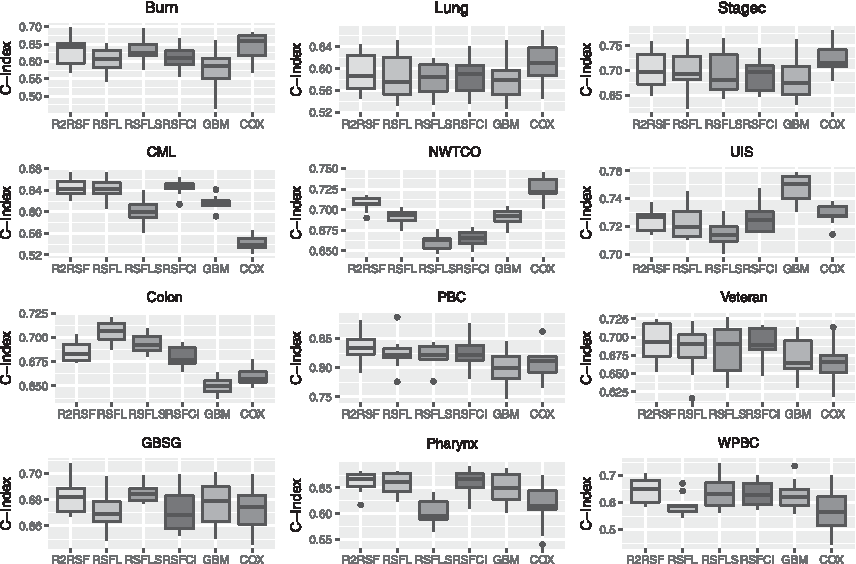
The following Figure 1 reports the performance of R2RSF, RSFL, RSFLS, RSFCI, GBM, and Cox in terms of C-index on all data sets.
Boxplots of performance in terms of C-index.
From Figure 1, one may observe that the proposed R2RSF method generally outperforms other methods on GBSG, Veteran, CML, PBC, Pharynx, and WPBC data sets. And on these data sets, Cox usually gets the worst results. This might be the situation where the proportional hazard assumption underlying Cox is violated or the parametric or semiparametric function form is not correctly specified.
From Figure 1, one may also observe that Cox generally performs better than survival forest models on Burn, Lung, NWTCO, and Stagec data sets. This might be the case wherein the proportional hazard assumption is almost satisfied. In this case, R2RSF is slightly worse than Cox but usually outperforms other survival forest models.
The Friedman rank sum test statistic on these data sets is 63.096 and it is significant as the corresponding p-value is less than 2.781e-12. Thus, to find out which pairs of models are significantly different, we can compute the Nemenyi test statistics for different pairs of survival methods. Here, we are only concerned with relative performance of the proposed model (A), and thus only Nemenyi test statistics related to model A are calculated.
The corresponding post hoc Nemenyi test results are shown in the following Table 2.
It can be seen from Table 2 that all these p-values are far <0.05. Thus, in terms of C-index, there exist significant differences between R2RSF and the other three algorithms on these data sets. In other words, based on the results on all these 12 data sets, R2RSF is significantly better than RSFL, RSFLS, RSFCI, GBM, and Cox in terms of C-index metric.
4. Conclusions
In modeling censored data, survival forest methods are a competitive nonparametric alternative to traditional parametric or semiparametric models when the functional forms are possibly misspecified or the underlying assumptions are violated.
In this work, we have proposed a survival forest approach with trees constructed using the R2 splitting rules. By studying the well-known benchmark data sets, we have found that R2RSF generally outperforms popular survival models such as RSF with log-rank, log-rank score, and C-index splitting rules, Cox proportional hazard model, and GBM in terms of C-index metric. We have also found that the proposed R2 splitting rule tends to outperform log-rank, log-rank score, or C-index splitting criteria when the proportional hazard assumption possibly holds.
It is clear that other kinds of nonparametric, semiparametric, and parametric splitting functions are available, but the goal here is to illustrate some key features of the proposed method and not to provide an exhaustive comparison across all splitting methods.
The R package and the supplementary material are available at (https://github.com/whcsu/r2rsf). The proposed algorithm still has room for improvement. First, in calculating the R2 statistic, the censoring weight is simply determined by the Kaplan–Meier estimator. Other inverse probability censoring weight schemes, such as a doubly robust extension proposed by Steingrimsson et al. (2016), might be more appropriate in certain conditions. Second, to obtain \documentclass{aastex}\usepackage{amsbsy}\usepackage{amsfonts}\usepackage{amssymb}\usepackage{bm}\usepackage{mathrsfs}\usepackage{pifont}\usepackage{stmaryrd}\usepackage{textcomp}\usepackage{portland, xspace}\usepackage{amsmath, amsxtra}\usepackage{upgreek}\pagestyle{empty}\DeclareMathSizes{10}{9}{7}{6}\begin{document}
$$m_{ \hat \theta }^{ ( wc ) } ( X_{ij}^* ( s ) )$$
\end{document} in Equation (2), we just set \documentclass{aastex}\usepackage{amsbsy}\usepackage{amsfonts}\usepackage{amssymb}\usepackage{bm}\usepackage{mathrsfs}\usepackage{pifont}\usepackage{stmaryrd}\usepackage{textcomp}\usepackage{portland, xspace}\usepackage{amsmath, amsxtra}\usepackage{upgreek}\pagestyle{empty}\DeclareMathSizes{10}{9}{7}{6}\begin{document}
$${m_{ \hat \theta }} ( X_{ij}^* ( s ) ) = X_{ij}^* ( s )$$
\end{document} for simplicity. We can further test other linear or nonlinear models to estimate \documentclass{aastex}\usepackage{amsbsy}\usepackage{amsfonts}\usepackage{amssymb}\usepackage{bm}\usepackage{mathrsfs}\usepackage{pifont}\usepackage{stmaryrd}\usepackage{textcomp}\usepackage{portland, xspace}\usepackage{amsmath, amsxtra}\usepackage{upgreek}\pagestyle{empty}\DeclareMathSizes{10}{9}{7}{6}\begin{document}
$${m_{ \hat \theta }} ( X_{ij}^* ( s ) )$$
\end{document} as well.
Footnotes
Acknowledgments
The research of Hong Wang was supported, in part, by National Social Science Foundation of China (17BTJ019). The research of X.C. was supported by the National Natural Science Foundation of China (11501573 and 11326184). The research of G.L. was partly supported by National Institute of Health Grants P30 CA-16042, UL1TR000124-02, and P01AT003960. The funders had no role in the preparation of this article. This work used computational and storage services associated with the Hoffman2 Shared Cluster provided by UCLA Institute for Digital Research and Education's Research Technology Group.
Author Disclosure Statement
No competing financial interests exist.
References
1.
BathkeA., KimM.-O., and ZhouM.2009. Combined multiple testing by censored empirical likelihood. J. Stat. Plan. Inference, 139, 814–827.
2.
Bou-HamadI., LarocqueD., and Ben-AmeurH.2011. A review of survival trees. Stat. Surv., 5, 44–71.
3.
BreimanL.2001. Random forests. Machine Learn. 45, 5–32.
4.
BreimanL., FriedmanJ., StoneC.J., et al.1984. Classification and Regression Trees. CRC Press, New York, NY.
5.
CaiT., HuangJ., and TianL.2009. Regularized estimation for the accelerated failure time model. Biometrics, 65, 394–404.
6.
CappelliC., and ZhangH.2007. Survival trees, 167–179. In Statistical Methods for Biostatistics and Related Fields. HardleW., MoriY., and VieuP. (eds.). Springer, Berlin.
7.
ChoH.J., and HongS.-M.2008. Median regression tree for analysis of censored survival data. IEEE Trans. Syst. Man Cybern. A Syst. Hum., 38, 715–726.
8.
CiampiA., ChangC.-H., HoggS., et al.1987. Recursive partition: A versatile method for exploratory-data analysis in biostatistics, pp. 23–50. In Biostatistics. MacNeillI.B., and UmphreyG. (eds.). Springer, Dordrecht.
9.
CiampiA., ThiffaultJ., NakacheJ.-P., et al.1986. Stratification by stepwise regression, correspondence analysis and recursive partition: A comparison of three methods of analysis for survival data with covariates. Comput. Stat. Data Anal., 4, 185–204.
10.
CiampiA., ThiffaultJ., and SagmanU.1989. RECPAM: A computer program for recursive partition amalgamation for censored survival data and other situations frequently occurring in biostatistics. II. applications to data on small cell carcinoma of the lung (sccl). Comput. Methods Programs Biomed., 30, 283–296.
11.
DavidC.R.1972. Regression models and life tables (with discussion). J. R. Stat. Soc., 34, 187–220.
12.
DemšarJ.2006. Statistical comparisons of classifiers over multiple data sets. J. Machine Learn. Res., 7, 1–30.
GordonL., and OlshenR.A.1985. Tree-structured survival analysis. Cancer Treat. Rep., 69, 1065–1069.
15.
HarrellF.E., LeeK.L., and MarkD.B.1996. Tutorial in biostatistics multivariable prognostic models: Issues in developing models, evaluating assumptions and adequacy, and measuring and reducing errors. Stat. Med., 15, 361–387.
16.
HothornT., BhlmannP., DudoitS., et al.2006. Survival ensembles. Biostatistics, 7, 355–373.
IshwaranH., KogalurU.B., BlackstoneE.H., et al.2008. Random survival forests. Ann. Appl. Stat., 2, 841–860.
19.
KaplanE.L., and MeierP.1958. Nonparametric estimation from incomplete observations. J. Am. Stat. Assoc., 53, 457–481.
20.
LeBlancM., and CrowleyJ.1993. Survival trees by goodness of split. J. Am. Stat. Assoc., 88, 457–467.
21.
LiG., and WangX.2016. Prediction accuracy measures for a nonlinear model and for right-censored time-to-event data. arXiv 1611.03063.
22.
MbogningC., and BroëtP.2016. Bagging survival tree procedure for variable selection and prediction in the presence of nonsusceptible patients. BMC Bioinform. 17, 230.
23.
McGeechanK., MacaskillP., IrwigL., et al.2008. Assessing new biomarkers and predictive models for use in clinical practice: A clinician's guide. Arch. Intern. Med., 168, 2304–2310.
24.
PangH., DattaD., and ZhaoH.2010. Pathway analysis using random forests with bivariate node-split for survival outcomes. Bioinformatics. 26, 250–258.
25.
PohlertT.2014. The Pairwise Multiple Comparison of Mean Ranks Package (PMCMR). R Package. Vienna, Austria.
26.
R Core Team. 2016. R: A Language and Environment for Statistical Computing. R Foundation for Statistical Computing, Vienna, Austria.
27.
RidgewayG.2004. The gbm package. R Foundation for Statistical Computing, Vienna, Austria.
28.
SchmidM., and PotapovS.2012. A comparison of estimators to evaluate the discriminatory power of time-to-event models. Stat. Med., 31, 2588–2609.
29.
SchmidM., WrightM.N., and ZieglerA.2016. On the use of Harrells C for clinical risk prediction via random survival forests. Expert Syst. Appl., 63, 450–459.
30.
SegalM.R.1988. Regression trees for censored data, 35–47. In Biometrics.
31.
ShimokawaA., KawasakiY., and MiyaokaE.2015. Comparison of splitting methods on survival tree. Int. J. Biostat., 11, 175–188.
32.
ShimokawaA., KawasakiY., and MiyaokaE.2016. A comparative study on splitting criteria of a survival tree based on the cox proportional model. J. Biopharm. Stat., 26, 386–401.