We formalize a new problem variant in gene-block discovery, denoted Reference-Anchored Gene Blocks (RAGB), given a query sequenceQof lengthn, representing the gene array of a DNA element, a window size bounddon the length of a substring of interest inQ, and a set of target gene sequences\documentclass{aastex}\usepackage{amsbsy}\usepackage{amsfonts}\usepackage{amssymb}\usepackage{bm}\usepackage{mathrsfs}\usepackage{pifont}\usepackage{stmaryrd}\usepackage{textcomp}\usepackage{portland, xspace}\usepackage{amsmath, amsxtra}\usepackage{upgreek}\pagestyle{empty}\DeclareMathSizes{10}{9}{7}{6}\begin{document}
$${ \cal T} = \{ {T_1} \ldots {T_c} \} $$
\end{document}. Our objective is to identify gene blocks in\documentclass{aastex}\usepackage{amsbsy}\usepackage{amsfonts}\usepackage{amssymb}\usepackage{bm}\usepackage{mathrsfs}\usepackage{pifont}\usepackage{stmaryrd}\usepackage{textcomp}\usepackage{portland, xspace}\usepackage{amsmath, amsxtra}\usepackage{upgreek}\pagestyle{empty}\DeclareMathSizes{10}{9}{7}{6}\begin{document}
$${ \cal T}$$
\end{document}that are centered in a subsetqof co-localized genes fromQ, and contain genomes from\documentclass{aastex}\usepackage{amsbsy}\usepackage{amsfonts}\usepackage{amssymb}\usepackage{bm}\usepackage{mathrsfs}\usepackage{pifont}\usepackage{stmaryrd}\usepackage{textcomp}\usepackage{portland, xspace}\usepackage{amsmath, amsxtra}\usepackage{upgreek}\pagestyle{empty}\DeclareMathSizes{10}{9}{7}{6}\begin{document}
$${ \cal T}$$
\end{document}in which the corresponding orthologs of the genes fromqare also co-localized. We cast RAGB as a variant of a (colored) biclique problem in bipartite graphs, and analyze its parameterized complexity, as well as the parameterized complexity of other related problems. We give an\documentclass{aastex}\usepackage{amsbsy}\usepackage{amsfonts}\usepackage{amssymb}\usepackage{bm}\usepackage{mathrsfs}\usepackage{pifont}\usepackage{stmaryrd}\usepackage{textcomp}\usepackage{portland, xspace}\usepackage{amsmath, amsxtra}\usepackage{upgreek}\pagestyle{empty}\DeclareMathSizes{10}{9}{7}{6}\begin{document}
$$O ( nm + {2^d}nm / \lg m )$$
\end{document}time algorithm for the uncolored variant of our biclique problem, wheremis the number of areas of interest that are parsed from the target sequences, andnanddare as defined earlier. Our algorithm can be adapted to compute all maximal bicliques in the graph within the same time complexity, and to handle edge weights with a slight\documentclass{aastex}\usepackage{amsbsy}\usepackage{amsfonts}\usepackage{amssymb}\usepackage{bm}\usepackage{mathrsfs}\usepackage{pifont}\usepackage{stmaryrd}\usepackage{textcomp}\usepackage{portland, xspace}\usepackage{amsmath, amsxtra}\usepackage{upgreek}\pagestyle{empty}\DeclareMathSizes{10}{9}{7}{6}\begin{document}
$$O ( \lg d )$$
\end{document}increase to its time complexity. For the colored version of the problem, our algorithm has a time complexity of\documentclass{aastex}\usepackage{amsbsy}\usepackage{amsfonts}\usepackage{amssymb}\usepackage{bm}\usepackage{mathrsfs}\usepackage{pifont}\usepackage{stmaryrd}\usepackage{textcomp}\usepackage{portland, xspace}\usepackage{amsmath, amsxtra}\usepackage{upgreek}\pagestyle{empty}\DeclareMathSizes{10}{9}{7}{6}\begin{document}
$$O{ ( 2^d}nm )$$
\end{document}. We implement the algorithm and exemplify its application to the data mining of proteobacterial gene blocks that are centered in predicted proteobacterial genomic islands, leading to the identification of putatively mobilized clusters of virulence, pathogenicity, andresistance genes.
1. Introduction
Genomes of bacterial species can evolve through a variety of processes, including mutations, rearrangements, and horizontal gene transfer. Information gathered over the past few years from a rapidly increasing number of sequenced genomes has shown that besides the core genes that encode essential metabolic functions, bacterial genomes also harbor a variable number of accessory genes acquired by horizontal gene transfer, encoding adaptive traits that might be beneficial for bacteria under certain growth or environmental conditions (Schmidt and Hensel, 2004). Many of the accessory genes acquired by horizontal gene transfer form syntenic blocks recognized as genomic islands (GIs)—discrete DNA segments that are transferred between closely related strains. During island evolution, several genetic elements may be acquired independently at different time points and from different hosts. Thus, GIs often represent mosaic-like structures rather than homogeneous segments of horizontally acquired DNA.
GIs are known to carry genes, offering a selective advantage for host bacteria. They play a key role in the emergence of highly virulent and highly resistant pathogenic strains of bacteria, which are of major concern worldwide (Schmidt and Hensel, 2004). This concern motivates new studies, such as the one proposed in this article, aimed at developing new tools that will help explore the evolution and spreading patterns of pathogenicity, virulence, and resistance components harbored within GIs, across the bacterial kingdom. Further, applying gene-block discovery approaches to these studies may shed light on the function of unknown proteins that are consistently co-transferred with functional gene cascades.
1.1. The reference-anchored gene-block problem
We propose a new bioinformatic approach that is based on interrogating a given reference DNA element from a specific genome for subsets of genes that are conserved as proximity blocks across other microbial genomes. The subsequent computational problem is called the Reference-Anchored Gene Blocks (RAGB) problem. The input to this problem consists of the gene sequence of a reference DNA element, and a set of target genome sequences. The target sequences are then parsed, either via a simple sliding window approach or according to some a priori biological data, into areas of interest or segments of small proximity. The output of our problem are gene blocks that are clustered together in a small vicinity in the reference element, and that have orthologous genes clustered together in segments of sufficiently many target genomes. Note that our model allows paralogous occurrences of genes from the reference elements (i.e., a gene may appear more than once in a target genome), and moreover, we do not require that all input genomes be represented in an output block.
Our framework is based on a bipartite graph modulation. After the phase where the input element and genomes are parsed into (gene cluster encompassing) segments, a bipartite graph is constructed according to these segments. In this graph, vertices of one side represent subsets of reference genes, nodes on the other side represent segments from the target genomes, and edges connect the subsets of reference genes to segments from the target genomes that contain corresponding orthologs. Based on this, we cast the problem of enumerating RAGB as a special type of biclustering problem: Compute appropriately constrained bicliques in an input bipartite graph. The constraint is a bound that ensures the co-localization of the reference genes participating in a block. When it is necessary to distinguish between segments of different genomes, we color-code the vertices corresponding to segments in our bipartite graph, and we require colorful bicliques as solutions.
1.2. Our contribution
Since our problem translates to a computationally hard problem, we use the theory of parameterized complexity (Downey and Fellows, 1999), which provides a convenient theoretical framework for analyzing exact algorithms for hard problems. In particular, given a bipartite graph with n vertices corresponding to references genes, and m vertices corresponding to target segments, we show how to compute all maximal constrained bicliques in \documentclass{aastex}\usepackage{amsbsy}\usepackage{amsfonts}\usepackage{amssymb}\usepackage{bm}\usepackage{mathrsfs}\usepackage{pifont}\usepackage{stmaryrd}\usepackage{textcomp}\usepackage{portland, xspace}\usepackage{amsmath, amsxtra}\usepackage{upgreek}\pagestyle{empty}\DeclareMathSizes{10}{9}{7}{6}\begin{document}
$$O ( nm + {2^d}nm / \lg m )$$
\end{document} time, where d is the bound on the genomic distance between two genes in a cluster. We then show how to extend this algorithm to a weighted variant of the problem with an \documentclass{aastex}\usepackage{amsbsy}\usepackage{amsfonts}\usepackage{amssymb}\usepackage{bm}\usepackage{mathrsfs}\usepackage{pifont}\usepackage{stmaryrd}\usepackage{textcomp}\usepackage{portland, xspace}\usepackage{amsmath, amsxtra}\usepackage{upgreek}\pagestyle{empty}\DeclareMathSizes{10}{9}{7}{6}\begin{document}
$$O ( \lg d )$$
\end{document} increase to the time complexity. Finally, our algorithm can also be extended to the more challenging vertex-colored variant corresponding to the case where segments are overlapping sliding windows in the target genomes; however, we allow only one segment per genome in the output. The time complexity increases in this case to \documentclass{aastex}\usepackage{amsbsy}\usepackage{amsfonts}\usepackage{amssymb}\usepackage{bm}\usepackage{mathrsfs}\usepackage{pifont}\usepackage{stmaryrd}\usepackage{textcomp}\usepackage{portland, xspace}\usepackage{amsmath, amsxtra}\usepackage{upgreek}\pagestyle{empty}\DeclareMathSizes{10}{9}{7}{6}\begin{document}
$$O{ ( 2^d}nm )$$
\end{document}. We also use the theory of parameterized complexity to analyze closely related biclique problems, and we show that these are unlikely to admit efficient algorithms with respect to their natural parameterizations.
We implement our algorithm in a program called RAGB Monitor. This program enumerates conserved blocks that are centered in small components of a given input DNA element and ranks them according to a probabilistic ranking score. The program is exemplified by applying it to the data mining of 33 proteobacterial genomes for gene blocks that are centered in 558 predicted proteobacterial GIs from these genomes, leading to the identification and visualization of putatively mobilized clusters of virulence, pathogenicity, and resistance genes.
1.3. Related work
A gene block is a group of genes that are consistently clustered within the same genomic vicinity across a set of genomes, regardless of the internal order of the genes from the block in each genome. The clustered occurrences of these genes within the corresponding genomes are called instances of the block. The problem of discovering gene blocks in a set of input genomes has been thoroughly studied. In the most basic variant of this problem, denoted the Common Intervals in Permutations problem (Bergeron et al., 2002; Schmidt and Stoye, 2004), a chromosome is considered a permutation of distinct genes, such that each gene appears only once in a chromosome and a gene block is defined to be a set of genes that appear in all the input genomes without gaps. A more advanced problem variant, denoted the Approximate Clusters in Permutations problem (Béal et al., 2004), extends the basic model with the relaxation of allowing gaps (intermitting genes) within the genes of block instances. Another interesting variant of this problem is the Common Intervals in Strings problem (Amir et al., 2003, 2007): Here, the genomes are modeled as general strings rather than permutations. This enables the consideration of genomes with gene duplications (paralogs). Finally, in the most advanced problem variant, the Approximate Clusters in Strings problem, gaps are allowed, duplications and missing genes among input genomes are supported, and there is no requirement that a block instance be present in all input genomes (Kim et al., 2006; Ling et al., 2009; Jahn, 2011).
The problem introduced in our article could be viewed as a special variant of gene block discovery, where the sought gene block is characterized by a specific consensus set of genes, such that orthologs of all the genes from this consensus set are required to occur, clustered together, in a designated reference genome, as well as in a predefined quorum of the other input genomes. Within this problem definition, the model we follow in our solution to the problem is the most general one: It allows paralogous occurrences of genes in the input genomes, does not require gene order conservation across distinct instances of a given gene block within the input genomes, and does not require that all input genomes participate in a candidate solution.
Note that if a gene block is not represented by a consensus gene set that is common to all instances, but rather by a closely related set with a reference occurrence in a reference genome (i.e., one without intermitting or missing genes), then the search space becomes polynomially bounded (Amir et al., 2007; Jahn, 2011). In our application, however, the sought output per gene block entails a very specific consensus descriptor, consisting of a set of genes characterizing the identified block. It is required that an ortholog of each of the genes from this consensus gene set be found in each and every instance of the block (in the designated reference genome as well as in the target genomes), allowing for intermitting genes (gaps) but not substitutions or deletions of genes from the consensus gene set. The motivation for requiring such gene-content specificity is illustrated in Section 5 where we exemplify the genomic studies toward which we aim. These studies are based on comparative analysis within “families” of gene blocks whose members differ by slight gene content variations. Such analysis requires that each gene block be characterized by its consensus genes. Of course, this requirement comes at an expense to output size: As opposed to the reference-based approaches mentioned earlier, the output of our algorithms might be exponential in the size of the input, as it entails the distinct enumeration of gene subsets from (bounded-length windows of) the designated reference genome.
2. Problem Definition and Formulations
Let \documentclass{aastex}\usepackage{amsbsy}\usepackage{amsfonts}\usepackage{amssymb}\usepackage{bm}\usepackage{mathrsfs}\usepackage{pifont}\usepackage{stmaryrd}\usepackage{textcomp}\usepackage{portland, xspace}\usepackage{amsmath, amsxtra}\usepackage{upgreek}\pagestyle{empty}\DeclareMathSizes{10}{9}{7}{6}\begin{document}
$$\Sigma$$
\end{document} denote a finite set of characters representing genes. A genome is represented by a sequence\documentclass{aastex}\usepackage{amsbsy}\usepackage{amsfonts}\usepackage{amssymb}\usepackage{bm}\usepackage{mathrsfs}\usepackage{pifont}\usepackage{stmaryrd}\usepackage{textcomp}\usepackage{portland, xspace}\usepackage{amsmath, amsxtra}\usepackage{upgreek}\pagestyle{empty}\DeclareMathSizes{10}{9}{7}{6}\begin{document}
$$S = { \sigma _1} \cdots { \sigma _n}$$
\end{document} of concatenated characters \documentclass{aastex}\usepackage{amsbsy}\usepackage{amsfonts}\usepackage{amssymb}\usepackage{bm}\usepackage{mathrsfs}\usepackage{pifont}\usepackage{stmaryrd}\usepackage{textcomp}\usepackage{portland, xspace}\usepackage{amsmath, amsxtra}\usepackage{upgreek}\pagestyle{empty}\DeclareMathSizes{10}{9}{7}{6}\begin{document}
$${ \sigma _1} , \ldots , { \sigma _n} \in \Sigma$$
\end{document}. For a sequence \documentclass{aastex}\usepackage{amsbsy}\usepackage{amsfonts}\usepackage{amssymb}\usepackage{bm}\usepackage{mathrsfs}\usepackage{pifont}\usepackage{stmaryrd}\usepackage{textcomp}\usepackage{portland, xspace}\usepackage{amsmath, amsxtra}\usepackage{upgreek}\pagestyle{empty}\DeclareMathSizes{10}{9}{7}{6}\begin{document}
$$S = { \sigma _1} \cdots { \sigma _n} ,$$
\end{document} we use \documentclass{aastex}\usepackage{amsbsy}\usepackage{amsfonts}\usepackage{amssymb}\usepackage{bm}\usepackage{mathrsfs}\usepackage{pifont}\usepackage{stmaryrd}\usepackage{textcomp}\usepackage{portland, xspace}\usepackage{amsmath, amsxtra}\usepackage{upgreek}\pagestyle{empty}\DeclareMathSizes{10}{9}{7}{6}\begin{document}
$$\vert S \vert = n$$
\end{document} to denote the length of S, and \documentclass{aastex}\usepackage{amsbsy}\usepackage{amsfonts}\usepackage{amssymb}\usepackage{bm}\usepackage{mathrsfs}\usepackage{pifont}\usepackage{stmaryrd}\usepackage{textcomp}\usepackage{portland, xspace}\usepackage{amsmath, amsxtra}\usepackage{upgreek}\pagestyle{empty}\DeclareMathSizes{10}{9}{7}{6}\begin{document}
$$S [ i ] = { \sigma _i}$$
\end{document} to denote the i'th character of S. A subsequence of S is any nonempty sequence \documentclass{aastex}\usepackage{amsbsy}\usepackage{amsfonts}\usepackage{amssymb}\usepackage{bm}\usepackage{mathrsfs}\usepackage{pifont}\usepackage{stmaryrd}\usepackage{textcomp}\usepackage{portland, xspace}\usepackage{amsmath, amsxtra}\usepackage{upgreek}\pagestyle{empty}\DeclareMathSizes{10}{9}{7}{6}\begin{document}
$$S ^{\prime}$$
\end{document} that can be obtained by deleting zero or more characters from S. An interval of S is a subsequence of S with consecutive characters. For \documentclass{aastex}\usepackage{amsbsy}\usepackage{amsfonts}\usepackage{amssymb}\usepackage{bm}\usepackage{mathrsfs}\usepackage{pifont}\usepackage{stmaryrd}\usepackage{textcomp}\usepackage{portland, xspace}\usepackage{amsmath, amsxtra}\usepackage{upgreek}\pagestyle{empty}\DeclareMathSizes{10}{9}{7}{6}\begin{document}
$$1 \le i \le j \le \vert S \vert$$
\end{document}, we let \documentclass{aastex}\usepackage{amsbsy}\usepackage{amsfonts}\usepackage{amssymb}\usepackage{bm}\usepackage{mathrsfs}\usepackage{pifont}\usepackage{stmaryrd}\usepackage{textcomp}\usepackage{portland, xspace}\usepackage{amsmath, amsxtra}\usepackage{upgreek}\pagestyle{empty}\DeclareMathSizes{10}{9}{7}{6}\begin{document}
$$S [ i , j ] = { \sigma _i} \cdots { \sigma _j}$$
\end{document} denote the interval of S beginning at position i and ending at position j. We call a sequence where all characters are different a permutation. Two sequences S1 and S2 are said to be equivalent, denoted \documentclass{aastex}\usepackage{amsbsy}\usepackage{amsfonts}\usepackage{amssymb}\usepackage{bm}\usepackage{mathrsfs}\usepackage{pifont}\usepackage{stmaryrd}\usepackage{textcomp}\usepackage{portland, xspace}\usepackage{amsmath, amsxtra}\usepackage{upgreek}\pagestyle{empty}\DeclareMathSizes{10}{9}{7}{6}\begin{document}
$${S_1} \equiv {S_2}$$
\end{document}, if \documentclass{aastex}\usepackage{amsbsy}\usepackage{amsfonts}\usepackage{amssymb}\usepackage{bm}\usepackage{mathrsfs}\usepackage{pifont}\usepackage{stmaryrd}\usepackage{textcomp}\usepackage{portland, xspace}\usepackage{amsmath, amsxtra}\usepackage{upgreek}\pagestyle{empty}\DeclareMathSizes{10}{9}{7}{6}\begin{document}
$$\vert \{ {S_1} [ i ] = \sigma :1 \le i \le \vert {S_1} \vert \} \vert = \vert \{ {S_2} [ j ] = \sigma :1 \le j \le \vert {S_2} \vert \} \vert$$
\end{document} for all \documentclass{aastex}\usepackage{amsbsy}\usepackage{amsfonts}\usepackage{amssymb}\usepackage{bm}\usepackage{mathrsfs}\usepackage{pifont}\usepackage{stmaryrd}\usepackage{textcomp}\usepackage{portland, xspace}\usepackage{amsmath, amsxtra}\usepackage{upgreek}\pagestyle{empty}\DeclareMathSizes{10}{9}{7}{6}\begin{document}
$$\sigma \in \Sigma$$
\end{document}. In other words, \documentclass{aastex}\usepackage{amsbsy}\usepackage{amsfonts}\usepackage{amssymb}\usepackage{bm}\usepackage{mathrsfs}\usepackage{pifont}\usepackage{stmaryrd}\usepackage{textcomp}\usepackage{portland, xspace}\usepackage{amsmath, amsxtra}\usepackage{upgreek}\pagestyle{empty}\DeclareMathSizes{10}{9}{7}{6}\begin{document}
$${S_1} \equiv {S_2}$$
\end{document} if both sequences have the same number of occurrences of each character \documentclass{aastex}\usepackage{amsbsy}\usepackage{amsfonts}\usepackage{amssymb}\usepackage{bm}\usepackage{mathrsfs}\usepackage{pifont}\usepackage{stmaryrd}\usepackage{textcomp}\usepackage{portland, xspace}\usepackage{amsmath, amsxtra}\usepackage{upgreek}\pagestyle{empty}\DeclareMathSizes{10}{9}{7}{6}\begin{document}
$$\sigma \in \Sigma$$
\end{document}. Clearly, for two equivalent sequences S1 and S2, we have \documentclass{aastex}\usepackage{amsbsy}\usepackage{amsfonts}\usepackage{amssymb}\usepackage{bm}\usepackage{mathrsfs}\usepackage{pifont}\usepackage{stmaryrd}\usepackage{textcomp}\usepackage{portland, xspace}\usepackage{amsmath, amsxtra}\usepackage{upgreek}\pagestyle{empty}\DeclareMathSizes{10}{9}{7}{6}\begin{document}
$$\vert {S_1} \vert = \vert {S_2} \vert$$
\end{document}.
Let Q denote a sequence representing our designated reference genome, and let \documentclass{aastex}\usepackage{amsbsy}\usepackage{amsfonts}\usepackage{amssymb}\usepackage{bm}\usepackage{mathrsfs}\usepackage{pifont}\usepackage{stmaryrd}\usepackage{textcomp}\usepackage{portland, xspace}\usepackage{amsmath, amsxtra}\usepackage{upgreek}\pagestyle{empty}\DeclareMathSizes{10}{9}{7}{6}\begin{document}
$${ \cal T} = \{ {T_1} , \ldots , {T_C} \} $$
\end{document} denote a set of sequences representing the target genomes. An instance of our problem is defined by a triplet \documentclass{aastex}\usepackage{amsbsy}\usepackage{amsfonts}\usepackage{amssymb}\usepackage{bm}\usepackage{mathrsfs}\usepackage{pifont}\usepackage{stmaryrd}\usepackage{textcomp}\usepackage{portland, xspace}\usepackage{amsmath, amsxtra}\usepackage{upgreek}\pagestyle{empty}\DeclareMathSizes{10}{9}{7}{6}\begin{document}
$$( Q , \mathcal{I} , d )$$
\end{document}, where d is a positive integer, and \documentclass{aastex}\usepackage{amsbsy}\usepackage{amsfonts}\usepackage{amssymb}\usepackage{bm}\usepackage{mathrsfs}\usepackage{pifont}\usepackage{stmaryrd}\usepackage{textcomp}\usepackage{portland, xspace}\usepackage{amsmath, amsxtra}\usepackage{upgreek}\pagestyle{empty}\DeclareMathSizes{10}{9}{7}{6}\begin{document}
$$\mathcal{I} = \{ { \mathcal{I}_1} , \ldots , { \mathcal{I}_C} \} $$
\end{document} is a family of interval sets where each \documentclass{aastex}\usepackage{amsbsy}\usepackage{amsfonts}\usepackage{amssymb}\usepackage{bm}\usepackage{mathrsfs}\usepackage{pifont}\usepackage{stmaryrd}\usepackage{textcomp}\usepackage{portland, xspace}\usepackage{amsmath, amsxtra}\usepackage{upgreek}\pagestyle{empty}\DeclareMathSizes{10}{9}{7}{6}\begin{document}
$${ \mathcal{I}_i} = \{ T_i^1 , \ldots , T_i^{{t_i}} \} $$
\end{document} contains intervals of Ti. Each interval \documentclass{aastex}\usepackage{amsbsy}\usepackage{amsfonts}\usepackage{amssymb}\usepackage{bm}\usepackage{mathrsfs}\usepackage{pifont}\usepackage{stmaryrd}\usepackage{textcomp}\usepackage{portland, xspace}\usepackage{amsmath, amsxtra}\usepackage{upgreek}\pagestyle{empty}\DeclareMathSizes{10}{9}{7}{6}\begin{document}
$$T_i^j$$
\end{document} represents an area of interest in the target genome Ti, and d represents the length of intervals that are of interest in Q. Our goal is to find subsequences in intervals of length d in Q, representing operons in the genome modeled by Q, that have equivalent occurrences in areas of interest of the target genomes. We formalized this in the following definition:
Definition 1(Block).A block in\documentclass{aastex}\usepackage{amsbsy}\usepackage{amsfonts}\usepackage{amssymb}\usepackage{bm}\usepackage{mathrsfs}\usepackage{pifont}\usepackage{stmaryrd}\usepackage{textcomp}\usepackage{portland, xspace}\usepackage{amsmath, amsxtra}\usepackage{upgreek}\pagestyle{empty}\DeclareMathSizes{10}{9}{7}{6}\begin{document}
$$( Q , \mathcal{I} , d )$$
\end{document}is a set of sequences\documentclass{aastex}\usepackage{amsbsy}\usepackage{amsfonts}\usepackage{amssymb}\usepackage{bm}\usepackage{mathrsfs}\usepackage{pifont}\usepackage{stmaryrd}\usepackage{textcomp}\usepackage{portland, xspace}\usepackage{amsmath, amsxtra}\usepackage{upgreek}\pagestyle{empty}\DeclareMathSizes{10}{9}{7}{6}\begin{document}
$$\{ q , {t_{{i_1}}} , \ldots , {t_{{i_k}}} \} $$
\end{document}satisfying:
1.q is a subsequence of some interval of length d in Q,
2.\documentclass{aastex}\usepackage{amsbsy}\usepackage{amsfonts}\usepackage{amssymb}\usepackage{bm}\usepackage{mathrsfs}\usepackage{pifont}\usepackage{stmaryrd}\usepackage{textcomp}\usepackage{portland, xspace}\usepackage{amsmath, amsxtra}\usepackage{upgreek}\pagestyle{empty}\DeclareMathSizes{10}{9}{7}{6}\begin{document}
$${t_{{i_j}}}$$
\end{document}is a subsequence of some interval in\documentclass{aastex}\usepackage{amsbsy}\usepackage{amsfonts}\usepackage{amssymb}\usepackage{bm}\usepackage{mathrsfs}\usepackage{pifont}\usepackage{stmaryrd}\usepackage{textcomp}\usepackage{portland, xspace}\usepackage{amsmath, amsxtra}\usepackage{upgreek}\pagestyle{empty}\DeclareMathSizes{10}{9}{7}{6}\begin{document}
$${ \mathcal{I}_{{i_j}}}$$
\end{document}for each\documentclass{aastex}\usepackage{amsbsy}\usepackage{amsfonts}\usepackage{amssymb}\usepackage{bm}\usepackage{mathrsfs}\usepackage{pifont}\usepackage{stmaryrd}\usepackage{textcomp}\usepackage{portland, xspace}\usepackage{amsmath, amsxtra}\usepackage{upgreek}\pagestyle{empty}\DeclareMathSizes{10}{9}{7}{6}\begin{document}
$$1 \le j \le k$$
\end{document},
We say that a block \documentclass{aastex}\usepackage{amsbsy}\usepackage{amsfonts}\usepackage{amssymb}\usepackage{bm}\usepackage{mathrsfs}\usepackage{pifont}\usepackage{stmaryrd}\usepackage{textcomp}\usepackage{portland, xspace}\usepackage{amsmath, amsxtra}\usepackage{upgreek}\pagestyle{empty}\DeclareMathSizes{10}{9}{7}{6}\begin{document}
$$\{ q , {t_{{i_1}}} , \ldots , {t_{{i_k}}} \} $$
\end{document} is maximal in \documentclass{aastex}\usepackage{amsbsy}\usepackage{amsfonts}\usepackage{amssymb}\usepackage{bm}\usepackage{mathrsfs}\usepackage{pifont}\usepackage{stmaryrd}\usepackage{textcomp}\usepackage{portland, xspace}\usepackage{amsmath, amsxtra}\usepackage{upgreek}\pagestyle{empty}\DeclareMathSizes{10}{9}{7}{6}\begin{document}
$$( Q , \mathcal{I} , d )$$
\end{document} if there is no other block \documentclass{aastex}\usepackage{amsbsy}\usepackage{amsfonts}\usepackage{amssymb}\usepackage{bm}\usepackage{mathrsfs}\usepackage{pifont}\usepackage{stmaryrd}\usepackage{textcomp}\usepackage{portland, xspace}\usepackage{amsmath, amsxtra}\usepackage{upgreek}\pagestyle{empty}\DeclareMathSizes{10}{9}{7}{6}\begin{document}
$$\{ q ^{\prime} , {t ^{\prime} _{{j_1}}} , \ldots , {t ^{\prime} _{{j_ \ell }}} \} $$
\end{document} in this instance where q is a subsequence of \documentclass{aastex}\usepackage{amsbsy}\usepackage{amsfonts}\usepackage{amssymb}\usepackage{bm}\usepackage{mathrsfs}\usepackage{pifont}\usepackage{stmaryrd}\usepackage{textcomp}\usepackage{portland, xspace}\usepackage{amsmath, amsxtra}\usepackage{upgreek}\pagestyle{empty}\DeclareMathSizes{10}{9}{7}{6}\begin{document}
$$q ^{\prime}$$
\end{document} and \documentclass{aastex}\usepackage{amsbsy}\usepackage{amsfonts}\usepackage{amssymb}\usepackage{bm}\usepackage{mathrsfs}\usepackage{pifont}\usepackage{stmaryrd}\usepackage{textcomp}\usepackage{portland, xspace}\usepackage{amsmath, amsxtra}\usepackage{upgreek}\pagestyle{empty}\DeclareMathSizes{10}{9}{7}{6}\begin{document}
$$\{ {i_1} , \ldots , {i_k} \} \subseteq \{ {j_1} , \ldots , {j_ \ell } \} $$
\end{document}.
Definition 2 (RAGB Problem). The RAGB problem is the problem of computing all maximal blocks in a given problem instance\documentclass{aastex}\usepackage{amsbsy}\usepackage{amsfonts}\usepackage{amssymb}\usepackage{bm}\usepackage{mathrsfs}\usepackage{pifont}\usepackage{stmaryrd}\usepackage{textcomp}\usepackage{portland, xspace}\usepackage{amsmath, amsxtra}\usepackage{upgreek}\pagestyle{empty}\DeclareMathSizes{10}{9}{7}{6}\begin{document}
$$( Q , \mathcal{I} , d )$$
\end{document}.
We consider two distinct approaches to parse the intervals of our target genomes. The first approach, which we call the sliding window approach, is an exhaustive approach where each target genome in Ti is parsed into all its substrings of length d, that is, \documentclass{aastex}\usepackage{amsbsy}\usepackage{amsfonts}\usepackage{amssymb}\usepackage{bm}\usepackage{mathrsfs}\usepackage{pifont}\usepackage{stmaryrd}\usepackage{textcomp}\usepackage{portland, xspace}\usepackage{amsmath, amsxtra}\usepackage{upgreek}\pagestyle{empty}\DeclareMathSizes{10}{9}{7}{6}\begin{document}
$${T_i} [ 1 , d ] , {T_i} [ 2 , d + 1 ] , \ldots , {T_i} [ n - d , n ]$$
\end{document}, and each such substring yields an interval in \documentclass{aastex}\usepackage{amsbsy}\usepackage{amsfonts}\usepackage{amssymb}\usepackage{bm}\usepackage{mathrsfs}\usepackage{pifont}\usepackage{stmaryrd}\usepackage{textcomp}\usepackage{portland, xspace}\usepackage{amsmath, amsxtra}\usepackage{upgreek}\pagestyle{empty}\DeclareMathSizes{10}{9}{7}{6}\begin{document}
$${ \mathcal{I}_i}$$
\end{document}. The second approach takes into account biological signals to parse the genome into nonoverlapping intervals. Another modeling option to be considered is whether we allow one or more orthologous genes in each of our input genomes, that is, whether or not our input sequences are permutations. This leads to the following two RAGB problem variants:
RAGB1: Compute reference-anchored gene clusters in the following model: Intervals in \documentclass{aastex}\usepackage{amsbsy}\usepackage{amsfonts}\usepackage{amssymb}\usepackage{bm}\usepackage{mathrsfs}\usepackage{pifont}\usepackage{stmaryrd}\usepackage{textcomp}\usepackage{portland, xspace}\usepackage{amsmath, amsxtra}\usepackage{upgreek}\pagestyle{empty}\DeclareMathSizes{10}{9}{7}{6}\begin{document}
$$\mathcal{I}$$
\end{document} are parsed biologically into nonoverlapping intervals. All input sequences are permutations.
RAGB2: Compute reference-anchored gene clusters in the following model: Intervals in \documentclass{aastex}\usepackage{amsbsy}\usepackage{amsfonts}\usepackage{amssymb}\usepackage{bm}\usepackage{mathrsfs}\usepackage{pifont}\usepackage{stmaryrd}\usepackage{textcomp}\usepackage{portland, xspace}\usepackage{amsmath, amsxtra}\usepackage{upgreek}\pagestyle{empty}\DeclareMathSizes{10}{9}{7}{6}\begin{document}
$$\mathcal{I}$$
\end{document} are parsed via the sliding window approach. The input sequences are not necessarily permutations.
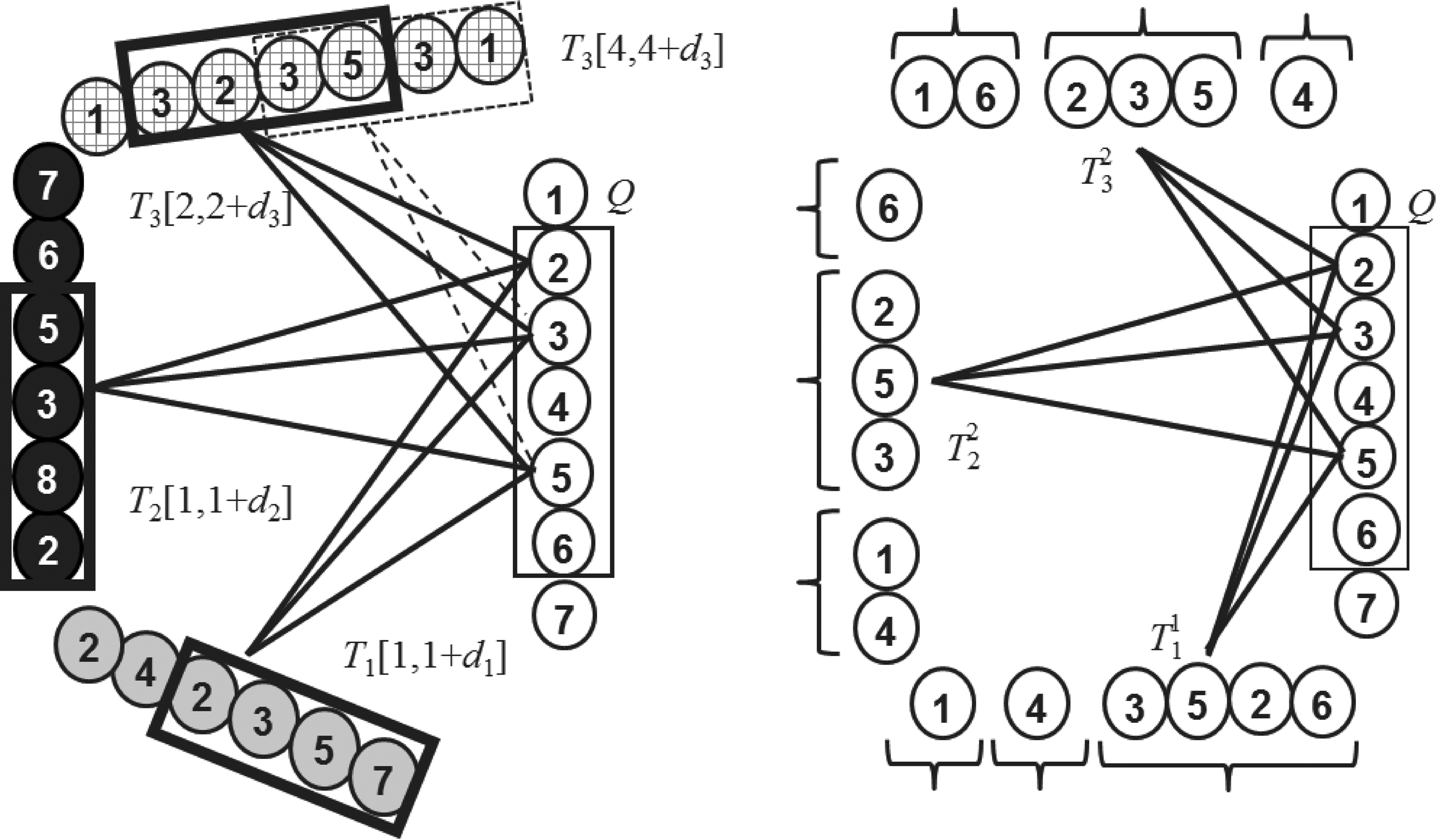
Figure 1 illustrates our general framework for solving both variants of RAGB. We cast each variant as a biclique enumeration problem in a bipartite graph. The input to our framework consists of a sequence Q representing our designated genome, and \documentclass{aastex}\usepackage{amsbsy}\usepackage{amsfonts}\usepackage{amssymb}\usepackage{bm}\usepackage{mathrsfs}\usepackage{pifont}\usepackage{stmaryrd}\usepackage{textcomp}\usepackage{portland, xspace}\usepackage{amsmath, amsxtra}\usepackage{upgreek}\pagestyle{empty}\DeclareMathSizes{10}{9}{7}{6}\begin{document}
$${T_1} , \ldots , {T_C}$$
\end{document} sequences representing the reference genomes. Each genome Ti is parsed into intervals, and the ensemble of intervals from all the genomes yields the interval set \documentclass{aastex}\usepackage{amsbsy}\usepackage{amsfonts}\usepackage{amssymb}\usepackage{bm}\usepackage{mathrsfs}\usepackage{pifont}\usepackage{stmaryrd}\usepackage{textcomp}\usepackage{portland, xspace}\usepackage{amsmath, amsxtra}\usepackage{upgreek}\pagestyle{empty}\DeclareMathSizes{10}{9}{7}{6}\begin{document}
$$\mathcal{I} = \{ { \mathcal{I}_1} , \ldots , { \mathcal{I}_C} \} $$
\end{document}.
A depiction of the two problem variants of RAGB: On the right, all sequences are permutations, and the target genomes were parsed according to biological information that resulted in nonoverlapping intervals (RAGB1). On the left, the sequences are not assumed to be permutations, and the sliding window approach was used for parsing, resulting in overlapping windows (RAGB2). On both sides, a four-block biclique with nine edges is depicted. RAGB, Reference-Anchored Gene Blocks. Box in reference genome Q illustrates an interval from which subsets of genes are enumerated for candidate block discovery. Boxes in genomes T1, T2, and T3 illustrate sliding windows that are instances of the gene-set {2,3,5}. Dotted box in genome T3 illustrates a sliding window that could serve as an instance of the gene-set {3,5}, jointly with the boxed windows in genomes T1 and T2.
Based on Q and the intervals in \documentclass{aastex}\usepackage{amsbsy}\usepackage{amsfonts}\usepackage{amssymb}\usepackage{bm}\usepackage{mathrsfs}\usepackage{pifont}\usepackage{stmaryrd}\usepackage{textcomp}\usepackage{portland, xspace}\usepackage{amsmath, amsxtra}\usepackage{upgreek}\pagestyle{empty}\DeclareMathSizes{10}{9}{7}{6}\begin{document}
$$\mathcal{I}$$
\end{document}, a bipartite graph \documentclass{aastex}\usepackage{amsbsy}\usepackage{amsfonts}\usepackage{amssymb}\usepackage{bm}\usepackage{mathrsfs}\usepackage{pifont}\usepackage{stmaryrd}\usepackage{textcomp}\usepackage{portland, xspace}\usepackage{amsmath, amsxtra}\usepackage{upgreek}\pagestyle{empty}\DeclareMathSizes{10}{9}{7}{6}\begin{document}
$$G = ( A \uplus B , E )$$
\end{document} is constructed: Each node in \documentclass{aastex}\usepackage{amsbsy}\usepackage{amsfonts}\usepackage{amssymb}\usepackage{bm}\usepackage{mathrsfs}\usepackage{pifont}\usepackage{stmaryrd}\usepackage{textcomp}\usepackage{portland, xspace}\usepackage{amsmath, amsxtra}\usepackage{upgreek}\pagestyle{empty}\DeclareMathSizes{10}{9}{7}{6}\begin{document}
$$A =\{ {a_1} , \ldots , {a_n} \} $$
\end{document} represents a single character in Q, such that node \documentclass{aastex}\usepackage{amsbsy}\usepackage{amsfonts}\usepackage{amssymb}\usepackage{bm}\usepackage{mathrsfs}\usepackage{pifont}\usepackage{stmaryrd}\usepackage{textcomp}\usepackage{portland, xspace}\usepackage{amsmath, amsxtra}\usepackage{upgreek}\pagestyle{empty}\DeclareMathSizes{10}{9}{7}{6}\begin{document}
$${a_i} \in A$$
\end{document} corresponds to the character \documentclass{aastex}\usepackage{amsbsy}\usepackage{amsfonts}\usepackage{amssymb}\usepackage{bm}\usepackage{mathrsfs}\usepackage{pifont}\usepackage{stmaryrd}\usepackage{textcomp}\usepackage{portland, xspace}\usepackage{amsmath, amsxtra}\usepackage{upgreek}\pagestyle{empty}\DeclareMathSizes{10}{9}{7}{6}\begin{document}
$$Q [ j ]$$
\end{document}. Each node in \documentclass{aastex}\usepackage{amsbsy}\usepackage{amsfonts}\usepackage{amssymb}\usepackage{bm}\usepackage{mathrsfs}\usepackage{pifont}\usepackage{stmaryrd}\usepackage{textcomp}\usepackage{portland, xspace}\usepackage{amsmath, amsxtra}\usepackage{upgreek}\pagestyle{empty}\DeclareMathSizes{10}{9}{7}{6}\begin{document}
$$B = \{ {b_1} , \ldots , {b_m} \} $$
\end{document} represents a distinct interval in \documentclass{aastex}\usepackage{amsbsy}\usepackage{amsfonts}\usepackage{amssymb}\usepackage{bm}\usepackage{mathrsfs}\usepackage{pifont}\usepackage{stmaryrd}\usepackage{textcomp}\usepackage{portland, xspace}\usepackage{amsmath, amsxtra}\usepackage{upgreek}\pagestyle{empty}\DeclareMathSizes{10}{9}{7}{6}\begin{document}
$$\mathcal{I}$$
\end{document}. We then connect vertex \documentclass{aastex}\usepackage{amsbsy}\usepackage{amsfonts}\usepackage{amssymb}\usepackage{bm}\usepackage{mathrsfs}\usepackage{pifont}\usepackage{stmaryrd}\usepackage{textcomp}\usepackage{portland, xspace}\usepackage{amsmath, amsxtra}\usepackage{upgreek}\pagestyle{empty}\DeclareMathSizes{10}{9}{7}{6}\begin{document}
$${a_i} \in A$$
\end{document} to vertex \documentclass{aastex}\usepackage{amsbsy}\usepackage{amsfonts}\usepackage{amssymb}\usepackage{bm}\usepackage{mathrsfs}\usepackage{pifont}\usepackage{stmaryrd}\usepackage{textcomp}\usepackage{portland, xspace}\usepackage{amsmath, amsxtra}\usepackage{upgreek}\pagestyle{empty}\DeclareMathSizes{10}{9}{7}{6}\begin{document}
$${b_j} \in B$$
\end{document} if the character \documentclass{aastex}\usepackage{amsbsy}\usepackage{amsfonts}\usepackage{amssymb}\usepackage{bm}\usepackage{mathrsfs}\usepackage{pifont}\usepackage{stmaryrd}\usepackage{textcomp}\usepackage{portland, xspace}\usepackage{amsmath, amsxtra}\usepackage{upgreek}\pagestyle{empty}\DeclareMathSizes{10}{9}{7}{6}\begin{document}
$$Q [ i ]$$
\end{document} appears in the interval corresponding to bj. We can also add a weight measure to this edge to indicate the level of similarity between the gene \documentclass{aastex}\usepackage{amsbsy}\usepackage{amsfonts}\usepackage{amssymb}\usepackage{bm}\usepackage{mathrsfs}\usepackage{pifont}\usepackage{stmaryrd}\usepackage{textcomp}\usepackage{portland, xspace}\usepackage{amsmath, amsxtra}\usepackage{upgreek}\pagestyle{empty}\DeclareMathSizes{10}{9}{7}{6}\begin{document}
$$Q [ i ]$$
\end{document} and its occurrence in the interval corresponding to bj. Next, for the second variant of RAGB, we need to distinguish between intervals of different genomes. For this, we introduce a coloring function\documentclass{aastex}\usepackage{amsbsy}\usepackage{amsfonts}\usepackage{amssymb}\usepackage{bm}\usepackage{mathrsfs}\usepackage{pifont}\usepackage{stmaryrd}\usepackage{textcomp}\usepackage{portland, xspace}\usepackage{amsmath, amsxtra}\usepackage{upgreek}\pagestyle{empty}\DeclareMathSizes{10}{9}{7}{6}\begin{document}
$$c:B \to \{ 1 , \ldots , C \} $$
\end{document} for the vertices of B, where \documentclass{aastex}\usepackage{amsbsy}\usepackage{amsfonts}\usepackage{amssymb}\usepackage{bm}\usepackage{mathrsfs}\usepackage{pifont}\usepackage{stmaryrd}\usepackage{textcomp}\usepackage{portland, xspace}\usepackage{amsmath, amsxtra}\usepackage{upgreek}\pagestyle{empty}\DeclareMathSizes{10}{9}{7}{6}\begin{document}
$$c ( {b_j} ) = i$$
\end{document} if bj corresponds to an interval of Ti. The reason that we do not need this function for RAGB1 is that each sequence Ti is a permutation, so any character of Q can appear at most once in any of these sequences.
A biclique in G is a pair of nonempty vertex subsets \documentclass{aastex}\usepackage{amsbsy}\usepackage{amsfonts}\usepackage{amssymb}\usepackage{bm}\usepackage{mathrsfs}\usepackage{pifont}\usepackage{stmaryrd}\usepackage{textcomp}\usepackage{portland, xspace}\usepackage{amsmath, amsxtra}\usepackage{upgreek}\pagestyle{empty}\DeclareMathSizes{10}{9}{7}{6}\begin{document}
$$A ^{\prime} \subseteq A$$
\end{document} and \documentclass{aastex}\usepackage{amsbsy}\usepackage{amsfonts}\usepackage{amssymb}\usepackage{bm}\usepackage{mathrsfs}\usepackage{pifont}\usepackage{stmaryrd}\usepackage{textcomp}\usepackage{portland, xspace}\usepackage{amsmath, amsxtra}\usepackage{upgreek}\pagestyle{empty}\DeclareMathSizes{10}{9}{7}{6}\begin{document}
$$B ^{\prime} \subseteq B$$
\end{document}, where \documentclass{aastex}\usepackage{amsbsy}\usepackage{amsfonts}\usepackage{amssymb}\usepackage{bm}\usepackage{mathrsfs}\usepackage{pifont}\usepackage{stmaryrd}\usepackage{textcomp}\usepackage{portland, xspace}\usepackage{amsmath, amsxtra}\usepackage{upgreek}\pagestyle{empty}\DeclareMathSizes{10}{9}{7}{6}\begin{document}
$$\{ a , b \} \in E$$
\end{document} for each pair of vertices \documentclass{aastex}\usepackage{amsbsy}\usepackage{amsfonts}\usepackage{amssymb}\usepackage{bm}\usepackage{mathrsfs}\usepackage{pifont}\usepackage{stmaryrd}\usepackage{textcomp}\usepackage{portland, xspace}\usepackage{amsmath, amsxtra}\usepackage{upgreek}\pagestyle{empty}\DeclareMathSizes{10}{9}{7}{6}\begin{document}
$$a \in A ^{\prime}$$
\end{document} and \documentclass{aastex}\usepackage{amsbsy}\usepackage{amsfonts}\usepackage{amssymb}\usepackage{bm}\usepackage{mathrsfs}\usepackage{pifont}\usepackage{stmaryrd}\usepackage{textcomp}\usepackage{portland, xspace}\usepackage{amsmath, amsxtra}\usepackage{upgreek}\pagestyle{empty}\DeclareMathSizes{10}{9}{7}{6}\begin{document}
$$b \in B ^{\prime}$$
\end{document}. We say that a biclique \documentclass{aastex}\usepackage{amsbsy}\usepackage{amsfonts}\usepackage{amssymb}\usepackage{bm}\usepackage{mathrsfs}\usepackage{pifont}\usepackage{stmaryrd}\usepackage{textcomp}\usepackage{portland, xspace}\usepackage{amsmath, amsxtra}\usepackage{upgreek}\pagestyle{empty}\DeclareMathSizes{10}{9}{7}{6}\begin{document}
$$( A ^{\prime} , B ^{\prime} )$$
\end{document} is maximal if for any biclique \documentclass{aastex}\usepackage{amsbsy}\usepackage{amsfonts}\usepackage{amssymb}\usepackage{bm}\usepackage{mathrsfs}\usepackage{pifont}\usepackage{stmaryrd}\usepackage{textcomp}\usepackage{portland, xspace}\usepackage{amsmath, amsxtra}\usepackage{upgreek}\pagestyle{empty}\DeclareMathSizes{10}{9}{7}{6}\begin{document}
$$( A ^{\prime \prime} , B ^{\prime \prime} )$$
\end{document} in G with \documentclass{aastex}\usepackage{amsbsy}\usepackage{amsfonts}\usepackage{amssymb}\usepackage{bm}\usepackage{mathrsfs}\usepackage{pifont}\usepackage{stmaryrd}\usepackage{textcomp}\usepackage{portland, xspace}\usepackage{amsmath, amsxtra}\usepackage{upgreek}\pagestyle{empty}\DeclareMathSizes{10}{9}{7}{6}\begin{document}
$$A ^{\prime} \subseteq A ^{\prime \prime}$$
\end{document} and \documentclass{aastex}\usepackage{amsbsy}\usepackage{amsfonts}\usepackage{amssymb}\usepackage{bm}\usepackage{mathrsfs}\usepackage{pifont}\usepackage{stmaryrd}\usepackage{textcomp}\usepackage{portland, xspace}\usepackage{amsmath, amsxtra}\usepackage{upgreek}\pagestyle{empty}\DeclareMathSizes{10}{9}{7}{6}\begin{document}
$$B ^{\prime} \subseteq B ^{\prime \prime}$$
\end{document} we have \documentclass{aastex}\usepackage{amsbsy}\usepackage{amsfonts}\usepackage{amssymb}\usepackage{bm}\usepackage{mathrsfs}\usepackage{pifont}\usepackage{stmaryrd}\usepackage{textcomp}\usepackage{portland, xspace}\usepackage{amsmath, amsxtra}\usepackage{upgreek}\pagestyle{empty}\DeclareMathSizes{10}{9}{7}{6}\begin{document}
$$A ^{\prime} = A ^{\prime \prime}$$
\end{document} and \documentclass{aastex}\usepackage{amsbsy}\usepackage{amsfonts}\usepackage{amssymb}\usepackage{bm}\usepackage{mathrsfs}\usepackage{pifont}\usepackage{stmaryrd}\usepackage{textcomp}\usepackage{portland, xspace}\usepackage{amsmath, amsxtra}\usepackage{upgreek}\pagestyle{empty}\DeclareMathSizes{10}{9}{7}{6}\begin{document}
$$B ^{\prime} = B ^{\prime \prime}$$
\end{document}. In case G is equipped with a coloring function for the vertices in B, we say that a biclique \documentclass{aastex}\usepackage{amsbsy}\usepackage{amsfonts}\usepackage{amssymb}\usepackage{bm}\usepackage{mathrsfs}\usepackage{pifont}\usepackage{stmaryrd}\usepackage{textcomp}\usepackage{portland, xspace}\usepackage{amsmath, amsxtra}\usepackage{upgreek}\pagestyle{empty}\DeclareMathSizes{10}{9}{7}{6}\begin{document}
$$( A ^{\prime} , B ^{\prime} )$$
\end{document} is colorful if no two distinct vertices in \documentclass{aastex}\usepackage{amsbsy}\usepackage{amsfonts}\usepackage{amssymb}\usepackage{bm}\usepackage{mathrsfs}\usepackage{pifont}\usepackage{stmaryrd}\usepackage{textcomp}\usepackage{portland, xspace}\usepackage{amsmath, amsxtra}\usepackage{upgreek}\pagestyle{empty}\DeclareMathSizes{10}{9}{7}{6}\begin{document}
$$B ^{\prime}$$
\end{document} have the same color. For \documentclass{aastex}\usepackage{amsbsy}\usepackage{amsfonts}\usepackage{amssymb}\usepackage{bm}\usepackage{mathrsfs}\usepackage{pifont}\usepackage{stmaryrd}\usepackage{textcomp}\usepackage{portland, xspace}\usepackage{amsmath, amsxtra}\usepackage{upgreek}\pagestyle{empty}\DeclareMathSizes{10}{9}{7}{6}\begin{document}
$$1 \le i \le n - d$$
\end{document}, let \documentclass{aastex}\usepackage{amsbsy}\usepackage{amsfonts}\usepackage{amssymb}\usepackage{bm}\usepackage{mathrsfs}\usepackage{pifont}\usepackage{stmaryrd}\usepackage{textcomp}\usepackage{portland, xspace}\usepackage{amsmath, amsxtra}\usepackage{upgreek}\pagestyle{empty}\DeclareMathSizes{10}{9}{7}{6}\begin{document}
$$A [ i , i + d ]$$
\end{document} denote the subset of vertices \documentclass{aastex}\usepackage{amsbsy}\usepackage{amsfonts}\usepackage{amssymb}\usepackage{bm}\usepackage{mathrsfs}\usepackage{pifont}\usepackage{stmaryrd}\usepackage{textcomp}\usepackage{portland, xspace}\usepackage{amsmath, amsxtra}\usepackage{upgreek}\pagestyle{empty}\DeclareMathSizes{10}{9}{7}{6}\begin{document}
$$\{ {a_i} , {a_{i + 1}} , \ldots , {a_{i + d}} \} \subseteq A$$
\end{document}.
Observation 1.There is one-to-one bijection between maximal (colorful) bicliques\documentclass{aastex}\usepackage{amsbsy}\usepackage{amsfonts}\usepackage{amssymb}\usepackage{bm}\usepackage{mathrsfs}\usepackage{pifont}\usepackage{stmaryrd}\usepackage{textcomp}\usepackage{portland, xspace}\usepackage{amsmath, amsxtra}\usepackage{upgreek}\pagestyle{empty}\DeclareMathSizes{10}{9}{7}{6}\begin{document}
$$( A ^{\prime} , B ^{\prime} )$$
\end{document}in G with\documentclass{aastex}\usepackage{amsbsy}\usepackage{amsfonts}\usepackage{amssymb}\usepackage{bm}\usepackage{mathrsfs}\usepackage{pifont}\usepackage{stmaryrd}\usepackage{textcomp}\usepackage{portland, xspace}\usepackage{amsmath, amsxtra}\usepackage{upgreek}\pagestyle{empty}\DeclareMathSizes{10}{9}{7}{6}\begin{document}
$$A ^{\prime} \subseteq A [ i , i + d ]$$
\end{document}for some\documentclass{aastex}\usepackage{amsbsy}\usepackage{amsfonts}\usepackage{amssymb}\usepackage{bm}\usepackage{mathrsfs}\usepackage{pifont}\usepackage{stmaryrd}\usepackage{textcomp}\usepackage{portland, xspace}\usepackage{amsmath, amsxtra}\usepackage{upgreek}\pagestyle{empty}\DeclareMathSizes{10}{9}{7}{6}\begin{document}
$$1 \le i \le n - d$$
\end{document}and maximal blocks in\documentclass{aastex}\usepackage{amsbsy}\usepackage{amsfonts}\usepackage{amssymb}\usepackage{bm}\usepackage{mathrsfs}\usepackage{pifont}\usepackage{stmaryrd}\usepackage{textcomp}\usepackage{portland, xspace}\usepackage{amsmath, amsxtra}\usepackage{upgreek}\pagestyle{empty}\DeclareMathSizes{10}{9}{7}{6}\begin{document}
$$( Q , \mathcal{I} , d )$$
\end{document}.
2.1. Parameterized complexity primer
We are interested in computing bicliques of certain properties in a bipartite graph. Since computing a biclique with a certain number of edges or vertices in a bipartite graph is NP complete (Garey and Johnson, 1979), any meaningful model for our problem will be non-deterministic polynomial time (NP) hard as well. Thus, we use the theory of parameterized complexity (Downey and Fellows, 1999) to cope with this hardness. Next, we provide a brief description of this theory, only mentioning elements that will be relevant for our scope.
Parameterized complexity facilitates the analysis of computational problems in terms of various instance parameters that may be independent of the total input length. In this way, problem instances are analyzed not only according to the total input length n but also according to an additional numerical parameter k that may encode other aspects of the input. Thus, formally a parameterized problem is a set of ordered pairs \documentclass{aastex}\usepackage{amsbsy}\usepackage{amsfonts}\usepackage{amssymb}\usepackage{bm}\usepackage{mathrsfs}\usepackage{pifont}\usepackage{stmaryrd}\usepackage{textcomp}\usepackage{portland, xspace}\usepackage{amsmath, amsxtra}\usepackage{upgreek}\pagestyle{empty}\DeclareMathSizes{10}{9}{7}{6}\begin{document}
$$( x , k ) \in { \{ 0 , 1 \} ^*} \times \mathbb{N}$$
\end{document}, where x encodes the combinatorial aspects of the input, and k is the parameter. A parameterized problem is considered tractable (formally, fixed-parameter tractable [FPT] for short) if there is an algorithm solving any instance \documentclass{aastex}\usepackage{amsbsy}\usepackage{amsfonts}\usepackage{amssymb}\usepackage{bm}\usepackage{mathrsfs}\usepackage{pifont}\usepackage{stmaryrd}\usepackage{textcomp}\usepackage{portland, xspace}\usepackage{amsmath, amsxtra}\usepackage{upgreek}\pagestyle{empty}\DeclareMathSizes{10}{9}{7}{6}\begin{document}
$$( x , k )$$
\end{document} in \documentclass{aastex}\usepackage{amsbsy}\usepackage{amsfonts}\usepackage{amssymb}\usepackage{bm}\usepackage{mathrsfs}\usepackage{pifont}\usepackage{stmaryrd}\usepackage{textcomp}\usepackage{portland, xspace}\usepackage{amsmath, amsxtra}\usepackage{upgreek}\pagestyle{empty}\DeclareMathSizes{10}{9}{7}{6}\begin{document}
$$f ( k ) \cdot \vert x{ \vert ^{O ( 1 ) }}$$
\end{document} time, where \documentclass{aastex}\usepackage{amsbsy}\usepackage{amsfonts}\usepackage{amssymb}\usepackage{bm}\usepackage{mathrsfs}\usepackage{pifont}\usepackage{stmaryrd}\usepackage{textcomp}\usepackage{portland, xspace}\usepackage{amsmath, amsxtra}\usepackage{upgreek}\pagestyle{empty}\DeclareMathSizes{10}{9}{7}{6}\begin{document}
$$f ( )$$
\end{document} is allowed to be any arbitrary (even exponential) computable function that is independent of \documentclass{aastex}\usepackage{amsbsy}\usepackage{amsfonts}\usepackage{amssymb}\usepackage{bm}\usepackage{mathrsfs}\usepackage{pifont}\usepackage{stmaryrd}\usepackage{textcomp}\usepackage{portland, xspace}\usepackage{amsmath, amsxtra}\usepackage{upgreek}\pagestyle{empty}\DeclareMathSizes{10}{9}{7}{6}\begin{document}
$$\vert x \vert$$
\end{document} (the input length), and the exponent in \documentclass{aastex}\usepackage{amsbsy}\usepackage{amsfonts}\usepackage{amssymb}\usepackage{bm}\usepackage{mathrsfs}\usepackage{pifont}\usepackage{stmaryrd}\usepackage{textcomp}\usepackage{portland, xspace}\usepackage{amsmath, amsxtra}\usepackage{upgreek}\pagestyle{empty}\DeclareMathSizes{10}{9}{7}{6}\begin{document}
$$\vert x{ \vert ^{O ( 1 ) }}$$
\end{document} is required to be independent of k. For example, a running time of \documentclass{aastex}\usepackage{amsbsy}\usepackage{amsfonts}\usepackage{amssymb}\usepackage{bm}\usepackage{mathrsfs}\usepackage{pifont}\usepackage{stmaryrd}\usepackage{textcomp}\usepackage{portland, xspace}\usepackage{amsmath, amsxtra}\usepackage{upgreek}\pagestyle{empty}\DeclareMathSizes{10}{9}{7}{6}\begin{document}
$${2^{O ( k ) }} \cdot {n^3}$$
\end{document} is considered feasible in the parameterized setting, whereas \documentclass{aastex}\usepackage{amsbsy}\usepackage{amsfonts}\usepackage{amssymb}\usepackage{bm}\usepackage{mathrsfs}\usepackage{pifont}\usepackage{stmaryrd}\usepackage{textcomp}\usepackage{portland, xspace}\usepackage{amsmath, amsxtra}\usepackage{upgreek}\pagestyle{empty}\DeclareMathSizes{10}{9}{7}{6}\begin{document}
$${n^{O ( k ) }}$$
\end{document} is considered infeasible. In this way, we can model scenarios where certain problem parameters are typically much smaller than the total input length, yet may not be small enough to be considered constant.
The most common way of showing that a certain parameterized problem is unlikely to have an \documentclass{aastex}\usepackage{amsbsy}\usepackage{amsfonts}\usepackage{amssymb}\usepackage{bm}\usepackage{mathrsfs}\usepackage{pifont}\usepackage{stmaryrd}\usepackage{textcomp}\usepackage{portland, xspace}\usepackage{amsmath, amsxtra}\usepackage{upgreek}\pagestyle{empty}\DeclareMathSizes{10}{9}{7}{6}\begin{document}
$$f ( k ) \cdot \vert x{ \vert ^{O ( 1 ) }}$$
\end{document} time algorithm is via a parameterized reduction from a problem, which is hard for W[1], a class of problems that may be considered the parameterized analog of NP. A parameterized reduction from a parameterized problem \documentclass{aastex}\usepackage{amsbsy}\usepackage{amsfonts}\usepackage{amssymb}\usepackage{bm}\usepackage{mathrsfs}\usepackage{pifont}\usepackage{stmaryrd}\usepackage{textcomp}\usepackage{portland, xspace}\usepackage{amsmath, amsxtra}\usepackage{upgreek}\pagestyle{empty}\DeclareMathSizes{10}{9}{7}{6}\begin{document}
$${L_1} \subseteq { \{ 0 , 1 \} ^*} \times \mathbb{N}$$
\end{document} to a parameterized problem \documentclass{aastex}\usepackage{amsbsy}\usepackage{amsfonts}\usepackage{amssymb}\usepackage{bm}\usepackage{mathrsfs}\usepackage{pifont}\usepackage{stmaryrd}\usepackage{textcomp}\usepackage{portland, xspace}\usepackage{amsmath, amsxtra}\usepackage{upgreek}\pagestyle{empty}\DeclareMathSizes{10}{9}{7}{6}\begin{document}
$${L_2} \subseteq { \{ 0 , 1 \} ^*} \times \mathbb{N}$$
\end{document} is an algorithm that, on input \documentclass{aastex}\usepackage{amsbsy}\usepackage{amsfonts}\usepackage{amssymb}\usepackage{bm}\usepackage{mathrsfs}\usepackage{pifont}\usepackage{stmaryrd}\usepackage{textcomp}\usepackage{portland, xspace}\usepackage{amsmath, amsxtra}\usepackage{upgreek}\pagestyle{empty}\DeclareMathSizes{10}{9}{7}{6}\begin{document}
$$( x , k ) \in { \{ 0 , 1 \} ^*} \times \mathbb{N}$$
\end{document}, outputs an instance \documentclass{aastex}\usepackage{amsbsy}\usepackage{amsfonts}\usepackage{amssymb}\usepackage{bm}\usepackage{mathrsfs}\usepackage{pifont}\usepackage{stmaryrd}\usepackage{textcomp}\usepackage{portland, xspace}\usepackage{amsmath, amsxtra}\usepackage{upgreek}\pagestyle{empty}\DeclareMathSizes{10}{9}{7}{6}\begin{document}
$$( x ^{\prime} , k ^{\prime} ) \in { \{ 0 , 1 \} ^*} \times \mathbb{N}$$
\end{document} in \documentclass{aastex}\usepackage{amsbsy}\usepackage{amsfonts}\usepackage{amssymb}\usepackage{bm}\usepackage{mathrsfs}\usepackage{pifont}\usepackage{stmaryrd}\usepackage{textcomp}\usepackage{portland, xspace}\usepackage{amsmath, amsxtra}\usepackage{upgreek}\pagestyle{empty}\DeclareMathSizes{10}{9}{7}{6}\begin{document}
$$f ( k ) \cdot poly ( \vert x \vert )$$
\end{document} time, for some fixed function \documentclass{aastex}\usepackage{amsbsy}\usepackage{amsfonts}\usepackage{amssymb}\usepackage{bm}\usepackage{mathrsfs}\usepackage{pifont}\usepackage{stmaryrd}\usepackage{textcomp}\usepackage{portland, xspace}\usepackage{amsmath, amsxtra}\usepackage{upgreek}\pagestyle{empty}\DeclareMathSizes{10}{9}{7}{6}\begin{document}
$$f ( )$$
\end{document} and polynomial \documentclass{aastex}\usepackage{amsbsy}\usepackage{amsfonts}\usepackage{amssymb}\usepackage{bm}\usepackage{mathrsfs}\usepackage{pifont}\usepackage{stmaryrd}\usepackage{textcomp}\usepackage{portland, xspace}\usepackage{amsmath, amsxtra}\usepackage{upgreek}\pagestyle{empty}\DeclareMathSizes{10}{9}{7}{6}\begin{document}
$$poly ( )$$
\end{document}, satisfying:
- \documentclass{aastex}\usepackage{amsbsy}\usepackage{amsfonts}\usepackage{amssymb}\usepackage{bm}\usepackage{mathrsfs}\usepackage{pifont}\usepackage{stmaryrd}\usepackage{textcomp}\usepackage{portland, xspace}\usepackage{amsmath, amsxtra}\usepackage{upgreek}\pagestyle{empty}\DeclareMathSizes{10}{9}{7}{6}\begin{document}
$$( x , k ) \in {L_1} \leftrightarrow ( x ^{\prime} , k ^{\prime} ) \in {L_2}$$
\end{document}.
- \documentclass{aastex}\usepackage{amsbsy}\usepackage{amsfonts}\usepackage{amssymb}\usepackage{bm}\usepackage{mathrsfs}\usepackage{pifont}\usepackage{stmaryrd}\usepackage{textcomp}\usepackage{portland, xspace}\usepackage{amsmath, amsxtra}\usepackage{upgreek}\pagestyle{empty}\DeclareMathSizes{10}{9}{7}{6}\begin{document}
$$k ^{\prime} \le g ( k )$$
\end{document}, for some fixed function \documentclass{aastex}\usepackage{amsbsy}\usepackage{amsfonts}\usepackage{amssymb}\usepackage{bm}\usepackage{mathrsfs}\usepackage{pifont}\usepackage{stmaryrd}\usepackage{textcomp}\usepackage{portland, xspace}\usepackage{amsmath, amsxtra}\usepackage{upgreek}\pagestyle{empty}\DeclareMathSizes{10}{9}{7}{6}\begin{document}
$$g ( )$$
\end{document}.
If L1 reduces, as such, to L2, and L1 is W[1]-hard, then L2 is W[1]-hard as well. It is widely believed that W[1]-hard problems are not FPT.
3. Block Bicliques
In this section, we present algorithms for our model for the RAGB problem, as well as analyze related possible models. Recall that \documentclass{aastex}\usepackage{amsbsy}\usepackage{amsfonts}\usepackage{amssymb}\usepackage{bm}\usepackage{mathrsfs}\usepackage{pifont}\usepackage{stmaryrd}\usepackage{textcomp}\usepackage{portland, xspace}\usepackage{amsmath, amsxtra}\usepackage{upgreek}\pagestyle{empty}\DeclareMathSizes{10}{9}{7}{6}\begin{document}
$$G = ( A \uplus B , E )$$
\end{document} denotes a bipartite graph with \documentclass{aastex}\usepackage{amsbsy}\usepackage{amsfonts}\usepackage{amssymb}\usepackage{bm}\usepackage{mathrsfs}\usepackage{pifont}\usepackage{stmaryrd}\usepackage{textcomp}\usepackage{portland, xspace}\usepackage{amsmath, amsxtra}\usepackage{upgreek}\pagestyle{empty}\DeclareMathSizes{10}{9}{7}{6}\begin{document}
$$A = \{ {a_1} , \ldots , {a_n} \} $$
\end{document} and \documentclass{aastex}\usepackage{amsbsy}\usepackage{amsfonts}\usepackage{amssymb}\usepackage{bm}\usepackage{mathrsfs}\usepackage{pifont}\usepackage{stmaryrd}\usepackage{textcomp}\usepackage{portland, xspace}\usepackage{amsmath, amsxtra}\usepackage{upgreek}\pagestyle{empty}\DeclareMathSizes{10}{9}{7}{6}\begin{document}
$$B = \{ {b_1} , \ldots , {b_m} \} $$
\end{document}. For a vertex \documentclass{aastex}\usepackage{amsbsy}\usepackage{amsfonts}\usepackage{amssymb}\usepackage{bm}\usepackage{mathrsfs}\usepackage{pifont}\usepackage{stmaryrd}\usepackage{textcomp}\usepackage{portland, xspace}\usepackage{amsmath, amsxtra}\usepackage{upgreek}\pagestyle{empty}\DeclareMathSizes{10}{9}{7}{6}\begin{document}
$$v \in A \uplus B$$
\end{document}, let \documentclass{aastex}\usepackage{amsbsy}\usepackage{amsfonts}\usepackage{amssymb}\usepackage{bm}\usepackage{mathrsfs}\usepackage{pifont}\usepackage{stmaryrd}\usepackage{textcomp}\usepackage{portland, xspace}\usepackage{amsmath, amsxtra}\usepackage{upgreek}\pagestyle{empty}\DeclareMathSizes{10}{9}{7}{6}\begin{document}
$$N ( v )$$
\end{document} denote the set of neighbors of v, that is, \documentclass{aastex}\usepackage{amsbsy}\usepackage{amsfonts}\usepackage{amssymb}\usepackage{bm}\usepackage{mathrsfs}\usepackage{pifont}\usepackage{stmaryrd}\usepackage{textcomp}\usepackage{portland, xspace}\usepackage{amsmath, amsxtra}\usepackage{upgreek}\pagestyle{empty}\DeclareMathSizes{10}{9}{7}{6}\begin{document}
$$N ( v ) = \{ u: \{ u , v \} \in E \} $$
\end{document}. For a subset of vertices \documentclass{aastex}\usepackage{amsbsy}\usepackage{amsfonts}\usepackage{amssymb}\usepackage{bm}\usepackage{mathrsfs}\usepackage{pifont}\usepackage{stmaryrd}\usepackage{textcomp}\usepackage{portland, xspace}\usepackage{amsmath, amsxtra}\usepackage{upgreek}\pagestyle{empty}\DeclareMathSizes{10}{9}{7}{6}\begin{document}
$$A ^{\prime} \subseteq A$$
\end{document}, denote the set of common neighbors of \documentclass{aastex}\usepackage{amsbsy}\usepackage{amsfonts}\usepackage{amssymb}\usepackage{bm}\usepackage{mathrsfs}\usepackage{pifont}\usepackage{stmaryrd}\usepackage{textcomp}\usepackage{portland, xspace}\usepackage{amsmath, amsxtra}\usepackage{upgreek}\pagestyle{empty}\DeclareMathSizes{10}{9}{7}{6}\begin{document}
$$A ^{\prime}$$
\end{document} by \documentclass{aastex}\usepackage{amsbsy}\usepackage{amsfonts}\usepackage{amssymb}\usepackage{bm}\usepackage{mathrsfs}\usepackage{pifont}\usepackage{stmaryrd}\usepackage{textcomp}\usepackage{portland, xspace}\usepackage{amsmath, amsxtra}\usepackage{upgreek}\pagestyle{empty}\DeclareMathSizes{10}{9}{7}{6}\begin{document}
$${B_{A ^{\prime} }} = \bigcap \nolimits_{a \in A ^{\prime} } N ( a )$$
\end{document}. Similarly, let \documentclass{aastex}\usepackage{amsbsy}\usepackage{amsfonts}\usepackage{amssymb}\usepackage{bm}\usepackage{mathrsfs}\usepackage{pifont}\usepackage{stmaryrd}\usepackage{textcomp}\usepackage{portland, xspace}\usepackage{amsmath, amsxtra}\usepackage{upgreek}\pagestyle{empty}\DeclareMathSizes{10}{9}{7}{6}\begin{document}
$${A_{B ^{\prime} }} = \bigcap \nolimits_{b \in B ^{\prime} } N ( b )$$
\end{document} denote the set of common neighbors of any \documentclass{aastex}\usepackage{amsbsy}\usepackage{amsfonts}\usepackage{amssymb}\usepackage{bm}\usepackage{mathrsfs}\usepackage{pifont}\usepackage{stmaryrd}\usepackage{textcomp}\usepackage{portland, xspace}\usepackage{amsmath, amsxtra}\usepackage{upgreek}\pagestyle{empty}\DeclareMathSizes{10}{9}{7}{6}\begin{document}
$$B ^{\prime} \subseteq B$$
\end{document}. In this way, a pair of nonempty subsets \documentclass{aastex}\usepackage{amsbsy}\usepackage{amsfonts}\usepackage{amssymb}\usepackage{bm}\usepackage{mathrsfs}\usepackage{pifont}\usepackage{stmaryrd}\usepackage{textcomp}\usepackage{portland, xspace}\usepackage{amsmath, amsxtra}\usepackage{upgreek}\pagestyle{empty}\DeclareMathSizes{10}{9}{7}{6}\begin{document}
$$A ^{\prime} \subseteq A$$
\end{document} and \documentclass{aastex}\usepackage{amsbsy}\usepackage{amsfonts}\usepackage{amssymb}\usepackage{bm}\usepackage{mathrsfs}\usepackage{pifont}\usepackage{stmaryrd}\usepackage{textcomp}\usepackage{portland, xspace}\usepackage{amsmath, amsxtra}\usepackage{upgreek}\pagestyle{empty}\DeclareMathSizes{10}{9}{7}{6}\begin{document}
$$B ^{\prime} \subseteq B$$
\end{document} is a biclique in G if \documentclass{aastex}\usepackage{amsbsy}\usepackage{amsfonts}\usepackage{amssymb}\usepackage{bm}\usepackage{mathrsfs}\usepackage{pifont}\usepackage{stmaryrd}\usepackage{textcomp}\usepackage{portland, xspace}\usepackage{amsmath, amsxtra}\usepackage{upgreek}\pagestyle{empty}\DeclareMathSizes{10}{9}{7}{6}\begin{document}
$${B_{A ^{\prime} }} = B ^{\prime}$$
\end{document} and \documentclass{aastex}\usepackage{amsbsy}\usepackage{amsfonts}\usepackage{amssymb}\usepackage{bm}\usepackage{mathrsfs}\usepackage{pifont}\usepackage{stmaryrd}\usepackage{textcomp}\usepackage{portland, xspace}\usepackage{amsmath, amsxtra}\usepackage{upgreek}\pagestyle{empty}\DeclareMathSizes{10}{9}{7}{6}\begin{document}
$${A_{B ^{\prime} }} = A ^{\prime}$$
\end{document}. Clearly, the number of edges in a biclique \documentclass{aastex}\usepackage{amsbsy}\usepackage{amsfonts}\usepackage{amssymb}\usepackage{bm}\usepackage{mathrsfs}\usepackage{pifont}\usepackage{stmaryrd}\usepackage{textcomp}\usepackage{portland, xspace}\usepackage{amsmath, amsxtra}\usepackage{upgreek}\pagestyle{empty}\DeclareMathSizes{10}{9}{7}{6}\begin{document}
$$( A ^{\prime} , B ^{\prime} )$$
\end{document} is \documentclass{aastex}\usepackage{amsbsy}\usepackage{amsfonts}\usepackage{amssymb}\usepackage{bm}\usepackage{mathrsfs}\usepackage{pifont}\usepackage{stmaryrd}\usepackage{textcomp}\usepackage{portland, xspace}\usepackage{amsmath, amsxtra}\usepackage{upgreek}\pagestyle{empty}\DeclareMathSizes{10}{9}{7}{6}\begin{document}
$$\vert A ^{\prime} \vert \vert B ^{\prime} \vert$$
\end{document}.
3.1. Three biclique problems
We next consider three possible candidates for biclique computation problems. For the sake of simplicity, we consider only decision problems for now. For a fixed positive integer d, a biclique \documentclass{aastex}\usepackage{amsbsy}\usepackage{amsfonts}\usepackage{amssymb}\usepackage{bm}\usepackage{mathrsfs}\usepackage{pifont}\usepackage{stmaryrd}\usepackage{textcomp}\usepackage{portland, xspace}\usepackage{amsmath, amsxtra}\usepackage{upgreek}\pagestyle{empty}\DeclareMathSizes{10}{9}{7}{6}\begin{document}
$$( A ^{\prime} , B ^{\prime} )$$
\end{document} is called a d-block biclique if \documentclass{aastex}\usepackage{amsbsy}\usepackage{amsfonts}\usepackage{amssymb}\usepackage{bm}\usepackage{mathrsfs}\usepackage{pifont}\usepackage{stmaryrd}\usepackage{textcomp}\usepackage{portland, xspace}\usepackage{amsmath, amsxtra}\usepackage{upgreek}\pagestyle{empty}\DeclareMathSizes{10}{9}{7}{6}\begin{document}
$$A ^{\prime} \subseteq A [ i , i + d ]$$
\end{document} for some \documentclass{aastex}\usepackage{amsbsy}\usepackage{amsfonts}\usepackage{amssymb}\usepackage{bm}\usepackage{mathrsfs}\usepackage{pifont}\usepackage{stmaryrd}\usepackage{textcomp}\usepackage{portland, xspace}\usepackage{amsmath, amsxtra}\usepackage{upgreek}\pagestyle{empty}\DeclareMathSizes{10}{9}{7}{6}\begin{document}
$$1 \le i \le n - d$$
\end{document}.
Bipartite Biclique:
Input: A bipartite graph \documentclass{aastex}\usepackage{amsbsy}\usepackage{amsfonts}\usepackage{amssymb}\usepackage{bm}\usepackage{mathrsfs}\usepackage{pifont}\usepackage{stmaryrd}\usepackage{textcomp}\usepackage{portland, xspace}\usepackage{amsmath, amsxtra}\usepackage{upgreek}\pagestyle{empty}\DeclareMathSizes{10}{9}{7}{6}\begin{document}
$$G = ( A \uplus B , E )$$
\end{document} and an integer k.
Question: Is there a biclique \documentclass{aastex}\usepackage{amsbsy}\usepackage{amsfonts}\usepackage{amssymb}\usepackage{bm}\usepackage{mathrsfs}\usepackage{pifont}\usepackage{stmaryrd}\usepackage{textcomp}\usepackage{portland, xspace}\usepackage{amsmath, amsxtra}\usepackage{upgreek}\pagestyle{empty}\DeclareMathSizes{10}{9}{7}{6}\begin{document}
$$( A ^{\prime} , B ^{\prime} )$$
\end{document} in G with \documentclass{aastex}\usepackage{amsbsy}\usepackage{amsfonts}\usepackage{amssymb}\usepackage{bm}\usepackage{mathrsfs}\usepackage{pifont}\usepackage{stmaryrd}\usepackage{textcomp}\usepackage{portland, xspace}\usepackage{amsmath, amsxtra}\usepackage{upgreek}\pagestyle{empty}\DeclareMathSizes{10}{9}{7}{6}\begin{document}
$$\vert A ^{\prime} \vert \vert B ^{\prime} \vert \ge k$$
\end{document}?
Bipartite Balanced Biclique:
Input: A bipartite graph \documentclass{aastex}\usepackage{amsbsy}\usepackage{amsfonts}\usepackage{amssymb}\usepackage{bm}\usepackage{mathrsfs}\usepackage{pifont}\usepackage{stmaryrd}\usepackage{textcomp}\usepackage{portland, xspace}\usepackage{amsmath, amsxtra}\usepackage{upgreek}\pagestyle{empty}\DeclareMathSizes{10}{9}{7}{6}\begin{document}
$$G = ( A \uplus B , E )$$
\end{document} and an integer k.
Question: Is there is a biclique \documentclass{aastex}\usepackage{amsbsy}\usepackage{amsfonts}\usepackage{amssymb}\usepackage{bm}\usepackage{mathrsfs}\usepackage{pifont}\usepackage{stmaryrd}\usepackage{textcomp}\usepackage{portland, xspace}\usepackage{amsmath, amsxtra}\usepackage{upgreek}\pagestyle{empty}\DeclareMathSizes{10}{9}{7}{6}\begin{document}
$$( A ^{\prime} , B ^{\prime} )$$
\end{document} in G with \documentclass{aastex}\usepackage{amsbsy}\usepackage{amsfonts}\usepackage{amssymb}\usepackage{bm}\usepackage{mathrsfs}\usepackage{pifont}\usepackage{stmaryrd}\usepackage{textcomp}\usepackage{portland, xspace}\usepackage{amsmath, amsxtra}\usepackage{upgreek}\pagestyle{empty}\DeclareMathSizes{10}{9}{7}{6}\begin{document}
$$\vert A ^{\prime} \vert = \vert B ^{\prime} \vert \ge k$$
\end{document}?
Block Bipartite Biclique:
Input: A bipartite graph \documentclass{aastex}\usepackage{amsbsy}\usepackage{amsfonts}\usepackage{amssymb}\usepackage{bm}\usepackage{mathrsfs}\usepackage{pifont}\usepackage{stmaryrd}\usepackage{textcomp}\usepackage{portland, xspace}\usepackage{amsmath, amsxtra}\usepackage{upgreek}\pagestyle{empty}\DeclareMathSizes{10}{9}{7}{6}\begin{document}
$$G = ( A \uplus B , E )$$
\end{document} and two positive integers d and k.
Question: Is there a d-block biclique \documentclass{aastex}\usepackage{amsbsy}\usepackage{amsfonts}\usepackage{amssymb}\usepackage{bm}\usepackage{mathrsfs}\usepackage{pifont}\usepackage{stmaryrd}\usepackage{textcomp}\usepackage{portland, xspace}\usepackage{amsmath, amsxtra}\usepackage{upgreek}\pagestyle{empty}\DeclareMathSizes{10}{9}{7}{6}\begin{document}
$$( A ^{\prime} , B ^{\prime} )$$
\end{document} in G with \documentclass{aastex}\usepackage{amsbsy}\usepackage{amsfonts}\usepackage{amssymb}\usepackage{bm}\usepackage{mathrsfs}\usepackage{pifont}\usepackage{stmaryrd}\usepackage{textcomp}\usepackage{portland, xspace}\usepackage{amsmath, amsxtra}\usepackage{upgreek}\pagestyle{empty}\DeclareMathSizes{10}{9}{7}{6}\begin{document}
$$\vert A ^{\prime} \vert \vert B ^{\prime} \vert \ge k$$
\end{document}?
Thus, the latter of these problems is tailor suited for the RAGB problem, but the other two might a priori be of use in this context as well. In Bipartite Biclique, we wish to find a biclique with at least k edges, and in Bipartite Balanced Biclique we wish to find a biclique where each side has at least k vertices. Solutions to both of these problems are clearly meaningful in our context. Note that we could have also considered a third variant where the goal is to find a biclique with k vertices altogether (i.e., on both sides), but in the setting of parameterized complexity of which we analyze all our problems, this problem is quite similar to Bipartite Biclique.
We first show that the Bipartite Biclique problem can be solved in \documentclass{aastex}\usepackage{amsbsy}\usepackage{amsfonts}\usepackage{amssymb}\usepackage{bm}\usepackage{mathrsfs}\usepackage{pifont}\usepackage{stmaryrd}\usepackage{textcomp}\usepackage{portland, xspace}\usepackage{amsmath, amsxtra}\usepackage{upgreek}\pagestyle{empty}\DeclareMathSizes{10}{9}{7}{6}\begin{document}
$$O{ ( 2^k}n )$$
\end{document} time, where k is the number of edges in the solution biclique, whereas the Balanced Bipartite Biclique problem is unlikely to have such an efficient algorithm. For the former result, we use the algorithm by Tanay et al. (2002), who showed that one can determine whether a bipartite graph G has a biclique with at least k edges in \documentclass{aastex}\usepackage{amsbsy}\usepackage{amsfonts}\usepackage{amssymb}\usepackage{bm}\usepackage{mathrsfs}\usepackage{pifont}\usepackage{stmaryrd}\usepackage{textcomp}\usepackage{portland, xspace}\usepackage{amsmath, amsxtra}\usepackage{upgreek}\pagestyle{empty}\DeclareMathSizes{10}{9}{7}{6}\begin{document}
$$O{ ( 2^ \varDelta } \cdot n )$$
\end{document} time, where \documentclass{aastex}\usepackage{amsbsy}\usepackage{amsfonts}\usepackage{amssymb}\usepackage{bm}\usepackage{mathrsfs}\usepackage{pifont}\usepackage{stmaryrd}\usepackage{textcomp}\usepackage{portland, xspace}\usepackage{amsmath, amsxtra}\usepackage{upgreek}\pagestyle{empty}\DeclareMathSizes{10}{9}{7}{6}\begin{document}
$$\varDelta$$
\end{document} is the maximum A-degree of G; that is, \documentclass{aastex}\usepackage{amsbsy}\usepackage{amsfonts}\usepackage{amssymb}\usepackage{bm}\usepackage{mathrsfs}\usepackage{pifont}\usepackage{stmaryrd}\usepackage{textcomp}\usepackage{portland, xspace}\usepackage{amsmath, amsxtra}\usepackage{upgreek}\pagestyle{empty}\DeclareMathSizes{10}{9}{7}{6}\begin{document}
$$\varDelta = \mathop { \max } \nolimits_{a \in A} \vert N ( a ) \vert$$
\end{document}. This algorithm goes through each vertex \documentclass{aastex}\usepackage{amsbsy}\usepackage{amsfonts}\usepackage{amssymb}\usepackage{bm}\usepackage{mathrsfs}\usepackage{pifont}\usepackage{stmaryrd}\usepackage{textcomp}\usepackage{portland, xspace}\usepackage{amsmath, amsxtra}\usepackage{upgreek}\pagestyle{empty}\DeclareMathSizes{10}{9}{7}{6}\begin{document}
$$a \in A$$
\end{document}, and checks each subset \documentclass{aastex}\usepackage{amsbsy}\usepackage{amsfonts}\usepackage{amssymb}\usepackage{bm}\usepackage{mathrsfs}\usepackage{pifont}\usepackage{stmaryrd}\usepackage{textcomp}\usepackage{portland, xspace}\usepackage{amsmath, amsxtra}\usepackage{upgreek}\pagestyle{empty}\DeclareMathSizes{10}{9}{7}{6}\begin{document}
$$B ^{\prime} \subseteq N ( a )$$
\end{document} of neighbors of a to determine whether for the set of common neighbors \documentclass{aastex}\usepackage{amsbsy}\usepackage{amsfonts}\usepackage{amssymb}\usepackage{bm}\usepackage{mathrsfs}\usepackage{pifont}\usepackage{stmaryrd}\usepackage{textcomp}\usepackage{portland, xspace}\usepackage{amsmath, amsxtra}\usepackage{upgreek}\pagestyle{empty}\DeclareMathSizes{10}{9}{7}{6}\begin{document}
$${A_{B ^{\prime} }}$$
\end{document} of \documentclass{aastex}\usepackage{amsbsy}\usepackage{amsfonts}\usepackage{amssymb}\usepackage{bm}\usepackage{mathrsfs}\usepackage{pifont}\usepackage{stmaryrd}\usepackage{textcomp}\usepackage{portland, xspace}\usepackage{amsmath, amsxtra}\usepackage{upgreek}\pagestyle{empty}\DeclareMathSizes{10}{9}{7}{6}\begin{document}
$$B ^{\prime}$$
\end{document} we have \documentclass{aastex}\usepackage{amsbsy}\usepackage{amsfonts}\usepackage{amssymb}\usepackage{bm}\usepackage{mathrsfs}\usepackage{pifont}\usepackage{stmaryrd}\usepackage{textcomp}\usepackage{portland, xspace}\usepackage{amsmath, amsxtra}\usepackage{upgreek}\pagestyle{empty}\DeclareMathSizes{10}{9}{7}{6}\begin{document}
$$\vert {A_{B ^{\prime} }} \vert \vert B ^{\prime} \vert \ge k$$
\end{document}. The bound on the running time of this algorithm comes from the fact that there are at most \documentclass{aastex}\usepackage{amsbsy}\usepackage{amsfonts}\usepackage{amssymb}\usepackage{bm}\usepackage{mathrsfs}\usepackage{pifont}\usepackage{stmaryrd}\usepackage{textcomp}\usepackage{portland, xspace}\usepackage{amsmath, amsxtra}\usepackage{upgreek}\pagestyle{empty}\DeclareMathSizes{10}{9}{7}{6}\begin{document}
$${2^ \varDelta }$$
\end{document} such subsets \documentclass{aastex}\usepackage{amsbsy}\usepackage{amsfonts}\usepackage{amssymb}\usepackage{bm}\usepackage{mathrsfs}\usepackage{pifont}\usepackage{stmaryrd}\usepackage{textcomp}\usepackage{portland, xspace}\usepackage{amsmath, amsxtra}\usepackage{upgreek}\pagestyle{empty}\DeclareMathSizes{10}{9}{7}{6}\begin{document}
$$B ^{\prime}$$
\end{document} for each vertex \documentclass{aastex}\usepackage{amsbsy}\usepackage{amsfonts}\usepackage{amssymb}\usepackage{bm}\usepackage{mathrsfs}\usepackage{pifont}\usepackage{stmaryrd}\usepackage{textcomp}\usepackage{portland, xspace}\usepackage{amsmath, amsxtra}\usepackage{upgreek}\pagestyle{empty}\DeclareMathSizes{10}{9}{7}{6}\begin{document}
$$a \in A$$
\end{document}.
The algorithm given earlier immediately implies that Bipartite Biclique is in FPT when parameterized by k along with the following observation: If there is a vertex \documentclass{aastex}\usepackage{amsbsy}\usepackage{amsfonts}\usepackage{amssymb}\usepackage{bm}\usepackage{mathrsfs}\usepackage{pifont}\usepackage{stmaryrd}\usepackage{textcomp}\usepackage{portland, xspace}\usepackage{amsmath, amsxtra}\usepackage{upgreek}\pagestyle{empty}\DeclareMathSizes{10}{9}{7}{6}\begin{document}
$$a \in A$$
\end{document} with at least k neighbors in B, then \documentclass{aastex}\usepackage{amsbsy}\usepackage{amsfonts}\usepackage{amssymb}\usepackage{bm}\usepackage{mathrsfs}\usepackage{pifont}\usepackage{stmaryrd}\usepackage{textcomp}\usepackage{portland, xspace}\usepackage{amsmath, amsxtra}\usepackage{upgreek}\pagestyle{empty}\DeclareMathSizes{10}{9}{7}{6}\begin{document}
$$( \{ a \} , N ( a ) )$$
\end{document} is a solution biclique. Thus, we can check in \documentclass{aastex}\usepackage{amsbsy}\usepackage{amsfonts}\usepackage{amssymb}\usepackage{bm}\usepackage{mathrsfs}\usepackage{pifont}\usepackage{stmaryrd}\usepackage{textcomp}\usepackage{portland, xspace}\usepackage{amsmath, amsxtra}\usepackage{upgreek}\pagestyle{empty}\DeclareMathSizes{10}{9}{7}{6}\begin{document}
$$O ( kn )$$
\end{document} time whether there is such a vertex \documentclass{aastex}\usepackage{amsbsy}\usepackage{amsfonts}\usepackage{amssymb}\usepackage{bm}\usepackage{mathrsfs}\usepackage{pifont}\usepackage{stmaryrd}\usepackage{textcomp}\usepackage{portland, xspace}\usepackage{amsmath, amsxtra}\usepackage{upgreek}\pagestyle{empty}\DeclareMathSizes{10}{9}{7}{6}\begin{document}
$$a \in A$$
\end{document}, and report “yes” if such a vertex is found. Otherwise, the maximum A-degree of our input bipartite graph is at most k, and we can apply the algorithm of Tanay et al. (2002).
Lemma 1. Bipartite Biclique can be solved in\documentclass{aastex}\usepackage{amsbsy}\usepackage{amsfonts}\usepackage{amssymb}\usepackage{bm}\usepackage{mathrsfs}\usepackage{pifont}\usepackage{stmaryrd}\usepackage{textcomp}\usepackage{portland, xspace}\usepackage{amsmath, amsxtra}\usepackage{upgreek}\pagestyle{empty}\DeclareMathSizes{10}{9}{7}{6}\begin{document}
$$O{ ( 2^k}n )$$
\end{document}time.
Lemma 2. Bipartite Balanced Biclique is W[1]-hard with respect to parameter k.
Proof. We deduce from the Biclique problem that was recently shown to be W[1]-hard by Lin (2015): Given a (not necessarily bipartite) graph H and a positive integer k (the parameter), determine whether G contains a \documentclass{aastex}\usepackage{amsbsy}\usepackage{amsfonts}\usepackage{amssymb}\usepackage{bm}\usepackage{mathrsfs}\usepackage{pifont}\usepackage{stmaryrd}\usepackage{textcomp}\usepackage{portland, xspace}\usepackage{amsmath, amsxtra}\usepackage{upgreek}\pagestyle{empty}\DeclareMathSizes{10}{9}{7}{6}\begin{document}
$${K_{k , k}}$$
\end{document} (a biclique with k vertices on each side) as a subgraph. Given an instance \documentclass{aastex}\usepackage{amsbsy}\usepackage{amsfonts}\usepackage{amssymb}\usepackage{bm}\usepackage{mathrsfs}\usepackage{pifont}\usepackage{stmaryrd}\usepackage{textcomp}\usepackage{portland, xspace}\usepackage{amsmath, amsxtra}\usepackage{upgreek}\pagestyle{empty}\DeclareMathSizes{10}{9}{7}{6}\begin{document}
$$( H = ( V , {E_H} ) , k )$$
\end{document} for the Biclique problem, we construct an instance \documentclass{aastex}\usepackage{amsbsy}\usepackage{amsfonts}\usepackage{amssymb}\usepackage{bm}\usepackage{mathrsfs}\usepackage{pifont}\usepackage{stmaryrd}\usepackage{textcomp}\usepackage{portland, xspace}\usepackage{amsmath, amsxtra}\usepackage{upgreek}\pagestyle{empty}\DeclareMathSizes{10}{9}{7}{6}\begin{document}
$$( G = ( A \uplus B , E ) , k )$$
\end{document} for the Bipartite Biclique problem by letting A and B be two copies of V. Let \documentclass{aastex}\usepackage{amsbsy}\usepackage{amsfonts}\usepackage{amssymb}\usepackage{bm}\usepackage{mathrsfs}\usepackage{pifont}\usepackage{stmaryrd}\usepackage{textcomp}\usepackage{portland, xspace}\usepackage{amsmath, amsxtra}\usepackage{upgreek}\pagestyle{empty}\DeclareMathSizes{10}{9}{7}{6}\begin{document}
$${a_v} \in A$$
\end{document} and \documentclass{aastex}\usepackage{amsbsy}\usepackage{amsfonts}\usepackage{amssymb}\usepackage{bm}\usepackage{mathrsfs}\usepackage{pifont}\usepackage{stmaryrd}\usepackage{textcomp}\usepackage{portland, xspace}\usepackage{amsmath, amsxtra}\usepackage{upgreek}\pagestyle{empty}\DeclareMathSizes{10}{9}{7}{6}\begin{document}
$${b_v} \in B$$
\end{document} denote the two copies of vertex \documentclass{aastex}\usepackage{amsbsy}\usepackage{amsfonts}\usepackage{amssymb}\usepackage{bm}\usepackage{mathrsfs}\usepackage{pifont}\usepackage{stmaryrd}\usepackage{textcomp}\usepackage{portland, xspace}\usepackage{amsmath, amsxtra}\usepackage{upgreek}\pagestyle{empty}\DeclareMathSizes{10}{9}{7}{6}\begin{document}
$$v \in V$$
\end{document} in G. We construct the set of edges of G by setting \documentclass{aastex}\usepackage{amsbsy}\usepackage{amsfonts}\usepackage{amssymb}\usepackage{bm}\usepackage{mathrsfs}\usepackage{pifont}\usepackage{stmaryrd}\usepackage{textcomp}\usepackage{portland, xspace}\usepackage{amsmath, amsxtra}\usepackage{upgreek}\pagestyle{empty}\DeclareMathSizes{10}{9}{7}{6}\begin{document}
$$E = \{ \{ {a_u} , {b_v} \} , \{ {a_v} , {b_u} \} : \{ u , v \} \in {E_H} \} $$
\end{document}.
Observe that any \documentclass{aastex}\usepackage{amsbsy}\usepackage{amsfonts}\usepackage{amssymb}\usepackage{bm}\usepackage{mathrsfs}\usepackage{pifont}\usepackage{stmaryrd}\usepackage{textcomp}\usepackage{portland, xspace}\usepackage{amsmath, amsxtra}\usepackage{upgreek}\pagestyle{empty}\DeclareMathSizes{10}{9}{7}{6}\begin{document}
$${K_{k , k}}$$
\end{document} subgraph with sides VA and VB in H translates to a balanced biclique \documentclass{aastex}\usepackage{amsbsy}\usepackage{amsfonts}\usepackage{amssymb}\usepackage{bm}\usepackage{mathrsfs}\usepackage{pifont}\usepackage{stmaryrd}\usepackage{textcomp}\usepackage{portland, xspace}\usepackage{amsmath, amsxtra}\usepackage{upgreek}\pagestyle{empty}\DeclareMathSizes{10}{9}{7}{6}\begin{document}
$$( \{ {a_v} \in A:v \in {V_A} \} , \{ {b_v} \in B:v \in {V_B} \} )$$
\end{document} in G where each side has size k. Conversely, if \documentclass{aastex}\usepackage{amsbsy}\usepackage{amsfonts}\usepackage{amssymb}\usepackage{bm}\usepackage{mathrsfs}\usepackage{pifont}\usepackage{stmaryrd}\usepackage{textcomp}\usepackage{portland, xspace}\usepackage{amsmath, amsxtra}\usepackage{upgreek}\pagestyle{empty}\DeclareMathSizes{10}{9}{7}{6}\begin{document}
$$( A ^{\prime} , B ^{\prime} )$$
\end{document} is a balanced biclique in G with \documentclass{aastex}\usepackage{amsbsy}\usepackage{amsfonts}\usepackage{amssymb}\usepackage{bm}\usepackage{mathrsfs}\usepackage{pifont}\usepackage{stmaryrd}\usepackage{textcomp}\usepackage{portland, xspace}\usepackage{amsmath, amsxtra}\usepackage{upgreek}\pagestyle{empty}\DeclareMathSizes{10}{9}{7}{6}\begin{document}
$$\vert A ^{\prime} \vert = \vert B ^{\prime} \vert = k$$
\end{document}, then consider the sets \documentclass{aastex}\usepackage{amsbsy}\usepackage{amsfonts}\usepackage{amssymb}\usepackage{bm}\usepackage{mathrsfs}\usepackage{pifont}\usepackage{stmaryrd}\usepackage{textcomp}\usepackage{portland, xspace}\usepackage{amsmath, amsxtra}\usepackage{upgreek}\pagestyle{empty}\DeclareMathSizes{10}{9}{7}{6}\begin{document}
$${V_A} = \{ v \in V:{a_v} \in A ^{\prime} \} $$
\end{document} and \documentclass{aastex}\usepackage{amsbsy}\usepackage{amsfonts}\usepackage{amssymb}\usepackage{bm}\usepackage{mathrsfs}\usepackage{pifont}\usepackage{stmaryrd}\usepackage{textcomp}\usepackage{portland, xspace}\usepackage{amsmath, amsxtra}\usepackage{upgreek}\pagestyle{empty}\DeclareMathSizes{10}{9}{7}{6}\begin{document}
$${V_B} = \{ v \in V:{b_v} \in B ^{\prime} \} $$
\end{document}. Note that \documentclass{aastex}\usepackage{amsbsy}\usepackage{amsfonts}\usepackage{amssymb}\usepackage{bm}\usepackage{mathrsfs}\usepackage{pifont}\usepackage{stmaryrd}\usepackage{textcomp}\usepackage{portland, xspace}\usepackage{amsmath, amsxtra}\usepackage{upgreek}\pagestyle{empty}\DeclareMathSizes{10}{9}{7}{6}\begin{document}
$${V_A} \cap {V_B} = \emptyset$$
\end{document}, since no vertex is adjacent to its copy in G. Moreover, by construction, we have \documentclass{aastex}\usepackage{amsbsy}\usepackage{amsfonts}\usepackage{amssymb}\usepackage{bm}\usepackage{mathrsfs}\usepackage{pifont}\usepackage{stmaryrd}\usepackage{textcomp}\usepackage{portland, xspace}\usepackage{amsmath, amsxtra}\usepackage{upgreek}\pagestyle{empty}\DeclareMathSizes{10}{9}{7}{6}\begin{document}
$$\{ u , v \} \in {E_H}$$
\end{document} for every \documentclass{aastex}\usepackage{amsbsy}\usepackage{amsfonts}\usepackage{amssymb}\usepackage{bm}\usepackage{mathrsfs}\usepackage{pifont}\usepackage{stmaryrd}\usepackage{textcomp}\usepackage{portland, xspace}\usepackage{amsmath, amsxtra}\usepackage{upgreek}\pagestyle{empty}\DeclareMathSizes{10}{9}{7}{6}\begin{document}
$$u \in {V_A}$$
\end{document} and \documentclass{aastex}\usepackage{amsbsy}\usepackage{amsfonts}\usepackage{amssymb}\usepackage{bm}\usepackage{mathrsfs}\usepackage{pifont}\usepackage{stmaryrd}\usepackage{textcomp}\usepackage{portland, xspace}\usepackage{amsmath, amsxtra}\usepackage{upgreek}\pagestyle{empty}\DeclareMathSizes{10}{9}{7}{6}\begin{document}
$$v \in {V_B}$$
\end{document}. It follows that VA and VB are two sides of a \documentclass{aastex}\usepackage{amsbsy}\usepackage{amsfonts}\usepackage{amssymb}\usepackage{bm}\usepackage{mathrsfs}\usepackage{pifont}\usepackage{stmaryrd}\usepackage{textcomp}\usepackage{portland, xspace}\usepackage{amsmath, amsxtra}\usepackage{upgreek}\pagestyle{empty}\DeclareMathSizes{10}{9}{7}{6}\begin{document}
$${K_{k , k}}$$
\end{document} copy in H.■
Thus, the Bipartite Biclique problem is FPT with respect to parameter k, whereas Balanced Bipartite Biclique is not (under the widely believed assumption that FPT \documentclass{aastex}\usepackage{amsbsy}\usepackage{amsfonts}\usepackage{amssymb}\usepackage{bm}\usepackage{mathrsfs}\usepackage{pifont}\usepackage{stmaryrd}\usepackage{textcomp}\usepackage{portland, xspace}\usepackage{amsmath, amsxtra}\usepackage{upgreek}\pagestyle{empty}\DeclareMathSizes{10}{9}{7}{6}\begin{document}
$$\ne$$
\end{document} W[1]). Note, however, that the main issue with the Bipartite Biclique problem is that we assume that the number of edges \documentclass{aastex}\usepackage{amsbsy}\usepackage{amsfonts}\usepackage{amssymb}\usepackage{bm}\usepackage{mathrsfs}\usepackage{pifont}\usepackage{stmaryrd}\usepackage{textcomp}\usepackage{portland, xspace}\usepackage{amsmath, amsxtra}\usepackage{upgreek}\pagestyle{empty}\DeclareMathSizes{10}{9}{7}{6}\begin{document}
$$\vert A ^{\prime} \vert \vert B ^{\prime} \vert$$
\end{document} in a solution biclique \documentclass{aastex}\usepackage{amsbsy}\usepackage{amsfonts}\usepackage{amssymb}\usepackage{bm}\usepackage{mathrsfs}\usepackage{pifont}\usepackage{stmaryrd}\usepackage{textcomp}\usepackage{portland, xspace}\usepackage{amsmath, amsxtra}\usepackage{upgreek}\pagestyle{empty}\DeclareMathSizes{10}{9}{7}{6}\begin{document}
$$( A ^{\prime} , B ^{\prime} )$$
\end{document} will be rather small, and can thus be taken as a parameter. This is not the case for the Block Bipartite Biclique problem. As we will see in Subsection 3.2, this latter problem is FPT with respect to d, which for our purposes is much smaller than the number of edges in a solution biclique. Note that the biological motivation for RAGB1 and RAGB2 naturally yields small bounds on d, but not on \documentclass{aastex}\usepackage{amsbsy}\usepackage{amsfonts}\usepackage{amssymb}\usepackage{bm}\usepackage{mathrsfs}\usepackage{pifont}\usepackage{stmaryrd}\usepackage{textcomp}\usepackage{portland, xspace}\usepackage{amsmath, amsxtra}\usepackage{upgreek}\pagestyle{empty}\DeclareMathSizes{10}{9}{7}{6}\begin{document}
$$\vert A ^{\prime} \vert \vert B ^{\prime} \vert$$
\end{document} (see Section 1).
3.2. Solving RAGB1: an algorithm for computing d-block bicliques
The Block Bipartite Biclique problem trivially has a fixed parameter algorithm with respect to k, the number of edges in the solution biclique, by using the same arguments used in proving Lemma 1. We next show that this problem also has a fixed parameter tractable algorithm with respect to parameter d, the size of the block, which is expected to be much smaller in practice than k. In fact, we will show a much stronger result in that we can compute in FPT time the set of all maximal d-block bicliques of our input graph.
Lemma 3.Given a bipartite graph\documentclass{aastex}\usepackage{amsbsy}\usepackage{amsfonts}\usepackage{amssymb}\usepackage{bm}\usepackage{mathrsfs}\usepackage{pifont}\usepackage{stmaryrd}\usepackage{textcomp}\usepackage{portland, xspace}\usepackage{amsmath, amsxtra}\usepackage{upgreek}\pagestyle{empty}\DeclareMathSizes{10}{9}{7}{6}\begin{document}
$$G = ( A \uplus B , E )$$
\end{document}with\documentclass{aastex}\usepackage{amsbsy}\usepackage{amsfonts}\usepackage{amssymb}\usepackage{bm}\usepackage{mathrsfs}\usepackage{pifont}\usepackage{stmaryrd}\usepackage{textcomp}\usepackage{portland, xspace}\usepackage{amsmath, amsxtra}\usepackage{upgreek}\pagestyle{empty}\DeclareMathSizes{10}{9}{7}{6}\begin{document}
$$\vert A \vert = n$$
\end{document}and\documentclass{aastex}\usepackage{amsbsy}\usepackage{amsfonts}\usepackage{amssymb}\usepackage{bm}\usepackage{mathrsfs}\usepackage{pifont}\usepackage{stmaryrd}\usepackage{textcomp}\usepackage{portland, xspace}\usepackage{amsmath, amsxtra}\usepackage{upgreek}\pagestyle{empty}\DeclareMathSizes{10}{9}{7}{6}\begin{document}
$$\vert B \vert = m$$
\end{document}, and an integer d, one can compute the set of all maximal d-block bicliques of G in\documentclass{aastex}\usepackage{amsbsy}\usepackage{amsfonts}\usepackage{amssymb}\usepackage{bm}\usepackage{mathrsfs}\usepackage{pifont}\usepackage{stmaryrd}\usepackage{textcomp}\usepackage{portland, xspace}\usepackage{amsmath, amsxtra}\usepackage{upgreek}\pagestyle{empty}\DeclareMathSizes{10}{9}{7}{6}\begin{document}
$$O ( nm + {2^d}nm / \lg m )$$
\end{document}time.
Algorithm for computing d-block bicliques:
- For each \documentclass{aastex}\usepackage{amsbsy}\usepackage{amsfonts}\usepackage{amssymb}\usepackage{bm}\usepackage{mathrsfs}\usepackage{pifont}\usepackage{stmaryrd}\usepackage{textcomp}\usepackage{portland, xspace}\usepackage{amsmath, amsxtra}\usepackage{upgreek}\pagestyle{empty}\DeclareMathSizes{10}{9}{7}{6}\begin{document}
$$i \in \{ 1 , \ldots , n - d \} $$
\end{document} and \documentclass{aastex}\usepackage{amsbsy}\usepackage{amsfonts}\usepackage{amssymb}\usepackage{bm}\usepackage{mathrsfs}\usepackage{pifont}\usepackage{stmaryrd}\usepackage{textcomp}\usepackage{portland, xspace}\usepackage{amsmath, amsxtra}\usepackage{upgreek}\pagestyle{empty}\DeclareMathSizes{10}{9}{7}{6}\begin{document}
$$A ^{\prime} \subseteq A [ i , i + d ]$$
\end{document} do
(a) Compute the set \documentclass{aastex}\usepackage{amsbsy}\usepackage{amsfonts}\usepackage{amssymb}\usepackage{bm}\usepackage{mathrsfs}\usepackage{pifont}\usepackage{stmaryrd}\usepackage{textcomp}\usepackage{portland, xspace}\usepackage{amsmath, amsxtra}\usepackage{upgreek}\pagestyle{empty}\DeclareMathSizes{10}{9}{7}{6}\begin{document}
$${B_{A ^{\prime} }}$$
\end{document} of common neighbors of \documentclass{aastex}\usepackage{amsbsy}\usepackage{amsfonts}\usepackage{amssymb}\usepackage{bm}\usepackage{mathrsfs}\usepackage{pifont}\usepackage{stmaryrd}\usepackage{textcomp}\usepackage{portland, xspace}\usepackage{amsmath, amsxtra}\usepackage{upgreek}\pagestyle{empty}\DeclareMathSizes{10}{9}{7}{6}\begin{document}
$$A ^{\prime}$$
\end{document}.
(b) Return \documentclass{aastex}\usepackage{amsbsy}\usepackage{amsfonts}\usepackage{amssymb}\usepackage{bm}\usepackage{mathrsfs}\usepackage{pifont}\usepackage{stmaryrd}\usepackage{textcomp}\usepackage{portland, xspace}\usepackage{amsmath, amsxtra}\usepackage{upgreek}\pagestyle{empty}\DeclareMathSizes{10}{9}{7}{6}\begin{document}
$$( A ^{\prime} , B ^{\prime} )$$
\end{document}.
Note that the set of all bicliques produced by this algorithm contains all maximal bicliques of G. These can be easily weeded out at a postprocessing stage, or during the computation of the algorithm.
To bound the running time of the algorithm cited earlier, first observe that we need \documentclass{aastex}\usepackage{amsbsy}\usepackage{amsfonts}\usepackage{amssymb}\usepackage{bm}\usepackage{mathrsfs}\usepackage{pifont}\usepackage{stmaryrd}\usepackage{textcomp}\usepackage{portland, xspace}\usepackage{amsmath, amsxtra}\usepackage{upgreek}\pagestyle{empty}\DeclareMathSizes{10}{9}{7}{6}\begin{document}
$$O ( nm )$$
\end{document} time just to read the entire input. Next, notice that the algorithm has \documentclass{aastex}\usepackage{amsbsy}\usepackage{amsfonts}\usepackage{amssymb}\usepackage{bm}\usepackage{mathrsfs}\usepackage{pifont}\usepackage{stmaryrd}\usepackage{textcomp}\usepackage{portland, xspace}\usepackage{amsmath, amsxtra}\usepackage{upgreek}\pagestyle{empty}\DeclareMathSizes{10}{9}{7}{6}\begin{document}
$$O ( n )$$
\end{document} iterations, where in each iteration it computes \documentclass{aastex}\usepackage{amsbsy}\usepackage{amsfonts}\usepackage{amssymb}\usepackage{bm}\usepackage{mathrsfs}\usepackage{pifont}\usepackage{stmaryrd}\usepackage{textcomp}\usepackage{portland, xspace}\usepackage{amsmath, amsxtra}\usepackage{upgreek}\pagestyle{empty}\DeclareMathSizes{10}{9}{7}{6}\begin{document}
$${2^d}$$
\end{document} bicliques \documentclass{aastex}\usepackage{amsbsy}\usepackage{amsfonts}\usepackage{amssymb}\usepackage{bm}\usepackage{mathrsfs}\usepackage{pifont}\usepackage{stmaryrd}\usepackage{textcomp}\usepackage{portland, xspace}\usepackage{amsmath, amsxtra}\usepackage{upgreek}\pagestyle{empty}\DeclareMathSizes{10}{9}{7}{6}\begin{document}
$$( A ^{\prime} , B ^{\prime} )$$
\end{document}. Starting in each iteration with bicliques \documentclass{aastex}\usepackage{amsbsy}\usepackage{amsfonts}\usepackage{amssymb}\usepackage{bm}\usepackage{mathrsfs}\usepackage{pifont}\usepackage{stmaryrd}\usepackage{textcomp}\usepackage{portland, xspace}\usepackage{amsmath, amsxtra}\usepackage{upgreek}\pagestyle{empty}\DeclareMathSizes{10}{9}{7}{6}\begin{document}
$$( A ^{\prime} , B ^{\prime} )$$
\end{document} where \documentclass{aastex}\usepackage{amsbsy}\usepackage{amsfonts}\usepackage{amssymb}\usepackage{bm}\usepackage{mathrsfs}\usepackage{pifont}\usepackage{stmaryrd}\usepackage{textcomp}\usepackage{portland, xspace}\usepackage{amsmath, amsxtra}\usepackage{upgreek}\pagestyle{empty}\DeclareMathSizes{10}{9}{7}{6}\begin{document}
$$\vert A ^{\prime} \vert = 1$$
\end{document}, and increasing the size of \documentclass{aastex}\usepackage{amsbsy}\usepackage{amsfonts}\usepackage{amssymb}\usepackage{bm}\usepackage{mathrsfs}\usepackage{pifont}\usepackage{stmaryrd}\usepackage{textcomp}\usepackage{portland, xspace}\usepackage{amsmath, amsxtra}\usepackage{upgreek}\pagestyle{empty}\DeclareMathSizes{10}{9}{7}{6}\begin{document}
$$A ^{\prime}$$
\end{document} by one each time, each set of common neighbors \documentclass{aastex}\usepackage{amsbsy}\usepackage{amsfonts}\usepackage{amssymb}\usepackage{bm}\usepackage{mathrsfs}\usepackage{pifont}\usepackage{stmaryrd}\usepackage{textcomp}\usepackage{portland, xspace}\usepackage{amsmath, amsxtra}\usepackage{upgreek}\pagestyle{empty}\DeclareMathSizes{10}{9}{7}{6}\begin{document}
$${B_{A ^{\prime} }}$$
\end{document} can be computed with a single set intersection operation between \documentclass{aastex}\usepackage{amsbsy}\usepackage{amsfonts}\usepackage{amssymb}\usepackage{bm}\usepackage{mathrsfs}\usepackage{pifont}\usepackage{stmaryrd}\usepackage{textcomp}\usepackage{portland, xspace}\usepackage{amsmath, amsxtra}\usepackage{upgreek}\pagestyle{empty}\DeclareMathSizes{10}{9}{7}{6}\begin{document}
$$N ( a ) \subseteq B$$
\end{document} and \documentclass{aastex}\usepackage{amsbsy}\usepackage{amsfonts}\usepackage{amssymb}\usepackage{bm}\usepackage{mathrsfs}\usepackage{pifont}\usepackage{stmaryrd}\usepackage{textcomp}\usepackage{portland, xspace}\usepackage{amsmath, amsxtra}\usepackage{upgreek}\pagestyle{empty}\DeclareMathSizes{10}{9}{7}{6}\begin{document}
$${B_{A ^{\prime} \backslash \{ a \} }} \subseteq B$$
\end{document} for any \documentclass{aastex}\usepackage{amsbsy}\usepackage{amsfonts}\usepackage{amssymb}\usepackage{bm}\usepackage{mathrsfs}\usepackage{pifont}\usepackage{stmaryrd}\usepackage{textcomp}\usepackage{portland, xspace}\usepackage{amsmath, amsxtra}\usepackage{upgreek}\pagestyle{empty}\DeclareMathSizes{10}{9}{7}{6}\begin{document}
$$a \in A ^{\prime}$$
\end{document}. This set intersection operation can be naively performed in \documentclass{aastex}\usepackage{amsbsy}\usepackage{amsfonts}\usepackage{amssymb}\usepackage{bm}\usepackage{mathrsfs}\usepackage{pifont}\usepackage{stmaryrd}\usepackage{textcomp}\usepackage{portland, xspace}\usepackage{amsmath, amsxtra}\usepackage{upgreek}\pagestyle{empty}\DeclareMathSizes{10}{9}{7}{6}\begin{document}
$$O ( m )$$
\end{document} time, giving a total running time of \documentclass{aastex}\usepackage{amsbsy}\usepackage{amsfonts}\usepackage{amssymb}\usepackage{bm}\usepackage{mathrsfs}\usepackage{pifont}\usepackage{stmaryrd}\usepackage{textcomp}\usepackage{portland, xspace}\usepackage{amsmath, amsxtra}\usepackage{upgreek}\pagestyle{empty}\DeclareMathSizes{10}{9}{7}{6}\begin{document}
$$O{ ( 2^d}nm )$$
\end{document} to our algorithm. However, using standard bit-tricks of the RAM model, we can improve the running time of each such operation to \documentclass{aastex}\usepackage{amsbsy}\usepackage{amsfonts}\usepackage{amssymb}\usepackage{bm}\usepackage{mathrsfs}\usepackage{pifont}\usepackage{stmaryrd}\usepackage{textcomp}\usepackage{portland, xspace}\usepackage{amsmath, amsxtra}\usepackage{upgreek}\pagestyle{empty}\DeclareMathSizes{10}{9}{7}{6}\begin{document}
$$O ( m / \lg m )$$
\end{document}, reducing the total running time of our algorithm to the one stated in Lemma 3.
We consider each set \documentclass{aastex}\usepackage{amsbsy}\usepackage{amsfonts}\usepackage{amssymb}\usepackage{bm}\usepackage{mathrsfs}\usepackage{pifont}\usepackage{stmaryrd}\usepackage{textcomp}\usepackage{portland, xspace}\usepackage{amsmath, amsxtra}\usepackage{upgreek}\pagestyle{empty}\DeclareMathSizes{10}{9}{7}{6}\begin{document}
$$B ^{\prime} \subseteq B$$
\end{document} as a binary vector \documentclass{aastex}\usepackage{amsbsy}\usepackage{amsfonts}\usepackage{amssymb}\usepackage{bm}\usepackage{mathrsfs}\usepackage{pifont}\usepackage{stmaryrd}\usepackage{textcomp}\usepackage{portland, xspace}\usepackage{amsmath, amsxtra}\usepackage{upgreek}\pagestyle{empty}\DeclareMathSizes{10}{9}{7}{6}\begin{document}
$$\overrightarrow {B ^{\prime} } \in { \{ 0 , 1 \} ^m}$$
\end{document}, which is no more than the incidence vector of \documentclass{aastex}\usepackage{amsbsy}\usepackage{amsfonts}\usepackage{amssymb}\usepackage{bm}\usepackage{mathrsfs}\usepackage{pifont}\usepackage{stmaryrd}\usepackage{textcomp}\usepackage{portland, xspace}\usepackage{amsmath, amsxtra}\usepackage{upgreek}\pagestyle{empty}\DeclareMathSizes{10}{9}{7}{6}\begin{document}
$$B ^{\prime}$$
\end{document} in B (i.e.,\documentclass{aastex}\usepackage{amsbsy}\usepackage{amsfonts}\usepackage{amssymb}\usepackage{bm}\usepackage{mathrsfs}\usepackage{pifont}\usepackage{stmaryrd}\usepackage{textcomp}\usepackage{portland, xspace}\usepackage{amsmath, amsxtra}\usepackage{upgreek}\pagestyle{empty}\DeclareMathSizes{10}{9}{7}{6}\begin{document}
$$\overrightarrow {B ^{\prime} } [ j ] = 1$$
\end{document} iff \documentclass{aastex}\usepackage{amsbsy}\usepackage{amsfonts}\usepackage{amssymb}\usepackage{bm}\usepackage{mathrsfs}\usepackage{pifont}\usepackage{stmaryrd}\usepackage{textcomp}\usepackage{portland, xspace}\usepackage{amsmath, amsxtra}\usepackage{upgreek}\pagestyle{empty}\DeclareMathSizes{10}{9}{7}{6}\begin{document}
$${b_j} \in B ^{\prime}$$
\end{document}). Clearly, \documentclass{aastex}\usepackage{amsbsy}\usepackage{amsfonts}\usepackage{amssymb}\usepackage{bm}\usepackage{mathrsfs}\usepackage{pifont}\usepackage{stmaryrd}\usepackage{textcomp}\usepackage{portland, xspace}\usepackage{amsmath, amsxtra}\usepackage{upgreek}\pagestyle{empty}\DeclareMathSizes{10}{9}{7}{6}\begin{document}
$$\overrightarrow {{B_1} \cap {B_2}}$$
\end{document} equals the bitwise AND between \documentclass{aastex}\usepackage{amsbsy}\usepackage{amsfonts}\usepackage{amssymb}\usepackage{bm}\usepackage{mathrsfs}\usepackage{pifont}\usepackage{stmaryrd}\usepackage{textcomp}\usepackage{portland, xspace}\usepackage{amsmath, amsxtra}\usepackage{upgreek}\pagestyle{empty}\DeclareMathSizes{10}{9}{7}{6}\begin{document}
$$\overrightarrow {{B_1}}$$
\end{document} and \documentclass{aastex}\usepackage{amsbsy}\usepackage{amsfonts}\usepackage{amssymb}\usepackage{bm}\usepackage{mathrsfs}\usepackage{pifont}\usepackage{stmaryrd}\usepackage{textcomp}\usepackage{portland, xspace}\usepackage{amsmath, amsxtra}\usepackage{upgreek}\pagestyle{empty}\DeclareMathSizes{10}{9}{7}{6}\begin{document}
$$\overrightarrow {{B_2}}$$
\end{document}. Since in the standard RAM model we can store each vector \documentclass{aastex}\usepackage{amsbsy}\usepackage{amsfonts}\usepackage{amssymb}\usepackage{bm}\usepackage{mathrsfs}\usepackage{pifont}\usepackage{stmaryrd}\usepackage{textcomp}\usepackage{portland, xspace}\usepackage{amsmath, amsxtra}\usepackage{upgreek}\pagestyle{empty}\DeclareMathSizes{10}{9}{7}{6}\begin{document}
$$\overrightarrow {B ^{\prime} }$$
\end{document} in \documentclass{aastex}\usepackage{amsbsy}\usepackage{amsfonts}\usepackage{amssymb}\usepackage{bm}\usepackage{mathrsfs}\usepackage{pifont}\usepackage{stmaryrd}\usepackage{textcomp}\usepackage{portland, xspace}\usepackage{amsmath, amsxtra}\usepackage{upgreek}\pagestyle{empty}\DeclareMathSizes{10}{9}{7}{6}\begin{document}
$$O ( m / \lg m )$$
\end{document} words, and as the bitwise AND operation between a pair of words can be computed in \documentclass{aastex}\usepackage{amsbsy}\usepackage{amsfonts}\usepackage{amssymb}\usepackage{bm}\usepackage{mathrsfs}\usepackage{pifont}\usepackage{stmaryrd}\usepackage{textcomp}\usepackage{portland, xspace}\usepackage{amsmath, amsxtra}\usepackage{upgreek}\pagestyle{empty}\DeclareMathSizes{10}{9}{7}{6}\begin{document}
$$O ( 1 )$$
\end{document} time in this model, it follows that we can compute \documentclass{aastex}\usepackage{amsbsy}\usepackage{amsfonts}\usepackage{amssymb}\usepackage{bm}\usepackage{mathrsfs}\usepackage{pifont}\usepackage{stmaryrd}\usepackage{textcomp}\usepackage{portland, xspace}\usepackage{amsmath, amsxtra}\usepackage{upgreek}\pagestyle{empty}\DeclareMathSizes{10}{9}{7}{6}\begin{document}
$$\overrightarrow {{B_1} \cap {B_2}}$$
\end{document} in \documentclass{aastex}\usepackage{amsbsy}\usepackage{amsfonts}\usepackage{amssymb}\usepackage{bm}\usepackage{mathrsfs}\usepackage{pifont}\usepackage{stmaryrd}\usepackage{textcomp}\usepackage{portland, xspace}\usepackage{amsmath, amsxtra}\usepackage{upgreek}\pagestyle{empty}\DeclareMathSizes{10}{9}{7}{6}\begin{document}
$$O ( m / \lg m )$$
\end{document} time. This reduces each common neighbors computation to \documentclass{aastex}\usepackage{amsbsy}\usepackage{amsfonts}\usepackage{amssymb}\usepackage{bm}\usepackage{mathrsfs}\usepackage{pifont}\usepackage{stmaryrd}\usepackage{textcomp}\usepackage{portland, xspace}\usepackage{amsmath, amsxtra}\usepackage{upgreek}\pagestyle{empty}\DeclareMathSizes{10}{9}{7}{6}\begin{document}
$$O ( m / \lg m )$$
\end{document} time, and gives us a total running time of \documentclass{aastex}\usepackage{amsbsy}\usepackage{amsfonts}\usepackage{amssymb}\usepackage{bm}\usepackage{mathrsfs}\usepackage{pifont}\usepackage{stmaryrd}\usepackage{textcomp}\usepackage{portland, xspace}\usepackage{amsmath, amsxtra}\usepackage{upgreek}\pagestyle{empty}\DeclareMathSizes{10}{9}{7}{6}\begin{document}
$$O ( nm + {2^d}nm / \lg m )$$
\end{document} for the entire algorithm.
3.3. Adapting RAGB to the weighted variant
We next show how to adapt our algorithm to the case where the edges of our input bipartite graph have weights, and we wish to store the total edge weight of each biclique for later evaluations. Thus, in this setting, we are provided with a weight function \documentclass{aastex}\usepackage{amsbsy}\usepackage{amsfonts}\usepackage{amssymb}\usepackage{bm}\usepackage{mathrsfs}\usepackage{pifont}\usepackage{stmaryrd}\usepackage{textcomp}\usepackage{portland, xspace}\usepackage{amsmath, amsxtra}\usepackage{upgreek}\pagestyle{empty}\DeclareMathSizes{10}{9}{7}{6}\begin{document}
$$w:E \to \{ 1 , \ldots , x \} $$
\end{document} that assigns positive weights to the edges of our input bipartite graph G, and for each biclique \documentclass{aastex}\usepackage{amsbsy}\usepackage{amsfonts}\usepackage{amssymb}\usepackage{bm}\usepackage{mathrsfs}\usepackage{pifont}\usepackage{stmaryrd}\usepackage{textcomp}\usepackage{portland, xspace}\usepackage{amsmath, amsxtra}\usepackage{upgreek}\pagestyle{empty}\DeclareMathSizes{10}{9}{7}{6}\begin{document}
$$( A ^{\prime} , B ^{\prime} )$$
\end{document} in G, we wish to store the value \documentclass{aastex}\usepackage{amsbsy}\usepackage{amsfonts}\usepackage{amssymb}\usepackage{bm}\usepackage{mathrsfs}\usepackage{pifont}\usepackage{stmaryrd}\usepackage{textcomp}\usepackage{portland, xspace}\usepackage{amsmath, amsxtra}\usepackage{upgreek}\pagestyle{empty}\DeclareMathSizes{10}{9}{7}{6}\begin{document}
$$w ( A ^{\prime} , B ^{\prime} ) = \sum \nolimits_{a \in A ^{\prime} , b \in B ^{\prime} } w ( a , b )$$
\end{document}. Later, we show how to adapt our algorithm from the previous section to handle this case as well. To do this, we assume that x is a fixed (relatively small) constant.
Note that the naive adaptation of our algorithm is to compute the weight of each new biclique \documentclass{aastex}\usepackage{amsbsy}\usepackage{amsfonts}\usepackage{amssymb}\usepackage{bm}\usepackage{mathrsfs}\usepackage{pifont}\usepackage{stmaryrd}\usepackage{textcomp}\usepackage{portland, xspace}\usepackage{amsmath, amsxtra}\usepackage{upgreek}\pagestyle{empty}\DeclareMathSizes{10}{9}{7}{6}\begin{document}
$$( A ^{\prime} , B ^{\prime} )$$
\end{document} in a straightforward manner, that is, by summing up all the weights on the edges in the biclique. This would take \documentclass{aastex}\usepackage{amsbsy}\usepackage{amsfonts}\usepackage{amssymb}\usepackage{bm}\usepackage{mathrsfs}\usepackage{pifont}\usepackage{stmaryrd}\usepackage{textcomp}\usepackage{portland, xspace}\usepackage{amsmath, amsxtra}\usepackage{upgreek}\pagestyle{empty}\DeclareMathSizes{10}{9}{7}{6}\begin{document}
$$O ( dm )$$
\end{document} time for each biclique, and it would raise the complexity of the algorithm to \documentclass{aastex}\usepackage{amsbsy}\usepackage{amsfonts}\usepackage{amssymb}\usepackage{bm}\usepackage{mathrsfs}\usepackage{pifont}\usepackage{stmaryrd}\usepackage{textcomp}\usepackage{portland, xspace}\usepackage{amsmath, amsxtra}\usepackage{upgreek}\pagestyle{empty}\DeclareMathSizes{10}{9}{7}{6}\begin{document}
$$O{ ( 2^d}dnm )$$
\end{document} time. A better way to do this is as follows: For each \documentclass{aastex}\usepackage{amsbsy}\usepackage{amsfonts}\usepackage{amssymb}\usepackage{bm}\usepackage{mathrsfs}\usepackage{pifont}\usepackage{stmaryrd}\usepackage{textcomp}\usepackage{portland, xspace}\usepackage{amsmath, amsxtra}\usepackage{upgreek}\pagestyle{empty}\DeclareMathSizes{10}{9}{7}{6}\begin{document}
$$A ^{\prime} \subseteq A$$
\end{document} and \documentclass{aastex}\usepackage{amsbsy}\usepackage{amsfonts}\usepackage{amssymb}\usepackage{bm}\usepackage{mathrsfs}\usepackage{pifont}\usepackage{stmaryrd}\usepackage{textcomp}\usepackage{portland, xspace}\usepackage{amsmath, amsxtra}\usepackage{upgreek}\pagestyle{empty}\DeclareMathSizes{10}{9}{7}{6}\begin{document}
$$b \in B ^{\prime}$$
\end{document}, define \documentclass{aastex}\usepackage{amsbsy}\usepackage{amsfonts}\usepackage{amssymb}\usepackage{bm}\usepackage{mathrsfs}\usepackage{pifont}\usepackage{stmaryrd}\usepackage{textcomp}\usepackage{portland, xspace}\usepackage{amsmath, amsxtra}\usepackage{upgreek}\pagestyle{empty}\DeclareMathSizes{10}{9}{7}{6}\begin{document}
$${w_{A ^{\prime} }} ( b )$$
\end{document} to be the sum \documentclass{aastex}\usepackage{amsbsy}\usepackage{amsfonts}\usepackage{amssymb}\usepackage{bm}\usepackage{mathrsfs}\usepackage{pifont}\usepackage{stmaryrd}\usepackage{textcomp}\usepackage{portland, xspace}\usepackage{amsmath, amsxtra}\usepackage{upgreek}\pagestyle{empty}\DeclareMathSizes{10}{9}{7}{6}\begin{document}
$${w_{A ^{\prime} }} ( b ) = \sum \nolimits_{a \in A ^{\prime} } w ( a , b )$$
\end{document}. Then, \documentclass{aastex}\usepackage{amsbsy}\usepackage{amsfonts}\usepackage{amssymb}\usepackage{bm}\usepackage{mathrsfs}\usepackage{pifont}\usepackage{stmaryrd}\usepackage{textcomp}\usepackage{portland, xspace}\usepackage{amsmath, amsxtra}\usepackage{upgreek}\pagestyle{empty}\DeclareMathSizes{10}{9}{7}{6}\begin{document}
$$w ( A ^{\prime} , B ^{\prime} ) = \sum \nolimits_{b \in B ^{\prime} } {w_{A ^{\prime} }} ( b )$$
\end{document} for each biclique \documentclass{aastex}\usepackage{amsbsy}\usepackage{amsfonts}\usepackage{amssymb}\usepackage{bm}\usepackage{mathrsfs}\usepackage{pifont}\usepackage{stmaryrd}\usepackage{textcomp}\usepackage{portland, xspace}\usepackage{amsmath, amsxtra}\usepackage{upgreek}\pagestyle{empty}\DeclareMathSizes{10}{9}{7}{6}\begin{document}
$$( A ^{\prime} , B ^{\prime} )$$
\end{document}. This equality allows us to obtain a \documentclass{aastex}\usepackage{amsbsy}\usepackage{amsfonts}\usepackage{amssymb}\usepackage{bm}\usepackage{mathrsfs}\usepackage{pifont}\usepackage{stmaryrd}\usepackage{textcomp}\usepackage{portland, xspace}\usepackage{amsmath, amsxtra}\usepackage{upgreek}\pagestyle{empty}\DeclareMathSizes{10}{9}{7}{6}\begin{document}
$$O ( d \lg m / \lg d )$$
\end{document} speedup as explained next.
Similar to the previous section, we represent the set \documentclass{aastex}\usepackage{amsbsy}\usepackage{amsfonts}\usepackage{amssymb}\usepackage{bm}\usepackage{mathrsfs}\usepackage{pifont}\usepackage{stmaryrd}\usepackage{textcomp}\usepackage{portland, xspace}\usepackage{amsmath, amsxtra}\usepackage{upgreek}\pagestyle{empty}\DeclareMathSizes{10}{9}{7}{6}\begin{document}
$$B ^{\prime}$$
\end{document} of each biclique \documentclass{aastex}\usepackage{amsbsy}\usepackage{amsfonts}\usepackage{amssymb}\usepackage{bm}\usepackage{mathrsfs}\usepackage{pifont}\usepackage{stmaryrd}\usepackage{textcomp}\usepackage{portland, xspace}\usepackage{amsmath, amsxtra}\usepackage{upgreek}\pagestyle{empty}\DeclareMathSizes{10}{9}{7}{6}\begin{document}
$$( A ^{\prime} , B ^{\prime} )$$
\end{document} by a vector \documentclass{aastex}\usepackage{amsbsy}\usepackage{amsfonts}\usepackage{amssymb}\usepackage{bm}\usepackage{mathrsfs}\usepackage{pifont}\usepackage{stmaryrd}\usepackage{textcomp}\usepackage{portland, xspace}\usepackage{amsmath, amsxtra}\usepackage{upgreek}\pagestyle{empty}\DeclareMathSizes{10}{9}{7}{6}\begin{document}
$$\overrightarrow {B ^{\prime} }$$
\end{document}, except that here \documentclass{aastex}\usepackage{amsbsy}\usepackage{amsfonts}\usepackage{amssymb}\usepackage{bm}\usepackage{mathrsfs}\usepackage{pifont}\usepackage{stmaryrd}\usepackage{textcomp}\usepackage{portland, xspace}\usepackage{amsmath, amsxtra}\usepackage{upgreek}\pagestyle{empty}\DeclareMathSizes{10}{9}{7}{6}\begin{document}
$$\overrightarrow {B ^{\prime} }$$
\end{document} will be a vector in \documentclass{aastex}\usepackage{amsbsy}\usepackage{amsfonts}\usepackage{amssymb}\usepackage{bm}\usepackage{mathrsfs}\usepackage{pifont}\usepackage{stmaryrd}\usepackage{textcomp}\usepackage{portland, xspace}\usepackage{amsmath, amsxtra}\usepackage{upgreek}\pagestyle{empty}\DeclareMathSizes{10}{9}{7}{6}\begin{document}
$${ \{ 0 , \ldots , dx \} ^m}$$
\end{document}, where the j'th entry of this vector will equal \documentclass{aastex}\usepackage{amsbsy}\usepackage{amsfonts}\usepackage{amssymb}\usepackage{bm}\usepackage{mathrsfs}\usepackage{pifont}\usepackage{stmaryrd}\usepackage{textcomp}\usepackage{portland, xspace}\usepackage{amsmath, amsxtra}\usepackage{upgreek}\pagestyle{empty}\DeclareMathSizes{10}{9}{7}{6}\begin{document}
$${w_{A ^{\prime} }} ( {b_j} )$$
\end{document}. Here, it is important to note that since each d-block biclique has at most d vertices belonging to A, and since the maximum edge weight is x, we know that \documentclass{aastex}\usepackage{amsbsy}\usepackage{amsfonts}\usepackage{amssymb}\usepackage{bm}\usepackage{mathrsfs}\usepackage{pifont}\usepackage{stmaryrd}\usepackage{textcomp}\usepackage{portland, xspace}\usepackage{amsmath, amsxtra}\usepackage{upgreek}\pagestyle{empty}\DeclareMathSizes{10}{9}{7}{6}\begin{document}
$${w_{A ^{\prime} }} ( b ) \le xd$$
\end{document} for any biclique \documentclass{aastex}\usepackage{amsbsy}\usepackage{amsfonts}\usepackage{amssymb}\usepackage{bm}\usepackage{mathrsfs}\usepackage{pifont}\usepackage{stmaryrd}\usepackage{textcomp}\usepackage{portland, xspace}\usepackage{amsmath, amsxtra}\usepackage{upgreek}\pagestyle{empty}\DeclareMathSizes{10}{9}{7}{6}\begin{document}
$$( A ^{\prime} , B ^{\prime} )$$
\end{document} and any \documentclass{aastex}\usepackage{amsbsy}\usepackage{amsfonts}\usepackage{amssymb}\usepackage{bm}\usepackage{mathrsfs}\usepackage{pifont}\usepackage{stmaryrd}\usepackage{textcomp}\usepackage{portland, xspace}\usepackage{amsmath, amsxtra}\usepackage{upgreek}\pagestyle{empty}\DeclareMathSizes{10}{9}{7}{6}\begin{document}
$$b \in B ^{\prime}$$
\end{document}. Now, we wish to compute, given two vertex subsets \documentclass{aastex}\usepackage{amsbsy}\usepackage{amsfonts}\usepackage{amssymb}\usepackage{bm}\usepackage{mathrsfs}\usepackage{pifont}\usepackage{stmaryrd}\usepackage{textcomp}\usepackage{portland, xspace}\usepackage{amsmath, amsxtra}\usepackage{upgreek}\pagestyle{empty}\DeclareMathSizes{10}{9}{7}{6}\begin{document}
$${B_1} , {B_2} \subseteq B$$
\end{document}, the vector \documentclass{aastex}\usepackage{amsbsy}\usepackage{amsfonts}\usepackage{amssymb}\usepackage{bm}\usepackage{mathrsfs}\usepackage{pifont}\usepackage{stmaryrd}\usepackage{textcomp}\usepackage{portland, xspace}\usepackage{amsmath, amsxtra}\usepackage{upgreek}\pagestyle{empty}\DeclareMathSizes{10}{9}{7}{6}\begin{document}
$$\overrightarrow {{B_0}} = \overrightarrow {{B_1}} \oplus \overrightarrow {{B_1}}$$
\end{document} defined by a component-wise operation \documentclass{aastex}\usepackage{amsbsy}\usepackage{amsfonts}\usepackage{amssymb}\usepackage{bm}\usepackage{mathrsfs}\usepackage{pifont}\usepackage{stmaryrd}\usepackage{textcomp}\usepackage{portland, xspace}\usepackage{amsmath, amsxtra}\usepackage{upgreek}\pagestyle{empty}\DeclareMathSizes{10}{9}{7}{6}\begin{document}
$$\oplus$$
\end{document}, that is, \documentclass{aastex}\usepackage{amsbsy}\usepackage{amsfonts}\usepackage{amssymb}\usepackage{bm}\usepackage{mathrsfs}\usepackage{pifont}\usepackage{stmaryrd}\usepackage{textcomp}\usepackage{portland, xspace}\usepackage{amsmath, amsxtra}\usepackage{upgreek}\pagestyle{empty}\DeclareMathSizes{10}{9}{7}{6}\begin{document}
$$\overrightarrow {{B_2}} [ j ] = \overrightarrow {{B_0}} [ j ] \oplus \overrightarrow {{B_2}} [ j ]$$
\end{document} for each \documentclass{aastex}\usepackage{amsbsy}\usepackage{amsfonts}\usepackage{amssymb}\usepackage{bm}\usepackage{mathrsfs}\usepackage{pifont}\usepackage{stmaryrd}\usepackage{textcomp}\usepackage{portland, xspace}\usepackage{amsmath, amsxtra}\usepackage{upgreek}\pagestyle{empty}\DeclareMathSizes{10}{9}{7}{6}\begin{document}
$$j \in \{ 1 , \ldots , m \} $$
\end{document}, where
\documentclass{aastex}\usepackage{amsbsy}\usepackage{amsfonts}\usepackage{amssymb}\usepackage{bm}\usepackage{mathrsfs}\usepackage{pifont}\usepackage{stmaryrd}\usepackage{textcomp}\usepackage{portland, xspace}\usepackage{amsmath, amsxtra}\usepackage{upgreek}\pagestyle{empty}\DeclareMathSizes{10}{9}{7}{6}\begin{document}
\begin{align*}
\overrightarrow {{B_1}} [ j ] \oplus \overrightarrow {{B_2}} [ j ] = \left( { \begin{matrix} { \overrightarrow {{B_1}} [ j ] + \overrightarrow {{B_2}} [ j ] } \hfill & {{ \rm{if}} \ \overrightarrow {{B_1}} [ j ] , \overrightarrow {{B_2}} [ j ] \ne 0 , } \hfill \\ 0 \hfill & {{ \rm{otherwise}}.} \hfill \\ \end{matrix} } \right.
\end{align*}
\end{document}
Note that in this way, computing the vector \documentclass{aastex}\usepackage{amsbsy}\usepackage{amsfonts}\usepackage{amssymb}\usepackage{bm}\usepackage{mathrsfs}\usepackage{pifont}\usepackage{stmaryrd}\usepackage{textcomp}\usepackage{portland, xspace}\usepackage{amsmath, amsxtra}\usepackage{upgreek}\pagestyle{empty}\DeclareMathSizes{10}{9}{7}{6}\begin{document}
$$\overrightarrow {B ^{\prime} }$$
\end{document} of some biclique \documentclass{aastex}\usepackage{amsbsy}\usepackage{amsfonts}\usepackage{amssymb}\usepackage{bm}\usepackage{mathrsfs}\usepackage{pifont}\usepackage{stmaryrd}\usepackage{textcomp}\usepackage{portland, xspace}\usepackage{amsmath, amsxtra}\usepackage{upgreek}\pagestyle{empty}\DeclareMathSizes{10}{9}{7}{6}\begin{document}
$$( A ^{\prime} , B )$$
\end{document} reduces to computing a single \documentclass{aastex}\usepackage{amsbsy}\usepackage{amsfonts}\usepackage{amssymb}\usepackage{bm}\usepackage{mathrsfs}\usepackage{pifont}\usepackage{stmaryrd}\usepackage{textcomp}\usepackage{portland, xspace}\usepackage{amsmath, amsxtra}\usepackage{upgreek}\pagestyle{empty}\DeclareMathSizes{10}{9}{7}{6}\begin{document}
$$\oplus$$
\end{document} operation between \documentclass{aastex}\usepackage{amsbsy}\usepackage{amsfonts}\usepackage{amssymb}\usepackage{bm}\usepackage{mathrsfs}\usepackage{pifont}\usepackage{stmaryrd}\usepackage{textcomp}\usepackage{portland, xspace}\usepackage{amsmath, amsxtra}\usepackage{upgreek}\pagestyle{empty}\DeclareMathSizes{10}{9}{7}{6}\begin{document}
$$\overrightarrow {N ( a ) }$$
\end{document} and \documentclass{aastex}\usepackage{amsbsy}\usepackage{amsfonts}\usepackage{amssymb}\usepackage{bm}\usepackage{mathrsfs}\usepackage{pifont}\usepackage{stmaryrd}\usepackage{textcomp}\usepackage{portland, xspace}\usepackage{amsmath, amsxtra}\usepackage{upgreek}\pagestyle{empty}\DeclareMathSizes{10}{9}{7}{6}\begin{document}
$$\overrightarrow {{B_{A ^{\prime} \backslash \{ a \} }}}$$
\end{document} for some \documentclass{aastex}\usepackage{amsbsy}\usepackage{amsfonts}\usepackage{amssymb}\usepackage{bm}\usepackage{mathrsfs}\usepackage{pifont}\usepackage{stmaryrd}\usepackage{textcomp}\usepackage{portland, xspace}\usepackage{amsmath, amsxtra}\usepackage{upgreek}\pagestyle{empty}\DeclareMathSizes{10}{9}{7}{6}\begin{document}
$$a \in A ^{\prime}$$
\end{document}, as explained in the previous section. This can be easily done in \documentclass{aastex}\usepackage{amsbsy}\usepackage{amsfonts}\usepackage{amssymb}\usepackage{bm}\usepackage{mathrsfs}\usepackage{pifont}\usepackage{stmaryrd}\usepackage{textcomp}\usepackage{portland, xspace}\usepackage{amsmath, amsxtra}\usepackage{upgreek}\pagestyle{empty}\DeclareMathSizes{10}{9}{7}{6}\begin{document}
$$O ( m )$$
\end{document} time, but because this vector operation is defined as a component-wise operation we can apply the “Four Russians” trick (Angluin, 1976) to gain an extra speedup.
Let \documentclass{aastex}\usepackage{amsbsy}\usepackage{amsfonts}\usepackage{amssymb}\usepackage{bm}\usepackage{mathrsfs}\usepackage{pifont}\usepackage{stmaryrd}\usepackage{textcomp}\usepackage{portland, xspace}\usepackage{amsmath, amsxtra}\usepackage{upgreek}\pagestyle{empty}\DeclareMathSizes{10}{9}{7}{6}\begin{document}
$$y = \frac { 1 } { 4 } \cdot \mathop { \log } \nolimits_ { dx + 1 } ( m )$$
\end{document}, and assume that both y and \documentclass{aastex}\usepackage{amsbsy}\usepackage{amsfonts}\usepackage{amssymb}\usepackage{bm}\usepackage{mathrsfs}\usepackage{pifont}\usepackage{stmaryrd}\usepackage{textcomp}\usepackage{portland, xspace}\usepackage{amsmath, amsxtra}\usepackage{upgreek}\pagestyle{empty}\DeclareMathSizes{10}{9}{7}{6}\begin{document}
$$m / y$$
\end{document} are integers (otherwise, we can add at most \documentclass{aastex}\usepackage{amsbsy}\usepackage{amsfonts}\usepackage{amssymb}\usepackage{bm}\usepackage{mathrsfs}\usepackage{pifont}\usepackage{stmaryrd}\usepackage{textcomp}\usepackage{portland, xspace}\usepackage{amsmath, amsxtra}\usepackage{upgreek}\pagestyle{empty}\DeclareMathSizes{10}{9}{7}{6}\begin{document}
$$O ( m )$$
\end{document} dummy isolated vertices to B for these two quantities to become integers). Each vector in \documentclass{aastex}\usepackage{amsbsy}\usepackage{amsfonts}\usepackage{amssymb}\usepackage{bm}\usepackage{mathrsfs}\usepackage{pifont}\usepackage{stmaryrd}\usepackage{textcomp}\usepackage{portland, xspace}\usepackage{amsmath, amsxtra}\usepackage{upgreek}\pagestyle{empty}\DeclareMathSizes{10}{9}{7}{6}\begin{document}
$${ \{ 0 , \ldots , dx \} ^m}$$
\end{document} is cut into \documentclass{aastex}\usepackage{amsbsy}\usepackage{amsfonts}\usepackage{amssymb}\usepackage{bm}\usepackage{mathrsfs}\usepackage{pifont}\usepackage{stmaryrd}\usepackage{textcomp}\usepackage{portland, xspace}\usepackage{amsmath, amsxtra}\usepackage{upgreek}\pagestyle{empty}\DeclareMathSizes{10}{9}{7}{6}\begin{document}
$$m / y$$
\end{document}pieces, where each piece is a vector in \documentclass{aastex}\usepackage{amsbsy}\usepackage{amsfonts}\usepackage{amssymb}\usepackage{bm}\usepackage{mathrsfs}\usepackage{pifont}\usepackage{stmaryrd}\usepackage{textcomp}\usepackage{portland, xspace}\usepackage{amsmath, amsxtra}\usepackage{upgreek}\pagestyle{empty}\DeclareMathSizes{10}{9}{7}{6}\begin{document}
$${ \{ 0 , 1 \ldots , x \} ^y}$$
\end{document}. Now note that there are \documentclass{aastex}\usepackage{amsbsy}\usepackage{amsfonts}\usepackage{amssymb}\usepackage{bm}\usepackage{mathrsfs}\usepackage{pifont}\usepackage{stmaryrd}\usepackage{textcomp}\usepackage{portland, xspace}\usepackage{amsmath, amsxtra}\usepackage{upgreek}\pagestyle{empty}\DeclareMathSizes{10}{9}{7}{6}\begin{document}
$${ ( dx + 1 ) ^{2y}} = \sqrt m$$
\end{document} possible different pairs of pieces altogether. This means that we can compute in an \documentclass{aastex}\usepackage{amsbsy}\usepackage{amsfonts}\usepackage{amssymb}\usepackage{bm}\usepackage{mathrsfs}\usepackage{pifont}\usepackage{stmaryrd}\usepackage{textcomp}\usepackage{portland, xspace}\usepackage{amsmath, amsxtra}\usepackage{upgreek}\pagestyle{empty}\DeclareMathSizes{10}{9}{7}{6}\begin{document}
$$O ( \sqrt m \cdot y ) = O ( m )$$
\end{document} time preprocessing step, an auxiliary table that stores the piece \documentclass{aastex}\usepackage{amsbsy}\usepackage{amsfonts}\usepackage{amssymb}\usepackage{bm}\usepackage{mathrsfs}\usepackage{pifont}\usepackage{stmaryrd}\usepackage{textcomp}\usepackage{portland, xspace}\usepackage{amsmath, amsxtra}\usepackage{upgreek}\pagestyle{empty}\DeclareMathSizes{10}{9}{7}{6}\begin{document}
$$\overrightarrow {{P_1}} \otimes \overrightarrow {{P_2}}$$
\end{document} for every possible pair \documentclass{aastex}\usepackage{amsbsy}\usepackage{amsfonts}\usepackage{amssymb}\usepackage{bm}\usepackage{mathrsfs}\usepackage{pifont}\usepackage{stmaryrd}\usepackage{textcomp}\usepackage{portland, xspace}\usepackage{amsmath, amsxtra}\usepackage{upgreek}\pagestyle{empty}\DeclareMathSizes{10}{9}{7}{6}\begin{document}
$$\overrightarrow {{P_1}} , \overrightarrow {{P_2}} \in { \{ 0 , 1 , \ldots , dx \} ^y}$$
\end{document}. Using this table, we can compute the pieces of the vector \documentclass{aastex}\usepackage{amsbsy}\usepackage{amsfonts}\usepackage{amssymb}\usepackage{bm}\usepackage{mathrsfs}\usepackage{pifont}\usepackage{stmaryrd}\usepackage{textcomp}\usepackage{portland, xspace}\usepackage{amsmath, amsxtra}\usepackage{upgreek}\pagestyle{empty}\DeclareMathSizes{10}{9}{7}{6}\begin{document}
$$\overrightarrow {{B_1}} \oplus \overrightarrow {{B_2}}$$
\end{document} in \documentclass{aastex}\usepackage{amsbsy}\usepackage{amsfonts}\usepackage{amssymb}\usepackage{bm}\usepackage{mathrsfs}\usepackage{pifont}\usepackage{stmaryrd}\usepackage{textcomp}\usepackage{portland, xspace}\usepackage{amsmath, amsxtra}\usepackage{upgreek}\pagestyle{empty}\DeclareMathSizes{10}{9}{7}{6}\begin{document}
$$O ( m / y ) = O ( m \lg d / \log m )$$
\end{document} time, for any pair of vectors \documentclass{aastex}\usepackage{amsbsy}\usepackage{amsfonts}\usepackage{amssymb}\usepackage{bm}\usepackage{mathrsfs}\usepackage{pifont}\usepackage{stmaryrd}\usepackage{textcomp}\usepackage{portland, xspace}\usepackage{amsmath, amsxtra}\usepackage{upgreek}\pagestyle{empty}\DeclareMathSizes{10}{9}{7}{6}\begin{document}
$$\overrightarrow {{B_1}} , \overrightarrow {{B_2}} \in { \{ 0 , \ldots , dx \} ^m}$$
\end{document}. This allows us to reduce the computation of the total weight of each biclique to \documentclass{aastex}\usepackage{amsbsy}\usepackage{amsfonts}\usepackage{amssymb}\usepackage{bm}\usepackage{mathrsfs}\usepackage{pifont}\usepackage{stmaryrd}\usepackage{textcomp}\usepackage{portland, xspace}\usepackage{amsmath, amsxtra}\usepackage{upgreek}\pagestyle{empty}\DeclareMathSizes{10}{9}{7}{6}\begin{document}
$$O ( m \lg d / \log m )$$
\end{document} time, giving us a total run time of \documentclass{aastex}\usepackage{amsbsy}\usepackage{amsfonts}\usepackage{amssymb}\usepackage{bm}\usepackage{mathrsfs}\usepackage{pifont}\usepackage{stmaryrd}\usepackage{textcomp}\usepackage{portland, xspace}\usepackage{amsmath, amsxtra}\usepackage{upgreek}\pagestyle{empty}\DeclareMathSizes{10}{9}{7}{6}\begin{document}
$$O ( nm + {2^d} \lg d \cdot nm / \log m )$$
\end{document} for the entire algorithm.
3.4. Solving RAGB2: the colorful variant
For the purposes of solving RAGB2, we consider the colorful variant of the Block Bipartite Biclique problem where the vertices in B have colors, and we wish to find a biclique that contains at most one vertex \documentclass{aastex}\usepackage{amsbsy}\usepackage{amsfonts}\usepackage{amssymb}\usepackage{bm}\usepackage{mathrsfs}\usepackage{pifont}\usepackage{stmaryrd}\usepackage{textcomp}\usepackage{portland, xspace}\usepackage{amsmath, amsxtra}\usepackage{upgreek}\pagestyle{empty}\DeclareMathSizes{10}{9}{7}{6}\begin{document}
$$b \in B$$
\end{document} of each color. For this purpose, let \documentclass{aastex}\usepackage{amsbsy}\usepackage{amsfonts}\usepackage{amssymb}\usepackage{bm}\usepackage{mathrsfs}\usepackage{pifont}\usepackage{stmaryrd}\usepackage{textcomp}\usepackage{portland, xspace}\usepackage{amsmath, amsxtra}\usepackage{upgreek}\pagestyle{empty}\DeclareMathSizes{10}{9}{7}{6}\begin{document}
$$c:B \to \{ 1 , \ldots , C \} $$
\end{document} be a coloring function of the vertices in B. Recall that a biclique \documentclass{aastex}\usepackage{amsbsy}\usepackage{amsfonts}\usepackage{amssymb}\usepackage{bm}\usepackage{mathrsfs}\usepackage{pifont}\usepackage{stmaryrd}\usepackage{textcomp}\usepackage{portland, xspace}\usepackage{amsmath, amsxtra}\usepackage{upgreek}\pagestyle{empty}\DeclareMathSizes{10}{9}{7}{6}\begin{document}
$$( A ^{\prime} , B ^{\prime} )$$
\end{document} is said to be colorful if \documentclass{aastex}\usepackage{amsbsy}\usepackage{amsfonts}\usepackage{amssymb}\usepackage{bm}\usepackage{mathrsfs}\usepackage{pifont}\usepackage{stmaryrd}\usepackage{textcomp}\usepackage{portland, xspace}\usepackage{amsmath, amsxtra}\usepackage{upgreek}\pagestyle{empty}\DeclareMathSizes{10}{9}{7}{6}\begin{document}
$$c ( {b_1} ) = c ( {b_2} )$$
\end{document} implies \documentclass{aastex}\usepackage{amsbsy}\usepackage{amsfonts}\usepackage{amssymb}\usepackage{bm}\usepackage{mathrsfs}\usepackage{pifont}\usepackage{stmaryrd}\usepackage{textcomp}\usepackage{portland, xspace}\usepackage{amsmath, amsxtra}\usepackage{upgreek}\pagestyle{empty}\DeclareMathSizes{10}{9}{7}{6}\begin{document}
$${b_1} = {b_2}$$
\end{document}, for every \documentclass{aastex}\usepackage{amsbsy}\usepackage{amsfonts}\usepackage{amssymb}\usepackage{bm}\usepackage{mathrsfs}\usepackage{pifont}\usepackage{stmaryrd}\usepackage{textcomp}\usepackage{portland, xspace}\usepackage{amsmath, amsxtra}\usepackage{upgreek}\pagestyle{empty}\DeclareMathSizes{10}{9}{7}{6}\begin{document}
$${b_1} , {b_2} \in B ^{\prime}$$
\end{document}. The Colorful Block Bipartite Biclique problem is the variant of Block Bipartite Biclique, where we wish to find a colorful block biclique with a certain number of edges.
Unfortunately, we can no longer apply dynamic programming and the four Russians trick in this case. This is because the colors make the problem harder to handle. In fact, it turns out that the colorful variants of the two other bipartite biclique problems discussed earlier are W[1]-hard. This is not surprising for Colorful Balanced Bipartite Biclique, as Balanced Bipartite Biclique is W[1]-hard by Lemma 2, and there is a generic parameterized reduction from any problem to its colorful variant using the color-coding technique (Alon et al., 1995). For Colorful Bipartite Biclique, we need a slightly more elaborate argument:
Lemma 4. Colorful Bipartite Biclique is W[1]-hard when parameterized by k.
Proof. We deduce from the Multicolored Clique problem: Given a k-partite graph G with \documentclass{aastex}\usepackage{amsbsy}\usepackage{amsfonts}\usepackage{amssymb}\usepackage{bm}\usepackage{mathrsfs}\usepackage{pifont}\usepackage{stmaryrd}\usepackage{textcomp}\usepackage{portland, xspace}\usepackage{amsmath, amsxtra}\usepackage{upgreek}\pagestyle{empty}\DeclareMathSizes{10}{9}{7}{6}\begin{document}
$$V ( G ) = {V_1} \uplus {V_2} \uplus \cdots \uplus {V_k}$$
\end{document}, determine whether G contains a clique, including one vertex from each Vi. In Fellows et al. (2009), it is shown that this problem is W[1]-hard when parameterized by k. Given such a graph G as an instance to Multicolored Clique, we construct an instance \documentclass{aastex}\usepackage{amsbsy}\usepackage{amsfonts}\usepackage{amssymb}\usepackage{bm}\usepackage{mathrsfs}\usepackage{pifont}\usepackage{stmaryrd}\usepackage{textcomp}\usepackage{portland, xspace}\usepackage{amsmath, amsxtra}\usepackage{upgreek}\pagestyle{empty}\DeclareMathSizes{10}{9}{7}{6}\begin{document}
$$( H , c , k )$$
\end{document}, \documentclass{aastex}\usepackage{amsbsy}\usepackage{amsfonts}\usepackage{amssymb}\usepackage{bm}\usepackage{mathrsfs}\usepackage{pifont}\usepackage{stmaryrd}\usepackage{textcomp}\usepackage{portland, xspace}\usepackage{amsmath, amsxtra}\usepackage{upgreek}\pagestyle{empty}\DeclareMathSizes{10}{9}{7}{6}\begin{document}
$$H = ( A \uplus B , E )$$
\end{document}, to the Colorful Bipartite Biclique problem by letting A and B be two copies of \documentclass{aastex}\usepackage{amsbsy}\usepackage{amsfonts}\usepackage{amssymb}\usepackage{bm}\usepackage{mathrsfs}\usepackage{pifont}\usepackage{stmaryrd}\usepackage{textcomp}\usepackage{portland, xspace}\usepackage{amsmath, amsxtra}\usepackage{upgreek}\pagestyle{empty}\DeclareMathSizes{10}{9}{7}{6}\begin{document}
$$V ( G )$$
\end{document}. Let \documentclass{aastex}\usepackage{amsbsy}\usepackage{amsfonts}\usepackage{amssymb}\usepackage{bm}\usepackage{mathrsfs}\usepackage{pifont}\usepackage{stmaryrd}\usepackage{textcomp}\usepackage{portland, xspace}\usepackage{amsmath, amsxtra}\usepackage{upgreek}\pagestyle{empty}\DeclareMathSizes{10}{9}{7}{6}\begin{document}
$${a_v} \in A$$
\end{document} and \documentclass{aastex}\usepackage{amsbsy}\usepackage{amsfonts}\usepackage{amssymb}\usepackage{bm}\usepackage{mathrsfs}\usepackage{pifont}\usepackage{stmaryrd}\usepackage{textcomp}\usepackage{portland, xspace}\usepackage{amsmath, amsxtra}\usepackage{upgreek}\pagestyle{empty}\DeclareMathSizes{10}{9}{7}{6}\begin{document}
$${b_v} \in B$$
\end{document} denote the two copies of the vertex \documentclass{aastex}\usepackage{amsbsy}\usepackage{amsfonts}\usepackage{amssymb}\usepackage{bm}\usepackage{mathrsfs}\usepackage{pifont}\usepackage{stmaryrd}\usepackage{textcomp}\usepackage{portland, xspace}\usepackage{amsmath, amsxtra}\usepackage{upgreek}\pagestyle{empty}\DeclareMathSizes{10}{9}{7}{6}\begin{document}
$$v \in V ( G )$$
\end{document} in H. We construct the set of edges of H by \documentclass{aastex}\usepackage{amsbsy}\usepackage{amsfonts}\usepackage{amssymb}\usepackage{bm}\usepackage{mathrsfs}\usepackage{pifont}\usepackage{stmaryrd}\usepackage{textcomp}\usepackage{portland, xspace}\usepackage{amsmath, amsxtra}\usepackage{upgreek}\pagestyle{empty}\DeclareMathSizes{10}{9}{7}{6}\begin{document}
$$E = \{ \{ {a_u} , {b_v} \} : \{ u , v \} \in E ( G ) \} \cup \{ \{ {a_v} , {b_v}:v \in V ( G ) \} $$
\end{document}. Finally, we define the coloring function \documentclass{aastex}\usepackage{amsbsy}\usepackage{amsfonts}\usepackage{amssymb}\usepackage{bm}\usepackage{mathrsfs}\usepackage{pifont}\usepackage{stmaryrd}\usepackage{textcomp}\usepackage{portland, xspace}\usepackage{amsmath, amsxtra}\usepackage{upgreek}\pagestyle{empty}\DeclareMathSizes{10}{9}{7}{6}\begin{document}
$$c:A \to \{ 1 , \ldots , k \} $$
\end{document} by setting \documentclass{aastex}\usepackage{amsbsy}\usepackage{amsfonts}\usepackage{amssymb}\usepackage{bm}\usepackage{mathrsfs}\usepackage{pifont}\usepackage{stmaryrd}\usepackage{textcomp}\usepackage{portland, xspace}\usepackage{amsmath, amsxtra}\usepackage{upgreek}\pagestyle{empty}\DeclareMathSizes{10}{9}{7}{6}\begin{document}
$$f ( {a_v} ) = i \leftrightarrow v \in {V_i}$$
\end{document}, and we let \documentclass{aastex}\usepackage{amsbsy}\usepackage{amsfonts}\usepackage{amssymb}\usepackage{bm}\usepackage{mathrsfs}\usepackage{pifont}\usepackage{stmaryrd}\usepackage{textcomp}\usepackage{portland, xspace}\usepackage{amsmath, amsxtra}\usepackage{upgreek}\pagestyle{empty}\DeclareMathSizes{10}{9}{7}{6}\begin{document}
$$\ell = \left( { \begin{matrix} k \\ 2 \\ \end{matrix} } \right)$$
\end{document}.
Observe that any multicolored clique \documentclass{aastex}\usepackage{amsbsy}\usepackage{amsfonts}\usepackage{amssymb}\usepackage{bm}\usepackage{mathrsfs}\usepackage{pifont}\usepackage{stmaryrd}\usepackage{textcomp}\usepackage{portland, xspace}\usepackage{amsmath, amsxtra}\usepackage{upgreek}\pagestyle{empty}\DeclareMathSizes{10}{9}{7}{6}\begin{document}
$${v_1} , \ldots , {v_k}$$
\end{document}, \documentclass{aastex}\usepackage{amsbsy}\usepackage{amsfonts}\usepackage{amssymb}\usepackage{bm}\usepackage{mathrsfs}\usepackage{pifont}\usepackage{stmaryrd}\usepackage{textcomp}\usepackage{portland, xspace}\usepackage{amsmath, amsxtra}\usepackage{upgreek}\pagestyle{empty}\DeclareMathSizes{10}{9}{7}{6}\begin{document}
$${V_i} \in {V_i}$$
\end{document} in G defines a multicolored biclique \documentclass{aastex}\usepackage{amsbsy}\usepackage{amsfonts}\usepackage{amssymb}\usepackage{bm}\usepackage{mathrsfs}\usepackage{pifont}\usepackage{stmaryrd}\usepackage{textcomp}\usepackage{portland, xspace}\usepackage{amsmath, amsxtra}\usepackage{upgreek}\pagestyle{empty}\DeclareMathSizes{10}{9}{7}{6}\begin{document}
$$( A ^{\prime} , B ^{\prime} )$$
\end{document} in H with \documentclass{aastex}\usepackage{amsbsy}\usepackage{amsfonts}\usepackage{amssymb}\usepackage{bm}\usepackage{mathrsfs}\usepackage{pifont}\usepackage{stmaryrd}\usepackage{textcomp}\usepackage{portland, xspace}\usepackage{amsmath, amsxtra}\usepackage{upgreek}\pagestyle{empty}\DeclareMathSizes{10}{9}{7}{6}\begin{document}
$$A ^{\prime} = \{ {a_{{v_i}}}:1 \le i \le k \} $$
\end{document} and \documentclass{aastex}\usepackage{amsbsy}\usepackage{amsfonts}\usepackage{amssymb}\usepackage{bm}\usepackage{mathrsfs}\usepackage{pifont}\usepackage{stmaryrd}\usepackage{textcomp}\usepackage{portland, xspace}\usepackage{amsmath, amsxtra}\usepackage{upgreek}\pagestyle{empty}\DeclareMathSizes{10}{9}{7}{6}\begin{document}
$$B ^{\prime} = \{ {b_{{v_i}}}:1 \le i \le k \} $$
\end{document} that has exactly \documentclass{aastex}\usepackage{amsbsy}\usepackage{amsfonts}\usepackage{amssymb}\usepackage{bm}\usepackage{mathrsfs}\usepackage{pifont}\usepackage{stmaryrd}\usepackage{textcomp}\usepackage{portland, xspace}\usepackage{amsmath, amsxtra}\usepackage{upgreek}\pagestyle{empty}\DeclareMathSizes{10}{9}{7}{6}\begin{document}
$$\ell = \left( { \begin{matrix} k \\ 2 \\ \end{matrix} } \right)$$
\end{document} edges. Conversely, let \documentclass{aastex}\usepackage{amsbsy}\usepackage{amsfonts}\usepackage{amssymb}\usepackage{bm}\usepackage{mathrsfs}\usepackage{pifont}\usepackage{stmaryrd}\usepackage{textcomp}\usepackage{portland, xspace}\usepackage{amsmath, amsxtra}\usepackage{upgreek}\pagestyle{empty}\DeclareMathSizes{10}{9}{7}{6}\begin{document}
$$( A ^{\prime} , B ^{\prime} )$$
\end{document} denote a multicolored biclique in H with at least \documentclass{aastex}\usepackage{amsbsy}\usepackage{amsfonts}\usepackage{amssymb}\usepackage{bm}\usepackage{mathrsfs}\usepackage{pifont}\usepackage{stmaryrd}\usepackage{textcomp}\usepackage{portland, xspace}\usepackage{amsmath, amsxtra}\usepackage{upgreek}\pagestyle{empty}\DeclareMathSizes{10}{9}{7}{6}\begin{document}
$$\left( { \begin{matrix} k \\ 2 \\ \end{matrix} } \right)$$
\end{document} edges. Then, \documentclass{aastex}\usepackage{amsbsy}\usepackage{amsfonts}\usepackage{amssymb}\usepackage{bm}\usepackage{mathrsfs}\usepackage{pifont}\usepackage{stmaryrd}\usepackage{textcomp}\usepackage{portland, xspace}\usepackage{amsmath, amsxtra}\usepackage{upgreek}\pagestyle{empty}\DeclareMathSizes{10}{9}{7}{6}\begin{document}
$$\vert A ^{\prime} \vert = k$$
\end{document} and \documentclass{aastex}\usepackage{amsbsy}\usepackage{amsfonts}\usepackage{amssymb}\usepackage{bm}\usepackage{mathrsfs}\usepackage{pifont}\usepackage{stmaryrd}\usepackage{textcomp}\usepackage{portland, xspace}\usepackage{amsmath, amsxtra}\usepackage{upgreek}\pagestyle{empty}\DeclareMathSizes{10}{9}{7}{6}\begin{document}
$$\vert B ^{\prime} \vert \ge k$$
\end{document}. Let \documentclass{aastex}\usepackage{amsbsy}\usepackage{amsfonts}\usepackage{amssymb}\usepackage{bm}\usepackage{mathrsfs}\usepackage{pifont}\usepackage{stmaryrd}\usepackage{textcomp}\usepackage{portland, xspace}\usepackage{amsmath, amsxtra}\usepackage{upgreek}\pagestyle{empty}\DeclareMathSizes{10}{9}{7}{6}\begin{document}
$${a_i} \in A$$
\end{document} denote the vertex of A with color i, and let vi denote the vertex of G corresponding to ai. Then, \documentclass{aastex}\usepackage{amsbsy}\usepackage{amsfonts}\usepackage{amssymb}\usepackage{bm}\usepackage{mathrsfs}\usepackage{pifont}\usepackage{stmaryrd}\usepackage{textcomp}\usepackage{portland, xspace}\usepackage{amsmath, amsxtra}\usepackage{upgreek}\pagestyle{empty}\DeclareMathSizes{10}{9}{7}{6}\begin{document}
$${v_i} \in {V_i}$$
\end{document} for each i. Now, note that for each color i, there can be at most one vertex in \documentclass{aastex}\usepackage{amsbsy}\usepackage{amsfonts}\usepackage{amssymb}\usepackage{bm}\usepackage{mathrsfs}\usepackage{pifont}\usepackage{stmaryrd}\usepackage{textcomp}\usepackage{portland, xspace}\usepackage{amsmath, amsxtra}\usepackage{upgreek}\pagestyle{empty}\DeclareMathSizes{10}{9}{7}{6}\begin{document}
$$B ^{\prime}$$
\end{document}, which is a copy of a vertex in Vi, since ai is only adjacent to \documentclass{aastex}\usepackage{amsbsy}\usepackage{amsfonts}\usepackage{amssymb}\usepackage{bm}\usepackage{mathrsfs}\usepackage{pifont}\usepackage{stmaryrd}\usepackage{textcomp}\usepackage{portland, xspace}\usepackage{amsmath, amsxtra}\usepackage{upgreek}\pagestyle{empty}\DeclareMathSizes{10}{9}{7}{6}\begin{document}
$${b_{{v_i}}}$$
\end{document} among vertices in B corresponding to vertices of Vi. Since \documentclass{aastex}\usepackage{amsbsy}\usepackage{amsfonts}\usepackage{amssymb}\usepackage{bm}\usepackage{mathrsfs}\usepackage{pifont}\usepackage{stmaryrd}\usepackage{textcomp}\usepackage{portland, xspace}\usepackage{amsmath, amsxtra}\usepackage{upgreek}\pagestyle{empty}\DeclareMathSizes{10}{9}{7}{6}\begin{document}
$$\vert B \vert \ge k$$
\end{document}, it follows that \documentclass{aastex}\usepackage{amsbsy}\usepackage{amsfonts}\usepackage{amssymb}\usepackage{bm}\usepackage{mathrsfs}\usepackage{pifont}\usepackage{stmaryrd}\usepackage{textcomp}\usepackage{portland, xspace}\usepackage{amsmath, amsxtra}\usepackage{upgreek}\pagestyle{empty}\DeclareMathSizes{10}{9}{7}{6}\begin{document}
$$\vert B \vert = k$$
\end{document}, and there is a unique vertex \documentclass{aastex}\usepackage{amsbsy}\usepackage{amsfonts}\usepackage{amssymb}\usepackage{bm}\usepackage{mathrsfs}\usepackage{pifont}\usepackage{stmaryrd}\usepackage{textcomp}\usepackage{portland, xspace}\usepackage{amsmath, amsxtra}\usepackage{upgreek}\pagestyle{empty}\DeclareMathSizes{10}{9}{7}{6}\begin{document}
$${b_i} \in B ^{\prime}$$
\end{document}, which is a copy of a vertex in Vi. According to what has been just cited, this vertex must be vi, and so \documentclass{aastex}\usepackage{amsbsy}\usepackage{amsfonts}\usepackage{amssymb}\usepackage{bm}\usepackage{mathrsfs}\usepackage{pifont}\usepackage{stmaryrd}\usepackage{textcomp}\usepackage{portland, xspace}\usepackage{amsmath, amsxtra}\usepackage{upgreek}\pagestyle{empty}\DeclareMathSizes{10}{9}{7}{6}\begin{document}
$$A ^{\prime}$$
\end{document} and \documentclass{aastex}\usepackage{amsbsy}\usepackage{amsfonts}\usepackage{amssymb}\usepackage{bm}\usepackage{mathrsfs}\usepackage{pifont}\usepackage{stmaryrd}\usepackage{textcomp}\usepackage{portland, xspace}\usepackage{amsmath, amsxtra}\usepackage{upgreek}\pagestyle{empty}\DeclareMathSizes{10}{9}{7}{6}\begin{document}
$$B ^{\prime}$$
\end{document} correspond to the same k vertices \documentclass{aastex}\usepackage{amsbsy}\usepackage{amsfonts}\usepackage{amssymb}\usepackage{bm}\usepackage{mathrsfs}\usepackage{pifont}\usepackage{stmaryrd}\usepackage{textcomp}\usepackage{portland, xspace}\usepackage{amsmath, amsxtra}\usepackage{upgreek}\pagestyle{empty}\DeclareMathSizes{10}{9}{7}{6}\begin{document}
$${v_1} , \ldots , {v_k}$$
\end{document} in G. As \documentclass{aastex}\usepackage{amsbsy}\usepackage{amsfonts}\usepackage{amssymb}\usepackage{bm}\usepackage{mathrsfs}\usepackage{pifont}\usepackage{stmaryrd}\usepackage{textcomp}\usepackage{portland, xspace}\usepackage{amsmath, amsxtra}\usepackage{upgreek}\pagestyle{empty}\DeclareMathSizes{10}{9}{7}{6}\begin{document}
$$( A ^{\prime} , B ^{\prime} )$$
\end{document} is a biclique, this implies by construction that any pair of distinct vertices in \documentclass{aastex}\usepackage{amsbsy}\usepackage{amsfonts}\usepackage{amssymb}\usepackage{bm}\usepackage{mathrsfs}\usepackage{pifont}\usepackage{stmaryrd}\usepackage{textcomp}\usepackage{portland, xspace}\usepackage{amsmath, amsxtra}\usepackage{upgreek}\pagestyle{empty}\DeclareMathSizes{10}{9}{7}{6}\begin{document}
$${v_1} , \ldots , {v_k}$$
\end{document} are adjacent in G, implying that G has a multicolored clique of size k. ■
Regardless of what has been just cited, we can still compute in \documentclass{aastex}\usepackage{amsbsy}\usepackage{amsfonts}\usepackage{amssymb}\usepackage{bm}\usepackage{mathrsfs}\usepackage{pifont}\usepackage{stmaryrd}\usepackage{textcomp}\usepackage{portland, xspace}\usepackage{amsmath, amsxtra}\usepackage{upgreek}\pagestyle{empty}\DeclareMathSizes{10}{9}{7}{6}\begin{document}
$$O ( m )$$
\end{document} time a maximum-sized subset \documentclass{aastex}\usepackage{amsbsy}\usepackage{amsfonts}\usepackage{amssymb}\usepackage{bm}\usepackage{mathrsfs}\usepackage{pifont}\usepackage{stmaryrd}\usepackage{textcomp}\usepackage{portland, xspace}\usepackage{amsmath, amsxtra}\usepackage{upgreek}\pagestyle{empty}\DeclareMathSizes{10}{9}{7}{6}\begin{document}
$$B ^{\prime} \subseteq {B_{A ^{\prime} }}$$
\end{document} in a set of common neighbors of some \documentclass{aastex}\usepackage{amsbsy}\usepackage{amsfonts}\usepackage{amssymb}\usepackage{bm}\usepackage{mathrsfs}\usepackage{pifont}\usepackage{stmaryrd}\usepackage{textcomp}\usepackage{portland, xspace}\usepackage{amsmath, amsxtra}\usepackage{upgreek}\pagestyle{empty}\DeclareMathSizes{10}{9}{7}{6}\begin{document}
$$A ^{\prime} \subseteq A$$
\end{document}. This means that we can adapt the algorithm cited earlier to compute the maximum-sized colorful biclique \documentclass{aastex}\usepackage{amsbsy}\usepackage{amsfonts}\usepackage{amssymb}\usepackage{bm}\usepackage{mathrsfs}\usepackage{pifont}\usepackage{stmaryrd}\usepackage{textcomp}\usepackage{portland, xspace}\usepackage{amsmath, amsxtra}\usepackage{upgreek}\pagestyle{empty}\DeclareMathSizes{10}{9}{7}{6}\begin{document}
$$( A ^{\prime} , B ^{\prime} )$$
\end{document} in \documentclass{aastex}\usepackage{amsbsy}\usepackage{amsfonts}\usepackage{amssymb}\usepackage{bm}\usepackage{mathrsfs}\usepackage{pifont}\usepackage{stmaryrd}\usepackage{textcomp}\usepackage{portland, xspace}\usepackage{amsmath, amsxtra}\usepackage{upgreek}\pagestyle{empty}\DeclareMathSizes{10}{9}{7}{6}\begin{document}
$$O ( m )$$
\end{document} time per biclique. Moreover, note that in the same amount of time we can actually count the number of different colorful bicliques \documentclass{aastex}\usepackage{amsbsy}\usepackage{amsfonts}\usepackage{amssymb}\usepackage{bm}\usepackage{mathrsfs}\usepackage{pifont}\usepackage{stmaryrd}\usepackage{textcomp}\usepackage{portland, xspace}\usepackage{amsmath, amsxtra}\usepackage{upgreek}\pagestyle{empty}\DeclareMathSizes{10}{9}{7}{6}\begin{document}
$$( A ^{\prime} , B ^{\prime} )$$
\end{document} corresponding to some \documentclass{aastex}\usepackage{amsbsy}\usepackage{amsfonts}\usepackage{amssymb}\usepackage{bm}\usepackage{mathrsfs}\usepackage{pifont}\usepackage{stmaryrd}\usepackage{textcomp}\usepackage{portland, xspace}\usepackage{amsmath, amsxtra}\usepackage{upgreek}\pagestyle{empty}\DeclareMathSizes{10}{9}{7}{6}\begin{document}
$$A ^{\prime} \subseteq A [ i , i + d ]$$
\end{document}. This is done by a simple combinatorial computation that considers all possibilities of picking a single vertex out of each color in \documentclass{aastex}\usepackage{amsbsy}\usepackage{amsfonts}\usepackage{amssymb}\usepackage{bm}\usepackage{mathrsfs}\usepackage{pifont}\usepackage{stmaryrd}\usepackage{textcomp}\usepackage{portland, xspace}\usepackage{amsmath, amsxtra}\usepackage{upgreek}\pagestyle{empty}\DeclareMathSizes{10}{9}{7}{6}\begin{document}
$${B_{A ^{\prime} }}$$
\end{document}.
Lemma 5. Colorful Block Bipartite Biclique can be solved in\documentclass{aastex}\usepackage{amsbsy}\usepackage{amsfonts}\usepackage{amssymb}\usepackage{bm}\usepackage{mathrsfs}\usepackage{pifont}\usepackage{stmaryrd}\usepackage{textcomp}\usepackage{portland, xspace}\usepackage{amsmath, amsxtra}\usepackage{upgreek}\pagestyle{empty}\DeclareMathSizes{10}{9}{7}{6}\begin{document}
$$O{ ( 2^d}nm )$$
\end{document}time.
4. Methods
We implemented the algorithm described in the previous section for the RAGB1 problem variant in a program called RAGB Monitor. The pipeline for our program is illustrated in Figure 2. In the rest of this section, we describe in detail the various stages of this pipeline, and some of the methods and implementation issues that arose while building our tool. The application-specific values that were used in our benchmarks for setting the user-defined parameters mentioned in this section are entailed in Section 5. The RAGB Monitor program was implemented in Python 2.8.3, and the experiments were performed on an Intel Xeon X5680 machine with 192 GB RAM. The code for the program is available (see the first Reference). In addition, we developed a user-friendly website where users can explore the data and the results from our article. A link to this website can also be found in the first Reference.
The pipeline for the discovery, filtration, and visualization of gene blocks computed by RAGB-monitor. (A) Input data, query genome Q, and set of target genomes \documentclass{aastex}\usepackage{amsbsy}\usepackage{amsfonts}\usepackage{amssymb}\usepackage{bm}\usepackage{mathrsfs}\usepackage{pifont}\usepackage{stmaryrd}\usepackage{textcomp}\usepackage{portland, xspace}\usepackage{amsmath, amsxtra}\usepackage{upgreek}\pagestyle{empty}\DeclareMathSizes{10}{9}{7}{6}\begin{document}
$${T_1} \cdots {T_c}$$
\end{document}. (B)RAGB-Monitor output, consisting of multiple gene blocks. (C) Steps 1–6 of the postprocessing pipeline, described in detail in the body of the text.
4.1. Implementation of the main search engine
In this section, we describe the main search engine, corresponding to stages A and B of the pipeline illustrated in Figure 2. Given a reference query genome and a set of target genomes, in GenBank file format, the program first BLASTs each gene from the reference genome against each gene from the target genomes (using Blastall version 2.2.26), and it considers the two genes to be homologous if their BLAST score is below a predefined threshold h. On a successful BLAST result, genes from the target genome are re-labeled with the gene id of the corresponding gene from the reference element. If a gene in a target genome is found to be orthologous with more than one gene from the reference genome, we map it to the one with the highest BLAST score. Genes from the reference genome, on the other hand, could be mapped to more than one target gene in each target genome. For each target genome, a sequence of gene ids is then created, consisting only of the genes that were labeled by an ortholog from the reference element genes, and preserving the gene order in the original target genome.
Our program also takes as an input several parameters: an upper bound d (measured as number of genes) on the length of an interval in the reference query, a quorum q1 on the minimal number of genes in a reference genome interval, and a quorum q2 on the number of genomes required in a block. For segmenting the target genomes into intervals, biological segmentation is applied: The distance between two consecutive genes in an interval is bounded from above by \documentclass{aastex}\usepackage{amsbsy}\usepackage{amsfonts}\usepackage{amssymb}\usepackage{bm}\usepackage{mathrsfs}\usepackage{pifont}\usepackage{stmaryrd}\usepackage{textcomp}\usepackage{portland, xspace}\usepackage{amsmath, amsxtra}\usepackage{upgreek}\pagestyle{empty}\DeclareMathSizes{10}{9}{7}{6}\begin{document}
$$max \_gap$$
\end{document}, which is a predefined constant. Our program computes a ranking score for each d-block, reflecting its probabilistic likelihood (see Section 4.2). A user-defined filtration parameter, denoted \documentclass{aastex}\usepackage{amsbsy}\usepackage{amsfonts}\usepackage{amssymb}\usepackage{bm}\usepackage{mathrsfs}\usepackage{pifont}\usepackage{stmaryrd}\usepackage{textcomp}\usepackage{portland, xspace}\usepackage{amsmath, amsxtra}\usepackage{upgreek}\pagestyle{empty}\DeclareMathSizes{10}{9}{7}{6}\begin{document}
$$min \_score$$
\end{document}, is used to bound from below the score of any d-block accepted as output by our program.
4.2. Ranking score computation
Let m denote the number of genomes, and let n denote the length of each of these genomes. We define our ranking score as the probability that k genes appear together in d-blocks of at least c out of the m genomes. We denote the probability of this event by \documentclass{aastex}\usepackage{amsbsy}\usepackage{amsfonts}\usepackage{amssymb}\usepackage{bm}\usepackage{mathrsfs}\usepackage{pifont}\usepackage{stmaryrd}\usepackage{textcomp}\usepackage{portland, xspace}\usepackage{amsmath, amsxtra}\usepackage{upgreek}\pagestyle{empty}\DeclareMathSizes{10}{9}{7}{6}\begin{document}
$$Pr [ k , d , c ]$$
\end{document}. Here, we assume that each genome is a permutation on \documentclass{aastex}\usepackage{amsbsy}\usepackage{amsfonts}\usepackage{amssymb}\usepackage{bm}\usepackage{mathrsfs}\usepackage{pifont}\usepackage{stmaryrd}\usepackage{textcomp}\usepackage{portland, xspace}\usepackage{amsmath, amsxtra}\usepackage{upgreek}\pagestyle{empty}\DeclareMathSizes{10}{9}{7}{6}\begin{document}
$$\{ 1 , \ldots , n \} $$
\end{document} drawn uniformly and independently at random.
Lemma 6.The following bound holds:\documentclass{aastex}\usepackage{amsbsy}\usepackage{amsfonts}\usepackage{amssymb}\usepackage{bm}\usepackage{mathrsfs}\usepackage{pifont}\usepackage{stmaryrd}\usepackage{textcomp}\usepackage{portland, xspace}\usepackage{amsmath, amsxtra}\usepackage{upgreek}\pagestyle{empty}\DeclareMathSizes{10}{9}{7}{6}\begin{document}
\begin{align*}
{ \rm Pr } [ k , d , c ] \le \mathop \sum \limits_ { i = c } ^m \left( { \left( { \begin{matrix} m \\ i \\ \end {matrix} } \right) { { \left( { { \frac { \left( { \begin {matrix} { n - k } \\ { d - k } \\ \end {matrix} } \right) } { \left( { \begin {matrix} n \\ d \\ \end {matrix} } \right) } } ( n - d ) } \right) } ^i } { \,\, { \left( { 1 - \left( { { \frac { \left( { \begin {matrix} { n - k } \\ { d - k } \\ \end {matrix} } \right) } { \left( { \begin {matrix} n \\ d \\ \end {matrix} } \right) } } ( n - d ) } \right) } \right) } ^ { m - i } } } \, \right).
\end{align*}
\end{document}
Proof. Fix some k genes and some d-block i of some genome g, and let \documentclass{aastex}\usepackage{amsbsy}\usepackage{amsfonts}\usepackage{amssymb}\usepackage{bm}\usepackage{mathrsfs}\usepackage{pifont}\usepackage{stmaryrd}\usepackage{textcomp}\usepackage{portland, xspace}\usepackage{amsmath, amsxtra}\usepackage{upgreek}\pagestyle{empty}\DeclareMathSizes{10}{9}{7}{6}\begin{document}
$${ \mathcal{E}_{k , i}}$$
\end{document} denote the event that these genes appear in this d-block of g. Then, \documentclass{aastex}\usepackage{amsbsy}\usepackage{amsfonts}\usepackage{amssymb}\usepackage{bm}\usepackage{mathrsfs}\usepackage{pifont}\usepackage{stmaryrd}\usepackage{textcomp}\usepackage{portland, xspace}\usepackage{amsmath, amsxtra}\usepackage{upgreek}\pagestyle{empty}\DeclareMathSizes{10}{9}{7}{6}\begin{document}
$Pr [ { \mathcal{E}_i} ] = \left( { \begin{matrix} {n - k} \\ {d - k} \\ \end{matrix} } \right) \bigg/ \left( { \begin{matrix} n \\ d \\ \end{matrix} } \right)$
\end{document}, since g is a random permutation picked uniformly at random. Since there are \documentclass{aastex}\usepackage{amsbsy}\usepackage{amsfonts}\usepackage{amssymb}\usepackage{bm}\usepackage{mathrsfs}\usepackage{pifont}\usepackage{stmaryrd}\usepackage{textcomp}\usepackage{portland, xspace}\usepackage{amsmath, amsxtra}\usepackage{upgreek}\pagestyle{empty}\DeclareMathSizes{10}{9}{7}{6}\begin{document}
$$( n - d )$$
\end{document} different d-blocks in g, by union bound we get that the probability of the event that these genes appear in any d-block of g, denoted \documentclass{aastex}\usepackage{amsbsy}\usepackage{amsfonts}\usepackage{amssymb}\usepackage{bm}\usepackage{mathrsfs}\usepackage{pifont}\usepackage{stmaryrd}\usepackage{textcomp}\usepackage{portland, xspace}\usepackage{amsmath, amsxtra}\usepackage{upgreek}\pagestyle{empty}\DeclareMathSizes{10}{9}{7}{6}\begin{document}
$${ \mathcal{E}_d}$$
\end{document}, is bounded by
\documentclass{aastex}\usepackage{amsbsy}\usepackage{amsfonts}\usepackage{amssymb}\usepackage{bm}\usepackage{mathrsfs}\usepackage{pifont}\usepackage{stmaryrd}\usepackage{textcomp}\usepackage{portland, xspace}\usepackage{amsmath, amsxtra}\usepackage{upgreek}\pagestyle{empty}\DeclareMathSizes{10}{9}{7}{6}\begin{document}
\begin{align*}
{ \rm Pr } [ { \mathcal { E } _d } ] = { \rm Pr } \left[ { \bigcup \limits_ { i = 1 } ^ { n - d } { \mathcal { E } _i } } \right] \le \mathop \sum \limits_ { i = 1 } ^ { n - d } { \rm Pr } [ { \mathcal { E } _i } ] = { \frac { \left( { \begin {matrix} { n - k } \\ { d - k } \\ \end {matrix} } \right) } { \left( { \begin {matrix} n \\ d \\ \end {matrix} } \right) } } ( n - d ).
\end{align*}
\end{document}
Now, let \documentclass{aastex}\usepackage{amsbsy}\usepackage{amsfonts}\usepackage{amssymb}\usepackage{bm}\usepackage{mathrsfs}\usepackage{pifont}\usepackage{stmaryrd}\usepackage{textcomp}\usepackage{portland, xspace}\usepackage{amsmath, amsxtra}\usepackage{upgreek}\pagestyle{empty}\DeclareMathSizes{10}{9}{7}{6}\begin{document}
$${ \mathcal{E}_{d , c}}$$
\end{document} denote the event that these k genes appear in d-blocks of some specific set of c genes \documentclass{aastex}\usepackage{amsbsy}\usepackage{amsfonts}\usepackage{amssymb}\usepackage{bm}\usepackage{mathrsfs}\usepackage{pifont}\usepackage{stmaryrd}\usepackage{textcomp}\usepackage{portland, xspace}\usepackage{amsmath, amsxtra}\usepackage{upgreek}\pagestyle{empty}\DeclareMathSizes{10}{9}{7}{6}\begin{document}
$${g_1} , \ldots , {g_c}$$
\end{document}. Since \documentclass{aastex}\usepackage{amsbsy}\usepackage{amsfonts}\usepackage{amssymb}\usepackage{bm}\usepackage{mathrsfs}\usepackage{pifont}\usepackage{stmaryrd}\usepackage{textcomp}\usepackage{portland, xspace}\usepackage{amsmath, amsxtra}\usepackage{upgreek}\pagestyle{empty}\DeclareMathSizes{10}{9}{7}{6}\begin{document}
$${g_1} , \ldots , {g_c}$$
\end{document} are picked independently at random, we have
\documentclass{aastex}\usepackage{amsbsy}\usepackage{amsfonts}\usepackage{amssymb}\usepackage{bm}\usepackage{mathrsfs}\usepackage{pifont}\usepackage{stmaryrd}\usepackage{textcomp}\usepackage{portland, xspace}\usepackage{amsmath, amsxtra}\usepackage{upgreek}\pagestyle{empty}\DeclareMathSizes{10}{9}{7}{6}\begin{document}
\begin{align*}
{ \rm Pr } [ { \mathcal { E } _ { d , c } } ] = ( Pr [ { \mathcal { E } _d } { ] ) ^c } \le { \left( { { \frac { \left( { \begin {matrix} { n - k } \\ { d - k } \\ \end {matrix} } \right) } { \left( { \begin {matrix} n \\ d \\ \end {matrix} } \right) } } ( n - d ) } \right) ^ { c } } .
\end{align*}
\end{document}
The probability that these k genes appear in at least \documentclass{aastex}\usepackage{amsbsy}\usepackage{amsfonts}\usepackage{amssymb}\usepackage{bm}\usepackage{mathrsfs}\usepackage{pifont}\usepackage{stmaryrd}\usepackage{textcomp}\usepackage{portland, xspace}\usepackage{amsmath, amsxtra}\usepackage{upgreek}\pagestyle{empty}\DeclareMathSizes{10}{9}{7}{6}\begin{document}
$$c \le m$$
\end{document} genomes is then bounded by
\documentclass{aastex}\usepackage{amsbsy}\usepackage{amsfonts}\usepackage{amssymb}\usepackage{bm}\usepackage{mathrsfs}\usepackage{pifont}\usepackage{stmaryrd}\usepackage{textcomp}\usepackage{portland, xspace}\usepackage{amsmath, amsxtra}\usepackage{upgreek}\pagestyle{empty}\DeclareMathSizes{10}{9}{7}{6}\begin{document}
\begin{align*}
\mathop \sum \limits_ { i = c } ^m \left( { \left( { \begin {matrix} m \\ i \\ \end {matrix} } \right) { { \left( { { \frac { \left( { \begin {matrix} { n - k } \\ { d - k } \\ \end {matrix} } \right) } { \left( { \begin {matrix} n \\ d \\ \end {matrix} } \right) } } ( n - d ) } \right) } ^i } { \,\, { \left( { 1 - \left( { { \frac { \left( { \begin {matrix} { n - k } \\ { d - k } \\ \end {matrix} } \right) } { \left( { \begin {matrix} n \\ d \\ \end {matrix} } \right) } } ( n - d ) } \right) } \right) } ^ { m - i } } } \right) ,
\end{align*}
\end{document}
and the lemma thus holds.
Each component in the sum given in Lemma 6 can be extremely small. Therefore, we use logarithms instead, so that the numbers become manageable. Further, to speed up the computation, we actually compute an upper bound for this sum, by computing the value of the maximum term and then multiplying it by the total number of terms. Throughout the remainder of this article, we use P for short to denote our ranking score.
4.3. A pipeline for gene block postprocessing and visualization
The output of stage B of the RAGB Monitor pipeline consists of all the filtration-surviving d-blocks, annotated with the corresponding ranking scores, where each block consists of a gene set and the corresponding homologous instances of the gene set, confined to genomic segments in target genomes. For each instance of a block in a target genome, our program keeps track of the block's consensus gene set, as well as all other genes in the same genomic segment that are homologous to any of the genes from the query. This information is used for block visualization and for further interpretation of its instances (see examples in Section 5).
The number of blocks identified by our algorithm grows exponentially with respect to parameter d. Therefore, we developed a postprocessing pipeline, where we filter the results and organize them into families of related blocks. The block postprocessing and visualization pipeline is composed of six steps, as illustrated in Figure 2C: Step 1 receives all blocks identified by the search engine, filtered by the predefined quorums and ranking score threshold. Next, in Step 2 of the pipeline, a graph is constructed where each block is represented by a node, and in which an edge connects two nodes if the number of genes shared by the gene sets of the corresponding blocks exceeds a predefined threshold t1. In Step 3 of the pipeline, the families of related gene blocks are identified as cliques in the graph constructed in Step 2. Maximal cliques are computed via the findcliques procedure (Bron and Kerbosch, 1973; Cazals and Karande, 2008), implemented as part of the NetworkX (Schult and Swart, 2008) Python package.
The block families identified in Step 3 of the pipeline are often redundant, in the sense that distinct families share similar gene blocks. This redundancy is handled in Steps 4 and 5 of the pipeline. In Step 4, another graph is constructed, where each block family computed in Step 3 is represented by a node, and in which an edge connects two nodes if the number of genes shared by the gene sets of the corresponding families exceeds a predefined threshold t2. Then, in Step 5, similar block families are identified as cliques in the graph constructed in Step 4 of the pipeline. From each such clique, only one representative gene block family is reported in the output: the family containing the largest gene set among all the families participating in the clique. In Step 6, the selected gene families with their corresponding gene blocks are reported, sorted by their ranking score, where each gene block family is assigned the score of its highest scoring gene block.
To further clarify the visualization of the results, we also color the instances of each block according to an instance homology measure reflecting the composition, order, and direction of the genes participating in the instance. This process is described in the next section.
4.4. Instance coloring per block
Recall that all genomic instances of a given block contain the genes from the consensus gene set characterizing the block, and that distinct instances of the same block could differ by the order of the block's consensus genes within the instance and by the composition and order of the additional intermitting genes. To obtain a more specific functional and evolutionary interpretation of an output gene block and to sharpen the visualization of its target instances, we apply a comparative coloring scheme to the instances of each block. According to this coloring scheme, instances of a block are assigned the same color if they are highly similar in terms of their gene content, and if their genes maintain collinear order and similar direction.
Figure 3 illustrates the approach employed by our program for instance coloring. To cluster the distinct instances of a block to homologous instance groups, we apply an algorithm that takes as input a pair of ordered gene sequences representing the gene sets of the two distinct instances, and compares them via an edit distance measure. The edit distance algorithm computes the least-cost transformation from one gene sequence to the other, where the allowed transformation operations are gene direction inversions, insertions, deletions, and substitutions. In our implementation, all edit operations are assigned a cost of 1 except for the direction inversion operation, which is assigned a cost of 0.5. Based on this edit distance measure, all-pairs distances are computed for all target instances of the block, resulting in a matrix of pairwise distances, to which a clustering algorithm is applied. Each of the resulting clusters is then assigned a distinct color, and the corresponding instances are colored accordingly by the visualization program. For clustering, we used DBSCAN (Ester et al., 1996; Pedregosa et al., 2011) (A Density-Based Spatial Clustering Algorithm that does not require the user to specify the number of sought clusters in advance). The DBSCAN algorithm entails the setting of two additional parameters: Eps, the maximum radius of the neighborhood, and MinPts, the minimum number of points in the Eps-neighborhood of a point. These are set differently according to the specific application at hand (see Section 5).
Coloring the instances of a gene block according to a homology measure that takes into account gene composition, gene direction, and the collinear order of genes within the instances. (A) An input gene block. (B) Computation of an all-pairs distance matrix of the block instances. (C) Application of a clustering algorithm to the all-pairs distance matrix, yielding a coloring of the block instances, where homologous instances are assigned the same color.
4.5. Measuring running times versus increasing window sizes
The exponential factor in the theoretical analysis of our algorithm is the bound on window size (parameter d). We measured the effect of this parameter on the practical running time of our program. For this, we needed to employ long queries, and thus extracted 99 plasmids from the VFDB database (Chen et al., 2005), with an average length of 104 genes per plasmid. First, we executed our program on all the plasmids, setting window size \documentclass{aastex}\usepackage{amsbsy}\usepackage{amsfonts}\usepackage{amssymb}\usepackage{bm}\usepackage{mathrsfs}\usepackage{pifont}\usepackage{stmaryrd}\usepackage{textcomp}\usepackage{portland, xspace}\usepackage{amsmath, amsxtra}\usepackage{upgreek}\pagestyle{empty}\DeclareMathSizes{10}{9}{7}{6}\begin{document}
$$d = 17$$
\end{document}. Then, we selected for our test the top scoring 25 plasmids (i.e., those that required the most extensive interrogation by the search algorithm), each of which yielded at least one block with a minimum P score of 20. For those plasmids, we executed the RAGB-Monitor program with running window lengths from 2 to 24, measured the corresponding running times, and computed the average across all plasmids in the test set. The results are shown in Figure 4.
RAGB-Monitor running times (in seconds) versus increasing window sizes, \documentclass{aastex}\usepackage{amsbsy}\usepackage{amsfonts}\usepackage{amssymb}\usepackage{bm}\usepackage{mathrsfs}\usepackage{pifont}\usepackage{stmaryrd}\usepackage{textcomp}\usepackage{portland, xspace}\usepackage{amsmath, amsxtra}\usepackage{upgreek}\pagestyle{empty}\DeclareMathSizes{10}{9}{7}{6}\begin{document}
$$d = 2 \ldots 24$$
\end{document}.
5. Bioinformatic Analysis Exemplifying Our Tool
5.1. A benchmark of 558 GIs versus 33 target genomes
The input to our pipeline consists of the query island Q and the set of target genomes \documentclass{aastex}\usepackage{amsbsy}\usepackage{amsfonts}\usepackage{amssymb}\usepackage{bm}\usepackage{mathrsfs}\usepackage{pifont}\usepackage{stmaryrd}\usepackage{textcomp}\usepackage{portland, xspace}\usepackage{amsmath, amsxtra}\usepackage{upgreek}\pagestyle{empty}\DeclareMathSizes{10}{9}{7}{6}\begin{document}
$${T_1} \cdots {T_c}$$
\end{document}. For the target genomes, we used 33 genomes of proteobacteria that were downloaded from NCBI, as described in Ream et al. (2015), who used this set of genomes in a study of the evolution of Escherichia coli operons.
For the queries (i.e., reference genomes), we used GIs that were found in the 33 target genomes. For this, we used a benchmark set of distinct GIs that were extracted from the IslandViewer 3 (Dhillon et al., 2015) database, a web-based resource that incorporates three GI prediction methods: SIGI-HMM, IslandPath-DIMOB, and IslandPick (Hsiao et al., 2003; Waack et al., 2006; Langille et al., 2008). The first two methods are sequence composition-based approaches that do not rely on cross-species conservation. SIGI-HMM discovers codon usage bias via a Hidden Markov Model approach, whereas Island-PathDIMOB measures dinucleotide bias and seeks the presence of associated mobility genes (integrases, transposases, etc.) to identify possible GIs. On the other hand, IslandPick uses a comparative genomics-based approach, identifying unique regions by comparing a user-specified genome against closely related genomes. For the sake of avoiding GIs that were identified by comparative genomics-based methods, which is the main approach in our algorithm, we extracted from the IslandViewer database only those islands that were discovered by at least one of the composition-based approaches (SIGI-HMM and IslandPath-DIMOB) and avoided those islands that were predicted by approaches that employ cross-genome conservation criteria in their GI search (IslandPick). We excluded from the benchmark five of the predicted GIs that consisted of long cassets of Ribosomal genes, as this well-studied operon occurs in all prokaryotic genomes and is not transferred horizontally (Jain et al., 1999). This yielded a total of 558 distinct GIs. All the query GIs and target genomes participating in our benchmarks, as well as the results, are given in: https://ragbimonitor-7614a.firebaseapp.com/#/about.
When setting the search engine parameters \documentclass{aastex}\usepackage{amsbsy}\usepackage{amsfonts}\usepackage{amssymb}\usepackage{bm}\usepackage{mathrsfs}\usepackage{pifont}\usepackage{stmaryrd}\usepackage{textcomp}\usepackage{portland, xspace}\usepackage{amsmath, amsxtra}\usepackage{upgreek}\pagestyle{empty}\DeclareMathSizes{10}{9}{7}{6}\begin{document}
$$d = 16 , {q_1} = 5 , {q_2} = 3 , h = 0.01$$
\end{document} and \documentclass{aastex}\usepackage{amsbsy}\usepackage{amsfonts}\usepackage{amssymb}\usepackage{bm}\usepackage{mathrsfs}\usepackage{pifont}\usepackage{stmaryrd}\usepackage{textcomp}\usepackage{portland, xspace}\usepackage{amsmath, amsxtra}\usepackage{upgreek}\pagestyle{empty}\DeclareMathSizes{10}{9}{7}{6}\begin{document}
$$max \_gap = 2000$$
\end{document}, the application of RAGB monitor to data mine the 558 predicted GIs versus the 33 target genomes took 3936 seconds to run on an Intel Xeon X5680 machine with 192 GB RAM (Note that \documentclass{aastex}\usepackage{amsbsy}\usepackage{amsfonts}\usepackage{amssymb}\usepackage{bm}\usepackage{mathrsfs}\usepackage{pifont}\usepackage{stmaryrd}\usepackage{textcomp}\usepackage{portland, xspace}\usepackage{amsmath, amsxtra}\usepackage{upgreek}\pagestyle{empty}\DeclareMathSizes{10}{9}{7}{6}\begin{document}
$$h = 0.01$$
\end{document} is considered a rather loose BLAST threshold for the general task of identifying orthologous genes; however, in our application, evidence for orthology is strengthened by the genomic context of conserved gene blocks). For the postprocessing pipeline, we set the score threshold \documentclass{aastex}\usepackage{amsbsy}\usepackage{amsfonts}\usepackage{amssymb}\usepackage{bm}\usepackage{mathrsfs}\usepackage{pifont}\usepackage{stmaryrd}\usepackage{textcomp}\usepackage{portland, xspace}\usepackage{amsmath, amsxtra}\usepackage{upgreek}\pagestyle{empty}\DeclareMathSizes{10}{9}{7}{6}\begin{document}
$$min \_score = 40$$
\end{document}, and the parameters \documentclass{aastex}\usepackage{amsbsy}\usepackage{amsfonts}\usepackage{amssymb}\usepackage{bm}\usepackage{mathrsfs}\usepackage{pifont}\usepackage{stmaryrd}\usepackage{textcomp}\usepackage{portland, xspace}\usepackage{amsmath, amsxtra}\usepackage{upgreek}\pagestyle{empty}\DeclareMathSizes{10}{9}{7}{6}\begin{document}
$${t_2} = 0.75$$
\end{document}, \documentclass{aastex}\usepackage{amsbsy}\usepackage{amsfonts}\usepackage{amssymb}\usepackage{bm}\usepackage{mathrsfs}\usepackage{pifont}\usepackage{stmaryrd}\usepackage{textcomp}\usepackage{portland, xspace}\usepackage{amsmath, amsxtra}\usepackage{upgreek}\pagestyle{empty}\DeclareMathSizes{10}{9}{7}{6}\begin{document}
$${t_1} = 2$$
\end{document}, \documentclass{aastex}\usepackage{amsbsy}\usepackage{amsfonts}\usepackage{amssymb}\usepackage{bm}\usepackage{mathrsfs}\usepackage{pifont}\usepackage{stmaryrd}\usepackage{textcomp}\usepackage{portland, xspace}\usepackage{amsmath, amsxtra}\usepackage{upgreek}\pagestyle{empty}\DeclareMathSizes{10}{9}{7}{6}\begin{document}
$$Eps = 0$$
\end{document}, and \documentclass{aastex}\usepackage{amsbsy}\usepackage{amsfonts}\usepackage{amssymb}\usepackage{bm}\usepackage{mathrsfs}\usepackage{pifont}\usepackage{stmaryrd}\usepackage{textcomp}\usepackage{portland, xspace}\usepackage{amsmath, amsxtra}\usepackage{upgreek}\pagestyle{empty}\DeclareMathSizes{10}{9}{7}{6}\begin{document}
$$minPTl = 2$$
\end{document} (these parameters are explained in Section 4.3).
Note that our goal in this section is not to propose a new approach for the prediction pathogenicity islands, but rather to exemplify how our tool could be used to identify, visualize, and study the distribution of putatively mobilized operons that are highly abundant in the target genomes. To clear out some of the noise due to false-positive GI predictions with core-genome operons, we required that in each block family surviving the filtration criterion, at least one of its blocks be found in two distinct instances within the same species. This yielded the 38 results shown in Table 1, and on our website we give both the filtered and the unfiltered results.
Top-Scoring Block Families Identified in Genomic Islands
Species, accesssion No.
Start position
End position
Functional characteristics of the RAGB blocks
1
Bordetella-pertussis, NC_002929
3559485
3569675
Tol system proteins: colicin uptake, infection by filamentous phage, maintenance of bacterial envelope
2
Salmonella-enterica, NC_003197
2348433
2353662
Cytochrome C biogenesis
3
Salmonella-enterica, NC_003197
4013361
4018590
Cytochrome C biogenesis
4
Mesorhizobium-loti, NC_002678
4907364
4933870
ABC peptide transporters, including antibiotic peptide transport
5
Sinorhizobium-meliloti, NC_003047
3355320
3394547
ABC transporters, metal uptake system (zinc, iron)
6
Pseudomonas-putida, NC_002947
5038455
5069304
ABC peptide transporters, including antibiotic peptide transport
ABC transporter: similar to \documentclass{aastex}\usepackage{amsbsy}\usepackage{amsfonts}\usepackage{amssymb}\usepackage{bm}\usepackage{mathrsfs}\usepackage{pifont}\usepackage{stmaryrd}\usepackage{textcomp}\usepackage{portland, xspace}\usepackage{amsmath, amsxtra}\usepackage{upgreek}\pagestyle{empty}\DeclareMathSizes{10}{9}{7}{6}\begin{document}
$$\# 9$$
\end{document}
11
Mesorhizobium-loti, NC_002678
5092704
5110070
ABC transporter: similar to \documentclass{aastex}\usepackage{amsbsy}\usepackage{amsfonts}\usepackage{amssymb}\usepackage{bm}\usepackage{mathrsfs}\usepackage{pifont}\usepackage{stmaryrd}\usepackage{textcomp}\usepackage{portland, xspace}\usepackage{amsmath, amsxtra}\usepackage{upgreek}\pagestyle{empty}\DeclareMathSizes{10}{9}{7}{6}\begin{document}
$$\# 9$$
\end{document}
12
Bordetella-pertussis, NC_002929
1772921
1781407
Cation transport (potassium efflux, Na+/H+ antiporter)
13
Mesorhizobium-loti, NC_002678
5147407
5168644
Type III secretion system
14
Bordetella-pertussis, NC_002929
2362220
2378667
Type III secretion system
15
Pseudomonasputida, NC_002947
5019116
5027683
ABC transporter (amino acid)
16
Shewanella-oneidensis, NC_004347
4465826
4471868
ABC transporter (phosphate uptake)
17
Bordetella-pertussis, NC_002929
1240640
1248490
ABC transporter (amino acid)
18
Bordetella-pertussis, NC_002929
2736784
2744749
ABC transporter (peptide, nickel, microcine)
19
Sinorhizobium-meliloti, NC_003047
3146728
3154505
Cation/potassium efflux
20
Yersinia-pestis, NC_003143
883793
883793
Type II secretion system
21
Salmonella-enterica, NC_003197
1720151
1726739
ABC transporter (amino acid)
22
Bradyrhizobium-diazoefficiens, NC_004463
1949717
2019713
Type III secretion system
23
Salmonella-enterica, NC_003197
1497353
1501489
Type III secretion system
24
Bradyrhizobium-diazoefficiens, NC_004463
1964052
1975472
Type III secretion system
25
Bradyrhizobium-diazoefficiens, NC_004463
3860927
3870311
Type II/IV secretion system (pilus assembly)
26
Shigella-flexneri, NC_004741
2093449
2101555
Lipopolysaccharide biosynthesis
27
Mesorhizobium-loti, NC_002678
2990346
2997492
ABC transport (phosphate)
28
Salmonella-enterica, NC_003197
2844427
2865801
Phage proteins
29
Mesorhizobium-loti, NC_002678
5064786
5080426
ABC transporter (spermidine/putrescine)
30
Vibrio-parahaemolyticus, NC_004603
233872
246218
Unclear
31
Bordetella-pertussis, NC_002929
2276683
2292497
Biotin synthesis
32
Bordetella-pertussis, NC_002929
4013878
4026402
Multidrug efflux pump
33
Pseudomonas-aeruginosa, NC_002516
3017234
3025508
Type II secretion system
34
Bordetella-pertussis, NC_002929
2765350
2777632
ABC transporter (nitrate/sulfonate/bicarbonate)
35
Bordetella-pertussis, NC_002929
337169
352860
Heme uptake
36
Bradyrhizobium-diazoefficien, NC_004463
2039816
2048127
ABC transporter (sugar/orbitol/mannitol/maltose)
37
Pseudomonas-syringae, NC_004578
3208312
3226375
Carbon monoxide dehydrogenaze/reductase.
38
Nitrosomonas-europaea, NC_004757
1289572
1294014
Heme uptake/iron transport.
RAGB, Reference-Anchored Gene Blocks.
One of the most abundant pathways among the results was type III secretion system (T3SS), identified in 5 out of the 38 results. In the next section, we analyze one of these T3SS gene block results in detail.
5.2. Detailed example: a T3SS gene block based on a Bordetella pertussis GI query
One of the most exciting developments in the field of bacterial pathogenesis in recent years is the discovery that many pathogens utilize complex nanomachines to deliver bacterially encoded effector proteins into target eukaryotic cells. These effector proteins modulate a variety of cellular functions in the animal or plant hosts and manipulate them for the pathogen's benefit. One of these protein-delivery machines is the T3SS (Hueck, 1998; Wagner et al., 2010). T3SSs are widespread in nature and are encoded not only by bacteria that are pathogenic to vertebrates or plants but also by bacteria that are symbiotic to plants or insects (Büttner and He, 2009; Correa et al., 2012). Although the secretion machine is highly conserved across bacterial species, the effector proteins that they deliver are specific for each individual pathogen or symbiont that encodes them (Galán, 2009). A central component of T3SSs is the needle complex (also denoted “injectosome”), a supramolecular structure that mediates the passage of the secreted proteins across the bacterial envelope. Working in conjunction with several cytoplasmic components, the needle complex engages specific substrates in sequential order, moves them across the bacterial envelope, and ultimately delivers them into eukaryotic cells. The central role of T3SSs in pathogenesis makes them great targets for novel antimicrobial drug strategies.
Recent phylogenetic analyses support the notion that T3SSs are an evolutionary exaptation of the flagellar apparatus (Pallen et al., 2005), a rotating filament used in chemotaxis. The evolutionary process may have proceeded in two steps (Abby and Rocha, 2012). The first step, the descendants of which can still be detected in Myxococcales (Konovalova et al., 2010), began with an early flagellar operon (sctFJLNQRSTUV) separating from the other flagellar genes, and led to a structure that is competent for protein secretion although it is no longer able to carry out motility functions. The second step, which may have occurred more than once, involved a series of genetic deletions and recruitments of components from other cellular structures (based mainly on a family of outer-membrane proteins, denoted secretins, that are involved in phage release or protein secretion). Their evolutionary analysis suggests that the injectosome then quickly adapted to different eukaryotic cells while maintaining a core structure that remains highly similar to the flagellum.
Although the T3SS and flagellar apparatus machineries clearly differ in both overall structure and function, at their core, they both consist of a conserved machinery for protein export (Fig. 5). In the flagellum, this common machinery is used to export the distal flagellar components and build the extracellular filament. Within the T3SS, the common complex is at the center of the export machinery and enables both the formation of the extracellular needle and the direct transfer of substrates from the bacterial cytosol into the host cells. Sequence homologies exist between genes of T3SSs and those genes of the flagellar assembly pathway participating in the conserved machinery for protein export (Erhardt et al., 2010). Note that each model of T3SS and flagellar genes has its unique nomenclature in the literature. Hence, we use a unifying nomenclature throughout this section, where prefixes fli and flh denote flagellar genes, and prefix sct denotes T3SS genes. Table 2 gives the name mapping between pairs of homologous genes across flagellar apparatus versus T3SS system pathways, to be used throughout this section. As you follow the example given in this section and the corresponding illustrations, please note that the reference genomes and block instances illustrated in the figures could be directed either way (left to right or right to left, depending on the strand in which the instance was found). However, when naming the gene blocks and the corresponding operons within the text, we consistently use alphabetically increasing order, as standard.
Flagellar apparatus machine versus T3SS Injectosome machine and their common core components. Figure prepared according to Diepold and Armitage (2015). HM, host membrane; IM, inner membrane; OM, outer membrane; PP, periplasm; T3SS, type III secretion system.
Mapping T3SS Genes to Homologous Flagellar Biosynthesis Genes
Functional name
T3SS gene name
Flagellar biosynthesis homolog
Needle filament protein
sctF
—
Inner rod protein
sctI
—
OM secretin ring
sctC
—
IM outer ring
sctD
—
IM inner ring
sctJ
fliF
Minor export apparatus protein
sctR
fliP
Minor export apparatus protein
sctS
fliQ
Minor export apparatus protein
sctT
fliR
Export apparatus switch protein
sctU
flhB
sMajor export apparatus protein
sctV
flhA
Accessory cytosolic protein
sctK
fliG
C-ring protein
sctQ
fliM + fliN
Stator (ATPase regulator)
sctL
fliH
ATPase
sctN
fliI
Stalk
sctO
fliJ
Needle length regulator
sctP
fliK
T3SS, type III secretion system.
Our exemplifying result is based on a Bordetella pertussis Tomaha query GI (NC_002929-2362220-2378667), harboring the T3SS genes sctIJKLNOPQRSTUWC. This query yielded a single result family, consisting of 12 blocks. Figure 6 illustrates the three highest scoring blocks in the family. Note that the reference query GI was almost fully conserved in all three Bordetella genomes.
The three highest scoring blocks from Bordetella pertussis Tomaha query GI (NC_002929-2362220-2378667), consisting of type III secretion system and Flagellar Biosynthesis gene loci. At the top part of the figure, the query GI yielding these results is shown, and genes participating in the illustrated gene blocks are annotated with their gene names according to the nomenclature given in Table 2. The only genes shown in this illustration are the query genes and their homologs within block instances found in target genomes.
Block 1. The consensus gene set of the first block (\documentclass{aastex}\usepackage{amsbsy}\usepackage{amsfonts}\usepackage{amssymb}\usepackage{bm}\usepackage{mathrsfs}\usepackage{pifont}\usepackage{stmaryrd}\usepackage{textcomp}\usepackage{portland, xspace}\usepackage{amsmath, amsxtra}\usepackage{upgreek}\pagestyle{empty}\DeclareMathSizes{10}{9}{7}{6}\begin{document}
$$P = 100.37$$
\end{document}) consists of six T3SS genes, sctNQRSTU, versus 10 target instances of these genes, spanning 10 \documentclass{aastex}\usepackage{amsbsy}\usepackage{amsfonts}\usepackage{amssymb}\usepackage{bm}\usepackage{mathrsfs}\usepackage{pifont}\usepackage{stmaryrd}\usepackage{textcomp}\usepackage{portland, xspace}\usepackage{amsmath, amsxtra}\usepackage{upgreek}\pagestyle{empty}\DeclareMathSizes{10}{9}{7}{6}\begin{document}
$$\alpha , \beta$$
\end{document}, and \documentclass{aastex}\usepackage{amsbsy}\usepackage{amsfonts}\usepackage{amssymb}\usepackage{bm}\usepackage{mathrsfs}\usepackage{pifont}\usepackage{stmaryrd}\usepackage{textcomp}\usepackage{portland, xspace}\usepackage{amsmath, amsxtra}\usepackage{upgreek}\pagestyle{empty}\DeclareMathSizes{10}{9}{7}{6}\begin{document}
$$\gamma$$
\end{document} proteobacterial genomes. Note that all target instances of this block correspond to T3SS genes (This is not surprising, as the instance of this block within the query GI also consists of T3SS genes).
Block 2. The second block (\documentclass{aastex}\usepackage{amsbsy}\usepackage{amsfonts}\usepackage{amssymb}\usepackage{bm}\usepackage{mathrsfs}\usepackage{pifont}\usepackage{stmaryrd}\usepackage{textcomp}\usepackage{portland, xspace}\usepackage{amsmath, amsxtra}\usepackage{upgreek}\pagestyle{empty}\DeclareMathSizes{10}{9}{7}{6}\begin{document}
$$P = 91.71$$
\end{document}) consists of five query genes, sctQRSTU, versus 15 loci instances identified within 12 target genomes. Note that the second block shown in Figure 6 differs from the first block by the exclusion of the T3SS gene sctN from its gene set. Indeed, all 10 T3SS instances exposed by the first block remain exposed in the second block. In addition, there are five new target gene loci instances exposed in this block. A zoom-in on the contents of the block (Fig. 7) shows that all of these five new gene-loci instances (colored in pink) consist of flagellar apparatus genes, fliNPQRflhB (corresponding to their homologous T3SS genes sctQRSTU in the query gene set). Among the five instances of flagellar genes exposed in the second block, three are secondary instance hits within genomes where a T3SS gene loci was already exposed in the first block (Chromobacterium violceum, Pseudomonas auroginosa, and Pseudomonas sirengea). Interestingly, the homology between this flagellar apparatus operon and the corresponding Bordetella GI T3SS query genes was not high enough to expose any flagellar apparatus instances within the Bordetella target genomes. This observation could serve as additional evidence to the fact that T3SS is, indeed, horizontally transferred by pathogenicity islands (Schmidt and Hensel, 2004) (Fig. 7).
A zoom-in on the contents of the second block from Figure 6. The instance coloring for this figure is based on setting the edit-distance-based clustering parameters to \documentclass{aastex}\usepackage{amsbsy}\usepackage{amsfonts}\usepackage{amssymb}\usepackage{bm}\usepackage{mathrsfs}\usepackage{pifont}\usepackage{stmaryrd}\usepackage{textcomp}\usepackage{portland, xspace}\usepackage{amsmath, amsxtra}\usepackage{upgreek}\pagestyle{empty}\DeclareMathSizes{10}{9}{7}{6}\begin{document}
$$Eps = 0$$
\end{document} and \documentclass{aastex}\usepackage{amsbsy}\usepackage{amsfonts}\usepackage{amssymb}\usepackage{bm}\usepackage{mathrsfs}\usepackage{pifont}\usepackage{stmaryrd}\usepackage{textcomp}\usepackage{portland, xspace}\usepackage{amsmath, amsxtra}\usepackage{upgreek}\pagestyle{empty}\DeclareMathSizes{10}{9}{7}{6}\begin{document}
$$MinPts = 0$$
\end{document}. The only genes shown in the illustration are the query genes and their homologs within the corresponding block instance segments. This figure continues the example of Figure 6. The block's consensus genes are T3SS system genes in the reference genome; whereas their homologous genes in the target genomes implement flagellar apparatus genes in the pink instances, and T3SS system genes in all the other target genome instances.
To better understand the overlapping conservation between the T3SS gene set sctQRSTU and their homologous flagellar genes, we turn to literature regarding the structural organizations of these genes. A thorough phylogenetic study of the operons of the flagellar apparatus across proteobacteria is given in Liu and Ochman (2007). According to Liu and Ochman, \documentclass{aastex}\usepackage{amsbsy}\usepackage{amsfonts}\usepackage{amssymb}\usepackage{bm}\usepackage{mathrsfs}\usepackage{pifont}\usepackage{stmaryrd}\usepackage{textcomp}\usepackage{portland, xspace}\usepackage{amsmath, amsxtra}\usepackage{upgreek}\pagestyle{empty}\DeclareMathSizes{10}{9}{7}{6}\begin{document}
$$\beta$$
\end{document} and \documentclass{aastex}\usepackage{amsbsy}\usepackage{amsfonts}\usepackage{amssymb}\usepackage{bm}\usepackage{mathrsfs}\usepackage{pifont}\usepackage{stmaryrd}\usepackage{textcomp}\usepackage{portland, xspace}\usepackage{amsmath, amsxtra}\usepackage{upgreek}\pagestyle{empty}\DeclareMathSizes{10}{9}{7}{6}\begin{document}
$$\gamma$$
\end{document} proteobacteria carry variations of the well-conserved operon fliMNOPQR. Employing Table 2 to decipher the homology between the T3SS and the corresponding flagellar genes, we observe that the second block's gene set, sctQRSTU, maps to the conserved flagellar operon, fliMNOPQR, as follows: The gene fliO from the conserved flagellar operon does not have a homolog in T3SS and, therefore, does not participate in the second block. The flagellar genes fliMN map to the T3SS gene SctQ, and the flagellar genes fliPQR map to the three T3SS genes sctRST. This covers all of the genes from the second block's gene set, except for SctU, which is the T3SS homolog of the flagellar gene flhA. This gene is, in general, conserved in the same operon with flhB in beta and gamma proteobacteria. However, in those species where the flagellar instance was exposed in the second block, flhA is clustered within the vicinity of fliMNOPQR. The reason that flhB does not show in the block is that its T3SS homolog, sctV, is not part of the query.
So how does the exclusion of sctN (FliI) from the consensus gene set sctNQRSTU of the first block explain the exposure of the five flagellar biosynthesis gene instances in the second block? The flagellar homolog of sctN is fliI, and according to Liu and Ochman (2007), this gene participates in another, dissociated operon, fliFGHIJKL, which is also well conserved in \documentclass{aastex}\usepackage{amsbsy}\usepackage{amsfonts}\usepackage{amssymb}\usepackage{bm}\usepackage{mathrsfs}\usepackage{pifont}\usepackage{stmaryrd}\usepackage{textcomp}\usepackage{portland, xspace}\usepackage{amsmath, amsxtra}\usepackage{upgreek}\pagestyle{empty}\DeclareMathSizes{10}{9}{7}{6}\begin{document}
$$\beta$$
\end{document} and \documentclass{aastex}\usepackage{amsbsy}\usepackage{amsfonts}\usepackage{amssymb}\usepackage{bm}\usepackage{mathrsfs}\usepackage{pifont}\usepackage{stmaryrd}\usepackage{textcomp}\usepackage{portland, xspace}\usepackage{amsmath, amsxtra}\usepackage{upgreek}\pagestyle{empty}\DeclareMathSizes{10}{9}{7}{6}\begin{document}
$$\gamma$$
\end{document} proteobacteria. This could possibly explain why the first block, in which sctN is included in the query gene set, did not expose any homologous flagellar loci instances, whereas the second block, which excludes this gene, exposed five flagellar gene loci.
A final observation regarding the second block is that no flagellar gene loci were exposed within the \documentclass{aastex}\usepackage{amsbsy}\usepackage{amsfonts}\usepackage{amssymb}\usepackage{bm}\usepackage{mathrsfs}\usepackage{pifont}\usepackage{stmaryrd}\usepackage{textcomp}\usepackage{portland, xspace}\usepackage{amsmath, amsxtra}\usepackage{upgreek}\pagestyle{empty}\DeclareMathSizes{10}{9}{7}{6}\begin{document}
$$\alpha$$
\end{document} nor the \documentclass{aastex}\usepackage{amsbsy}\usepackage{amsfonts}\usepackage{amssymb}\usepackage{bm}\usepackage{mathrsfs}\usepackage{pifont}\usepackage{stmaryrd}\usepackage{textcomp}\usepackage{portland, xspace}\usepackage{amsmath, amsxtra}\usepackage{upgreek}\pagestyle{empty}\DeclareMathSizes{10}{9}{7}{6}\begin{document}
$$\epsilon$$
\end{document} proteobacteria target genomes. This is explained by the fact that, according to Liu and Ochman (2007), flagellar apparatus operons are most extensively disrupted in both of these proteobacterial classes, where the dissociated flagellar genes are transcribed in single or pair units.
Block 3. The third block \documentclass{aastex}\usepackage{amsbsy}\usepackage{amsfonts}\usepackage{amssymb}\usepackage{bm}\usepackage{mathrsfs}\usepackage{pifont}\usepackage{stmaryrd}\usepackage{textcomp}\usepackage{portland, xspace}\usepackage{amsmath, amsxtra}\usepackage{upgreek}\pagestyle{empty}\DeclareMathSizes{10}{9}{7}{6}\begin{document}
$$( P = 89.163 )$$
\end{document} from Figure 6 consists of eight query genes, \documentclass{aastex}\usepackage{amsbsy}\usepackage{amsfonts}\usepackage{amssymb}\usepackage{bm}\usepackage{mathrsfs}\usepackage{pifont}\usepackage{stmaryrd}\usepackage{textcomp}\usepackage{portland, xspace}\usepackage{amsmath, amsxtra}\usepackage{upgreek}\pagestyle{empty}\DeclareMathSizes{10}{9}{7}{6}\begin{document}
$$sctJNQRSTUC ,$$
\end{document} versus 12 target genomes. Similar to the first block, all 12 instances matching the query are T3SS gene loci (Fig. 8). This is due to the fact that the T3SS gene sctC, encoding for the OM secretin ring, has no homolog among the flagellar biosynthesis genes. In addition, sctJ and sctN are homologous to the flagellar genes fliF and fliI, correspondingly, which according to Liu and Ochman (2007) are dissociated from the conserved flagellar biosynthesis operon containing sctQRSTU homologs.
A zoom-in on the contents of the third block from Figure 6. The instance coloring for this figure is based on setting the edit-distance-based clustering parameters to \documentclass{aastex}\usepackage{amsbsy}\usepackage{amsfonts}\usepackage{amssymb}\usepackage{bm}\usepackage{mathrsfs}\usepackage{pifont}\usepackage{stmaryrd}\usepackage{textcomp}\usepackage{portland, xspace}\usepackage{amsmath, amsxtra}\usepackage{upgreek}\pagestyle{empty}\DeclareMathSizes{10}{9}{7}{6}\begin{document}
$$Eps = 0$$
\end{document} and \documentclass{aastex}\usepackage{amsbsy}\usepackage{amsfonts}\usepackage{amssymb}\usepackage{bm}\usepackage{mathrsfs}\usepackage{pifont}\usepackage{stmaryrd}\usepackage{textcomp}\usepackage{portland, xspace}\usepackage{amsmath, amsxtra}\usepackage{upgreek}\pagestyle{empty}\DeclareMathSizes{10}{9}{7}{6}\begin{document}
$$MinPts = 0$$
\end{document}. The only genes shown in the illustration are the query genes and their homologs within the block instances. The consensus gene set of this block extends that of the second block in the family by three genes: \documentclass{aastex}\usepackage{amsbsy}\usepackage{amsfonts}\usepackage{amssymb}\usepackage{bm}\usepackage{mathrsfs}\usepackage{pifont}\usepackage{stmaryrd}\usepackage{textcomp}\usepackage{portland, xspace}\usepackage{amsmath, amsxtra}\usepackage{upgreek}\pagestyle{empty}\DeclareMathSizes{10}{9}{7}{6}\begin{document}
$$sctJ , sctN$$
\end{document}, and sctC. This block's consensus set consists of T3SS genes from the reference genome, and all their homologs within the target genome instances are also T3SS genes. Note that two of the additional genes sctJ and sctC are not collinearly order-conserved across the discovered instances, in contrast to the other genes, sctNQRSTU from the consensus gene set of this block, which are collinearly order-conserved in all instances.
A zoom-in on the third block (Fig. 8) illustrates that two of the genes in this block (sctC and sctJ) vary in their order and direction, with respect to the other genes from the same locus, across distinct instances of the block. This is a good illustration of the fact that our engine identifies flexible instances of conserved gene clusters, allowing gene order shuffling and inverted gene direction.
6. Conclusions
In our article, we formalized a new problem variant for Gene Block Discovery, the RAGB problem. In this new variant, the instances of a gene block in each target genome are clustered around some set of centroid genes that are given as part of the input (i.e., the query genome). For our new problem variant, we gave solutions to the most advanced cases in terms of problem constraints: We allow duplications of genes in the input genomes, we do not require gene order conservation, we allow gaps between the occurrences of the genes, and we do not require that all input genomes participate in a candidate solution. We defined two methods for parsing the intervals from the target genomes, which lead to two problems, RAGB1 and RAGB2. Both of these problems are cast as a new biclique problem for a bipartite graph named Block Bipartite Biclique. We presented an algorithm for this problem that runs in \documentclass{aastex}\usepackage{amsbsy}\usepackage{amsfonts}\usepackage{amssymb}\usepackage{bm}\usepackage{mathrsfs}\usepackage{pifont}\usepackage{stmaryrd}\usepackage{textcomp}\usepackage{portland, xspace}\usepackage{amsmath, amsxtra}\usepackage{upgreek}\pagestyle{empty}\DeclareMathSizes{10}{9}{7}{6}\begin{document}
$$O ( nm + {2^d}nm / lg ( m ) )$$
\end{document} time, where n is the size of the genome, n is the number of instances in the target genomes, and d is the maximum size of a block.
This algorithm was then implemented in an open source program called RAGB Monitor. We tested RAGB Monitor and exemplified its application to the interrogation of 558 query proteobacterial (predicted) GIs versus 33 target proteobacterial genomes, in search of putatively mobilized gene blocks. Our benchmark yielded 38 families of gene blocks, many of which are characterized by consensus gene sets that are associated with virulence, pathogenicity, and resistance processes. In addition, we analyzed in detail one of the gene block families discovered by the benchmark, exemplifying how our search engine and visualization tool could be utilized for future studies of gene-block evolution.
Footnotes
Acknowledgments
The research of D.H. and A.B. was partially supported by the People Programme (Marie Curie Actions) of the European Union's Seventh Framework Programme (FP7/2007–2013) under REA grant agreement number 631163.11, and by the Israel Science Foundation (grant No. 551145/). The research of M.Z.-U. and A.B. was partially supported by the Israel Science Foundation (grant No. 179/14.) and by the Frankel Center for Computer Science at Ben Gurion University.
AbbyS.S., and RochaE.P.2012. The non-flagellar type III secretion system evolved from the bacterial flagellum and diversified into host-cell adapted systems. PLoS Genet. 8, e1002983.
3.
AlonN., YusterR., and ZwickU.1995. Color-coding. J. ACM, 42, 844–856.
4.
AmirA., ApostolicoA., LandauG.M., et al.2003. Efficient text fingerprinting via parikh mapping. J. Discrete Algorithms, 1, 409–421.
5.
AmirA., GasieniecL., and ShalomR.2007. Improved approximate common interval. Inf. Process. Lett., 103, 142–149.
6.
AngluinD.1976. The four russians' algorithm for boolean matrix multiplication is optimal in its class. ACM SIGACT News, 8, 29–33.
7.
BéalM.-P., BergeronA., CorteelS., et al.2004. An algorithmic view of gene teams. Theor. Comput. Sci., 320, 395–418.
8.
BergeronA., CorteelS., and RaffinotM.2002. The algorithmic of gene teams, 464–476. In GuigoR., and GusfieldD. (eds): International Workshop on Algorithms in Bioinformatics. Springer-Verlag, Berlin.
9.
BronC., and KerboschJ.1973. Finding all cliques of an undirected graph (algorithm 457). Commun. ACM, 16, 575–576.
10.
BüttnerD., and HeS.Y.2009. Type III protein secretion in plant pathogenic bacteria. Plant Physiol. 150, 1656–1664.
11.
CazalsF., and KarandeC.2008. A note on the problem of reporting maximal cliques. Theor. Comput. Sci., 407, 564–568.
12.
ChenL., YangJ., YuJ., et al.2005. VFDB: A reference database for bacterial virulence factors. Nucleic Acids Res. 33, D325–D328.
13.
CorreaV.R., MajerczakD.R., AmmarE.-D., et al.2012. The bacterium pantoea stewartii uses two different type III secretion systems to colonize its plant host and insect vector. Appl. Environ. Microbiol., 78, 6327–6336.
14.
DhillonB.K., LairdM.R., ShayJ.A., et al.2015. Islandviewer 3: More flexible, interactive genomic island discovery, visualization and analysis. Nucleic Acids Res. 43, W104–W108.
15.
DiepoldA., and ArmitageJ.P.2015. Type III secretion systems: The bacterial flagellum and the injectisome. Philos. Trans. R. Soc. B, 370, 20150020.
16.
DowneyR.G., and FellowsM.R.1999. Parameterized Complexity. Springer-Verlag, Berlin.
17.
ErhardtM., NambaK., and HughesK.T.2010. Bacterial nanomachines: The flagellum and type III injectisome. Cold Spring Harbor Perspect. Biol. 2, a000299.
18.
EsterM., KriegelH.-P., SanderJ., et al.1996. A density-based algorithm for discovering clusters in large spatial databases with noise, 226–231. In KDD, Proceedings of the Second International Conference on Knowledge Discovery and Data Mining, vol. 96, no. 34, pgs. 226–231.
19.
FellowsM.R., HermelinD., RosamondF.A., et al.2009. On the parameterized complexity of multiple-interval graph problems. Theor. Comput. Sci., 410, 53–61.
20.
GalánJ.E.2009. Common themes in the design and function of bacterial effectors. Cell Host Microbe, 5, 571–579.
21.
GareyM.R., and JohnsonD.S.1979. Computers and Intractability: A Guide to the Theory of NP-Completeness. W. H. Freeman.
22.
HsiaoW., WanI., JonesS.J., et al.2003. Islandpath: Aiding detection of genomic islands in prokaryotes. Bioinformatics, 19, 418–420.
23.
HueckC.J.1998. Type III protein secretion systems in bacterial pathogens of animals and plants. Microbiol. Mol. Biol. Rev., 62, 379–433.
24.
JahnK.2011. Efficient computation of approximate gene clusters based on reference occurrences. J. Comput. Biol., 18, 1255–1274.
25.
JainR., RiveraM.C., and LakeJ.A.1999. Horizontal gene transfer among genomes: The complexity hypothesis. Proc. Natl. Acad. Sci. U. S. A., 96, 3801–3806.
26.
KimS., ChoiJ.H., SapleA., and YangJ.2006. A hybrid gene team model and its application to genome analysis. J. Bioinform. Comput. Biol., 4, 171–196.
27.
KonovalovaA., PettersT., and Søgaard-AndersenL.2010. Extracellular biology of myxococcus xanthus. FEMS Microbiol. Rev., 34, 89–106.
28.
LangilleM.G., HsiaoW.W., and BrinkmanF.S.2008. Evaluation of genomic island predictors using a comparative genomics approach. BMC Bioinformatics, 9, 1.
29.
LinB.2015. The parameterized complexity of k-biclique, 605–615. In Proceedings of the 26th Annual ACM-SIAM Symposium on Discrete Algorithms (SODA).
30.
LingX., HeX., and XinD.2009. Detecting gene clusters under evolutionary constraint in a large number of genomes. Bioinformatics, 25, 571–577.
31.
LiuR., and OchmanH.2007. Origins of flagellar gene operons and secondary flagellar systems. J. Bacteriol., 189, 7098–7104.
32.
PallenM.J., BeatsonS.A., and BaileyC.M.2005. Bioinformatics, genomics and evolution of non-flagellar type-III secretion systems: A Darwinian perspective. FEMS Microbiol. Rev., 29, 201–229.
33.
PedregosaF., VaroquauxG., GramfortA., et al.2011. Scikit-learn: Machine learning in python. J. Mach. Learn. Res., 12, 2825–2830.
34.
ReamD.C., BankapurA.R., and FriedbergI.2015. An event-driven approach for studying gene block evolution in bacteria. Bioinformatics, 31, 2075–2083.
35.
SchmidtH., and HenselM.2004. Pathogenicity islands in bacterial pathogenesis. Clin. Microbiol. Rev., 17, 14–56.
36.
SchmidtT., and StoyeJ.2004. Quadratic time algorithms for finding common intervals in two and more sequences, 347–358. In Combinatorial Pattern Matching. Springer.
37.
SchultD.A., and SwartP.2008. Exploring network structure, dynamics, and function using networkx, 11–16. In VaroquauxG., VaughtT., and MillmanJ. (eds): Proceedings of the 7th Python in Science Conferences (SciPy 2008). Los Alamos National Library (LANL).
38.
TanayA., SharanR., and ShamirR.2002. Discovering statistically significant biclusters in gene expression data. Bioinformatics, 18Suppl 1, S136–S144.
39.
WaackS., KellerO., AsperR., et al.2006. Score-based prediction of genomic islands in prokaryotic genomes using hidden markov models. BMC Bioinformatics, 7, 142.
40.
WagnerS., KönigsmaierL., Lara-TejeroM., et al.2010. Organization and coordinated assembly of the type III secretion export apparatus. Proc. Natl. Acad. Sci. U. S. A., 107, 17745–17750.