Cancer is a class of diseases caused by the accumulation of gene mutations. All mutated genes constitute a genetic network for cancer progression. It is very helpful for tumor diagnosis and therapy if we know how many mutated genes are needed for human breast cancer. In this article, we investigate the mutation mechanisms of human breast cancer by modeling the data of surveillance, epidemiology, and end results registry. The data are age-specific incidence rates of breast cancer of females in the United States. We set up stochastic multistage models to estimate the age-specific incidence rates by using several coupled ordinary differential equations derived from the Kolmogorov backward equations. Our results suggest that 2–14 mutations in the genome of breast stem cells are required for normal breast stem cells to become a malignant cell, and 3 gene mutations are most likely to occur in the development of female breast cancer.
1. Introduction
Cancer is a genetic disease. The tumorigenesis is the result of the accumulated mutations by oncogenes, tumor suppressor genes, and genetic instability genes (Vogelstein and Kinzler, 2004), which is regarded to be developed slowly over many years generally (Leob et al., 2003). It has been proposed that eight biological capabilities should be acquired during the multistep development of human tumors: namely self-sufficiency in growth signals, insensitivity to growth-inhibitory signals, resistance of programmed cell death (apoptosis), limitless replicative potential, sustained angiogenesis, tissue invasion and metastasis, reprogramming of energy metabolism, and evading immune destruction (Hanahan and Weinberg, 2011). Those hallmarks of human cancer indicate that normal stem cells that become a malignant cell must undergo a series of mutations in the genome. A recent study of 18,191 human genes from breast and colorectal cancers shows that <15 mutations were likely to be responsible for the driver mutations of breast cancer and colorectal cancer (Wood et al., 2007). It will be very helpful for tumor diagnosis and therapy if we know how many driver mutations are needed for human breast cancer.
Armitage and Doll (1954) developed the first multistage model for the development of human cancers by fitting the data of age-specific death rates caused by cancer diseases. However, this model did not give the exact biological meanings of the multistage nor consider the clonal expansion of intermediate cells. These questions were studied later by examining 48 cases of retinoblastoma (Knudson, 1971). The hypothesis was put forward that retinoblastoma is a cancer caused by two mutation events in the genome of stem cells. In the dominantly inherited form, the first mutation was inherited from the germinal cells and the second occurred in somatic cells. In the nonhereditary form, both mutations occurred in somatic cells. This result led to the discovery of the earliest tumor suppressor gene RB. The earliest two-stage (two-hit) model with clonal expansion of intermediate cells was developed by Moolgavkar et al. (1980). This model can fit the age-specific incidence rates of breast cancer and colorectal cancer. There are many works extending the two-stage (two-hit) model with clonal expansion of intermediate cells (Luebeck and Moolgavkar, 2002; Jeon et al., 2006; Meza et al., 2008; Moolgavkar et al., 2012; Curtius et al., 2015; Hazelton et al., 2015; Brouwer et al., 2016).
Three or more mutations are required for most cancers. For example, colorectal cancer can be described by three or more mutations to the P53, RAS, and APC genes (Knudson, 2001), and three driver gene mutations are needed for lung cancer (Tomasetti et al., 2015). Zhang and Simon (2005) extended the two-stage model to the six-stage model with clonal expansion in each compartment of intermediate cells and found that two-stage to six-stage models can fit the data of age-specific incidence rates of breast cancer and the three-stage model fits the data better than the two-stage model.
However, there are a few shortages for the mentioned multistage models. Some of them have used an approximation formula of the hazard function. Other models have not considered both the growth rates and death rates simultaneously for all compartments of intermediate cells. Mutation and clonal expansion are two important concepts in tumor processes. Loeb et al. had put forward mutator phenotype to account for the large number of mutations observed in cancer cells (Loeb, 1991; Loeb et al., 2003). Tomlinson and Bodmer (1999) had challenged the mutator phenotype hypothesis and claimed that selection for clonal expansion is more important than the increasing mutation rate in the development of a tumor. This is the general debate for the selection of mutation or clonal expansion. Thus, a multistage model should include mutation rate, growth rate, and death rate in each compartment of intermediate cells. This work was motivated by the work of Crump et al. (2005) for a two-stage model with clonal expansion of intermediate cells. We have extended their work to any k-stage or k-hit \documentclass{aastex}\usepackage{amsbsy}\usepackage{amsfonts}\usepackage{amssymb}\usepackage{bm}\usepackage{mathrsfs}\usepackage{pifont}\usepackage{stmaryrd}\usepackage{textcomp}\usepackage{portland, xspace}\usepackage{amsmath, amsxtra}\usepackage{upgreek}\pagestyle{empty}\DeclareMathSizes{10}{9}{7}{6}\begin{document}
$$( k = 2 , 3 , \ldots )$$
\end{document} model. By fitting the data set of age-specific incidence rates of breast cancer, we can determine how many mutations are needed for breast cancer processes. Our results are also tested by statistical inference to examine their availability.
2. Methods
2.1. The surveillance, epidemiology, and end result data
Incidence data for breast cancer were obtained from the surveillance, epidemiology, and end result (SEER) registry for the years 1973–1999 (Ries et al., 2002). We use the reported incidence of breast cancer by gender, race, age, and calendar year in the nine SEER geographic areas, which cover an estimated 10% of the U.S. population. The population bases come from SEER population files (based on the data from the U.S. Census Bureau) by sex and race and are cross-tabulated by calendar years 1973–1999 and 5-year age groups (ages 0–85+). Our analyses combined all races for breast cancer in females during the period 1990–1999. Rates are expressed as cases per 100,000 females.
2.2. The model
A comprehensive model must be postulated for at least two rate-limiting events for most human cancer types (Vogelstein and Kinzler, 2004). From the findings of Hanahan and Weinberg (2011) and Wood et al. (2007), more than six-stage models should be considered, which have not been considered by previous work. A schematic representation of the deterministic-stochastic k-stage \documentclass{aastex}\usepackage{amsbsy}\usepackage{amsfonts}\usepackage{amssymb}\usepackage{bm}\usepackage{mathrsfs}\usepackage{pifont}\usepackage{stmaryrd}\usepackage{textcomp}\usepackage{portland, xspace}\usepackage{amsmath, amsxtra}\usepackage{upgreek}\pagestyle{empty}\DeclareMathSizes{10}{9}{7}{6}\begin{document}
$$( k = 2 , 3 , \ldots )$$
\end{document} model is illustrated in Figure 1.
The schematic representation of stochastic multistage model for carcinogenesis. N denotes the normal cell, Ii (\documentclass{aastex}\usepackage{amsbsy}\usepackage{amsfonts}\usepackage{amssymb}\usepackage{bm}\usepackage{mathrsfs}\usepackage{pifont}\usepackage{stmaryrd}\usepackage{textcomp}\usepackage{portland, xspace}\usepackage{amsmath, amsxtra}\usepackage{upgreek}\pagestyle{empty}\DeclareMathSizes{10}{9}{7}{6}\begin{document}
$$i = 1 , 2 , \cdots , k - 1$$
\end{document}) the compartment of intermediate cells with i mutations, D the dead or differentiated cell, and M the malignant cell. \documentclass{aastex}\usepackage{amsbsy}\usepackage{amsfonts}\usepackage{amssymb}\usepackage{bm}\usepackage{mathrsfs}\usepackage{pifont}\usepackage{stmaryrd}\usepackage{textcomp}\usepackage{portland, xspace}\usepackage{amsmath, amsxtra}\usepackage{upgreek}\pagestyle{empty}\DeclareMathSizes{10}{9}{7}{6}\begin{document}
$${ \mu _0}$$
\end{document} and \documentclass{aastex}\usepackage{amsbsy}\usepackage{amsfonts}\usepackage{amssymb}\usepackage{bm}\usepackage{mathrsfs}\usepackage{pifont}\usepackage{stmaryrd}\usepackage{textcomp}\usepackage{portland, xspace}\usepackage{amsmath, amsxtra}\usepackage{upgreek}\pagestyle{empty}\DeclareMathSizes{10}{9}{7}{6}\begin{document}
$${ \mu _i}$$
\end{document} are the mutation rates per cell per year of normal cells and Ii compartment, respectively. \documentclass{aastex}\usepackage{amsbsy}\usepackage{amsfonts}\usepackage{amssymb}\usepackage{bm}\usepackage{mathrsfs}\usepackage{pifont}\usepackage{stmaryrd}\usepackage{textcomp}\usepackage{portland, xspace}\usepackage{amsmath, amsxtra}\usepackage{upgreek}\pagestyle{empty}\DeclareMathSizes{10}{9}{7}{6}\begin{document}
$${ \alpha _i}$$
\end{document} and \documentclass{aastex}\usepackage{amsbsy}\usepackage{amsfonts}\usepackage{amssymb}\usepackage{bm}\usepackage{mathrsfs}\usepackage{pifont}\usepackage{stmaryrd}\usepackage{textcomp}\usepackage{portland, xspace}\usepackage{amsmath, amsxtra}\usepackage{upgreek}\pagestyle{empty}\DeclareMathSizes{10}{9}{7}{6}\begin{document}
$${ \beta _i}$$
\end{document} are the growth rate and death or differentiation rate per cell per year for the Ii compartment, respectively.
N represents the population of stem cells per breast with mutation rate \documentclass{aastex}\usepackage{amsbsy}\usepackage{amsfonts}\usepackage{amssymb}\usepackage{bm}\usepackage{mathrsfs}\usepackage{pifont}\usepackage{stmaryrd}\usepackage{textcomp}\usepackage{portland, xspace}\usepackage{amsmath, amsxtra}\usepackage{upgreek}\pagestyle{empty}\DeclareMathSizes{10}{9}{7}{6}\begin{document}
$${ \mu _0}$$
\end{document} per cell per year. Those stem cells are subject to mutate into a type of intermediate cells that carried an irreversible mutation. Cells in compartment Ii (\documentclass{aastex}\usepackage{amsbsy}\usepackage{amsfonts}\usepackage{amssymb}\usepackage{bm}\usepackage{mathrsfs}\usepackage{pifont}\usepackage{stmaryrd}\usepackage{textcomp}\usepackage{portland, xspace}\usepackage{amsmath, amsxtra}\usepackage{upgreek}\pagestyle{empty}\DeclareMathSizes{10}{9}{7}{6}\begin{document}
$$i = 1 , 2 , \ldots , k - 1$$
\end{document}) accumulating i mutations with mutation rate \documentclass{aastex}\usepackage{amsbsy}\usepackage{amsfonts}\usepackage{amssymb}\usepackage{bm}\usepackage{mathrsfs}\usepackage{pifont}\usepackage{stmaryrd}\usepackage{textcomp}\usepackage{portland, xspace}\usepackage{amsmath, amsxtra}\usepackage{upgreek}\pagestyle{empty}\DeclareMathSizes{10}{9}{7}{6}\begin{document}
$${ \mu _i}$$
\end{document} may be divided into two daughter cells at a rate \documentclass{aastex}\usepackage{amsbsy}\usepackage{amsfonts}\usepackage{amssymb}\usepackage{bm}\usepackage{mathrsfs}\usepackage{pifont}\usepackage{stmaryrd}\usepackage{textcomp}\usepackage{portland, xspace}\usepackage{amsmath, amsxtra}\usepackage{upgreek}\pagestyle{empty}\DeclareMathSizes{10}{9}{7}{6}\begin{document}
$${ \alpha _i}$$
\end{document} and differentiate or die at a rate \documentclass{aastex}\usepackage{amsbsy}\usepackage{amsfonts}\usepackage{amssymb}\usepackage{bm}\usepackage{mathrsfs}\usepackage{pifont}\usepackage{stmaryrd}\usepackage{textcomp}\usepackage{portland, xspace}\usepackage{amsmath, amsxtra}\usepackage{upgreek}\pagestyle{empty}\DeclareMathSizes{10}{9}{7}{6}\begin{document}
$${ \beta _i}$$
\end{document}. The time delay from a malignant cell to clinical detection is assumed as 5 years (Radmacher and Simon, 2000). If we assume that the time delay is 2 or 3 years, there is no difference for estimation of parameters of the multistage model (Zhang and Simon, 2005).
For a stochastic k-stage model, we use \documentclass{aastex}\usepackage{amsbsy}\usepackage{amsfonts}\usepackage{amssymb}\usepackage{bm}\usepackage{mathrsfs}\usepackage{pifont}\usepackage{stmaryrd}\usepackage{textcomp}\usepackage{portland, xspace}\usepackage{amsmath, amsxtra}\usepackage{upgreek}\pagestyle{empty}\DeclareMathSizes{10}{9}{7}{6}\begin{document}
$$N ( t )$$
\end{document} to denote the number of normal progenitor cells per breast at time t, \documentclass{aastex}\usepackage{amsbsy}\usepackage{amsfonts}\usepackage{amssymb}\usepackage{bm}\usepackage{mathrsfs}\usepackage{pifont}\usepackage{stmaryrd}\usepackage{textcomp}\usepackage{portland, xspace}\usepackage{amsmath, amsxtra}\usepackage{upgreek}\pagestyle{empty}\DeclareMathSizes{10}{9}{7}{6}\begin{document}
$${Y_i} ( t ) \ ( i = 1 , \ldots , k - 1 )$$
\end{document} the number of intermediate cells in compartment Ii per breast at time t, \documentclass{aastex}\usepackage{amsbsy}\usepackage{amsfonts}\usepackage{amssymb}\usepackage{bm}\usepackage{mathrsfs}\usepackage{pifont}\usepackage{stmaryrd}\usepackage{textcomp}\usepackage{portland, xspace}\usepackage{amsmath, amsxtra}\usepackage{upgreek}\pagestyle{empty}\DeclareMathSizes{10}{9}{7}{6}\begin{document}
$${Y_k} ( t )$$
\end{document} the number of fully malignant cells per breast at time t. For \documentclass{aastex}\usepackage{amsbsy}\usepackage{amsfonts}\usepackage{amssymb}\usepackage{bm}\usepackage{mathrsfs}\usepackage{pifont}\usepackage{stmaryrd}\usepackage{textcomp}\usepackage{portland, xspace}\usepackage{amsmath, amsxtra}\usepackage{upgreek}\pagestyle{empty}\DeclareMathSizes{10}{9}{7}{6}\begin{document}
$$\tau \le t$$
\end{document}, we define
\documentclass{aastex}\usepackage{amsbsy}\usepackage{amsfonts}\usepackage{amssymb}\usepackage{bm}\usepackage{mathrsfs}\usepackage{pifont}\usepackage{stmaryrd}\usepackage{textcomp}\usepackage{portland, xspace}\usepackage{amsmath, amsxtra}\usepackage{upgreek}\pagestyle{empty}\DeclareMathSizes{10}{9}{7}{6}\begin{document}
\begin{align*}
\begin{split} \Psi ( {y_1} , {y_2}, \ldots, {y_k}; \tau , t ) &=
\sum_{{i_1} , \ldots , {i_k}} p \{{Y_1} (t) = {i_1} , {Y_2} (t)
={i_2}, \ldots , {Y_k} (t) = {i_k} \vert {Y_1} (\tau)=0, \\
& {Y_2} ( \tau ) = 0 , \ldots , {Y_k} ( \tau ) = 0 \}
y_1^{{i_1}}y_2^{{i_2}} \ldots y_k^{{i_k}},
\end{split}\tag{1}
\end{align*}
\end{document}
where \documentclass{aastex}\usepackage{amsbsy}\usepackage{amsfonts}\usepackage{amssymb}\usepackage{bm}\usepackage{mathrsfs}\usepackage{pifont}\usepackage{stmaryrd}\usepackage{textcomp}\usepackage{portland, xspace}\usepackage{amsmath, amsxtra}\usepackage{upgreek}\pagestyle{empty}\DeclareMathSizes{10}{9}{7}{6}\begin{document}
$$\Psi$$
\end{document} and \documentclass{aastex}\usepackage{amsbsy}\usepackage{amsfonts}\usepackage{amssymb}\usepackage{bm}\usepackage{mathrsfs}\usepackage{pifont}\usepackage{stmaryrd}\usepackage{textcomp}\usepackage{portland, xspace}\usepackage{amsmath, amsxtra}\usepackage{upgreek}\pagestyle{empty}\DeclareMathSizes{10}{9}{7}{6}\begin{document}
$${ \Phi _i}$$
\end{document} are the probability-generating functions for the number of intermediate cells and malignant cells at time t, starting from no intermediate cell in compartment Ii to one intermediate cell in compartment Ii at time \documentclass{aastex}\usepackage{amsbsy}\usepackage{amsfonts}\usepackage{amssymb}\usepackage{bm}\usepackage{mathrsfs}\usepackage{pifont}\usepackage{stmaryrd}\usepackage{textcomp}\usepackage{portland, xspace}\usepackage{amsmath, amsxtra}\usepackage{upgreek}\pagestyle{empty}\DeclareMathSizes{10}{9}{7}{6}\begin{document}
$$\tau$$
\end{document}, respectively. These probability-generating functions satisfy the Kolmogorov backward equations (Harris, 1963) for \documentclass{aastex}\usepackage{amsbsy}\usepackage{amsfonts}\usepackage{amssymb}\usepackage{bm}\usepackage{mathrsfs}\usepackage{pifont}\usepackage{stmaryrd}\usepackage{textcomp}\usepackage{portland, xspace}\usepackage{amsmath, amsxtra}\usepackage{upgreek}\pagestyle{empty}\DeclareMathSizes{10}{9}{7}{6}\begin{document}
$$1 \le i \le k - 1$$
\end{document},
\documentclass{aastex}\usepackage{amsbsy}\usepackage{amsfonts}\usepackage{amssymb}\usepackage{bm}\usepackage{mathrsfs}\usepackage{pifont}\usepackage{stmaryrd}\usepackage{textcomp}\usepackage{portland, xspace}\usepackage{amsmath, amsxtra}\usepackage{upgreek}\pagestyle{empty}\DeclareMathSizes{10}{9}{7}{6}\begin{document}
\begin{align*}
\begin{split} \frac{ d { \Phi _i } } { d \tau } (y_1, y_2, \ldots,y_k;\tau,t) & =
[\alpha_i (\tau) + \beta_i (\tau) + \mu_i (\tau)] \Phi_i (y_1, y_2
,\ldots,y_k; \tau,t)-\alpha_i (\tau) \Phi _i^2 (y_1,y_2,\ldots,y_k;\tau,t) \\
& - \mu_i (\tau) \Phi_i (y_1,y_2,\ldots,y_k;\tau,t) \Phi_{i+1}
(y_1,y_2,\ldots, y_k; \tau, t) - \beta_i (\tau),
\end{split}\tag {3}
\end{align*}
\end{document}\documentclass{aastex}\usepackage{amsbsy}\usepackage{amsfonts}\usepackage{amssymb}\usepackage{bm}\usepackage{mathrsfs}\usepackage{pifont}\usepackage{stmaryrd}\usepackage{textcomp}\usepackage{portland, xspace}\usepackage{amsmath, amsxtra}\usepackage{upgreek}\pagestyle{empty}\DeclareMathSizes{10}{9}{7}{6}\begin{document}
\begin{align*}
{ \frac { d \Psi } { d \tau } } ( { y_1 } , { y_2 } , \ldots , { y_k } ; \tau , t ) = - { \mu _0 } ( \tau ) N ( \tau ) \Psi ( { y_1 } , { y_2 } , \ldots , { y_k } ; \tau , t ) [ { \Phi _1 } ( { y_1 } , { y_2 } , \ldots , { y_k } ; \tau , t ) - 1 ] , \tag { 4 }
\end{align*}
\end{document}
where \documentclass{aastex}\usepackage{amsbsy}\usepackage{amsfonts}\usepackage{amssymb}\usepackage{bm}\usepackage{mathrsfs}\usepackage{pifont}\usepackage{stmaryrd}\usepackage{textcomp}\usepackage{portland, xspace}\usepackage{amsmath, amsxtra}\usepackage{upgreek}\pagestyle{empty}\DeclareMathSizes{10}{9}{7}{6}\begin{document}
$${ \alpha _i} ( \tau )$$
\end{document}, \documentclass{aastex}\usepackage{amsbsy}\usepackage{amsfonts}\usepackage{amssymb}\usepackage{bm}\usepackage{mathrsfs}\usepackage{pifont}\usepackage{stmaryrd}\usepackage{textcomp}\usepackage{portland, xspace}\usepackage{amsmath, amsxtra}\usepackage{upgreek}\pagestyle{empty}\DeclareMathSizes{10}{9}{7}{6}\begin{document}
$${ \beta _i} ( \tau )$$
\end{document}, and \documentclass{aastex}\usepackage{amsbsy}\usepackage{amsfonts}\usepackage{amssymb}\usepackage{bm}\usepackage{mathrsfs}\usepackage{pifont}\usepackage{stmaryrd}\usepackage{textcomp}\usepackage{portland, xspace}\usepackage{amsmath, amsxtra}\usepackage{upgreek}\pagestyle{empty}\DeclareMathSizes{10}{9}{7}{6}\begin{document}
$${ \mu _i} ( \tau )$$
\end{document} are the growth rate, differentiation or death rate, and mutation rate of the cells in each compartment Ii at time \documentclass{aastex}\usepackage{amsbsy}\usepackage{amsfonts}\usepackage{amssymb}\usepackage{bm}\usepackage{mathrsfs}\usepackage{pifont}\usepackage{stmaryrd}\usepackage{textcomp}\usepackage{portland, xspace}\usepackage{amsmath, amsxtra}\usepackage{upgreek}\pagestyle{empty}\DeclareMathSizes{10}{9}{7}{6}\begin{document}
$$\tau$$
\end{document}, respectively, and \documentclass{aastex}\usepackage{amsbsy}\usepackage{amsfonts}\usepackage{amssymb}\usepackage{bm}\usepackage{mathrsfs}\usepackage{pifont}\usepackage{stmaryrd}\usepackage{textcomp}\usepackage{portland, xspace}\usepackage{amsmath, amsxtra}\usepackage{upgreek}\pagestyle{empty}\DeclareMathSizes{10}{9}{7}{6}\begin{document}
$${ \mu _0} ( \tau )$$
\end{document} is the mutation rate of the normal cells at time \documentclass{aastex}\usepackage{amsbsy}\usepackage{amsfonts}\usepackage{amssymb}\usepackage{bm}\usepackage{mathrsfs}\usepackage{pifont}\usepackage{stmaryrd}\usepackage{textcomp}\usepackage{portland, xspace}\usepackage{amsmath, amsxtra}\usepackage{upgreek}\pagestyle{empty}\DeclareMathSizes{10}{9}{7}{6}\begin{document}
$$\tau$$
\end{document}.
Denote \documentclass{aastex}\usepackage{amsbsy}\usepackage{amsfonts}\usepackage{amssymb}\usepackage{bm}\usepackage{mathrsfs}\usepackage{pifont}\usepackage{stmaryrd}\usepackage{textcomp}\usepackage{portland, xspace}\usepackage{amsmath, amsxtra}\usepackage{upgreek}\pagestyle{empty}\DeclareMathSizes{10}{9}{7}{6}\begin{document}
$$\Psi ( 1 , \ldots , 1 , 0; \tau , t )$$
\end{document} by \documentclass{aastex}\usepackage{amsbsy}\usepackage{amsfonts}\usepackage{amssymb}\usepackage{bm}\usepackage{mathrsfs}\usepackage{pifont}\usepackage{stmaryrd}\usepackage{textcomp}\usepackage{portland, xspace}\usepackage{amsmath, amsxtra}\usepackage{upgreek}\pagestyle{empty}\DeclareMathSizes{10}{9}{7}{6}\begin{document}
$$\Psi ( \tau , t )$$
\end{document}, and \documentclass{aastex}\usepackage{amsbsy}\usepackage{amsfonts}\usepackage{amssymb}\usepackage{bm}\usepackage{mathrsfs}\usepackage{pifont}\usepackage{stmaryrd}\usepackage{textcomp}\usepackage{portland, xspace}\usepackage{amsmath, amsxtra}\usepackage{upgreek}\pagestyle{empty}\DeclareMathSizes{10}{9}{7}{6}\begin{document}
$${ \Phi _i} ( 1 , \ldots , 1 , 0; \tau , t )$$
\end{document} by \documentclass{aastex}\usepackage{amsbsy}\usepackage{amsfonts}\usepackage{amssymb}\usepackage{bm}\usepackage{mathrsfs}\usepackage{pifont}\usepackage{stmaryrd}\usepackage{textcomp}\usepackage{portland, xspace}\usepackage{amsmath, amsxtra}\usepackage{upgreek}\pagestyle{empty}\DeclareMathSizes{10}{9}{7}{6}\begin{document}
$${ \Phi _i} ( \tau , t )$$
\end{document}, then the probability, \documentclass{aastex}\usepackage{amsbsy}\usepackage{amsfonts}\usepackage{amssymb}\usepackage{bm}\usepackage{mathrsfs}\usepackage{pifont}\usepackage{stmaryrd}\usepackage{textcomp}\usepackage{portland, xspace}\usepackage{amsmath, amsxtra}\usepackage{upgreek}\pagestyle{empty}\DeclareMathSizes{10}{9}{7}{6}\begin{document}
$$P ( t )$$
\end{document}, of at least one malignant cell by time t, starting with only normal cells at time 0, can be written as \documentclass{aastex}\usepackage{amsbsy}\usepackage{amsfonts}\usepackage{amssymb}\usepackage{bm}\usepackage{mathrsfs}\usepackage{pifont}\usepackage{stmaryrd}\usepackage{textcomp}\usepackage{portland, xspace}\usepackage{amsmath, amsxtra}\usepackage{upgreek}\pagestyle{empty}\DeclareMathSizes{10}{9}{7}{6}\begin{document}
$$P ( t ) = 1 - \Psi ( 0 , t )$$
\end{document}. The associated hazard function, \documentclass{aastex}\usepackage{amsbsy}\usepackage{amsfonts}\usepackage{amssymb}\usepackage{bm}\usepackage{mathrsfs}\usepackage{pifont}\usepackage{stmaryrd}\usepackage{textcomp}\usepackage{portland, xspace}\usepackage{amsmath, amsxtra}\usepackage{upgreek}\pagestyle{empty}\DeclareMathSizes{10}{9}{7}{6}\begin{document}
$$h ( t )$$
\end{document}, can be written as \documentclass{aastex}\usepackage{amsbsy}\usepackage{amsfonts}\usepackage{amssymb}\usepackage{bm}\usepackage{mathrsfs}\usepackage{pifont}\usepackage{stmaryrd}\usepackage{textcomp}\usepackage{portland, xspace}\usepackage{amsmath, amsxtra}\usepackage{upgreek}\pagestyle{empty}\DeclareMathSizes{10}{9}{7}{6}\begin{document}
$$h ( t ) = \Psi^ \prime ( 0 , t ) / \Psi ( 0 , t )$$
\end{document}, where a “prime” denotes a derivative with respect to t. For Equations (3) and (4), they follow that
\documentclass{aastex}\usepackage{amsbsy}\usepackage{amsfonts}\usepackage{amssymb}\usepackage{bm}\usepackage{mathrsfs}\usepackage{pifont}\usepackage{stmaryrd}\usepackage{textcomp}\usepackage{portland, xspace}\usepackage{amsmath, amsxtra}\usepackage{upgreek}\pagestyle{empty}\DeclareMathSizes{10}{9}{7}{6}\begin{document}
\begin{align*}
{ \frac { d \Psi ( \tau , t ) } { d \tau } } = - { \mu _0 } ( \tau ) N ( \tau ) \Psi ( \tau , t ) [ { \Phi _1 } ( \tau , t ) - 1 ] , \tag { 5 }
\end{align*}
\end{document}\documentclass{aastex}\usepackage{amsbsy}\usepackage{amsfonts}\usepackage{amssymb}\usepackage{bm}\usepackage{mathrsfs}\usepackage{pifont}\usepackage{stmaryrd}\usepackage{textcomp}\usepackage{portland, xspace}\usepackage{amsmath, amsxtra}\usepackage{upgreek}\pagestyle{empty}\DeclareMathSizes{10}{9}{7}{6}\begin{document}
\begin{align*}
{ \frac { d { \Phi _i } ( \tau , t ) } { d \tau } } = [ { \alpha _i } ( \tau ) + { \beta _i } ( \tau ) + { \mu _i } ( \tau ) ] { \Phi _i } ( \tau , t ) - { \alpha _i } ( \tau ) \Phi _i^2 ( \tau , t ) - { \mu _i } ( \tau ) { \Phi _i } ( \tau , t ) { \Phi _ { i + 1 } } ( \tau , t ) - { \beta _i } ( \tau ) . \tag { 6 }
\end{align*}
\end{document}
By the mentioned probability-generating functions we have \documentclass{aastex}\usepackage{amsbsy}\usepackage{amsfonts}\usepackage{amssymb}\usepackage{bm}\usepackage{mathrsfs}\usepackage{pifont}\usepackage{stmaryrd}\usepackage{textcomp}\usepackage{portland, xspace}\usepackage{amsmath, amsxtra}\usepackage{upgreek}\pagestyle{empty}\DeclareMathSizes{10}{9}{7}{6}\begin{document}
$$\Psi ( t , t ) = 1$$
\end{document}, \documentclass{aastex}\usepackage{amsbsy}\usepackage{amsfonts}\usepackage{amssymb}\usepackage{bm}\usepackage{mathrsfs}\usepackage{pifont}\usepackage{stmaryrd}\usepackage{textcomp}\usepackage{portland, xspace}\usepackage{amsmath, amsxtra}\usepackage{upgreek}\pagestyle{empty}\DeclareMathSizes{10}{9}{7}{6}\begin{document}
$${ \Phi _i} ( t , t ) = 1$$
\end{document}\documentclass{aastex}\usepackage{amsbsy}\usepackage{amsfonts}\usepackage{amssymb}\usepackage{bm}\usepackage{mathrsfs}\usepackage{pifont}\usepackage{stmaryrd}\usepackage{textcomp}\usepackage{portland, xspace}\usepackage{amsmath, amsxtra}\usepackage{upgreek}\pagestyle{empty}\DeclareMathSizes{10}{9}{7}{6}\begin{document}
$$( i = 1 , \ldots , k - 1 )$$
\end{document}, and \documentclass{aastex}\usepackage{amsbsy}\usepackage{amsfonts}\usepackage{amssymb}\usepackage{bm}\usepackage{mathrsfs}\usepackage{pifont}\usepackage{stmaryrd}\usepackage{textcomp}\usepackage{portland, xspace}\usepackage{amsmath, amsxtra}\usepackage{upgreek}\pagestyle{empty}\DeclareMathSizes{10}{9}{7}{6}\begin{document}
$${ \Phi _k} ( \tau , t ) = 0$$
\end{document} for \documentclass{aastex}\usepackage{amsbsy}\usepackage{amsfonts}\usepackage{amssymb}\usepackage{bm}\usepackage{mathrsfs}\usepackage{pifont}\usepackage{stmaryrd}\usepackage{textcomp}\usepackage{portland, xspace}\usepackage{amsmath, amsxtra}\usepackage{upgreek}\pagestyle{empty}\DeclareMathSizes{10}{9}{7}{6}\begin{document}
$$\tau \le t$$
\end{document}.
By differentiating Equations (5) and (6) with respect to t we get
\documentclass{aastex}\usepackage{amsbsy}\usepackage{amsfonts}\usepackage{amssymb}\usepackage{bm}\usepackage{mathrsfs}\usepackage{pifont}\usepackage{stmaryrd}\usepackage{textcomp}\usepackage{portland, xspace}\usepackage{amsmath, amsxtra}\usepackage{upgreek}\pagestyle{empty}\DeclareMathSizes{10}{9}{7}{6}\begin{document}
\begin{align*}
{ \frac { d { \Psi ^\prime } ( \tau , t ) } { d \tau } } = - { \mu _0 } ( \tau ) N ( \tau ) \Psi ^\prime ( \tau , t ) [ { \Phi _1 } ( \tau , t ) - 1 ] - { \mu _0 } ( \tau ) N ( \tau ) \Psi ( \tau , t ) { \Phi ^\prime _1 } ( \tau , t ) , \tag { 7 }
\end{align*}
\end{document}\documentclass{aastex}\usepackage{amsbsy}\usepackage{amsfonts}\usepackage{amssymb}\usepackage{bm}\usepackage{mathrsfs}\usepackage{pifont}\usepackage{stmaryrd}\usepackage{textcomp}\usepackage{portland, xspace}\usepackage{amsmath, amsxtra}\usepackage{upgreek}\pagestyle{empty}\DeclareMathSizes{10}{9}{7}{6}\begin{document}
\begin{align*}
\begin{split}
\frac{d \Phi^\prime_{\rm i} (\tau,t)}{d\tau} & = [\alpha_i (\tau)
+\beta_i (\tau)+\mu_i (\tau)] \Phi^\prime_i (\tau, t) - 2 \alpha_i
(\tau) \Phi_i \Phi^\prime_i (\tau, t) - \mu_i (\tau) \Phi^\prime_i
(\tau, t) \Phi_{i+1} (\tau, t)\\
& - \mu_i (\tau) \Phi_i (\tau,t) \Phi^\prime_{\rm i}+1 (\tau,t).
\end{split} \tag { 8 }
\end{align*}
\end{document}
Note that \documentclass{aastex}\usepackage{amsbsy}\usepackage{amsfonts}\usepackage{amssymb}\usepackage{bm}\usepackage{mathrsfs}\usepackage{pifont}\usepackage{stmaryrd}\usepackage{textcomp}\usepackage{portland, xspace}\usepackage{amsmath, amsxtra}\usepackage{upgreek}\pagestyle{empty}\DeclareMathSizes{10}{9}{7}{6}\begin{document}
$${ \Phi _{i + 1}} ( \tau , t )$$
\end{document} and \documentclass{aastex}\usepackage{amsbsy}\usepackage{amsfonts}\usepackage{amssymb}\usepackage{bm}\usepackage{mathrsfs}\usepackage{pifont}\usepackage{stmaryrd}\usepackage{textcomp}\usepackage{portland, xspace}\usepackage{amsmath, amsxtra}\usepackage{upgreek}\pagestyle{empty}\DeclareMathSizes{10}{9}{7}{6}\begin{document}
$${ \Phi ^\prime _{i + 1}} ( \tau , t )$$
\end{document} are equal to zero when \documentclass{aastex}\usepackage{amsbsy}\usepackage{amsfonts}\usepackage{amssymb}\usepackage{bm}\usepackage{mathrsfs}\usepackage{pifont}\usepackage{stmaryrd}\usepackage{textcomp}\usepackage{portland, xspace}\usepackage{amsmath, amsxtra}\usepackage{upgreek}\pagestyle{empty}\DeclareMathSizes{10}{9}{7}{6}\begin{document}
$$i = k - 1$$
\end{document}. That is, the last two items of the Equation (8) are zero when \documentclass{aastex}\usepackage{amsbsy}\usepackage{amsfonts}\usepackage{amssymb}\usepackage{bm}\usepackage{mathrsfs}\usepackage{pifont}\usepackage{stmaryrd}\usepackage{textcomp}\usepackage{portland, xspace}\usepackage{amsmath, amsxtra}\usepackage{upgreek}\pagestyle{empty}\DeclareMathSizes{10}{9}{7}{6}\begin{document}
$$i = k - 1$$
\end{document}.
Equations (5) and (8) constitute a system of \documentclass{aastex}\usepackage{amsbsy}\usepackage{amsfonts}\usepackage{amssymb}\usepackage{bm}\usepackage{mathrsfs}\usepackage{pifont}\usepackage{stmaryrd}\usepackage{textcomp}\usepackage{portland, xspace}\usepackage{amsmath, amsxtra}\usepackage{upgreek}\pagestyle{empty}\DeclareMathSizes{10}{9}{7}{6}\begin{document}
$$2k$$
\end{document} coupled ordinary differential equations with boundary conditions \documentclass{aastex}\usepackage{amsbsy}\usepackage{amsfonts}\usepackage{amssymb}\usepackage{bm}\usepackage{mathrsfs}\usepackage{pifont}\usepackage{stmaryrd}\usepackage{textcomp}\usepackage{portland, xspace}\usepackage{amsmath, amsxtra}\usepackage{upgreek}\pagestyle{empty}\DeclareMathSizes{10}{9}{7}{6}\begin{document}
$${ \Phi _i} ( t , t ) = 1$$
\end{document} for \documentclass{aastex}\usepackage{amsbsy}\usepackage{amsfonts}\usepackage{amssymb}\usepackage{bm}\usepackage{mathrsfs}\usepackage{pifont}\usepackage{stmaryrd}\usepackage{textcomp}\usepackage{portland, xspace}\usepackage{amsmath, amsxtra}\usepackage{upgreek}\pagestyle{empty}\DeclareMathSizes{10}{9}{7}{6}\begin{document}
$$1 \le i \le k - 1$$
\end{document}, \documentclass{aastex}\usepackage{amsbsy}\usepackage{amsfonts}\usepackage{amssymb}\usepackage{bm}\usepackage{mathrsfs}\usepackage{pifont}\usepackage{stmaryrd}\usepackage{textcomp}\usepackage{portland, xspace}\usepackage{amsmath, amsxtra}\usepackage{upgreek}\pagestyle{empty}\DeclareMathSizes{10}{9}{7}{6}\begin{document}
$${ \Phi ^\prime _{ \rm{i}}} ( t , t ) = 0$$
\end{document} for \documentclass{aastex}\usepackage{amsbsy}\usepackage{amsfonts}\usepackage{amssymb}\usepackage{bm}\usepackage{mathrsfs}\usepackage{pifont}\usepackage{stmaryrd}\usepackage{textcomp}\usepackage{portland, xspace}\usepackage{amsmath, amsxtra}\usepackage{upgreek}\pagestyle{empty}\DeclareMathSizes{10}{9}{7}{6}\begin{document}
$$1 \le i \le k - 2$$
\end{document}, \documentclass{aastex}\usepackage{amsbsy}\usepackage{amsfonts}\usepackage{amssymb}\usepackage{bm}\usepackage{mathrsfs}\usepackage{pifont}\usepackage{stmaryrd}\usepackage{textcomp}\usepackage{portland, xspace}\usepackage{amsmath, amsxtra}\usepackage{upgreek}\pagestyle{empty}\DeclareMathSizes{10}{9}{7}{6}\begin{document}
$${ \Phi ^\prime _{{ \rm{k - 1}}}} ( t , t ) = - { \mu _{k - 1}}$$
\end{document}, \documentclass{aastex}\usepackage{amsbsy}\usepackage{amsfonts}\usepackage{amssymb}\usepackage{bm}\usepackage{mathrsfs}\usepackage{pifont}\usepackage{stmaryrd}\usepackage{textcomp}\usepackage{portland, xspace}\usepackage{amsmath, amsxtra}\usepackage{upgreek}\pagestyle{empty}\DeclareMathSizes{10}{9}{7}{6}\begin{document}
$$\Psi ( t , t ) = 1$$
\end{document}, and \documentclass{aastex}\usepackage{amsbsy}\usepackage{amsfonts}\usepackage{amssymb}\usepackage{bm}\usepackage{mathrsfs}\usepackage{pifont}\usepackage{stmaryrd}\usepackage{textcomp}\usepackage{portland, xspace}\usepackage{amsmath, amsxtra}\usepackage{upgreek}\pagestyle{empty}\DeclareMathSizes{10}{9}{7}{6}\begin{document}
$$\Psi ^\prime ( t , t ) = 0$$
\end{document}. To convert this boundary value system into an initial value system, we make a time transformation: \documentclass{aastex}\usepackage{amsbsy}\usepackage{amsfonts}\usepackage{amssymb}\usepackage{bm}\usepackage{mathrsfs}\usepackage{pifont}\usepackage{stmaryrd}\usepackage{textcomp}\usepackage{portland, xspace}\usepackage{amsmath, amsxtra}\usepackage{upgreek}\pagestyle{empty}\DeclareMathSizes{10}{9}{7}{6}\begin{document}
$$s = t - \tau .$$
\end{document} Let \documentclass{aastex}\usepackage{amsbsy}\usepackage{amsfonts}\usepackage{amssymb}\usepackage{bm}\usepackage{mathrsfs}\usepackage{pifont}\usepackage{stmaryrd}\usepackage{textcomp}\usepackage{portland, xspace}\usepackage{amsmath, amsxtra}\usepackage{upgreek}\pagestyle{empty}\DeclareMathSizes{10}{9}{7}{6}\begin{document}
$${A_i} ( s , t ) = { \Phi _i} ( \tau , t )$$
\end{document}, \documentclass{aastex}\usepackage{amsbsy}\usepackage{amsfonts}\usepackage{amssymb}\usepackage{bm}\usepackage{mathrsfs}\usepackage{pifont}\usepackage{stmaryrd}\usepackage{textcomp}\usepackage{portland, xspace}\usepackage{amsmath, amsxtra}\usepackage{upgreek}\pagestyle{empty}\DeclareMathSizes{10}{9}{7}{6}\begin{document}
$${B_i} ( s , t ) = { \Phi ^\prime _{ \rm{i}}} ( \tau , t )$$
\end{document} for \documentclass{aastex}\usepackage{amsbsy}\usepackage{amsfonts}\usepackage{amssymb}\usepackage{bm}\usepackage{mathrsfs}\usepackage{pifont}\usepackage{stmaryrd}\usepackage{textcomp}\usepackage{portland, xspace}\usepackage{amsmath, amsxtra}\usepackage{upgreek}\pagestyle{empty}\DeclareMathSizes{10}{9}{7}{6}\begin{document}
$$1 \le i \le k - 1$$
\end{document}, \documentclass{aastex}\usepackage{amsbsy}\usepackage{amsfonts}\usepackage{amssymb}\usepackage{bm}\usepackage{mathrsfs}\usepackage{pifont}\usepackage{stmaryrd}\usepackage{textcomp}\usepackage{portland, xspace}\usepackage{amsmath, amsxtra}\usepackage{upgreek}\pagestyle{empty}\DeclareMathSizes{10}{9}{7}{6}\begin{document}
$$C ( s , t ) = \Psi ( \tau , t )$$
\end{document}, and \documentclass{aastex}\usepackage{amsbsy}\usepackage{amsfonts}\usepackage{amssymb}\usepackage{bm}\usepackage{mathrsfs}\usepackage{pifont}\usepackage{stmaryrd}\usepackage{textcomp}\usepackage{portland, xspace}\usepackage{amsmath, amsxtra}\usepackage{upgreek}\pagestyle{empty}\DeclareMathSizes{10}{9}{7}{6}\begin{document}
$$D ( s , t ) = \Psi ^\prime \tau , t )$$
\end{document}. When \documentclass{aastex}\usepackage{amsbsy}\usepackage{amsfonts}\usepackage{amssymb}\usepackage{bm}\usepackage{mathrsfs}\usepackage{pifont}\usepackage{stmaryrd}\usepackage{textcomp}\usepackage{portland, xspace}\usepackage{amsmath, amsxtra}\usepackage{upgreek}\pagestyle{empty}\DeclareMathSizes{10}{9}{7}{6}\begin{document}
$$1 \le i \le k - 1$$
\end{document}, Equations (5) and (8) can be converted to the following equations:
\documentclass{aastex}\usepackage{amsbsy}\usepackage{amsfonts}\usepackage{amssymb}\usepackage{bm}\usepackage{mathrsfs}\usepackage{pifont}\usepackage{stmaryrd}\usepackage{textcomp}\usepackage{portland, xspace}\usepackage{amsmath, amsxtra}\usepackage{upgreek}\pagestyle{empty}\DeclareMathSizes{10}{9}{7}{6}\begin{document}
\begin{align*}
\begin{split}
\frac{d A_i (s,t)}{ds} & = - [\alpha_i (t-s) + \beta_i (t-s) +
\mu_i ( t - s ) ] A_i (s, t) + \alpha_i (t-s) A_i^2 (s,t)\\
& + \mu_i (t-s) A_i (s, t) A_{i+1} (s, t) + \beta_i (t-s),
\end{split}\tag { 9 }
\end{align*}
\end{document}\documentclass{aastex}\usepackage{amsbsy}\usepackage{amsfonts}\usepackage{amssymb}\usepackage{bm}\usepackage{mathrsfs}\usepackage{pifont}\usepackage{stmaryrd}\usepackage{textcomp}\usepackage{portland, xspace}\usepackage{amsmath, amsxtra}\usepackage{upgreek}\pagestyle{empty}\DeclareMathSizes{10}{9}{7}{6}\begin{document}
\begin{align*}
\frac{dB_i(s,t)}{ds} & = - [\alpha_i (t-s) + \beta_i (t-s ) + \mu
_i (t - s) ] B_i ( s , t ) + 2 \alpha_i (t-s) A_i (s,t) B_i
(s,t)\\
& + \mu_i ( t - s ) { B_i } ( s , t ) { A_ { i + 1 } } ( s , t ) +
{ \mu _i } ( t - s ) { A_i } ( s , t ) { B_ { i + 1 } } ( s , t ),
\tag { 10 }
\end{align*}
\end{document}\documentclass{aastex}\usepackage{amsbsy}\usepackage{amsfonts}\usepackage{amssymb}\usepackage{bm}\usepackage{mathrsfs}\usepackage{pifont}\usepackage{stmaryrd}\usepackage{textcomp}\usepackage{portland, xspace}\usepackage{amsmath, amsxtra}\usepackage{upgreek}\pagestyle{empty}\DeclareMathSizes{10}{9}{7}{6}\begin{document}
\begin{align*}
{ \frac { dC ( s , t ) } { ds } } = { \mu _0 } ( t - s ) N ( t - s ) C ( s , t ) ( { A_1 } ( s , t ) - 1 ) , \tag { 11 }
\end{align*}
\end{document}\documentclass{aastex}\usepackage{amsbsy}\usepackage{amsfonts}\usepackage{amssymb}\usepackage{bm}\usepackage{mathrsfs}\usepackage{pifont}\usepackage{stmaryrd}\usepackage{textcomp}\usepackage{portland, xspace}\usepackage{amsmath, amsxtra}\usepackage{upgreek}\pagestyle{empty}\DeclareMathSizes{10}{9}{7}{6}\begin{document}
\begin{align*}
{ \frac { dD ( s , t ) } { ds } } = { \mu _0 } ( t - s ) N ( t - s ) D ( s , t ) ( { A_1 } ( s , t ) - 1 ) + { \mu _0 } ( t - s ) N ( t - s ) C ( s , t ) { B_1 } ( s , t ) , \tag { 12 }
\end{align*}
\end{document}
with initial conditions \documentclass{aastex}\usepackage{amsbsy}\usepackage{amsfonts}\usepackage{amssymb}\usepackage{bm}\usepackage{mathrsfs}\usepackage{pifont}\usepackage{stmaryrd}\usepackage{textcomp}\usepackage{portland, xspace}\usepackage{amsmath, amsxtra}\usepackage{upgreek}\pagestyle{empty}\DeclareMathSizes{10}{9}{7}{6}\begin{document}
$${A_i} ( 0 , t ) = 1$$
\end{document} for \documentclass{aastex}\usepackage{amsbsy}\usepackage{amsfonts}\usepackage{amssymb}\usepackage{bm}\usepackage{mathrsfs}\usepackage{pifont}\usepackage{stmaryrd}\usepackage{textcomp}\usepackage{portland, xspace}\usepackage{amsmath, amsxtra}\usepackage{upgreek}\pagestyle{empty}\DeclareMathSizes{10}{9}{7}{6}\begin{document}
$$1 \le i \le k - 1$$
\end{document}, \documentclass{aastex}\usepackage{amsbsy}\usepackage{amsfonts}\usepackage{amssymb}\usepackage{bm}\usepackage{mathrsfs}\usepackage{pifont}\usepackage{stmaryrd}\usepackage{textcomp}\usepackage{portland, xspace}\usepackage{amsmath, amsxtra}\usepackage{upgreek}\pagestyle{empty}\DeclareMathSizes{10}{9}{7}{6}\begin{document}
$${B_i} ( 0 , t ) = 0$$
\end{document} for \documentclass{aastex}\usepackage{amsbsy}\usepackage{amsfonts}\usepackage{amssymb}\usepackage{bm}\usepackage{mathrsfs}\usepackage{pifont}\usepackage{stmaryrd}\usepackage{textcomp}\usepackage{portland, xspace}\usepackage{amsmath, amsxtra}\usepackage{upgreek}\pagestyle{empty}\DeclareMathSizes{10}{9}{7}{6}\begin{document}
$$1 \le i \le k - 2$$
\end{document}, \documentclass{aastex}\usepackage{amsbsy}\usepackage{amsfonts}\usepackage{amssymb}\usepackage{bm}\usepackage{mathrsfs}\usepackage{pifont}\usepackage{stmaryrd}\usepackage{textcomp}\usepackage{portland, xspace}\usepackage{amsmath, amsxtra}\usepackage{upgreek}\pagestyle{empty}\DeclareMathSizes{10}{9}{7}{6}\begin{document}
$${B_{k - 1}} ( 0 , t ) = - { \mu _{k - 1}}$$
\end{document}, \documentclass{aastex}\usepackage{amsbsy}\usepackage{amsfonts}\usepackage{amssymb}\usepackage{bm}\usepackage{mathrsfs}\usepackage{pifont}\usepackage{stmaryrd}\usepackage{textcomp}\usepackage{portland, xspace}\usepackage{amsmath, amsxtra}\usepackage{upgreek}\pagestyle{empty}\DeclareMathSizes{10}{9}{7}{6}\begin{document}
$$C ( 0 , t ) = 1$$
\end{document}, and \documentclass{aastex}\usepackage{amsbsy}\usepackage{amsfonts}\usepackage{amssymb}\usepackage{bm}\usepackage{mathrsfs}\usepackage{pifont}\usepackage{stmaryrd}\usepackage{textcomp}\usepackage{portland, xspace}\usepackage{amsmath, amsxtra}\usepackage{upgreek}\pagestyle{empty}\DeclareMathSizes{10}{9}{7}{6}\begin{document}
$$D ( 0 , t ) = 0$$
\end{document}. For \documentclass{aastex}\usepackage{amsbsy}\usepackage{amsfonts}\usepackage{amssymb}\usepackage{bm}\usepackage{mathrsfs}\usepackage{pifont}\usepackage{stmaryrd}\usepackage{textcomp}\usepackage{portland, xspace}\usepackage{amsmath, amsxtra}\usepackage{upgreek}\pagestyle{empty}\DeclareMathSizes{10}{9}{7}{6}\begin{document}
$$i = k - 1$$
\end{document}, \documentclass{aastex}\usepackage{amsbsy}\usepackage{amsfonts}\usepackage{amssymb}\usepackage{bm}\usepackage{mathrsfs}\usepackage{pifont}\usepackage{stmaryrd}\usepackage{textcomp}\usepackage{portland, xspace}\usepackage{amsmath, amsxtra}\usepackage{upgreek}\pagestyle{empty}\DeclareMathSizes{10}{9}{7}{6}\begin{document}
$${A_{i + 1}} ( s , t ) = {A_k} ( s , t ) = 0$$
\end{document} and \documentclass{aastex}\usepackage{amsbsy}\usepackage{amsfonts}\usepackage{amssymb}\usepackage{bm}\usepackage{mathrsfs}\usepackage{pifont}\usepackage{stmaryrd}\usepackage{textcomp}\usepackage{portland, xspace}\usepackage{amsmath, amsxtra}\usepackage{upgreek}\pagestyle{empty}\DeclareMathSizes{10}{9}{7}{6}\begin{document}
$${B_{i + 1}} ( s , t ) = {B_k} ( s , t ) = 0$$
\end{document}. From the mentioned equations, we can obtain \documentclass{aastex}\usepackage{amsbsy}\usepackage{amsfonts}\usepackage{amssymb}\usepackage{bm}\usepackage{mathrsfs}\usepackage{pifont}\usepackage{stmaryrd}\usepackage{textcomp}\usepackage{portland, xspace}\usepackage{amsmath, amsxtra}\usepackage{upgreek}\pagestyle{empty}\DeclareMathSizes{10}{9}{7}{6}\begin{document}
$$P ( t ) = 1 - C ( t , t )$$
\end{document} and \documentclass{aastex}\usepackage{amsbsy}\usepackage{amsfonts}\usepackage{amssymb}\usepackage{bm}\usepackage{mathrsfs}\usepackage{pifont}\usepackage{stmaryrd}\usepackage{textcomp}\usepackage{portland, xspace}\usepackage{amsmath, amsxtra}\usepackage{upgreek}\pagestyle{empty}\DeclareMathSizes{10}{9}{7}{6}\begin{document}
$$h ( t ) = - D ( t , t ) / C ( t , t )$$
\end{document}. In addition, we define \documentclass{aastex}\usepackage{amsbsy}\usepackage{amsfonts}\usepackage{amssymb}\usepackage{bm}\usepackage{mathrsfs}\usepackage{pifont}\usepackage{stmaryrd}\usepackage{textcomp}\usepackage{portland, xspace}\usepackage{amsmath, amsxtra}\usepackage{upgreek}\pagestyle{empty}\DeclareMathSizes{10}{9}{7}{6}\begin{document}
$$E ( s , t ) = 1 - \Psi ( \tau , t )$$
\end{document} and \documentclass{aastex}\usepackage{amsbsy}\usepackage{amsfonts}\usepackage{amssymb}\usepackage{bm}\usepackage{mathrsfs}\usepackage{pifont}\usepackage{stmaryrd}\usepackage{textcomp}\usepackage{portland, xspace}\usepackage{amsmath, amsxtra}\usepackage{upgreek}\pagestyle{empty}\DeclareMathSizes{10}{9}{7}{6}\begin{document}
$F ( s , t ) = - (\ln \Psi (\tau,t))^\prime$
\end{document}. Then, Equations (11) and (12) are replaced by the equivalent equations,
\documentclass{aastex}\usepackage{amsbsy}\usepackage{amsfonts}\usepackage{amssymb}\usepackage{bm}\usepackage{mathrsfs}\usepackage{pifont}\usepackage{stmaryrd}\usepackage{textcomp}\usepackage{portland, xspace}\usepackage{amsmath, amsxtra}\usepackage{upgreek}\pagestyle{empty}\DeclareMathSizes{10}{9}{7}{6}\begin{document}
\begin{align*}
{ \frac { dE ( s , t ) } { ds } } = { \mu _0 } ( t - s ) N ( t - s ) ( 1 - E ( s , t ) ) ( 1 - { A_1 } ( s , t ) ) , \tag { 13 }
\end{align*}
\end{document}\documentclass{aastex}\usepackage{amsbsy}\usepackage{amsfonts}\usepackage{amssymb}\usepackage{bm}\usepackage{mathrsfs}\usepackage{pifont}\usepackage{stmaryrd}\usepackage{textcomp}\usepackage{portland, xspace}\usepackage{amsmath, amsxtra}\usepackage{upgreek}\pagestyle{empty}\DeclareMathSizes{10}{9}{7}{6}\begin{document}
\begin{align*}
{ \frac { dF ( s , t ) } { ds } } = - { \mu _0 } ( t - s ) N ( t - s ) { B_1 } ( s , t ) , \tag { 14 }
\end{align*}
\end{document}
with initial conditions \documentclass{aastex}\usepackage{amsbsy}\usepackage{amsfonts}\usepackage{amssymb}\usepackage{bm}\usepackage{mathrsfs}\usepackage{pifont}\usepackage{stmaryrd}\usepackage{textcomp}\usepackage{portland, xspace}\usepackage{amsmath, amsxtra}\usepackage{upgreek}\pagestyle{empty}\DeclareMathSizes{10}{9}{7}{6}\begin{document}
$$E ( 0 , t ) = 0$$
\end{document} and \documentclass{aastex}\usepackage{amsbsy}\usepackage{amsfonts}\usepackage{amssymb}\usepackage{bm}\usepackage{mathrsfs}\usepackage{pifont}\usepackage{stmaryrd}\usepackage{textcomp}\usepackage{portland, xspace}\usepackage{amsmath, amsxtra}\usepackage{upgreek}\pagestyle{empty}\DeclareMathSizes{10}{9}{7}{6}\begin{document}
$$F ( 0 , t ) = 0$$
\end{document}, where \documentclass{aastex}\usepackage{amsbsy}\usepackage{amsfonts}\usepackage{amssymb}\usepackage{bm}\usepackage{mathrsfs}\usepackage{pifont}\usepackage{stmaryrd}\usepackage{textcomp}\usepackage{portland, xspace}\usepackage{amsmath, amsxtra}\usepackage{upgreek}\pagestyle{empty}\DeclareMathSizes{10}{9}{7}{6}\begin{document}
$$P ( t ) = E ( t , t )$$
\end{document} and \documentclass{aastex}\usepackage{amsbsy}\usepackage{amsfonts}\usepackage{amssymb}\usepackage{bm}\usepackage{mathrsfs}\usepackage{pifont}\usepackage{stmaryrd}\usepackage{textcomp}\usepackage{portland, xspace}\usepackage{amsmath, amsxtra}\usepackage{upgreek}\pagestyle{empty}\DeclareMathSizes{10}{9}{7}{6}\begin{document}
$$h ( t ) = F ( t , t )$$
\end{document}. Thus, the value of \documentclass{aastex}\usepackage{amsbsy}\usepackage{amsfonts}\usepackage{amssymb}\usepackage{bm}\usepackage{mathrsfs}\usepackage{pifont}\usepackage{stmaryrd}\usepackage{textcomp}\usepackage{portland, xspace}\usepackage{amsmath, amsxtra}\usepackage{upgreek}\pagestyle{empty}\DeclareMathSizes{10}{9}{7}{6}\begin{document}
$$h ( t )$$
\end{document} can be obtained by solving Equations (9) and (10) and Equations (13) and (14) directly.
2.3. Computer simulation
For the development of breast issue, it shows relatively little growth before puberty and a spurt of growth during adolescence. Thus, the growth of the breast epithelium stem cells can be presented by a logistic curve (Moolgavkar et al., 1980; Moolgavkar and Luebeck, 1990). The tissue is sensitive to changes in physiological state. For example, menopause may affect the number of premalignant cells as well as number of stem cells. Therefore, we use the value reported that the age of menopause of females is 45 years as in our previous work (Zhang and Simon, 2005; Zhang et al., 2014). The number of breast epithelium stem cells, \documentclass{aastex}\usepackage{amsbsy}\usepackage{amsfonts}\usepackage{amssymb}\usepackage{bm}\usepackage{mathrsfs}\usepackage{pifont}\usepackage{stmaryrd}\usepackage{textcomp}\usepackage{portland, xspace}\usepackage{amsmath, amsxtra}\usepackage{upgreek}\pagestyle{empty}\DeclareMathSizes{10}{9}{7}{6}\begin{document}
$$N ( t )$$
\end{document}, can be assumed to increase by a logistic growth curve from an initial value of 10 cells at birth to a maximum of 107 cells by age 20 years, whereas the number of progenitor cells decreases after age 45 years at a rate of −0.0667 per cell per year, which is 106 cells by age 80 years (Zhang et al., 2014). Parameters of the growth rate and differentiation (death) rate corresponding to each compartment of the intermediate cells are different values. We let \documentclass{aastex}\usepackage{amsbsy}\usepackage{amsfonts}\usepackage{amssymb}\usepackage{bm}\usepackage{mathrsfs}\usepackage{pifont}\usepackage{stmaryrd}\usepackage{textcomp}\usepackage{portland, xspace}\usepackage{amsmath, amsxtra}\usepackage{upgreek}\pagestyle{empty}\DeclareMathSizes{10}{9}{7}{6}\begin{document}
$${ \alpha _i}$$
\end{document} (\documentclass{aastex}\usepackage{amsbsy}\usepackage{amsfonts}\usepackage{amssymb}\usepackage{bm}\usepackage{mathrsfs}\usepackage{pifont}\usepackage{stmaryrd}\usepackage{textcomp}\usepackage{portland, xspace}\usepackage{amsmath, amsxtra}\usepackage{upgreek}\pagestyle{empty}\DeclareMathSizes{10}{9}{7}{6}\begin{document}
$${ \beta _i}$$
\end{document}) and \documentclass{aastex}\usepackage{amsbsy}\usepackage{amsfonts}\usepackage{amssymb}\usepackage{bm}\usepackage{mathrsfs}\usepackage{pifont}\usepackage{stmaryrd}\usepackage{textcomp}\usepackage{portland, xspace}\usepackage{amsmath, amsxtra}\usepackage{upgreek}\pagestyle{empty}\DeclareMathSizes{10}{9}{7}{6}\begin{document}
$${ \alpha ^\prime _i}$$
\end{document} (\documentclass{aastex}\usepackage{amsbsy}\usepackage{amsfonts}\usepackage{amssymb}\usepackage{bm}\usepackage{mathrsfs}\usepackage{pifont}\usepackage{stmaryrd}\usepackage{textcomp}\usepackage{portland, xspace}\usepackage{amsmath, amsxtra}\usepackage{upgreek}\pagestyle{empty}\DeclareMathSizes{10}{9}{7}{6}\begin{document}
$${ \beta ^\prime _i}$$
\end{document}) (\documentclass{aastex}\usepackage{amsbsy}\usepackage{amsfonts}\usepackage{amssymb}\usepackage{bm}\usepackage{mathrsfs}\usepackage{pifont}\usepackage{stmaryrd}\usepackage{textcomp}\usepackage{portland, xspace}\usepackage{amsmath, amsxtra}\usepackage{upgreek}\pagestyle{empty}\DeclareMathSizes{10}{9}{7}{6}\begin{document}
$$i = 1 , 2 , \ldots , k - 1$$
\end{document}) to denote the growth rate (differentiation or death rate) before age 45 years and after age 45 years, respectively.
We use the fourth-order Runge–Kutta method to numerically solve the mentioned differential equation system to obtain the values of the hazard function \documentclass{aastex}\usepackage{amsbsy}\usepackage{amsfonts}\usepackage{amssymb}\usepackage{bm}\usepackage{mathrsfs}\usepackage{pifont}\usepackage{stmaryrd}\usepackage{textcomp}\usepackage{portland, xspace}\usepackage{amsmath, amsxtra}\usepackage{upgreek}\pagestyle{empty}\DeclareMathSizes{10}{9}{7}{6}\begin{document}
$$h ( t )$$
\end{document}. The numerical optimization routine fminsearch in MATLAB is utilized to estimate the optimal parameters by the minimum sum of error squares, which is a very effective way for estimating the optimal parameters and is very close to the global optimum of the genetic algorithm. In this study, the error is the difference between the SEER data and the simulated values of the hazard function obtained from the models.
3. Results
3.1. Numerical results
Since there are \documentclass{aastex}\usepackage{amsbsy}\usepackage{amsfonts}\usepackage{amssymb}\usepackage{bm}\usepackage{mathrsfs}\usepackage{pifont}\usepackage{stmaryrd}\usepackage{textcomp}\usepackage{portland, xspace}\usepackage{amsmath, amsxtra}\usepackage{upgreek}\pagestyle{empty}\DeclareMathSizes{10}{9}{7}{6}\begin{document}
$$4 ( k - 1 ) + k = 5k - 4$$
\end{document} parameters in the proposed k-stage model, it contains more parameters than the information that is determined from epidemiological data. For this nonidentifiability problem, there are two popular approaches to deal with it. The first one is to set the mutation rates be equal to each other (Jeon et al., 2006; Meza et al., 2008). The other is to use a new set of parameters (Heidenreich et al., 1997; Brouwer et al., 2016) and set a fixed value for the parameter. In our models, the simulated result is insensitive to a broad range of assumed values for the growth rates, \documentclass{aastex}\usepackage{amsbsy}\usepackage{amsfonts}\usepackage{amssymb}\usepackage{bm}\usepackage{mathrsfs}\usepackage{pifont}\usepackage{stmaryrd}\usepackage{textcomp}\usepackage{portland, xspace}\usepackage{amsmath, amsxtra}\usepackage{upgreek}\pagestyle{empty}\DeclareMathSizes{10}{9}{7}{6}\begin{document}
$${ \alpha _i}, { \alpha _i}^{ \prime} ( i = 1 , \ldots k - 1 )$$
\end{document}. Therefore, we used the value reported by Eidemüller et al. (2015) about 12 per year.
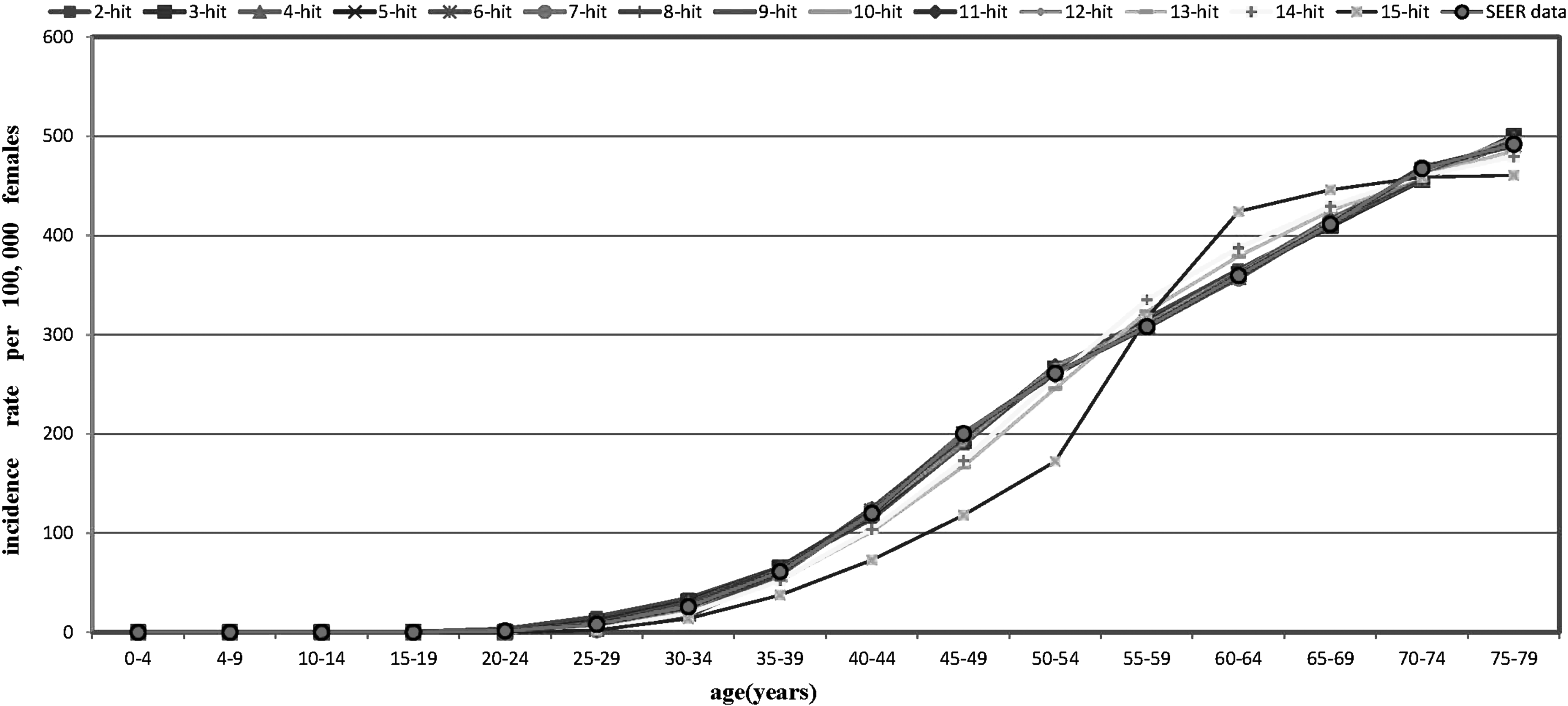
We have only given the optimal fittings for the 2–15-stage models, which are shown in Figure 2. For the models with more than 15 stages, their fitting results are worse than the 15-stage model. From Figure 2, the 2–14-stage models fit the SEER data very well, but the 15-stage model has led to very large error.
The age-specific incidence rates of all races per 100,000 females for breast cancer from the SEER registry for the years 1990–1999 and rates predicted by the 2–15-stage models. SEER, surveillance, epidemiology, and end result.
3.2. Chi-square test of goodness of fit
We use statistical inference to test whether the optimal fittings for 2–14-stage models are available. The chi-square test is chosen to examine those optimal fittings, since the distribution observed in incidence cases is unknown. However, there are only 15 nonzero SEER data by age 79 years, which is impossible for us to examine those optimal fittings for models with more than five stages. To obtain enough data to implement the chi-square test, data set for incidence rate can be converted into data set for probability of breast cancer by the following formula:
\documentclass{aastex}\usepackage{amsbsy}\usepackage{amsfonts}\usepackage{amssymb}\usepackage{bm}\usepackage{mathrsfs}\usepackage{pifont}\usepackage{stmaryrd}\usepackage{textcomp}\usepackage{portland, xspace}\usepackage{amsmath, amsxtra}\usepackage{upgreek}\pagestyle{empty}\DeclareMathSizes{10}{9}{7}{6}\begin{document}
\begin{align*}
P ( t ) = 1 - e{ \rm{xp}} \{ \int_0^t {h ( s ) ds} \} , \tag{15}
\end{align*}
\end{document}
where \documentclass{aastex}\usepackage{amsbsy}\usepackage{amsfonts}\usepackage{amssymb}\usepackage{bm}\usepackage{mathrsfs}\usepackage{pifont}\usepackage{stmaryrd}\usepackage{textcomp}\usepackage{portland, xspace}\usepackage{amsmath, amsxtra}\usepackage{upgreek}\pagestyle{empty}\DeclareMathSizes{10}{9}{7}{6}\begin{document}
$$h ( s )$$
\end{document} denotes the incidence rate of breast cancer at age s. When \documentclass{aastex}\usepackage{amsbsy}\usepackage{amsfonts}\usepackage{amssymb}\usepackage{bm}\usepackage{mathrsfs}\usepackage{pifont}\usepackage{stmaryrd}\usepackage{textcomp}\usepackage{portland, xspace}\usepackage{amsmath, amsxtra}\usepackage{upgreek}\pagestyle{empty}\DeclareMathSizes{10}{9}{7}{6}\begin{document}
$$P ( t )$$
\end{document} is amplified by using a suitable multiple (i.e., 103), there are 49 data points that are >1, which is adequate for performing the chi-square test. The value of the chi-square statistics is determined by
\documentclass{aastex}\usepackage{amsbsy}\usepackage{amsfonts}\usepackage{amssymb}\usepackage{bm}\usepackage{mathrsfs}\usepackage{pifont}\usepackage{stmaryrd}\usepackage{textcomp}\usepackage{portland, xspace}\usepackage{amsmath, amsxtra}\usepackage{upgreek}\pagestyle{empty}\DeclareMathSizes{10}{9}{7}{6}\begin{document}
\begin{align*}
Chi2 = \mathop \sum \limits_{i = 31}^{79} { ( {P_i} - P_i^* ) ^2} * {10^3} / P_i^* , \tag{16}
\end{align*}
\end{document}
where Pi and \documentclass{aastex}\usepackage{amsbsy}\usepackage{amsfonts}\usepackage{amssymb}\usepackage{bm}\usepackage{mathrsfs}\usepackage{pifont}\usepackage{stmaryrd}\usepackage{textcomp}\usepackage{portland, xspace}\usepackage{amsmath, amsxtra}\usepackage{upgreek}\pagestyle{empty}\DeclareMathSizes{10}{9}{7}{6}\begin{document}
$$P_i^*$$
\end{document} are the probability of breast cancer derived from the real data and numerical simulations, respectively.
Table 1 gives the chi-square values calculated using the mentioned equation and values at the 5% significant level for the 2–15-stage models. We find that the chi-square values of the 2–14-stage models are less than the values at the 5% significant level, whereas the chi-square value of the 15-stage model is far larger than the value at the 5% significant level. These suggest that the 2–14 mutations are reasonable for normal breast stem cells to become a malignant cell. In addition, the chi-square values of the three-stage model are the smallest in all models. Thus, the optimal model is the model with three mutations for breast cancer.
The Chi-Square Values Between the Probability Calculated by the Surveillance, Epidemiology, and End Result Data and the Estimated Probability by the Mathematical Models
Chi-square test
2-stage
3-stage
4-stage
5-stage
6-stage
7-stage
8-stage
Chi2
10.191
0.724
1.349
4.433
10.357
9.046
6.2136
df
44
41
38
35
32
29
26
S.5%
60.481
56.942
53.384
49.802
46.194
42.557
38.885
Chi-square test
9-stage
10-stage
11-stage
12-stage
13-stage
14-stage
15-stage
Chi2
18.492
18449
16.451
19.056
16.339
13.790
51.406
df
23
20
17
14
11
8
5
S.5%
35.172
31.410
27.587
23.685
19.675
15.507
11.070
Chi2 denotes the value of chi-square statistic; df ( = 49-1-number of parameters) denotes the degrees of freedom; S.5% denotes the value at 5% significant level.
3.3. Parameter analysis
Table 2 shows the estimated parameter values of the optimal model. The net proliferation rates of intermediate cells with one mutation approach zero. It may be explained by the fact that normal breast stem cells need two mutations in tumor suppressor genes to become the intermediate cells that expand clonally to destroy the homeostasis of cells, or the first mutation occurs in genetic instability genes. Mutations in genetic instability genes increase the rate of mutational processes such as gene amplification, chromosome rearrangements, and gain or loss of whole chromosomes (Lengauer et al., 1998). By comparing the values of \documentclass{aastex}\usepackage{amsbsy}\usepackage{amsfonts}\usepackage{amssymb}\usepackage{bm}\usepackage{mathrsfs}\usepackage{pifont}\usepackage{stmaryrd}\usepackage{textcomp}\usepackage{portland, xspace}\usepackage{amsmath, amsxtra}\usepackage{upgreek}\pagestyle{empty}\DeclareMathSizes{10}{9}{7}{6}\begin{document}
$${ \beta _i}$$
\end{document} and \documentclass{aastex}\usepackage{amsbsy}\usepackage{amsfonts}\usepackage{amssymb}\usepackage{bm}\usepackage{mathrsfs}\usepackage{pifont}\usepackage{stmaryrd}\usepackage{textcomp}\usepackage{portland, xspace}\usepackage{amsmath, amsxtra}\usepackage{upgreek}\pagestyle{empty}\DeclareMathSizes{10}{9}{7}{6}\begin{document}
$${ \beta ^\prime _{ \rm{i}}}$$
\end{document} (\documentclass{aastex}\usepackage{amsbsy}\usepackage{amsfonts}\usepackage{amssymb}\usepackage{bm}\usepackage{mathrsfs}\usepackage{pifont}\usepackage{stmaryrd}\usepackage{textcomp}\usepackage{portland, xspace}\usepackage{amsmath, amsxtra}\usepackage{upgreek}\pagestyle{empty}\DeclareMathSizes{10}{9}{7}{6}\begin{document}
$$i = 1 , 2$$
\end{document}) in Table 2, we find that the net proliferation rates of cells before age 45 years are larger than those after age 45 years. The values of parameters for the models with more than three mutations and the two-stage model have also similar results (the detailed parameter values are displayed in the Supplementary Table S1). These suggest that menopause can reduce or inhibit clonal expansion of cells.
Estimated Optimal Parameter Values (and 95% Confidence Interval, Evaluated Using Chi-Square Statistics) in the Three-Stage Model with Clonal Expansion for Female
Evidence suggests that there is a mutator phenotype that acts as a mechanism in tumor processes, such as genome instability (Loeb, 1991; Leob et al., 2003). Genome instability generates genetic diversity and can contribute to cancer development. When the stability genes are inactivated, mutations in other genes occur at a higher rate (Vogelstein and Kinzler, 2004). To test the genetic instability, we make a hypothesis that all mutation rates are equal in the models, namely \documentclass{aastex}\usepackage{amsbsy}\usepackage{amsfonts}\usepackage{amssymb}\usepackage{bm}\usepackage{mathrsfs}\usepackage{pifont}\usepackage{stmaryrd}\usepackage{textcomp}\usepackage{portland, xspace}\usepackage{amsmath, amsxtra}\usepackage{upgreek}\pagestyle{empty}\DeclareMathSizes{10}{9}{7}{6}\begin{document}
$${ \mu _0} = { \mu _1} = \cdots = { \mu _k}$$
\end{document}. Our results show that only the models with two and three stages can fit the SEER data, whereas the models with more than three stages cannot fit the SEER data. In Figure 3, we plot the hazards for the models with two to four stages under this hypothesis. Thus, there is a mutator phenotype in the tumorigenesis of breast cancer.
The age-specific incidence rates of all races per 100,000 females for breast cancer from the SEER registry for the years 1990–1999 and rates predicted by the two to four-stage models under the hypothesis that all mutation rates are equal.
4. Discussion
Our results suggest that there are 2–14 mutations in the genome of breast stem cells to become a malignant cell, which supports the results of Wood et al. (2007). Using our previous simulation for the data of breast cancer in women carrying germline BRCA1 and BRCA2 mutations, two gene mutations are required in the development of breast cancer (Simon and Zhang, 2008). The model with one mutation cannot fit the data of breast cancer in women carrying germline BRCA1 and BRCA2 mutations. Therefore, there are at least two somatic mutations such that a normal breast stem cell becomes a malignant cell in the genome of breast stem cell. Two to 14 genes are required to be involved in the genetic network for human breast cancer. These conclusions are useful for simplifying the interpretation of individual cancer genomes and the design of future breast cancer genome-sequencing efforts.
There is a mutator phenotype in the tumorigenesis of breast cancer, which can be explained by the genetic instability. The genetic instability is an early event of human cancer, which can be used as the early diagnosis of breast cancer (Lengauer et al., 1998; Zhang and Simon, 2005). Three gene mutations are more likely to occur in the progression of breast cancer. Two mutations are required to destroy the homeostasis of cells in this optimal model. Using the estimated parameter values in the models, we find that the clonal expansion of premalignant cells has an intense relationship with the hormone expression level of females. Menopause can reduce the growth of intermediate cells. Therefore, hormone therapy such as tamoxifen should be effective for breast cancer patients before their menopause.
To explain that many mutations are observed in malignant tumor cells, Loeb et al. (2003) proposed that there is a mutator phenotype that acts as a mechanism in tumor processes. However, Tomlinson and Bodmer (1999) have challenged the mutator phenotype hypothesis and claimed that selection for clonal expansion of intermediate cells is sufficient in tumor processes. This is the general debate for the relationship between mutation and selection. Our results indicate that there is a mutator phenotype in the tumorigenesis of breast cancer. Recent evidence indicates that epigenetic changes might “addict” cancer cells to altered signal transduction pathways during the early stages of tumor development (Klutstein et al., 2016; Herbst et al., 2017). However, epigenetic changes and genomic alterations cannot be easily identified. These findings can provide the guide to the analyses of genes.
Footnotes
Acknowledgments
This research was partially supported by the National Nature Science Foundation of China (Grant Nos. 11071275 and 11371161) and by self-determined research funds of CCNU from the colleges' basic research and operation of MOE (Grant No. CCNU16JCZX10).
Author Disclosure Statement
No competing financial interests exist.
References
1.
ArmitageP., and DollR.1954. The age distribution of cancer and a multi-stage theory of carcinogenesis. Br. J. Cancer, 8, 1–12.
2.
BrouwerA.F., EisenbergM.C., and MezaR.2016. Age effects and temporal trends in HPV-related and HPV-unrelated oral cancer in the United States a multistage carcinogenesis modeling analysis. PLoS One, 11, e0151098.
3.
BrouwerA.F., MezaR., and EisenbergM.C.2016. A systematic approach to determining the identifiability of multistage carcinogenesis models. Risk Anal. 37, 1375–1387.
4.
CrumpK.S., SubramaniamR.P., and Van LandinghamC.B.2005. A numerical solution to the nonhomogeneous two-stage MVK model of cancer. Risk Anal. 25, 921–926.
5.
CurtiusK., HazeltonW.D., JeonJ., et al.2015. A multiscale model evaluates screening for neoplasia in Barrett's Esophagus. PLoS Comput. Biol. 11, e1004272.
6.
EidemüllerM., HolmbergE., JacobP., et al.2015. Breast cancer risk and possible mechanisms of radiation-induced genomic instability in the Swedish hemangioma cohort after reanalyzed dosimetry. Mutat. Res., 775, 1–9.
7.
HanahanD., and WeinbergR.A.2011. The hallmarks of cancer: The next generation. Cell, 144, 646–674.
8.
HarrisT.E.1963. The Theory of Branching Processes. Prentice-Hall Applied Mathematics Series, Englewood Cliffs, NJ.
9.
HazeltonW.D., CurtiusK., InadomiJ.M., et al.2015. The role of gastroesophageal reflux and other factors during progression to esophageal adenocarcinoma. Cancer Epidemiol. Biomarkers Prev., 24, 1012–1023.
10.
HeidenreichW.F., LuebeckE.G., and MoolgavkarS.H.1997. Some properties of the hazard function of the two-mutation clonal expansion model. Risk Anal. 17, 391–399.
11.
HerbstA., VdovinN., GacesaS., et al.2017. Methylated free-circulating HPP1 DNA is an early response marker in patients with metastatic colorectal cancer. Int. J. Cancer, 140, 2134–2144.
12.
JeonJ., LuebeckE.G., and MoolgavkarS.H.2006. Age effects and temporal trends in adenocarcinoma of the esophagus and gastric cardia (United States). Cancer Causes Control, 17, 971–981.
13.
KlutsteinM., NejmanD., GreenfieldR., et al.2016. DNA methylation in cancer and aging. Cancer Res. 76, 3446–3450.
14.
KnudsonA.G.1971. Mutation and cancer: Statistical study of retinoblastoma. Proc. Natl. Acad. Sci. USA, 68, 820–823.
15.
KnudsonA.G.2001. Two genetic hits (more or less) to cancer. Nat. Rev. Cancer, 1, 157–162.
16.
LengauerC., KinzlerK.W., and VogelsteinB.1998. Genetic instabilities in human cancers. Nature, 396, 643–649.
17.
LoebL.A.1991. Mutator phenotype may be required for multistage carcinogenesis. Cancer Res. 51, 3075–3079.
18.
LeobL.A., LoebK.R., and AndersonJ.P.2003. Multiple mutations and cancer. Proc. Natl. Acad. Sci. USA, 100, 776–781.
19.
LuebeckE.G., and MoolgavkarS.H.2002. Multistage carcinogenesis and the incidence of colorectal cancer. Proc. Natl. Acad. Sci. USA, 99, 15095–15100.
20.
MezaR., JeonJ., MoolgavkarS.H., et al.2008. Age-specific incidence of cancer: Phases, transitions, and biological implications. Proc. Natl. Acad. Sci. USA, 105, 16284–16289.
21.
MoolgavkarS.H., DayN.E., and StevensR.G.1980. Two-stage model for carcinogenesis: Epidemiology of breast cancer in females. J. Natl. Cancer Inst., 65, 559–569.
22.
MoolgavkarS.H., HolfordT.R., LevyD.T., et al.2012. Impact of reduced tobacco smoking on lung cancer mortality in the United States during 1975–2000. J. Natl. Cancer Inst., 104, 541–548.
23.
MoolgavkarS.H., and LuebeckG.1990. Two-event model for carcinogenesis: Biological, mathematical, and statistical considerations. Risk Anal. 10, 323–341.
24.
RadmacherM.D., and SimonR.2000. Estimation of Tamoxifen's efficiency for preventing the formation and growth of breast tumors. J. Natl. Cancer Inst., 92, 48–53.
25.
RiesL.A.G., EisnerM.P., KosaryC.L., et al.2002. SEER Cancer Statistics Review, 1973–1999. National Cancer Institute, Bethesda, MD.
26.
SimonR., and ZhangX.2008. On the dynamics of breast tumor development in women carrying germline BRCA1 and BRCA2 mutations. Int. J. Cancer, 122, 1916–1917.
27.
TomasettiC., MarchionniL., NowakM.A., et al.2015. Only three driver gene mutations are required for the development of lung and colorectal cancers. Proc. Natl. Acad. Sci. USA, 112, 118–123.
28.
TomlinsonI.P., and BodmerW.1999. Selection, the mutation rate and cancer: Ensuring that the tail does not wag the dog. Nat. Med., 5, 11–12.
29.
VogelsteinB., and KinzlerK.W.2004. Cancer genes and the pathways they control. Nat. Med., 10, 789–799.
30.
WoodL.D., ParsonsD.W., JonesS., et al.2007. The genomic landscapes of human breast and colorectal cancers. Science, 318, 1108–1113.
31.
ZhangX., FangY., ZhaoY., et al.2014. Mathematical modeling the pathway of human breast cancer. Math. Biosci., 253, 25–29.
32.
ZhangX., and SimonR.2005. Estimating the number of rate limiting genomic changes for human breast cancer. Breast Cancer Res. Treat., 91, 121–124.
Supplementary Material
Please find the following supplemental material available below.
For Open Access articles published under a Creative Commons License, all supplemental material carries the same license as the article it is associated with.
For non-Open Access articles published, all supplemental material carries a non-exclusive license, and permission requests for re-use of supplemental material or any part of supplemental material shall be sent directly to the copyright owner as specified in the copyright notice associated with the article.