A Method for Predicting Protein Complexes from Dynamic Weighted Protein

Abstract

Predicting protein complexes from protein–protein interaction (PPI) network is of great significance to recognize the structure and function of cells. A protein may interact with different proteins under different time or conditions. Existing approaches only utilize static PPI network data that may lose much temporal biological information. First, this article proposed a novel method that combines gene expression data at different time points with traditional static PPI network to construct different dynamic subnetworks. Second, to further filter out the data noise, the semantic similarity based on gene ontology is regarded as the network weight together with the principal component analysis, which is introduced to deal with the weight computing by three traditional methods. Third, after building a dynamic PPI network, a predicting protein complexes algorithm based on “core-attachment” structural feature is applied to detect complexes from each dynamic subnetworks. Finally, it is revealed from the experimental results that our method proposed in this article performs well on detecting protein complexes from dynamic weighted PPI networks.

1. Introduction

Predicting protein complexes from the protein–protein interaction (PPI) networks is a key step in understanding a protein's biological process (BP) and function. Benefiting from the development of high-throughput techniques, millions of protein interaction data are available to construct PPI networks, which leads the computational method of predicting protein complexes to be more valuable and significant.

A PPI network can be regarded as a graph that consists of vertexes and edges, representing proteins and different interactions, respectively (Shih and Parthasarathy, 2012). In the past decade, more and more computational methods of detecting protein complexes from PPI networks have been proposed (Price et al., 2013). These clustering algorithms can be divided into three categories: graph clustering-based method, local density method, and hierarchical clustering method. King et al. (2012) proposed an algorithm—restricted neighborhood search clustering (RNSC), which is based on classical graph clustering. But the experimental results of RNSC are greatly affected by the parameters. Srihari et al. (2010) proposed another typical graph cluster method—Markov Clustering, which simulates random walking in a PPI network to find protein complexes. Spirin (2004) confirms that, by analyzing the structure of PPI network, protein complexes are related to the density and the connectivity of a local module. The better connectivity of a subgraph means that it may be a complex. From the view mentioned previously, molecular complex detection (MCODE) was presented by Bader and Hogue (2003). And to improve the accuracy (Acc), DPClus (Shigehiko et al., 2006) made a change to the stopping condition for cluster formation, which replaces vertex weight with cluster density. Palla et al. (2007) presented clique percolation method to merge all full connected graphs with k-1 common nodes. Girvan and Newman (2001) provided a method, a typical presentation for hierarchical clustering, based on removing the edges with the highest betweenness.

The false positive and false negative data provided by high-throughput techniques will play a negative role during identifying protein complexes (Kouhsar et al., 2016). So how to deal with the data is also an essential problem. In the past years, many methods are proposed to eliminate the data noise by constructing the weighted PPI networks (Liu et al., 2009; Price et al., 2013). Traditional methods of computing the weight mainly regards the topology information of PPI networks as the edge weights, such as the degree of vertex, average degree, or the density of graph. However, only considering topology information will lead to ignore and lose a lot of biological information. To take the biological information into account, domain–domain interaction information has been introduced (Hayashida et al., 2011).

In the past few years, gene ontology (GO) annotations have been introduced and accepted, because it improved the accuracy of predicting. GO is composed of three domains: BP, molecular functions (MFs), and cellular components (CCs). GO and annotations of GO are often applied to compute the semantic similarity as the weight between two different proteins (Wang et al., 2011). GO is modeled as a directed acyclic graph that represents biological knowledge and the relationship among different genes or the gene product. The higher the score of semantic similarity between two different proteins is, the more possible an interaction of these two proteins will be. The mature semantic similarity methods can be grouped into four categories (Price et al., 2013): (1) path length-based methods, they compute the semantic similarity by observing the path length or the depth to the common ancestor term of different two GO terms in the ontology structure; (2) information content-based methods, the GO annotations express a lot of information about the corresponding gene or the gene product, so the more common a couple of GO annotations are, the more similar the annotations' product is; (3) common term-based methods, they measure the repeat parts between two ancestor term sets; and (4) hybrid methods, integrating the mentioned three methods, hybrid methods incorporate two or more different categories.

The algorithms of detecting protein complexes already mentioned are focused on the static networks. In fact, the relationship of any two different proteins is not immutable, which means that a protein might interact with different proteins under different conditions. It pointed out that a protein may interact with different proteins in different stages of a cell cycle to perform a completely different protein complex (Wang et al., 2013). Because the static networks lost much temporal biological information that reduces the Acc of predicting protein complexes, many researchers realized that we should pay more attention to the dynamic networks instead of the static networks (Chen et al., 2014). Combining the PPI networks data with gene expression data has become a popular approach to construct dynamic networks. The easiest method of processing expression data just chooses the average value of all proteins' gene expression value as a benchmark; if an expression value is higher than the benchmark, the protein is activated at the time point. But this method is rarely applied, because the expression values of different proteins at different time points vary vastly, in addition to that, there is also inevitable background noise associated with the expression value, so the benchmark is hard to be calculated. Another classical algorithm is three-sigma that is proposed by Wang et al. (2011). But these proteins with low expression level will be filtered out, which is the disadvantage of three-sigma.

To reveal the dynamics of PPI network and boost the Acc rate, this article mainly focuses on the following aspects:

1. Integrating expression data and static interaction data that come from high-throughput experiments to construct the dynamic PPI networks.

2. Introducing GO semantic similarity as the weight to filter out the data noise.

3. Proposing a method based on “core-attachment” structure to predict protein complexes.

2. Methods

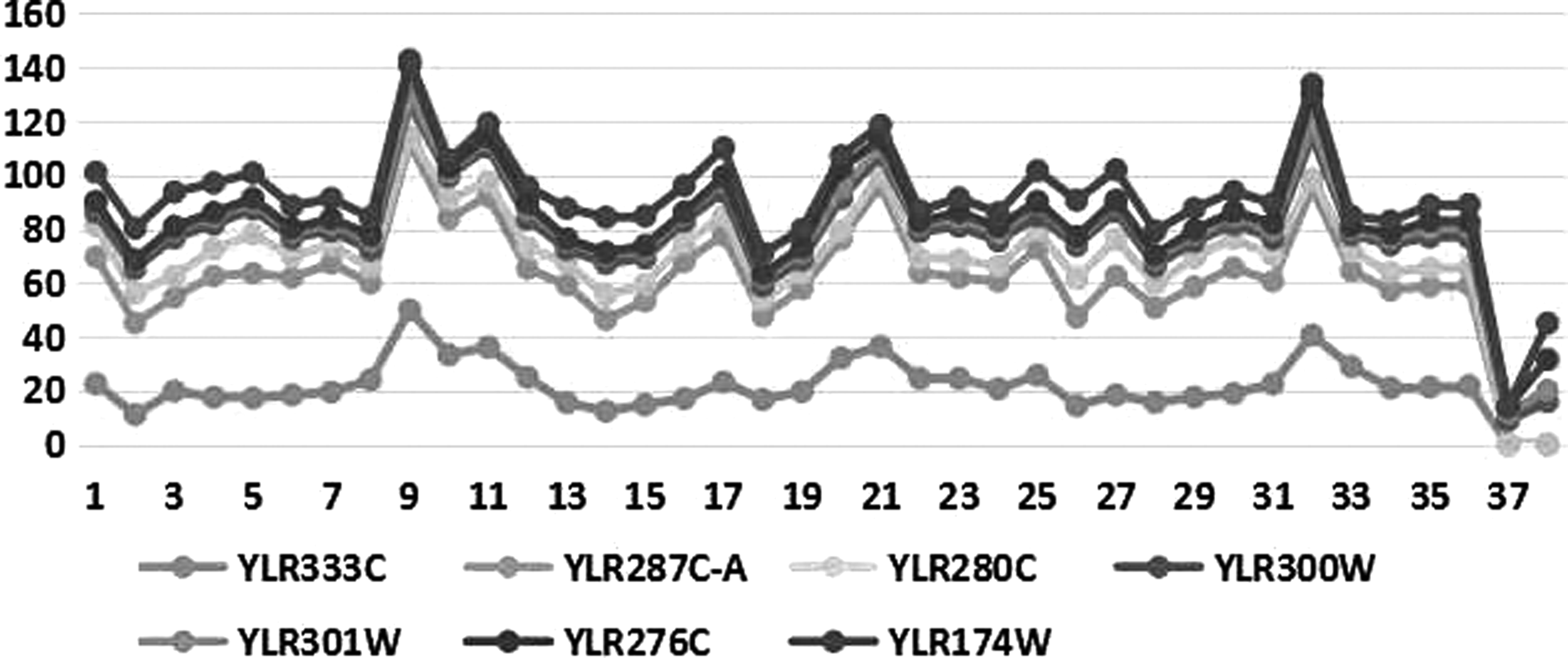
Figure 1 shows the expression activity values among different proteins at different time points. Based on the observation from Figure 1, we can conclude that there is a significant difference among different proteins' expression values. So the important challenge of this research will be, at a particular time point, how to judge whether a protein is active and whether an interaction from the static high-throughput data is valid.

FIG. 1.

Expression values of different proteins at different time points.

The simplest way is using a global threshold to identify the active time point. If the expression value is greater than the threshold, then the protein is active at that time point. But this method does not work well in all situations, (1) because the levels of different proteins vary from protein to protein, there is no global threshold that can suit all proteins and (2) the data are generated by high-throughput experiments that may be embedded with inevitable noise. To construct dynamic networks, Wang et al. (2013) proposed a method called three-sigma to identify active time points of each point. But, the three-sigma method did not work well on the data set with low expression values, such as the YLR332W. This article improves the three-sigma method based on parameter estimation to optimize the variance and mean for each protein.

The number of expression data provided by the experiment method is much smaller than that in a real cellular cycle. So the expression data that we got can be considered as a sample of the population. What we need to do is to estimate the population's variance and mean by those samples. In statistics, we know the interval estimation is often used to calculate the population's variance or mean when the mean or the variance of sample is given. So the interval estimation is introduced to improve the three-sigma algorithm.

2.1. Determine the interval of population's mean and variance

As the expression values of proteins in the static PPI network vary with the time or environment, thus, a static PPI network PN can be broken down into several dynamic networks with smaller size expressed as \documentclass{aastex}\usepackage{amsbsy}\usepackage{amsfonts}\usepackage{amssymb}\usepackage{bm}\usepackage{mathrsfs}\usepackage{pifont}\usepackage{stmaryrd}\usepackage{textcomp}\usepackage{portland, xspace}\usepackage{amsmath, amsxtra}\usepackage{upgreek}\pagestyle{empty}\DeclareMathSizes{10}{9}{7}{6}\begin{document} $$P{N_i}$$ \end{document} , and \documentclass{aastex}\usepackage{amsbsy}\usepackage{amsfonts}\usepackage{amssymb}\usepackage{bm}\usepackage{mathrsfs}\usepackage{pifont}\usepackage{stmaryrd}\usepackage{textcomp}\usepackage{portland, xspace}\usepackage{amsmath, amsxtra}\usepackage{upgreek}\pagestyle{empty}\DeclareMathSizes{10}{9}{7}{6}\begin{document} $$i ( i = 1 , 2 , \cdots 36 )$$ \end{document} is the active time point. So the set PN can be written as \documentclass{aastex}\usepackage{amsbsy}\usepackage{amsfonts}\usepackage{amssymb}\usepackage{bm}\usepackage{mathrsfs}\usepackage{pifont}\usepackage{stmaryrd}\usepackage{textcomp}\usepackage{portland, xspace}\usepackage{amsmath, amsxtra}\usepackage{upgreek}\pagestyle{empty}\DeclareMathSizes{10}{9}{7}{6}\begin{document} $$PN = { \rm{ \{ }}P{N_1} , P{N_{2 , }} \cdots P{N_i} , \cdots P{N_{36}} \} $$ \end{document} , where 36 is the number of time points provided by gene expression data (Wang et al., 2013). For example, in Figure 2, the network PN is a static network, but the other three networks \documentclass{aastex}\usepackage{amsbsy}\usepackage{amsfonts}\usepackage{amssymb}\usepackage{bm}\usepackage{mathrsfs}\usepackage{pifont}\usepackage{stmaryrd}\usepackage{textcomp}\usepackage{portland, xspace}\usepackage{amsmath, amsxtra}\usepackage{upgreek}\pagestyle{empty}\DeclareMathSizes{10}{9}{7}{6}\begin{document} $$P{N_2}$$ \end{document} , \documentclass{aastex}\usepackage{amsbsy}\usepackage{amsfonts}\usepackage{amssymb}\usepackage{bm}\usepackage{mathrsfs}\usepackage{pifont}\usepackage{stmaryrd}\usepackage{textcomp}\usepackage{portland, xspace}\usepackage{amsmath, amsxtra}\usepackage{upgreek}\pagestyle{empty}\DeclareMathSizes{10}{9}{7}{6}\begin{document} $$P{N_6}$$ \end{document} , and \documentclass{aastex}\usepackage{amsbsy}\usepackage{amsfonts}\usepackage{amssymb}\usepackage{bm}\usepackage{mathrsfs}\usepackage{pifont}\usepackage{stmaryrd}\usepackage{textcomp}\usepackage{portland, xspace}\usepackage{amsmath, amsxtra}\usepackage{upgreek}\pagestyle{empty}\DeclareMathSizes{10}{9}{7}{6}\begin{document} $$P{N_{10}}$$ \end{document} are dynamic networks. From this figure, it can be concluded that not all of the proteins are active at all time points.

FIG. 2.

Convert static network into dynamic network at different time points.

Figure 3 illustrates that the expression values vary cyclically every 12 time points. To reduce the time complexity, the expression value of each moment spanning the 12 time points is calculated by the average of three cycles as given in Equation (1). \documentclass{aastex}\usepackage{amsbsy}\usepackage{amsfonts}\usepackage{amssymb}\usepackage{bm}\usepackage{mathrsfs}\usepackage{pifont}\usepackage{stmaryrd}\usepackage{textcomp}\usepackage{portland, xspace}\usepackage{amsmath, amsxtra}\usepackage{upgreek}\pagestyle{empty}\DeclareMathSizes{10}{9}{7}{6}\begin{document} \begin{align*} newValu { e_ { { T_i } } } = \frac { { valu { e_ { { T_i } } } + valu { e_ { { T_ { i + 12 } } } } + valu { e_ { { T_ { i + 24 } } } } } } { 3 } , \tag { 1 } \end{align*} \end{document}

FIG. 3.

Periodic expression among different proteins.

Suppose that samples \documentclass{aastex}\usepackage{amsbsy}\usepackage{amsfonts}\usepackage{amssymb}\usepackage{bm}\usepackage{mathrsfs}\usepackage{pifont}\usepackage{stmaryrd}\usepackage{textcomp}\usepackage{portland, xspace}\usepackage{amsmath, amsxtra}\usepackage{upgreek}\pagestyle{empty}\DeclareMathSizes{10}{9}{7}{6}\begin{document} $${x_1} , {x_2} , \cdots , {x_n}$$ \end{document} are extracted from a population that obeys normal distribution \documentclass{aastex}\usepackage{amsbsy}\usepackage{amsfonts}\usepackage{amssymb}\usepackage{bm}\usepackage{mathrsfs}\usepackage{pifont}\usepackage{stmaryrd}\usepackage{textcomp}\usepackage{portland, xspace}\usepackage{amsmath, amsxtra}\usepackage{upgreek}\pagestyle{empty}\DeclareMathSizes{10}{9}{7}{6}\begin{document} $$N ( \mu , { \sigma ^2} )$$ \end{document} , we can get the following conclusion: \documentclass{aastex}\usepackage{amsbsy}\usepackage{amsfonts}\usepackage{amssymb}\usepackage{bm}\usepackage{mathrsfs}\usepackage{pifont}\usepackage{stmaryrd}\usepackage{textcomp}\usepackage{portland, xspace}\usepackage{amsmath, amsxtra}\usepackage{upgreek}\pagestyle{empty}\DeclareMathSizes{10}{9}{7}{6}\begin{document} \begin{align*} Y = \frac { { ( \mathop x \limits^ - - \mu ) \sqrt n } } { s } \sim t ( n - 1 ) , \tag { 2 } \end{align*} \end{document} \documentclass{aastex}\usepackage{amsbsy}\usepackage{amsfonts}\usepackage{amssymb}\usepackage{bm}\usepackage{mathrsfs}\usepackage{pifont}\usepackage{stmaryrd}\usepackage{textcomp}\usepackage{portland, xspace}\usepackage{amsmath, amsxtra}\usepackage{upgreek}\pagestyle{empty}\DeclareMathSizes{10}{9}{7}{6}\begin{document} \begin{align*} Z = { \frac { ( n - 1 ) { s^2 } } { { \sigma ^2 } } } \sim { \chi ^2 } ( n - 1 ) , \tag { 3 } \end{align*} \end{document}

Under the condition of confidence level \documentclass{aastex}\usepackage{amsbsy}\usepackage{amsfonts}\usepackage{amssymb}\usepackage{bm}\usepackage{mathrsfs}\usepackage{pifont}\usepackage{stmaryrd}\usepackage{textcomp}\usepackage{portland, xspace}\usepackage{amsmath, amsxtra}\usepackage{upgreek}\pagestyle{empty}\DeclareMathSizes{10}{9}{7}{6}\begin{document} $$\alpha = 0.05$$ \end{document} , the maximum possible interval of the mean distribution is shown in Figure 4, which is equal to Equation (4). \documentclass{aastex}\usepackage{amsbsy}\usepackage{amsfonts}\usepackage{amssymb}\usepackage{bm}\usepackage{mathrsfs}\usepackage{pifont}\usepackage{stmaryrd}\usepackage{textcomp}\usepackage{portland, xspace}\usepackage{amsmath, amsxtra}\usepackage{upgreek}\pagestyle{empty}\DeclareMathSizes{10}{9}{7}{6}\begin{document} \begin{align*} p \{ \vert Y \vert \le {t_{{ \alpha \mathord{ \left/ { \vphantom { \alpha 2}} \right. \kern \nulldelimiterspace} 2}}} ( n - 1 ) \} = 1 - \alpha \tag{4} \end{align*} \end{document}

FIG. 4.

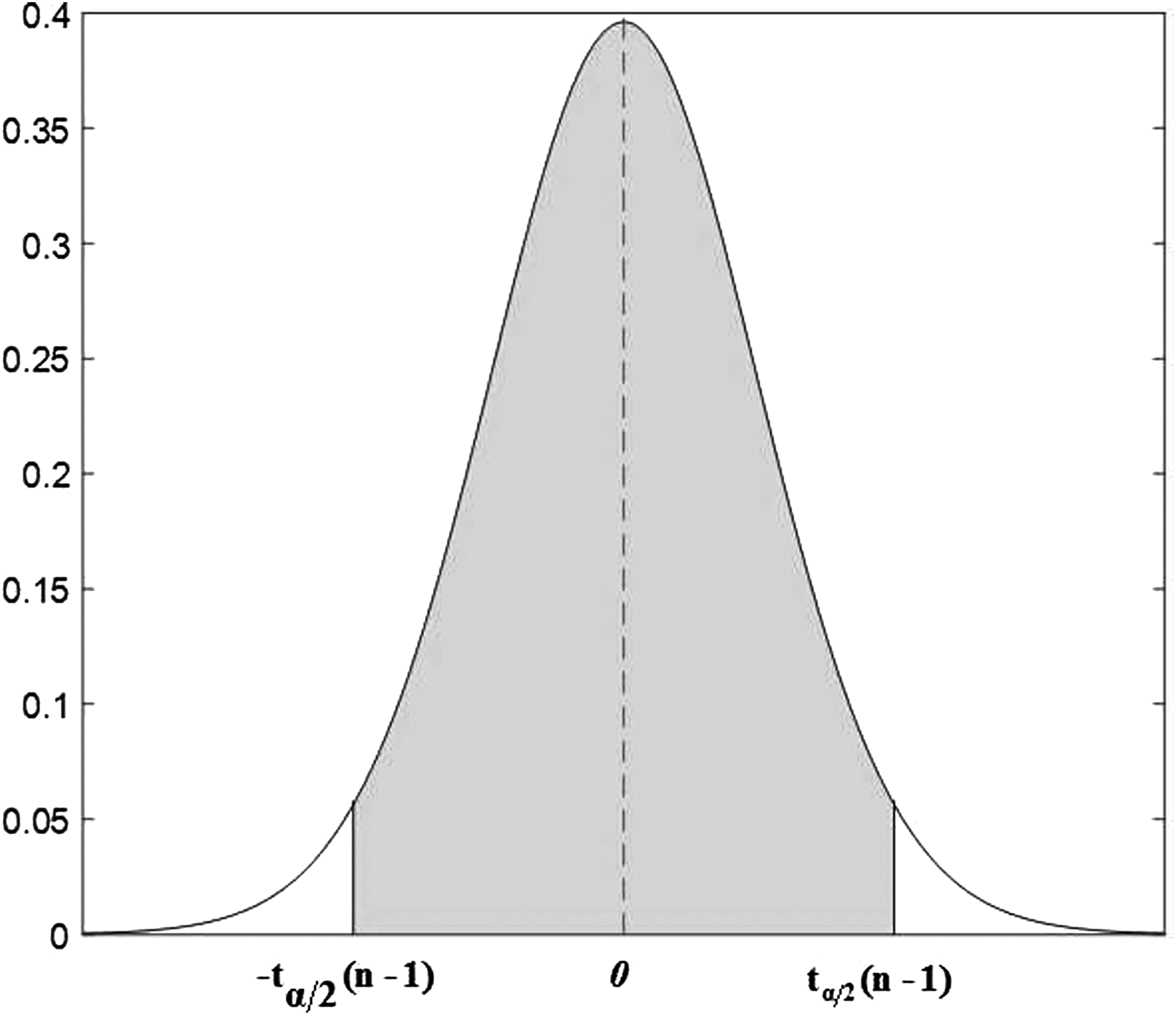
T-distribution function.

Based on Equations (2) and (4), Equation (5) about population's mean can be inferred as follows: \documentclass{aastex}\usepackage{amsbsy}\usepackage{amsfonts}\usepackage{amssymb}\usepackage{bm}\usepackage{mathrsfs}\usepackage{pifont}\usepackage{stmaryrd}\usepackage{textcomp}\usepackage{portland, xspace}\usepackage{amsmath, amsxtra}\usepackage{upgreek}\pagestyle{empty}\DeclareMathSizes{10}{9}{7}{6}\begin{document} \begin{align*} p { \rm { \ { } } \mathop { \rm { x } } \limits^ - - { { \rm { t } } _ { { { \rm { \alpha } } \mathord { \left/ { \vphantom { { \rm { \alpha } } { \rm { 2 } } } } \right. \kern \nulldelimiterspace } { \rm { 2 } } } } } { \rm { ( n } } - { \rm { 1 ) } } { \frac { \rm { s } } { \sqrt { \rm { n } } } } \le { \rm { \mu } } \le \mathop { \rm { x } } \limits^ - + { { \rm { t } } _ { { { \rm { \alpha } } \mathord { \left/ { \vphantom { { \rm { \alpha } } { \rm { 2 } } } } \right. \kern \nulldelimiterspace } { \rm { 2 } } } } } { \rm { ( n } } - { \rm { 1 ) } } { \frac { \rm { s } } { \sqrt { \rm { n } } } } { \rm { \ } } } = { \rm { 1 } } - { { \alpha } } \tag { 5 } \end{align*} \end{document}

So the confidence interval of the population's mean \documentclass{aastex}\usepackage{amsbsy}\usepackage{amsfonts}\usepackage{amssymb}\usepackage{bm}\usepackage{mathrsfs}\usepackage{pifont}\usepackage{stmaryrd}\usepackage{textcomp}\usepackage{portland, xspace}\usepackage{amsmath, amsxtra}\usepackage{upgreek}\pagestyle{empty}\DeclareMathSizes{10}{9}{7}{6}\begin{document} $$\mu$$ \end{document} is \documentclass{aastex}\usepackage{amsbsy}\usepackage{amsfonts}\usepackage{amssymb}\usepackage{bm}\usepackage{mathrsfs}\usepackage{pifont}\usepackage{stmaryrd}\usepackage{textcomp}\usepackage{portland, xspace}\usepackage{amsmath, amsxtra}\usepackage{upgreek}\pagestyle{empty}\DeclareMathSizes{10}{9}{7}{6}\begin{document} \begin{align*} [ \mathop x \limits^ - - { t_ { { \alpha \mathord { \left/ { \vphantom { \alpha 2 } } \right. \kern \nulldelimiterspace } 2 } } } ( n - 1 ) \frac { s } { { \sqrt n } } , \mathop x \limits^ - + { t_ { { \alpha \mathord { \left/ { \vphantom { \alpha 2 } } \right. \kern \nulldelimiterspace } 2 } } } ( n - 1 ) \frac { s } { { \sqrt n } } ] \end{align*} \end{document} .

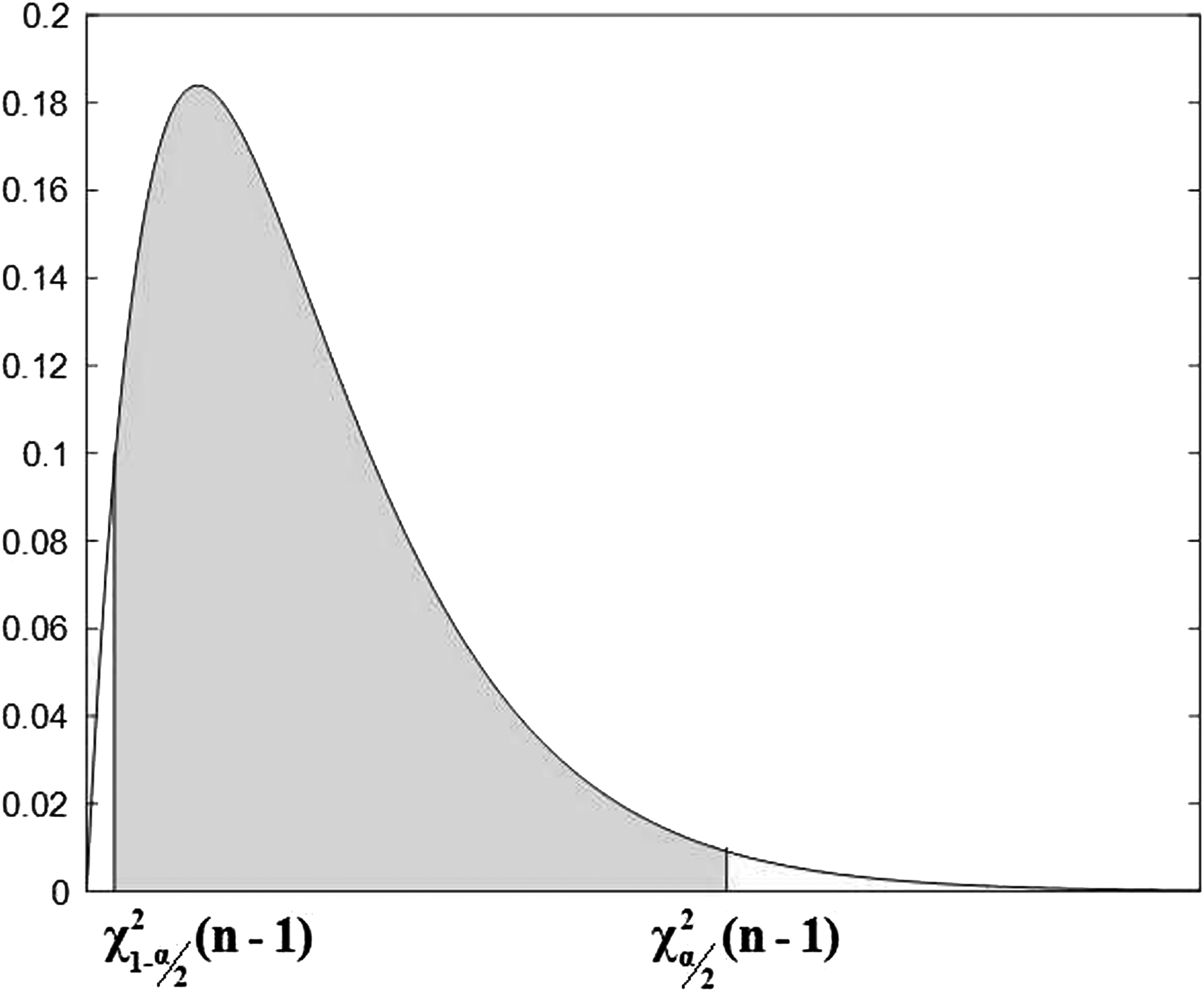
In a similar manner, the maximum possible interval of variance shown in Figure 5 can be written as the mathematical expression as Equation (6). \documentclass{aastex}\usepackage{amsbsy}\usepackage{amsfonts}\usepackage{amssymb}\usepackage{bm}\usepackage{mathrsfs}\usepackage{pifont}\usepackage{stmaryrd}\usepackage{textcomp}\usepackage{portland, xspace}\usepackage{amsmath, amsxtra}\usepackage{upgreek}\pagestyle{empty}\DeclareMathSizes{10}{9}{7}{6}\begin{document} \begin{align*} p\{ \chi _{1 - {\raise0.7ex\hbox{$\alpha $} \!\mathord{\left/ {\vphantom {\alpha 2}}\right.\kern-\nulldelimiterspace} \!\lower0.7ex\hbox{$2$}}}^2(n - 1) \le Z \le \chi _{_{{\alpha \mathord{\left/ {\vphantom {\alpha 2}} \right. \kern-\nulldelimiterspace} 2}}}^2(n - 1)\} = 1 - \alpha \tag { 6 } \end{align*} \end{document}

FIG. 5.

Chi-square distribution function.

Thus, combining Equations (3) and (6), we can get Equation (7). \documentclass{aastex}\usepackage{amsbsy}\usepackage{amsfonts}\usepackage{amssymb}\usepackage{bm}\usepackage{mathrsfs}\usepackage{pifont}\usepackage{stmaryrd}\usepackage{textcomp}\usepackage{portland, xspace}\usepackage{amsmath, amsxtra}\usepackage{upgreek}\pagestyle{empty}\DeclareMathSizes{10}{9}{7}{6}\begin{document} \begin{align*} p \ \frac { { { ( n - 1 ) { s^2 } } { \chi _ { { \alpha \mathord { \left/ { \vphantom { \alpha 2 } } \right. \kern \nulldelimiterspace } 2 } } ^2 ( n - 1 ) } } \le { \sigma ^2 } \le { \frac { ( n - 1 ) { s^2 } } { \chi _ { 1 - { \alpha \mathord { \left/ { \vphantom { \alpha 2 } } \right. \kern \nulldelimiterspace } 2 } } ^2 ( n - 1 ) } } \ } = 1 - \alpha \tag { 7 } \end{align*} \end{document}

In summary, the confidence interval of the population's variance \documentclass{aastex}\usepackage{amsbsy}\usepackage{amsfonts}\usepackage{amssymb}\usepackage{bm}\usepackage{mathrsfs}\usepackage{pifont}\usepackage{stmaryrd}\usepackage{textcomp}\usepackage{portland, xspace}\usepackage{amsmath, amsxtra}\usepackage{upgreek}\pagestyle{empty}\DeclareMathSizes{10}{9}{7}{6}\begin{document} $${ \sigma ^2}$$ \end{document} is \documentclass{aastex}\usepackage{amsbsy}\usepackage{amsfonts}\usepackage{amssymb}\usepackage{bm}\usepackage{mathrsfs}\usepackage{pifont}\usepackage{stmaryrd}\usepackage{textcomp}\usepackage{portland, xspace}\usepackage{amsmath, amsxtra}\usepackage{upgreek}\pagestyle{empty}\DeclareMathSizes{10}{9}{7}{6}\begin{document} \begin{align*} \Big[ { \frac { ( n - 1 ) { s^2 } } { \chi _ { { \alpha \mathord { \left/ { \vphantom { \alpha 2 } } \right. \kern \nulldelimiterspace } 2 } } ^2 ( n - 1 ) } } , { \frac { ( n - 1 ) { s^2 } } { \chi _ { 1 - { \alpha \mathord { \left/ { \vphantom { \alpha 2 } } \right. \kern \nulldelimiterspace } 2 } } ^2 ( n - 1 ) } } \Big] \end{align*} \end{document} .

2.2. Improved three-sigma method

The traditional three-sigma method described as Equation (8) is likely to filter out active proteins with low expression. \documentclass{aastex}\usepackage{amsbsy}\usepackage{amsfonts}\usepackage{amssymb}\usepackage{bm}\usepackage{mathrsfs}\usepackage{pifont}\usepackage{stmaryrd}\usepackage{textcomp}\usepackage{portland, xspace}\usepackage{amsmath, amsxtra}\usepackage{upgreek}\pagestyle{empty}\DeclareMathSizes{10}{9}{7}{6}\begin{document} \begin{align*} Act{\hbox{-}}thr ( p ) = {s_1} ( p ) \times F ( p ) + {s_2} ( p ) \times ( 1 - F ( p ) ) , \tag{8} \end{align*} \end{document}

in which \documentclass{aastex}\usepackage{amsbsy}\usepackage{amsfonts}\usepackage{amssymb}\usepackage{bm}\usepackage{mathrsfs}\usepackage{pifont}\usepackage{stmaryrd}\usepackage{textcomp}\usepackage{portland, xspace}\usepackage{amsmath, amsxtra}\usepackage{upgreek}\pagestyle{empty}\DeclareMathSizes{10}{9}{7}{6}\begin{document} \begin{align*} { s_1 } ( p ) = \mu ( p ) , \ { s_2 } = \mu ( p ) + 3 \sigma ( p ) , \ F ( p ) = \frac { 1 } { { 1 + { \sigma ^2 } ( p ) } } \end{align*} \end{document} , and p represents a kind of protein.

From Equation (8), it is observed that the active threshold depends on the mean and variance. A protein with low expression value at most time points, such as YLR331C, will be filtered out incorrectly according to this formula. To solve this problem, this article makes some improvements on \documentclass{aastex}\usepackage{amsbsy}\usepackage{amsfonts}\usepackage{amssymb}\usepackage{bm}\usepackage{mathrsfs}\usepackage{pifont}\usepackage{stmaryrd}\usepackage{textcomp}\usepackage{portland, xspace}\usepackage{amsmath, amsxtra}\usepackage{upgreek}\pagestyle{empty}\DeclareMathSizes{10}{9}{7}{6}\begin{document} $$\mu ( p )$$ \end{document} and \documentclass{aastex}\usepackage{amsbsy}\usepackage{amsfonts}\usepackage{amssymb}\usepackage{bm}\usepackage{mathrsfs}\usepackage{pifont}\usepackage{stmaryrd}\usepackage{textcomp}\usepackage{portland, xspace}\usepackage{amsmath, amsxtra}\usepackage{upgreek}\pagestyle{empty}\DeclareMathSizes{10}{9}{7}{6}\begin{document} $$\sigma ( p )$$ \end{document} , as shown in Equation (9). \documentclass{aastex}\usepackage{amsbsy}\usepackage{amsfonts}\usepackage{amssymb}\usepackage{bm}\usepackage{mathrsfs}\usepackage{pifont}\usepackage{stmaryrd}\usepackage{textcomp}\usepackage{portland, xspace}\usepackage{amsmath, amsxtra}\usepackage{upgreek}\pagestyle{empty}\DeclareMathSizes{10}{9}{7}{6}\begin{document} \begin{align*} { \mathop{ \rm Im} \nolimits} p - act ( p ) = S_1^ \prime ( p ) \times F ( p ) + S_2^ \prime ( p ) \times ( 1 - F ( p ) ) , \tag{9} \end{align*} \end{document}

where \documentclass{aastex}\usepackage{amsbsy}\usepackage{amsfonts}\usepackage{amssymb}\usepackage{bm}\usepackage{mathrsfs}\usepackage{pifont}\usepackage{stmaryrd}\usepackage{textcomp}\usepackage{portland, xspace}\usepackage{amsmath, amsxtra}\usepackage{upgreek}\pagestyle{empty}\DeclareMathSizes{10}{9}{7}{6}\begin{document} $$ { \mu ^ \prime } = \mathop x \limits^ - - { t_ { { \alpha \mathord { \left/ { \vphantom { \alpha 2 } } \right. \kern \nulldelimiterspace } 2 } } } ( n - 1 ) \frac { s } { { \sqrt n } } + d \times { \frac { \max ( \exp ( p ) ) - \min ( \exp ( p ) ) } { 36 } }$$ \end{document} and \documentclass{aastex}\usepackage{amsbsy}\usepackage{amsfonts}\usepackage{amssymb}\usepackage{bm}\usepackage{mathrsfs}\usepackage{pifont}\usepackage{stmaryrd}\usepackage{textcomp}\usepackage{portland, xspace}\usepackage{amsmath, amsxtra}\usepackage{upgreek}\pagestyle{empty}\DeclareMathSizes{10}{9}{7}{6}\begin{document} \begin{align*}{ \sigma ^ { \prime 2 } } = { \frac { ( n - 1 ) { s^2 } } { \chi _ { { \alpha \mathord { \left/ { \vphantom { \alpha 2 } } \right. \kern \nulldelimiterspace } 2 } } ^2 ( n - 1 ) } } + d \times { \frac { \max ( \exp ( p ) ) - \min ( \exp ( p ) ) } { 36 } }\end{align*} \end{document} , \documentclass{aastex}\usepackage{amsbsy}\usepackage{amsfonts}\usepackage{amssymb}\usepackage{bm}\usepackage{mathrsfs}\usepackage{pifont}\usepackage{stmaryrd}\usepackage{textcomp}\usepackage{portland, xspace}\usepackage{amsmath, amsxtra}\usepackage{upgreek}\pagestyle{empty}\DeclareMathSizes{10}{9}{7}{6}\begin{document} $$\exp ( p )$$ \end{document} is the expression value of protein p, d is a parameter to adjust the mean or the variance of a protein in the range of its confidence interval, and \documentclass{aastex}\usepackage{amsbsy}\usepackage{amsfonts}\usepackage{amssymb}\usepackage{bm}\usepackage{mathrsfs}\usepackage{pifont}\usepackage{stmaryrd}\usepackage{textcomp}\usepackage{portland, xspace}\usepackage{amsmath, amsxtra}\usepackage{upgreek}\pagestyle{empty}\DeclareMathSizes{10}{9}{7}{6}\begin{document} $$ \mathop x \limits^ - - { t_ { { \alpha \mathord { \left/ { \vphantom { \alpha 2 } } \right. \kern \nulldelimiterspace } 2 } } } ( n - 1 ) \frac { s } { { \sqrt n } }$$ \end{document} is the low boundary of mean's confidence interval. Similarly, \documentclass{aastex}\usepackage{amsbsy}\usepackage{amsfonts}\usepackage{amssymb}\usepackage{bm}\usepackage{mathrsfs}\usepackage{pifont}\usepackage{stmaryrd}\usepackage{textcomp}\usepackage{portland, xspace}\usepackage{amsmath, amsxtra}\usepackage{upgreek}\pagestyle{empty}\DeclareMathSizes{10}{9}{7}{6}\begin{document} $$ { \frac { ( n - 1 ) { s^2 } } { \chi _ { { \alpha \mathord { \left/ { \vphantom { \alpha 2 } } \right. \kern \nulldelimiterspace } 2 } } ^2 ( n - 1 ) } }$$ \end{document} is the low boundary of variance's confidence interval. If at a certain time point, a protein's expression value \documentclass{aastex}\usepackage{amsbsy}\usepackage{amsfonts}\usepackage{amssymb}\usepackage{bm}\usepackage{mathrsfs}\usepackage{pifont}\usepackage{stmaryrd}\usepackage{textcomp}\usepackage{portland, xspace}\usepackage{amsmath, amsxtra}\usepackage{upgreek}\pagestyle{empty}\DeclareMathSizes{10}{9}{7}{6}\begin{document} $$\exp ( {p_i} )$$ \end{document} is lower than \documentclass{aastex}\usepackage{amsbsy}\usepackage{amsfonts}\usepackage{amssymb}\usepackage{bm}\usepackage{mathrsfs}\usepackage{pifont}\usepackage{stmaryrd}\usepackage{textcomp}\usepackage{portland, xspace}\usepackage{amsmath, amsxtra}\usepackage{upgreek}\pagestyle{empty}\DeclareMathSizes{10}{9}{7}{6}\begin{document} $${ \mathop{ \rm Im} \nolimits} p - act ( p )$$ \end{document} , then the active probability p_i is 0; in contrast, if \documentclass{aastex}\usepackage{amsbsy}\usepackage{amsfonts}\usepackage{amssymb}\usepackage{bm}\usepackage{mathrsfs}\usepackage{pifont}\usepackage{stmaryrd}\usepackage{textcomp}\usepackage{portland, xspace}\usepackage{amsmath, amsxtra}\usepackage{upgreek}\pagestyle{empty}\DeclareMathSizes{10}{9}{7}{6}\begin{document} $$\exp ( {p_i} )$$ \end{document} is higher than threshold \documentclass{aastex}\usepackage{amsbsy}\usepackage{amsfonts}\usepackage{amssymb}\usepackage{bm}\usepackage{mathrsfs}\usepackage{pifont}\usepackage{stmaryrd}\usepackage{textcomp}\usepackage{portland, xspace}\usepackage{amsmath, amsxtra}\usepackage{upgreek}\pagestyle{empty}\DeclareMathSizes{10}{9}{7}{6}\begin{document} $${ \mathop{ \rm Im} \nolimits} p - act ( p )$$ \end{document} , then p_i is 1. Consequently, the whole dynamic PPI networks can be represented as \documentclass{aastex}\usepackage{amsbsy}\usepackage{amsfonts}\usepackage{amssymb}\usepackage{bm}\usepackage{mathrsfs}\usepackage{pifont}\usepackage{stmaryrd}\usepackage{textcomp}\usepackage{portland, xspace}\usepackage{amsmath, amsxtra}\usepackage{upgreek}\pagestyle{empty}\DeclareMathSizes{10}{9}{7}{6}\begin{document} $$act - ne{t_i}$$ \end{document} : \documentclass{aastex}\usepackage{amsbsy}\usepackage{amsfonts}\usepackage{amssymb}\usepackage{bm}\usepackage{mathrsfs}\usepackage{pifont}\usepackage{stmaryrd}\usepackage{textcomp}\usepackage{portland, xspace}\usepackage{amsmath, amsxtra}\usepackage{upgreek}\pagestyle{empty}\DeclareMathSizes{10}{9}{7}{6}\begin{document} \begin{align*} act - ne{t_i} = {P_i} \cdot P_i^T , \end{align*} \end{document}

where P_i is a column vector about the active probability of all proteins at time point i, and \documentclass{aastex}\usepackage{amsbsy}\usepackage{amsfonts}\usepackage{amssymb}\usepackage{bm}\usepackage{mathrsfs}\usepackage{pifont}\usepackage{stmaryrd}\usepackage{textcomp}\usepackage{portland, xspace}\usepackage{amsmath, amsxtra}\usepackage{upgreek}\pagestyle{empty}\DeclareMathSizes{10}{9}{7}{6}\begin{document} $$P_i^T$$ \end{document} is the transposition of P_i.

2.3. GO semantic similarity

As a measure of filtering out data noise, weighted network has become more essential. Among these proposed approaches, topological information (Li et al., 2012) is the first applied method. However, the weight of a protein interaction does not only depend on the topological structure but also relies on the biological information. Ozawa et al. (2010) and Ma et al. (2012) applied the domain interaction information into constructing a weighted PPI network and confirmed that the bioinformatics plays a pivotal role in predicting protein complexes. At the meantime, more researchers tend to look favorably on GO semantic similarity, which is a function computing closeness in meaning between terms with an ontology in the past few years. Three approaches that are Jiang and Conrath (1997), Lin (1998), and SimGIC (Lu et al., 2012) are adopted in this article to calculate the semantic similarity.

These three semantic similarity measures contribute from different perspectives: to integrate the different information and remove redundant information, principal component analysis (PCA) is introduced, which is a statistical procedure and its function is to reduce the dimension of the sample feature. The weight of an interaction i in the network computed by different methods can be represented as a vector V_i: \documentclass{aastex}\usepackage{amsbsy}\usepackage{amsfonts}\usepackage{amssymb}\usepackage{bm}\usepackage{mathrsfs}\usepackage{pifont}\usepackage{stmaryrd}\usepackage{textcomp}\usepackage{portland, xspace}\usepackage{amsmath, amsxtra}\usepackage{upgreek}\pagestyle{empty}\DeclareMathSizes{10}{9}{7}{6}\begin{document} $${V_i} = ( {J_i} , {L_i} , {S_i} )$$ \end{document} , where \documentclass{aastex}\usepackage{amsbsy}\usepackage{amsfonts}\usepackage{amssymb}\usepackage{bm}\usepackage{mathrsfs}\usepackage{pifont}\usepackage{stmaryrd}\usepackage{textcomp}\usepackage{portland, xspace}\usepackage{amsmath, amsxtra}\usepackage{upgreek}\pagestyle{empty}\DeclareMathSizes{10}{9}{7}{6}\begin{document} $${J_i} , {L_i}$$ \end{document} , and S_i represent the score computed by Jiang and Conrath (1997), Lin (1998), and SimGIC methods. We can consider interaction i as a sample, and the scores computed by Jiang and Conrath (1997), Lin (1998), and SimGIC are the three properties of the sample. Then PCA is used to translate those three properties into one property. The process already mentioned is adopted to deal with BP, MF, and CC, respectively. The last weight between an interaction is the average of those three parts.

Some GO without annotations will influence the construction of weighted PPI network. In this article, the mean of semantic similarity values with annotation will be considered as the weight of interaction without annotation.

So far, we can build a complete network at any time point i. \documentclass{aastex}\usepackage{amsbsy}\usepackage{amsfonts}\usepackage{amssymb}\usepackage{bm}\usepackage{mathrsfs}\usepackage{pifont}\usepackage{stmaryrd}\usepackage{textcomp}\usepackage{portland, xspace}\usepackage{amsmath, amsxtra}\usepackage{upgreek}\pagestyle{empty}\DeclareMathSizes{10}{9}{7}{6}\begin{document} \begin{align*} DI{N_i} = act - ne{t_i} \circ {W_i} , \end{align*} \end{document}

where w_i is the weight matrix and \documentclass{aastex}\usepackage{amsbsy}\usepackage{amsfonts}\usepackage{amssymb}\usepackage{bm}\usepackage{mathrsfs}\usepackage{pifont}\usepackage{stmaryrd}\usepackage{textcomp}\usepackage{portland, xspace}\usepackage{amsmath, amsxtra}\usepackage{upgreek}\pagestyle{empty}\DeclareMathSizes{10}{9}{7}{6}\begin{document} $$\circ$$ \end{document} is element-wise multiplication.

2.4. Algorithm of predicting protein complexes

Dezso et al. (2003) and Gavin et al. (2006) pointed out that the structure of a protein complex can be described as a core-attachment as shown in Figure 6, where proteins A, B, C, and D form a group called core, all of the proteins E, F, G, and H are the attachments around the core. By the inspiration of this structure, a novel algorithm called DWCOACH is proposed in this article. The new method mainly contains several subfunctions, including filtering seed proteins, construction of cores, adjunction of attachment proteins, and elimination of redundant protein complexes. Algorithm 1 describes the main process of predicting protein complexes. The static PPI network is regarded as the input, and the protein complexes are the output. Line 3 is to deal with the expression value by using the three-sigma method to shift static PPI network to dynamic PPI network. The main task of lines 4–6 is to compute all the weighted local clustering coefficient, and add the proteins with its clustering coefficient into a set Initial-protein, which will be used in the seed-Generation subfunction to find the seed for the construction of core in line 7. In line 8, the selected seeds and the dynamic subnetworks are used in the other subfunction—core-Construction, to construct a protein group made up of seed proteins as a core of a protein complex. To expand a core, the attachment proteins that satisfy the judgment condition will be added into a core as shown in lines 9–10. Many redundancies are generated from the first 10 lines, so the last thing we need to do is refine the complexes as shown in line 11.

FIG. 6.

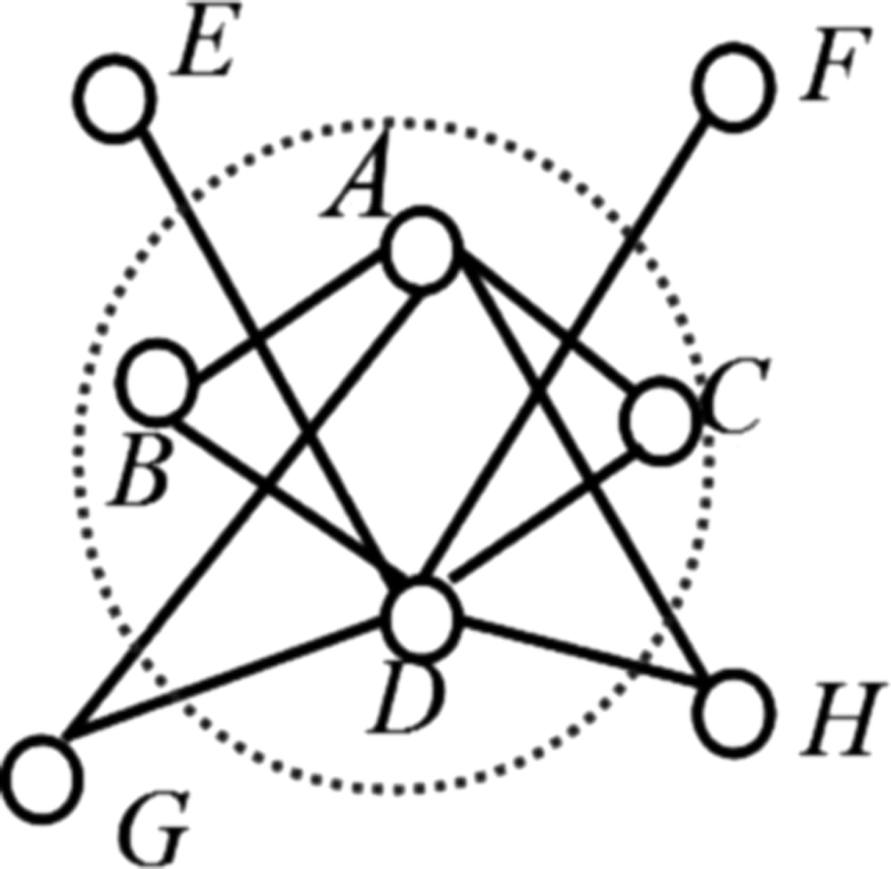
Core-attachment structure.

Algorithm 1: General Framework of DWCOACH
Input: static PPI network SPN
Output: protein complexes
1. Initial-protein = { }
2. complexes = { }
3. PN = threeSigma(SPN)
4. for each protein p_i in dynamic PPI network \documentclass{aastex}\usepackage{amsbsy}\usepackage{amsfonts}\usepackage{amssymb}\usepackage{bm}\usepackage{mathrsfs}\usepackage{pifont}\usepackage{stmaryrd}\usepackage{textcomp}\usepackage{portland, xspace}\usepackage{amsmath, amsxtra}\usepackage{upgreek}\pagestyle{empty}\DeclareMathSizes{10}{9}{7}{6}\begin{document} $$P{N_j}$$ \end{document} :
5. Initial-protein.add( \documentclass{aastex}\usepackage{amsbsy}\usepackage{amsfonts}\usepackage{amssymb}\usepackage{bm}\usepackage{mathrsfs}\usepackage{pifont}\usepackage{stmaryrd}\usepackage{textcomp}\usepackage{portland, xspace}\usepackage{amsmath, amsxtra}\usepackage{upgreek}\pagestyle{empty}\DeclareMathSizes{10}{9}{7}{6}\begin{document} $${p_i} , CC ( {p_i} ) )$$ \end{document} )
6. end for
7. seed = seed-Generation(Initial-protein)
8. core = core-Construction(seed, \documentclass{aastex}\usepackage{amsbsy}\usepackage{amsfonts}\usepackage{amssymb}\usepackage{bm}\usepackage{mathrsfs}\usepackage{pifont}\usepackage{stmaryrd}\usepackage{textcomp}\usepackage{portland, xspace}\usepackage{amsmath, amsxtra}\usepackage{upgreek}\pagestyle{empty}\DeclareMathSizes{10}{9}{7}{6}\begin{document} $$P{N_j}$$ \end{document} )
9. complex = attachment(core)
10. complexes = complexes \documentclass{aastex}\usepackage{amsbsy}\usepackage{amsfonts}\usepackage{amssymb}\usepackage{bm}\usepackage{mathrsfs}\usepackage{pifont}\usepackage{stmaryrd}\usepackage{textcomp}\usepackage{portland, xspace}\usepackage{amsmath, amsxtra}\usepackage{upgreek}\pagestyle{empty}\DeclareMathSizes{10}{9}{7}{6}\begin{document} $$\cup$$ \end{document} complex
11. Refinement(complexes)

Algorithm 2 is to generate some seeds to prepare for constructing the core. At the beginning, the seeds from subnetwork \documentclass{aastex}\usepackage{amsbsy}\usepackage{amsfonts}\usepackage{amssymb}\usepackage{bm}\usepackage{mathrsfs}\usepackage{pifont}\usepackage{stmaryrd}\usepackage{textcomp}\usepackage{portland, xspace}\usepackage{amsmath, amsxtra}\usepackage{upgreek}\pagestyle{empty}\DeclareMathSizes{10}{9}{7}{6}\begin{document} $$P{N_{ \rm{j}}}$$ \end{document} must be active at the time point j, and the number of protein adjacent vertex \documentclass{aastex}\usepackage{amsbsy}\usepackage{amsfonts}\usepackage{amssymb}\usepackage{bm}\usepackage{mathrsfs}\usepackage{pifont}\usepackage{stmaryrd}\usepackage{textcomp}\usepackage{portland, xspace}\usepackage{amsmath, amsxtra}\usepackage{upgreek}\pagestyle{empty}\DeclareMathSizes{10}{9}{7}{6}\begin{document} $$\left\vert {A{D_i}} \right\vert$$ \end{document} should be more than two vertexes, as shown in lines 2–3. In line 4, the protein with high-weighted local clustering coefficient computed by Equation (10) will be chosen as seeds \documentclass{aastex}\usepackage{amsbsy}\usepackage{amsfonts}\usepackage{amssymb}\usepackage{bm}\usepackage{mathrsfs}\usepackage{pifont}\usepackage{stmaryrd}\usepackage{textcomp}\usepackage{portland, xspace}\usepackage{amsmath, amsxtra}\usepackage{upgreek}\pagestyle{empty}\DeclareMathSizes{10}{9}{7}{6}\begin{document} \begin{align*} CC ( { p_i } ) = { \frac { \mathop \sum \limits_j { { w_ { ij } } } } { \left\vert { { \rm { A } } { { \rm { D } } _i } } \right\vert \times ( \left\vert { A { D_i } } \right\vert - 1 ) } } , \tag { 10 } \end{align*} \end{document}

Algorithm 2: Seed-Generate
Input: all proteins in the subnetwork \documentclass{aastex}\usepackage{amsbsy}\usepackage{amsfonts}\usepackage{amssymb}\usepackage{bm}\usepackage{mathrsfs}\usepackage{pifont}\usepackage{stmaryrd}\usepackage{textcomp}\usepackage{portland, xspace}\usepackage{amsmath, amsxtra}\usepackage{upgreek}\pagestyle{empty}\DeclareMathSizes{10}{9}{7}{6}\begin{document} $$P{N_j}$$ \end{document}
Output: seed proteins set
1. seed = { }
2. for each protein i in subnetwork:
3. if \documentclass{aastex}\usepackage{amsbsy}\usepackage{amsfonts}\usepackage{amssymb}\usepackage{bm}\usepackage{mathrsfs}\usepackage{pifont}\usepackage{stmaryrd}\usepackage{textcomp}\usepackage{portland, xspace}\usepackage{amsmath, amsxtra}\usepackage{upgreek}\pagestyle{empty}\DeclareMathSizes{10}{9}{7}{6}\begin{document} $$\left\vert {A{D_i}} \right\vert > { \rm{2}}$$ \end{document} and i is active
4. if CC(i) > cluster-threshold:
5. seed = seed \documentclass{aastex}\usepackage{amsbsy}\usepackage{amsfonts}\usepackage{amssymb}\usepackage{bm}\usepackage{mathrsfs}\usepackage{pifont}\usepackage{stmaryrd}\usepackage{textcomp}\usepackage{portland, xspace}\usepackage{amsmath, amsxtra}\usepackage{upgreek}\pagestyle{empty}\DeclareMathSizes{10}{9}{7}{6}\begin{document} $$\cup i$$ \end{document}
6. end if
7. else:
8. break
9. end for
10. return seed

Algorithm 3 is designed to construct a core—a group of proteins selected from the seed set. At the beginning, each protein in the seed set will be regarded as a subgraph as shown in lines 2–4. To expand the core, in line 5, the protein, which is generated through the subfunction core-Expand, will be regarded as an alternative protein to expand the core. Whether the alternative protein can be added into the subgraph depends on the jugging condition in lines 6–8, which describes that the density of subgraph must increase after appending a protein. And the density of a graph can be computed by Equation (11) as follows: \documentclass{aastex}\usepackage{amsbsy}\usepackage{amsfonts}\usepackage{amssymb}\usepackage{bm}\usepackage{mathrsfs}\usepackage{pifont}\usepackage{stmaryrd}\usepackage{textcomp}\usepackage{portland, xspace}\usepackage{amsmath, amsxtra}\usepackage{upgreek}\pagestyle{empty}\DeclareMathSizes{10}{9}{7}{6}\begin{document} \begin{align*} \delta ( G ) = { \frac { 2 \times \mathop \sum \limits_e { w ( e ) } } { \left\vert V \right\vert ( \left\vert V \right\vert - 1 ) } } , \tag { 11 } \end{align*} \end{document}

Algorithm 3: Core-Construct
Input: seed set, dynamic subnetwork PN_j
Output: core
1. core = { }
2. for each protein i in seed:
3. core.add(i)
4. subgraph = core
5. chosen-pro = core-Expand(core)
6. while( \documentclass{aastex}\usepackage{amsbsy}\usepackage{amsfonts}\usepackage{amssymb}\usepackage{bm}\usepackage{mathrsfs}\usepackage{pifont}\usepackage{stmaryrd}\usepackage{textcomp}\usepackage{portland, xspace}\usepackage{amsmath, amsxtra}\usepackage{upgreek}\pagestyle{empty}\DeclareMathSizes{10}{9}{7}{6}\begin{document} $$\delta ( core ) < \delta ( core \cup chosen - pro )$$ \end{document} ) do
7. core = core+chosen-pro
8. chosen-pro = core-Expand(core)
9. end while
10. return core

Figure 7 shows the process of a core's expansion. At first, only protein A is in the subgraph, then the adjacent points of protein A are connected with A, a protein is added into the core whose density is 0.86. In the second step, B, C, and D are chosen as the adjacent proteins of cores A and E, the sum of D's weight is the most maximum, so D is selected to expand the core, which leads the density of the new core to grow up to 0.8733. In the third step, it adopts a similar operation in the first two steps, but the core does not update because the density reduces from 0.8733 to 0.64, which does not satisfy the jugging condition. So the core is composed of A, D, and E.

FIG. 7.

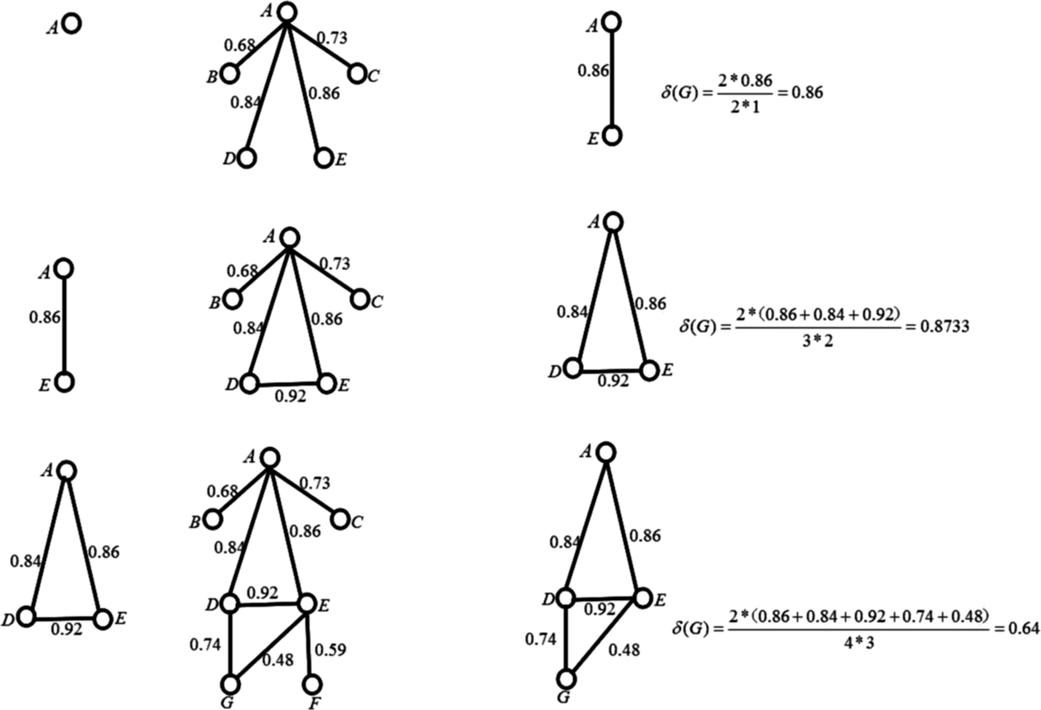
An example of the core's expansion process.

When the construction of core is complete, the next problem is how to determine the attachment. Equation (12) is considered as an evaluation function to measure the closeness between the attachment and the core, if the value of evaluation function is satisfactory enough, the protein represented by v in the function will be integrated into the core as an attachment. The complete process is described in Algorithm 5. \documentclass{aastex}\usepackage{amsbsy}\usepackage{amsfonts}\usepackage{amssymb}\usepackage{bm}\usepackage{mathrsfs}\usepackage{pifont}\usepackage{stmaryrd}\usepackage{textcomp}\usepackage{portland, xspace}\usepackage{amsmath, amsxtra}\usepackage{upgreek}\pagestyle{empty}\DeclareMathSizes{10}{9}{7}{6}\begin{document} \begin{align*} attachScore ( v , { V_ { subG } } ) = { \frac { \sum { _ { u \in { V_ { subG } } } { w_ { vu } } } } { \left\vert { { V_ { subG } } } \right\vert } } \tag { 12 } \end{align*} \end{document}

Algorithm 5: Candidate Protein Complexes
Input: core set, PN_j (PPI network at j time point)
Output: protein complexes with redundancy
1. complexes = { }
2. for core i in the core set:
3. new-complex = i
4. for each protein j in PN_j and j not in i:
5. if j is the adjacent of i:
6. Score = attachScore(j,core)
7. if Score>threshold:
8. j is chosen as an attachment
9. New-complex = i + j
10. end if
11. end if
12. complexes = complexes+New-complex
13. end for
14. end for

As shown in line 2, all of the cores are considered as a complex firstly, then line 4 considers the proteins in the PPI network who is the adjacent points of the proteins in the core but not in the core, will be the alternative attachments; if its attach-score is more than the threshold which is value of 0.3 in this article, the alternative attachment will be added into the complex, as performed in lines 4–13. At last, a full complexes set will be gotten. However, there is a lot of redundancy among the complexes, so we proposed another algorithm to eliminate the redundancy. Each protein complex can be regarded as a set, the method of handling sets is applied to compute the similarity between two different complexes as expressed in the Equation (13) (Lakizadeh et al., 2015): \documentclass{aastex}\usepackage{amsbsy}\usepackage{amsfonts}\usepackage{amssymb}\usepackage{bm}\usepackage{mathrsfs}\usepackage{pifont}\usepackage{stmaryrd}\usepackage{textcomp}\usepackage{portland, xspace}\usepackage{amsmath, amsxtra}\usepackage{upgreek}\pagestyle{empty}\DeclareMathSizes{10}{9}{7}{6}\begin{document} \begin{align*} sim ( { c_i } , { c_j } ) = { \frac { \left\vert { { c_i } \cap { c_j } } \right\vert } { \max ( \left\vert { { c_i } } \right\vert , \left\vert { { c_j } } \right\vert ) } } \tag { 13 } \end{align*} \end{document}

In Algorithm 6, there are three situations that need to be discussed. The first one is if there are two different size complexes with high similarity, the complex with smaller size will be regarded as a benchmark, and the protein in the set difference of the two complexes will be considered only if it can be added into the benchmark by the attachment score function. The second situation is if there are two same size complexes with high similarity in line 15, under this condition, the protein complex with high graph density will be selected, and the complex with lower graph density will be abandoned. The third situation is that if two complexes are not similar to each other, then both of the protein complexes will be chosen to expand the set of complex. The threshold in Algorithm 6 is equal to 0.7.

Algorithm 6: Eliminating Redundancy
Input: complexes1 from Algorithm 4
Output: complexes2 without redundancy
1. complexes2 = { }
2. for i in complexes1 do
3. for j in complexes1 do
4. if sim(i,j)<threshold1 then
5. C1 = min(size(i),size(j))
6. C2 = max(size(i),size(j))
7. Red-protein = C2-C1
8. if size(C2)! = size(C1) then
9. for k in red-protein do
10. if attachScore(k,C1)>threshold then
11. C1 = C1+k
12. complexes2 = complexes2+C1
13. end if
14. end for
15. else
16. density1 = \documentclass{aastex}\usepackage{amsbsy}\usepackage{amsfonts}\usepackage{amssymb}\usepackage{bm}\usepackage{mathrsfs}\usepackage{pifont}\usepackage{stmaryrd}\usepackage{textcomp}\usepackage{portland, xspace}\usepackage{amsmath, amsxtra}\usepackage{upgreek}\pagestyle{empty}\DeclareMathSizes{10}{9}{7}{6}\begin{document} $$\delta ( i )$$ \end{document}
17. density2 = \documentclass{aastex}\usepackage{amsbsy}\usepackage{amsfonts}\usepackage{amssymb}\usepackage{bm}\usepackage{mathrsfs}\usepackage{pifont}\usepackage{stmaryrd}\usepackage{textcomp}\usepackage{portland, xspace}\usepackage{amsmath, amsxtra}\usepackage{upgreek}\pagestyle{empty}\DeclareMathSizes{10}{9}{7}{6}\begin{document} $$\delta ( j )$$ \end{document}
18. den-pro = max(density1,density2)
19. complexes2 = complexes2+den-pro
20. end if
21. else
22. complexes2 = complexes2+i+j
23. end if
24. end for
25. end for
26. return complexes2

Algorithm 4: Subfunction: Core-Expand (Core, Subgraph)
Input: core, subgraph
Output: selected protein with max weight sum
1. for each protein l in core:
2. for each protein j in PN_j:
3. if j is the adjacent of l:
4. subgraph.add(j)
5. end for
6. end for
7. for p in subgraph and p not in core:
8. \documentclass{aastex}\usepackage{amsbsy}\usepackage{amsfonts}\usepackage{amssymb}\usepackage{bm}\usepackage{mathrsfs}\usepackage{pifont}\usepackage{stmaryrd}\usepackage{textcomp}\usepackage{portland, xspace}\usepackage{amsmath, amsxtra}\usepackage{upgreek}\pagestyle{empty}\DeclareMathSizes{10}{9}{7}{6}\begin{document} $$sub - {w_p} = \mathop \sum \limits_k {sub - {w_{pk}}}$$ \end{document}
9. end for
10. return max(sub-w_p)

Some highly active proteins express in most of time points, which leads to the fact that there will be a large part of repetition among the complexes predicted at different time points. So removing the redundant parts from the protein complexes composed of the smaller complexes is necessary. In Algorithm 6, eliminating redundancy algorithm will be applied again with all of the complexes predicted at each time point as the input.

To sum up, our method employs several extraordinary ideas which have not seen in other publications:

1. The PPI networks are shifted from static to dynamic; as the expression value of different proteins varies in different time points and various situations, not all of the protein interactions are active at all times, an improved three-sigma method is introduced to estimate the time when the interaction will be active. The improved three-sigma method with interval estimation shows better results in the sample's mean and variance.

2. Existing algorithms for predicting the protein complexes are inadequate for the PPI networks with weight. A new method that derives from the “core-attachment” structure will decrease the possibility of high overlap among the different protein complexes and improve the Acc of predicting results.

3. In the traditional approach, while calculating the weight of PPI network, only the topological structure information is considered. The biological information is not taken into computation of network's weight. Our approach first applied the GO annotation, implicit biological information, into computing the semantic similarity as the weight between two proteins. Besides, multiple methods integration has been used to calculate semantic similarity from different aspects.

3. Result and Evaluation Metrics

In this section, we first introduced several evaluation metrics. Then, we described the database including the protein interaction database, gene expression data, and the benchmark protein complex data used in our experiments. Last, we discussed the detail of experimental result, presented the effect of the parameters on the experiment. The result of our method proved that integrating expression data and GO semantic similarity with protein interaction data is an effective approach for predicting protein complexes.

3.1. Evaluation metrics

To evaluate our method and compare it with the benchmark, several evaluation metrics such as precision, recall, F-measure, and other respects are given in this section.

First, the neighborhood affinity score that is used to measure the match degree among the predicted complexes and the actual complexes is defined as follows: \documentclass{aastex}\usepackage{amsbsy}\usepackage{amsfonts}\usepackage{amssymb}\usepackage{bm}\usepackage{mathrsfs}\usepackage{pifont}\usepackage{stmaryrd}\usepackage{textcomp}\usepackage{portland, xspace}\usepackage{amsmath, amsxtra}\usepackage{upgreek}\pagestyle{empty}\DeclareMathSizes{10}{9}{7}{6}\begin{document} \begin{align*} NA ( P , B ) = { \frac { { { \left\vert { { V_P } \cap { V_B } } \right\vert } ^2 } } { \left\vert { { V_P } } \right\vert \times \left\vert { { V_B } } \right\vert } } , \end{align*} \end{document}

where P is a predicted complex, B is the benchmark complex, and V_i is the vertex set of i. Based on the experience from the previous article (Kouhsar et al., 2016), when \documentclass{aastex}\usepackage{amsbsy}\usepackage{amsfonts}\usepackage{amssymb}\usepackage{bm}\usepackage{mathrsfs}\usepackage{pifont}\usepackage{stmaryrd}\usepackage{textcomp}\usepackage{portland, xspace}\usepackage{amsmath, amsxtra}\usepackage{upgreek}\pagestyle{empty}\DeclareMathSizes{10}{9}{7}{6}\begin{document} $$NA ( p , b ) \ge { \rm{w}}$$ \end{document} and parameter w is usually 0.2, it is said the predicted complexes P match well with the benchmark B. If the predicted complex matches at least one complex in the benchmark, then the predicted complex will be appended to the set N_cp expressed as follows: \documentclass{aastex}\usepackage{amsbsy}\usepackage{amsfonts}\usepackage{amssymb}\usepackage{bm}\usepackage{mathrsfs}\usepackage{pifont}\usepackage{stmaryrd}\usepackage{textcomp}\usepackage{portland, xspace}\usepackage{amsmath, amsxtra}\usepackage{upgreek}\pagestyle{empty}\DeclareMathSizes{10}{9}{7}{6}\begin{document} \begin{align*} {N_{cp}} = \{ p \vert p \in P , \exists b \in B , NA ( p , b ) \ge 0.2 \} . \end{align*} \end{document}

The same argument applies to the set N_cb: \documentclass{aastex}\usepackage{amsbsy}\usepackage{amsfonts}\usepackage{amssymb}\usepackage{bm}\usepackage{mathrsfs}\usepackage{pifont}\usepackage{stmaryrd}\usepackage{textcomp}\usepackage{portland, xspace}\usepackage{amsmath, amsxtra}\usepackage{upgreek}\pagestyle{empty}\DeclareMathSizes{10}{9}{7}{6}\begin{document} \begin{align*} {N_{cb}} = \{ b \vert b \in B , \exists p \in P , NA ( p , b ) \ge 0.2 \} , \end{align*} \end{document}

in which the benchmark complex must match at least one complex predicted by out method. Based on the definition of neighborhood affinity score, the metrics including precision, recall, and F-measure can be expressed as follows: \documentclass{aastex}\usepackage{amsbsy}\usepackage{amsfonts}\usepackage{amssymb}\usepackage{bm}\usepackage{mathrsfs}\usepackage{pifont}\usepackage{stmaryrd}\usepackage{textcomp}\usepackage{portland, xspace}\usepackage{amsmath, amsxtra}\usepackage{upgreek}\pagestyle{empty}\DeclareMathSizes{10}{9}{7}{6}\begin{document} \begin{align*} precision = { \frac { \left\vert { { N_ { cp } } } \right\vert } { \left\vert P \right\vert } } . \end{align*} \end{document} \documentclass{aastex}\usepackage{amsbsy}\usepackage{amsfonts}\usepackage{amssymb}\usepackage{bm}\usepackage{mathrsfs}\usepackage{pifont}\usepackage{stmaryrd}\usepackage{textcomp}\usepackage{portland, xspace}\usepackage{amsmath, amsxtra}\usepackage{upgreek}\pagestyle{empty}\DeclareMathSizes{10}{9}{7}{6}\begin{document} \begin{align*} recall = { \frac { \left\vert { { N_ { cb } } } \right\vert } { \left\vert b \right\vert } } . \end{align*} \end{document} \documentclass{aastex}\usepackage{amsbsy}\usepackage{amsfonts}\usepackage{amssymb}\usepackage{bm}\usepackage{mathrsfs}\usepackage{pifont}\usepackage{stmaryrd}\usepackage{textcomp}\usepackage{portland, xspace}\usepackage{amsmath, amsxtra}\usepackage{upgreek}\pagestyle{empty}\DeclareMathSizes{10}{9}{7}{6}\begin{document} \begin{align*} F = { \frac { { \rm { 2 } } \times precision \times recall } { precision + recall } } . \end{align*} \end{document}

The precision value describes how many protein complexes predicted by a method are correct. In contrast, what the recall expresses is that how many benchmark complexes or known complexes have been indexed by the method. Sometimes the precision and the recall have an impact on each other, so F-measure is introduced to balance precision and recall. In addition to that, sensitivity (Sn), positive predictive value (PPV), and Acc are another group of evaluation metrics introduced in this article. If we denote \documentclass{aastex}\usepackage{amsbsy}\usepackage{amsfonts}\usepackage{amssymb}\usepackage{bm}\usepackage{mathrsfs}\usepackage{pifont}\usepackage{stmaryrd}\usepackage{textcomp}\usepackage{portland, xspace}\usepackage{amsmath, amsxtra}\usepackage{upgreek}\pagestyle{empty}\DeclareMathSizes{10}{9}{7}{6}\begin{document} $$m = \left\vert {{V_p}} \right\vert$$ \end{document} and \documentclass{aastex}\usepackage{amsbsy}\usepackage{amsfonts}\usepackage{amssymb}\usepackage{bm}\usepackage{mathrsfs}\usepackage{pifont}\usepackage{stmaryrd}\usepackage{textcomp}\usepackage{portland, xspace}\usepackage{amsmath, amsxtra}\usepackage{upgreek}\pagestyle{empty}\DeclareMathSizes{10}{9}{7}{6}\begin{document} $$n = \left\vert {{V_b}} \right\vert$$ \end{document} as the number of proteins in predicted complex and benchmark complex, respectively, \documentclass{aastex}\usepackage{amsbsy}\usepackage{amsfonts}\usepackage{amssymb}\usepackage{bm}\usepackage{mathrsfs}\usepackage{pifont}\usepackage{stmaryrd}\usepackage{textcomp}\usepackage{portland, xspace}\usepackage{amsmath, amsxtra}\usepackage{upgreek}\pagestyle{empty}\DeclareMathSizes{10}{9}{7}{6}\begin{document} $${T_{ij}}$$ \end{document} is the number of common proteins between the benchmark complex i and the predicted complex j. So the definition of Sn and PPV can be written as follows: \documentclass{aastex}\usepackage{amsbsy}\usepackage{amsfonts}\usepackage{amssymb}\usepackage{bm}\usepackage{mathrsfs}\usepackage{pifont}\usepackage{stmaryrd}\usepackage{textcomp}\usepackage{portland, xspace}\usepackage{amsmath, amsxtra}\usepackage{upgreek}\pagestyle{empty}\DeclareMathSizes{10}{9}{7}{6}\begin{document} \begin{align*} Sn = { \frac { \mathop \sum \limits_ { i = 1 } ^n { \mathop { \max } \limits_j \ { { T_ { ij } } \ } } } { \mathop \sum \limits_ { i = 1 } ^n { { N_i } } } } , \end{align*} \end{document} \documentclass{aastex}\usepackage{amsbsy}\usepackage{amsfonts}\usepackage{amssymb}\usepackage{bm}\usepackage{mathrsfs}\usepackage{pifont}\usepackage{stmaryrd}\usepackage{textcomp}\usepackage{portland, xspace}\usepackage{amsmath, amsxtra}\usepackage{upgreek}\pagestyle{empty}\DeclareMathSizes{10}{9}{7}{6}\begin{document} \begin{align*} PPV = { \frac { \mathop \sum \limits_ { j = 1 } ^m { \mathop { \max } \limits_i \ { { T_ { ij } } \ } } } { \mathop \sum \limits_ { j = 1 } ^m { { T_ { .j } } } } } , \end{align*} \end{document}

where N_i is the number of proteins in the benchmark complex. There is another metric called Acc that is a combination of Sn and PPV. \documentclass{aastex}\usepackage{amsbsy}\usepackage{amsfonts}\usepackage{amssymb}\usepackage{bm}\usepackage{mathrsfs}\usepackage{pifont}\usepackage{stmaryrd}\usepackage{textcomp}\usepackage{portland, xspace}\usepackage{amsmath, amsxtra}\usepackage{upgreek}\pagestyle{empty}\DeclareMathSizes{10}{9}{7}{6}\begin{document} \begin{align*} Acc = \sqrt {Sn \times PPV}. \end{align*} \end{document}

Second, as another evaluation metric, Jaccard score is also introduced in this article to describe the matching degree, the range of Jaccard score is from 0 to 1. When the score is equal to 1, it means the predicted complexes match with the benchmark complexes exactly. Otherwise, if the score is equal to 0, it indicates that there is no intersection between the predicted complex and the benchmark complex.

3.2. Experiment database

In this article, the STRING data (Franceschini et al., 2013) are chosen as the PPI network data. In addition to the biological experimental data, data mining from the context abstract and other databases, there is also some PPI data predicted by bioinformatics method. GSE3431 (Tu and Mcknight, 2005) is introduced as the gene expression data. GO annotation file is downloaded from Saccharomyces Genome Database (Issel-Tarver et al., 2002). For the benchmark, we choose CYC2008 (Pu et al., 2009), which is composed of 408 protein complexes.

3.3. Experiment result analysis

In this part, we try to illustrate how our method is compared with other predictors through several comparative experiments.

3.3.1. The discussion of parameters in our method

From Table 1, first, we can seen that as the step increases, the number of active proteins drops slowly; second, although under the same step, there is also a large difference among the number of proteins at different time points, and the expression ability of a protein is the weakest at time point 12. Third, through the analysis of the table, it can be concluded that not all of the proteins are active all the time, their expression values change with time.

Table 1.

The Effect of Different Steps on the Number of Active Proteins at Each Time Point

	Time = 1	Time = 2	Time = 3	Time = 4	Time = 5	Time = 6	Time = 7	Time = 8	Time = 9	Time = 10	Time = 11	Time = 12
Step = 0	4071	4100	3706	3606	3676	3339	3399	3035	3836	3262	3409	2991
Step = 1	3464	3502	3123	3007	3086	2754	2757	2665	3426	2699	2840	2423
Step = 2	2982	3016	2708	2542	2636	2302	2308	2378	2947	2258	2398	1969
Step = 3	2571	2608	2344	2167	2285	1947	1964	2130	2544	1904	2030	1614
Step = 4	2213	2270	2024	1827	1971	1614	1671	1878	2229	1611	1729	1317
Step = 5	1910	1970	1746	1553	1693	1362	1394	1642	1971	1356	1456	1109
Step = 6	1637	1725	1528	1294	1446	1129	1180	1440	1727	1130	1217	930
Step = 7	1406	1500	1281	1094	1234	936	989	1260	1513	967	1015	754
Step = 8	1229	1302	1103	927	1049	774	833	1089	1323	804	854	603
Step = 9	1058	1134	952	788	892	633	693	940	1151	683	694	477
Step = 10	927	991	798	629	734	531	579	812	1018	554	574	391
Step = 11	787	859	664	517	606	424	483	709	892	462	463	312
Step = 12	681	736	561	401	510	345	394	622	762	374	386	241

Bold/italic values are the maximum or minimum in each row.

Table 2 is to find the most appropriate parameter d in the improved three-sigma method; it illustrates the impact of different steps on the experimental results under the same threshold conditions. It is evident that the highest value of precision and PPV are 0.536 and 0.347, respectively, when the step parameter is 9; in addition, the comprehensive indicators F-measure and Acc that arrive at the peak point are 0.438 and 0.374, respectively, when the step parameter is 10, which means that both of the mean and variance adopted in the three-sigma method are better than sample mean and variance. From Table 2, it can be concluded that our method can perform better at the condition that the step parameter is equal to 10.

Table 2.

The Effect of Steps on the Evaluation Metrics (Complex-Threshold = 0.2)

	Precision	Recall	F-measure	Sn	PPV	Acc
Step = 1	0.352	0.380	0.366	0.350	0.204	0.267
Step = 2	0.298	0.222	0.255	0.211	0.245	0.227
Step = 3	0.329	0.178	0.231	0.162	0.246	0.200
Step = 4	0.360	0.172	0.232	0.201	0.252	0.225
Step = 5	0.388	0.134	0.199	0.170	0.258	0.209
Step = 6	0.442	0.061	0.108	0.058	0.277	0.127
Step = 7	0.405	0.045	0.081	0.037	0.301	0.105
Step = 8	0.405	0.031	0.058	0.027	0.320	0.093
Step = 9	0.536	0.018	0.034	0.012	0.347	0.065
Step = 10	0.328	0.665	0.438	0.711	0.197	0.374
Step = 11	0.328	0.654	0.437	0.709	0.197	0.373
Step = 12	0.328	0.655	0.437	0.709	0.191	0.368

Acc, accuracy; PPV, positive predictive value; Sn, sensitivity.

Bold/italic values are the maximum in each column.

In Algorithm 2—seed-Generate, the cluster-threshold representing the density of a seed set is set to control the seed size, if the lower the cluster-threshold is, the larger the size of seed will be. So the result of predicted protein complexes is closely related to the cluster-threshold value. To determine the optimal cluster-threshold parameter, as shown in Table 3, we compare the experiment results produced under different parameters. As illustrated in Table 3, when cluster-threshold is 0.2, our method performs best on predicting protein complexes. In contrast, it also reflects another drawback of our method that the experimental results depend on the number and value of parameters.

Table 3.

The Effect of Cluster-Threshold on the Evaluation Metrics (Step = 10)

Threshold	Precision	Recall	F-measure	Sn	PPV	Acc
0.1	0.257	0.504	0.341	0.695	0.179	0.352
0.2	0.382	0.665	0.486	0.640	0.156	0.356
0.3	0.295	0.617	0.399	0.698	0.182	0.357
0.4	0.302	0.631	0.409	0.708	0.195	0.372
0.5	0.324	0.650	0.433	0.708	0.196	0.373
0.6	0.330	0.653	0.438	0.701	0.187	0.362
0.7	0.313	0.634	0.419	0.711	0.197	0.374
0.8	0.140	0.110	0.123	0.795	0.098	0.279
0.9	0.245	0.020	0.038	0.276	0.079	0.148

Bold/italic values are the maximum in each column.

If we check the time point wherein all of the three evaluation metrics, precision, recall, and F-measure, reach their maximum point, we have found that they achieve the highest value of 0.382, 0.665, and 0.486, respectively. However, Sn arrives at the highest value with 0.795 when cluster-threshold is 0.8, and PPV and Acc come to the best value with 0.197 and 0.374 when cluster-threshold is 0.7. From Table 3, it can be found that when the cluster-threshold is >0.7, the values of precision and recall decrease. It is related to the PPI data used in the experiment, because the weighted density of most subnetworks constructed in this article is <0.8, resulting in few seeds chosen.

The attachment score threshold is introduced in Algorithm 5 to detect protein complex. To find the appropriate threshold, our method is run on the dynamic PPI network. As shown in Figure 8, the values of Acc remain stable under various thresholds, but the values of F-measure fluctuate slightly. Among the range from 0.15 to 0.7, it keeps stable and averages at 0.43; however, when the threshold is >0.75, the values of F-measure decrease to around 0.4. According to this experiment, attachment score threshold is set to 0.6 as default.

FIG. 8.

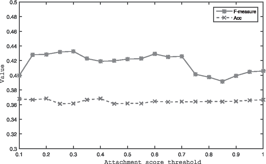
The F-measure and Acc values of our method for various values of attachment score threshold. Acc, accuracy.

3.3.2. Semantic similarity score analysis

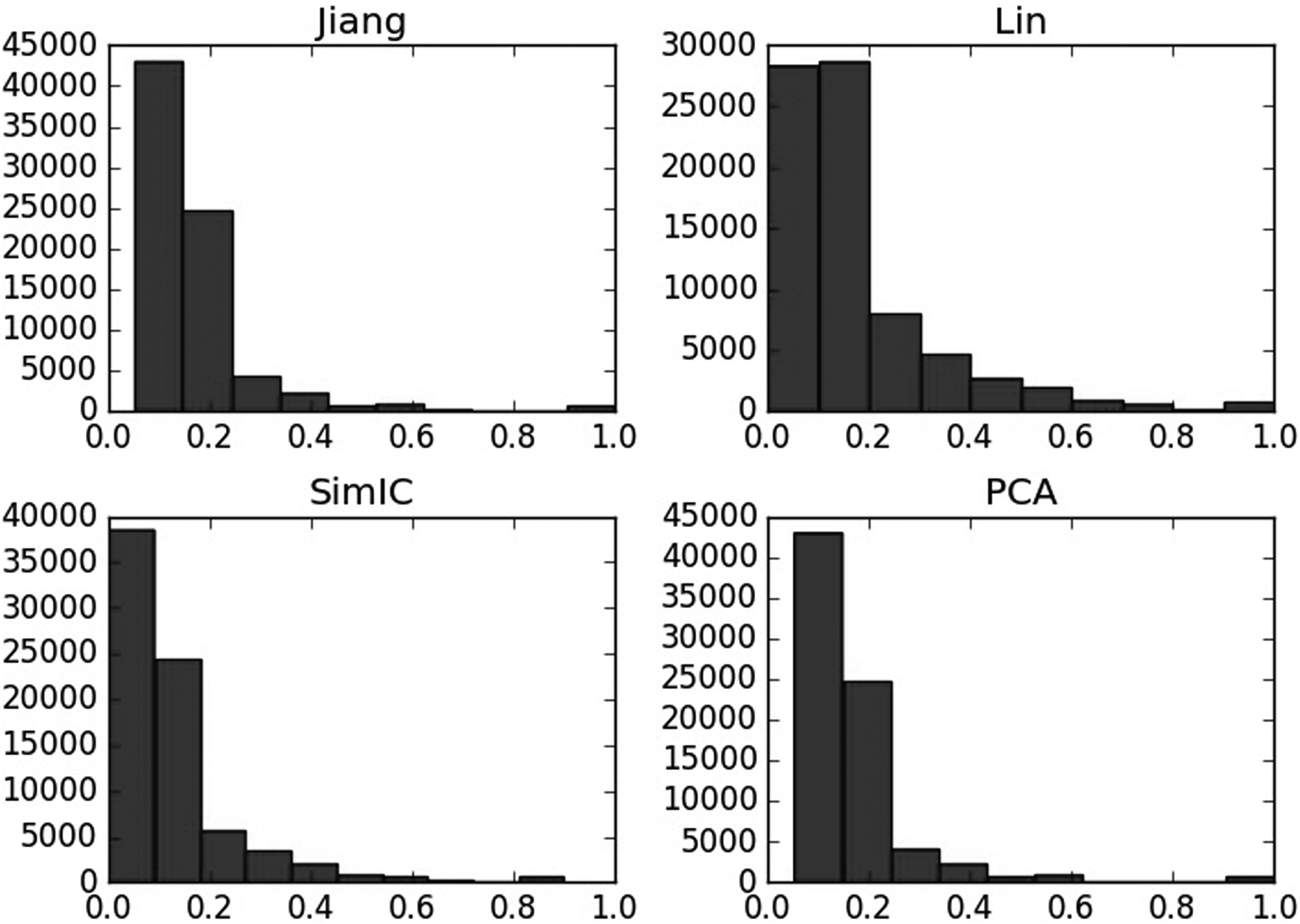
To analyze the semantic similarity computed by different methods, frequency statistical graphs in these three aspects including BP, CC, and MF are introduced. As shown in Figures 9 –11, even though in the same aspects, the semantic similarity scores vary greatly according to the computational methods. For example, Figure 9 describes that when computing the semantic similarity in BP, the scores of Jiang's method are mainly distributed from 0.1 to 0.2; the range of Lin's method covers from 0 to 0.8, which is much wider than Jiang's and SimIC's; also, the score frequency of SimIC's method decreases gradually, most of the scores distribute between 0 and 0.3. However, most of scores measured by PCA are still between 0 and 0.2, and the range of similarity is also as wide as the Lin's method, so PCA integrates the advantages of the other three measures.

FIG. 9.

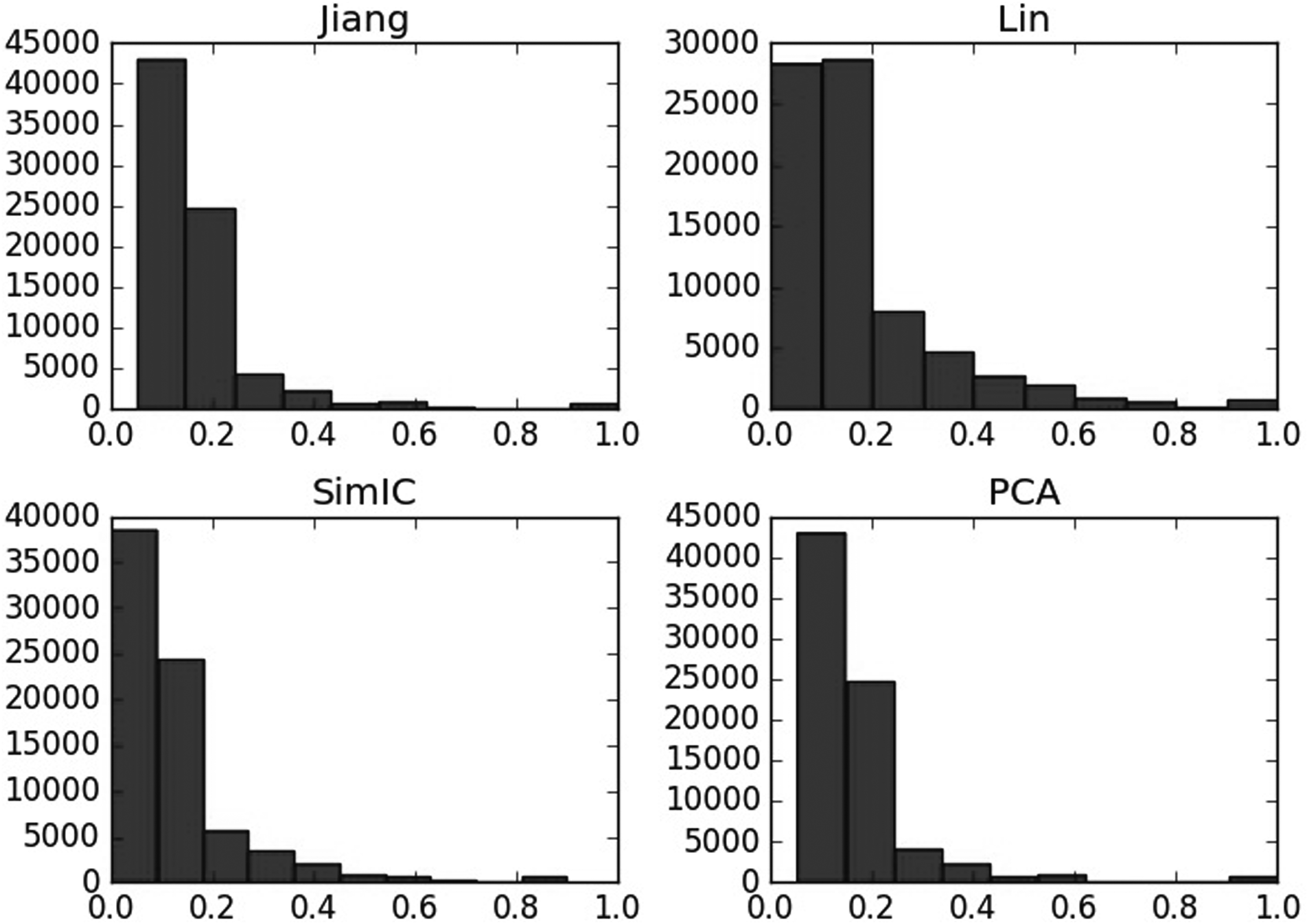
Semantic similarity frequency statistical graph of different methods on biological process. PCA, principal component analysis.

FIG. 10.

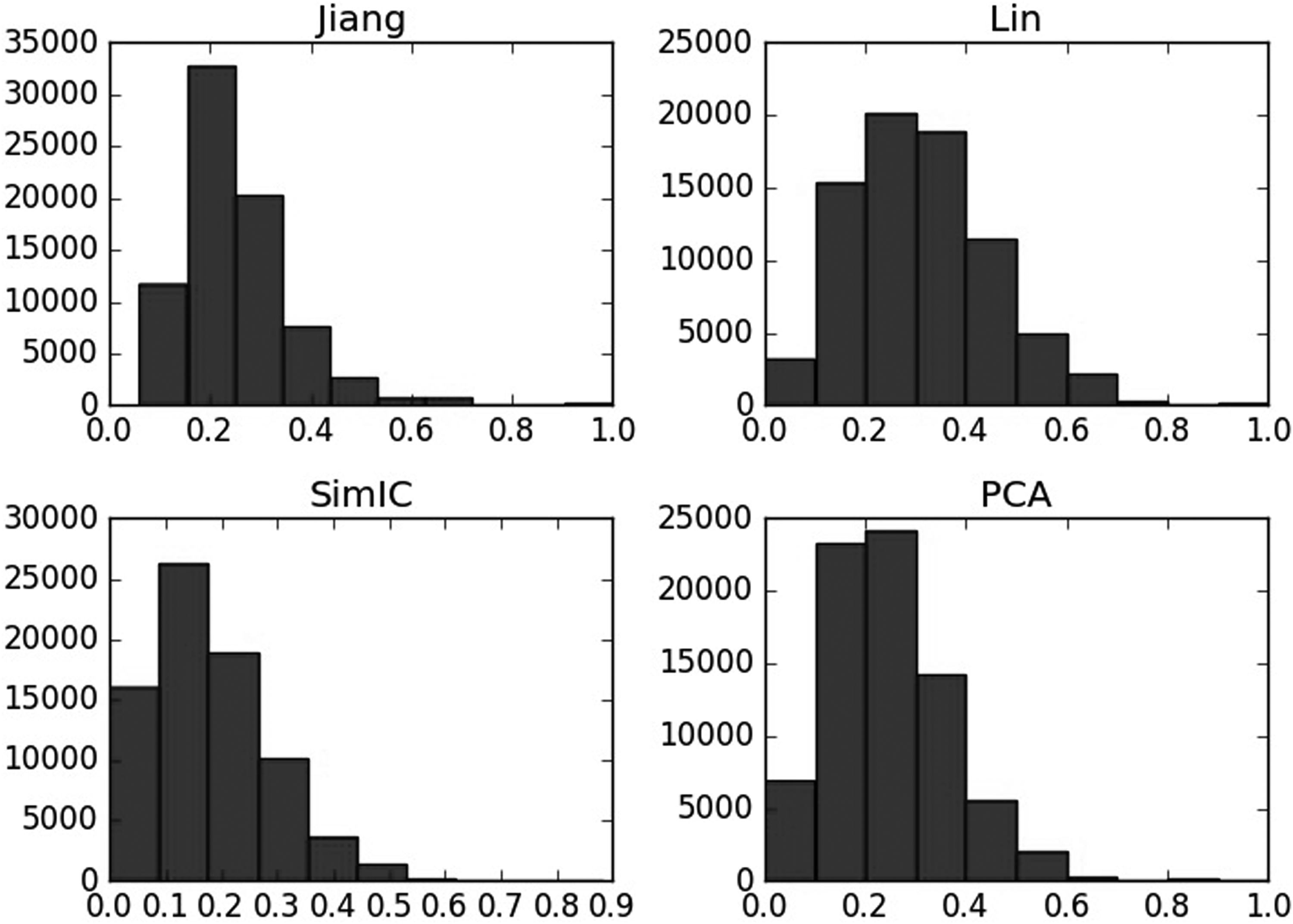
Semantic similarity frequency statistical graph of different methods on cellular component.

FIG. 11.

Semantic similarity frequency statistical graph of different methods on molecular function.

In addition, Figure 12 shows the effect of different semantic similarity methods on the experimental results. It is clear that the precision, recall, and F-measure of the weighted networks that have been processed by PCA perform better than the other three methods. Furthermore, the icon also confirms that the PCA plays a positive role in removing data noise and improving the Acc of prediction results.

FIG. 12.

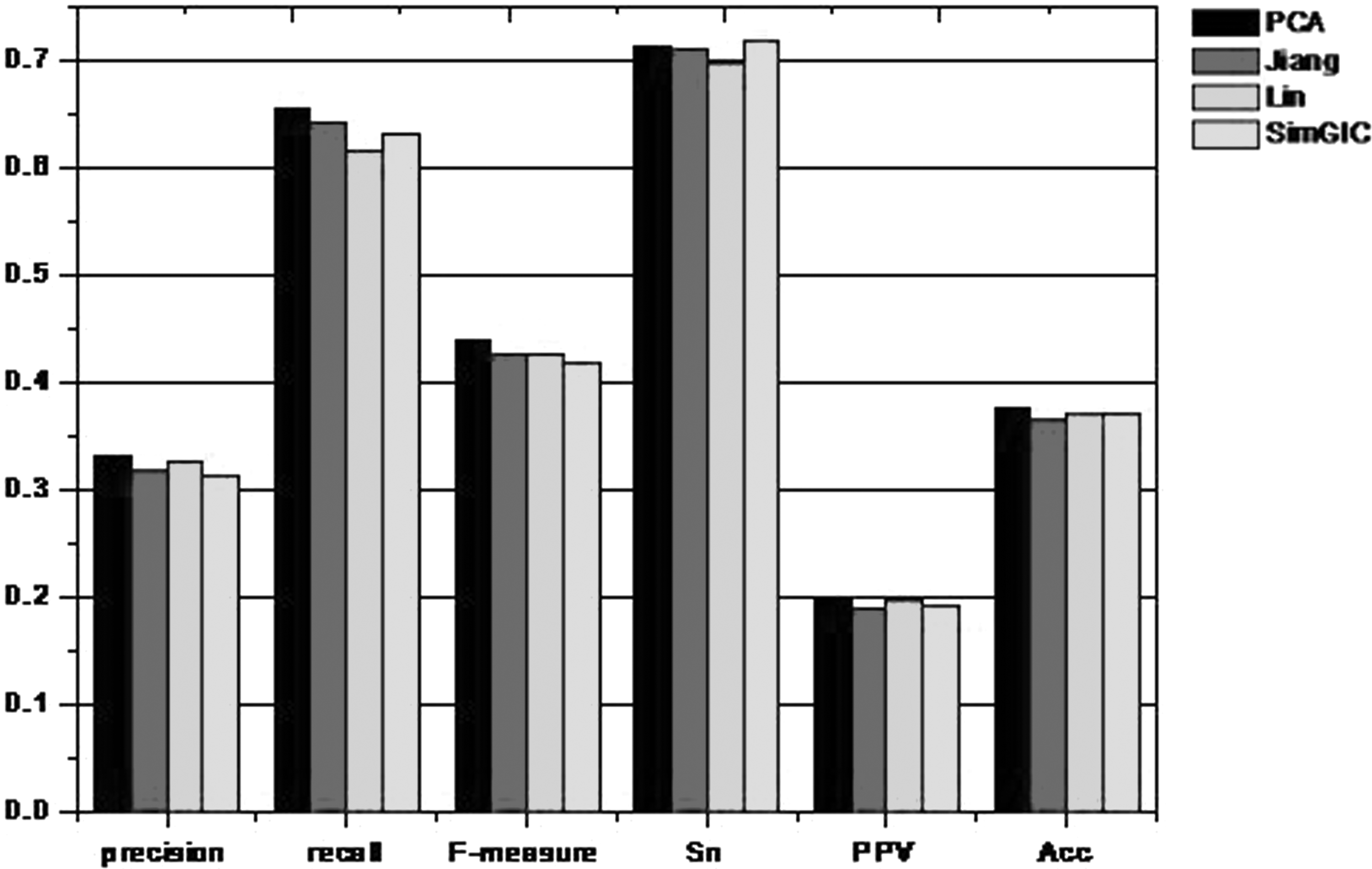
Results compared with different semantic similarity.

3.3.3. Comparison with the known complex

Figure 13 shows the change of Jaccard score from our method at each time point, it reaches a peak of 0.38 with the bottom around 0.27, and from the figure it can also be concluded that the Jaccard scores fluctuate significantly, so the average value is chosen as the evaluating indicator finally to compare with other methods. Besides, the unstable Jaccard values also reveal the dynamics of the PPI network built in this article.

FIG. 13.

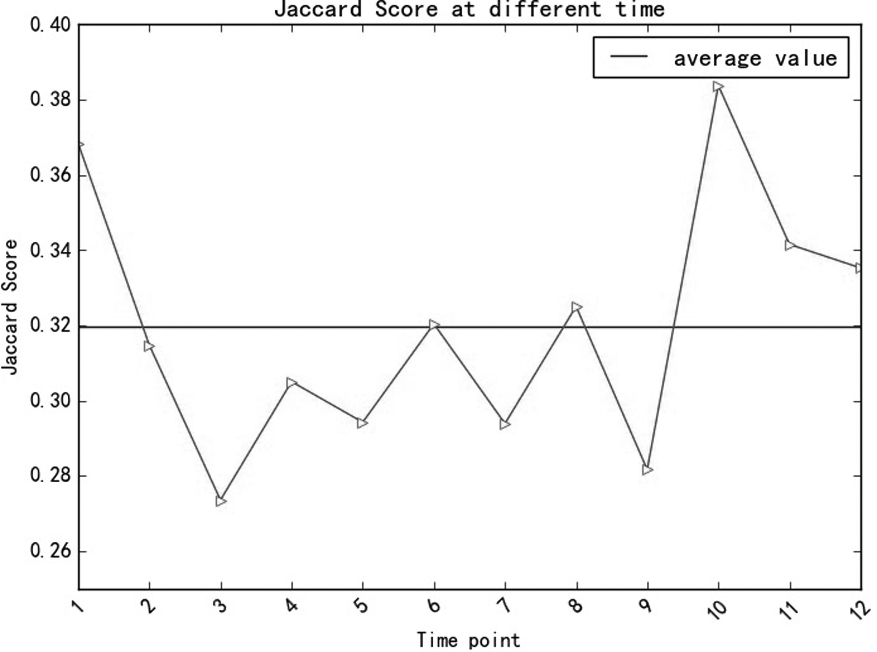
Jaccard scores of our method at different time points.

We compared our method with other classical algorithms, such as the coach (Lakizadeh et al., 2015), WCOACH (Price et al., 2013), MCODE (Bader and Hogue, 2003), MCODE-weight (Price et al., 2013), and Ipca (Min et al., 2008) to assess the predictor carefully. And as shown in Table 4, all of the Jaccard scores are around 0.3, the score predicted by the MCODE method is the lowest with 0.2913. In contrast, our method performs slightly better than WCOACH and MCODE-weight method, 0.31975, 0.30572, and 0.30285, respectively. So the table confirms that our method may perform well in predicting protein complexes.

Table 4.

The Comparison of the Jaccard Score of Six Methods

Method	WCOACH	Coach	MCODE-weight	MCODE	Ipca	Our method
Jaccard score	0.30572	0.29677	0.30285	0.29130	0.29522	0.31975

To be objective, all algorithms are run in the same PPI data and the same benchmark is selected. Figure 14 shows the corresponding precision–recall graphs comparing different traditional cluster algorithms with our method proposed in this article. In most of the recall range, our method still maintains greater precision, in addition, our method outperforms with significantly higher recall, as well as greater precision among the initial top predictions (at recall <0.4).

FIG. 14.

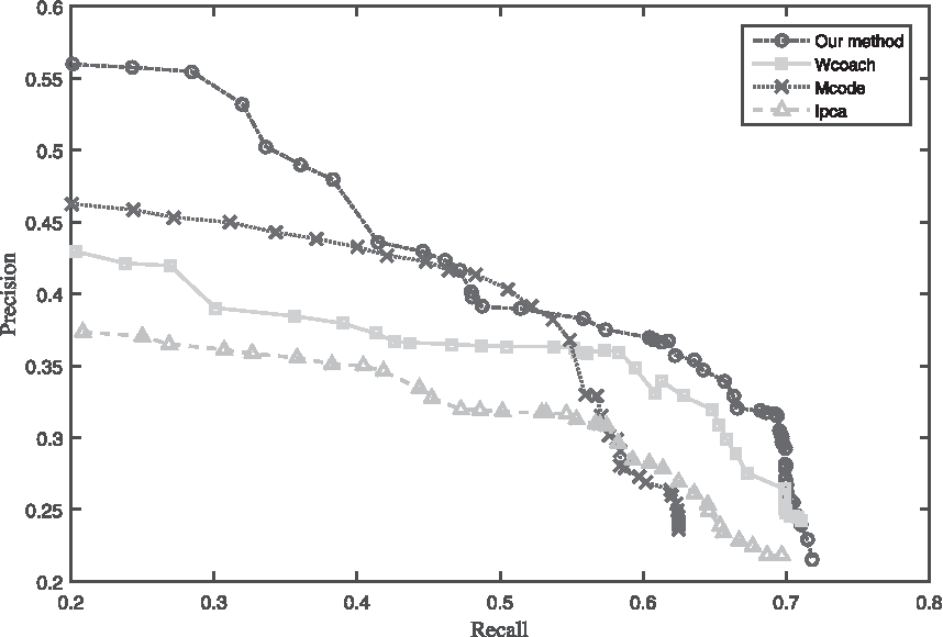
Precision–recall graph of four cluster algorithms.

It is clearly observed from Figure 15 that our method proposed in this article reaches the highest precision, recall, and F-measure. The Sn value of coach algorithm is higher, but its PPV reduces to 0.14, which leads to a worse Acc value. Both our method and coach algorithm are in light of “core-attachment,” but some details such as density formula, eliminating redundancy, are different. Nevertheless, precision, recall, and F-measure of our method perform better, which illustrates that our method improves the Acc of predicting protein complexes. Moreover, our method introduced semantic similarity dealt with PCA as the weight between PPIs. Although the other two classical algorithms, WCOACH and MCODE-weight, are introduced to predict protein complexes from weighted PPI networks, unfortunately, these two algorithms' effect is not as good as our method, their precision, recall, and F-measure are less than our method. It indicates that semantic similarity dealt with PCA works better than other approaches. In summary, it is assumed that our method effectively improves the prediction Acc of protein complexes.

FIG. 15.

Results compared with different algorithm.

4. Conclusions

This article proposed an approach to integrate multiple techniques to improve the predicting Acc of the protein complexes. First, we integrate static PPI networks with gene expression data to construct a dynamic network through combining interval estimation with the three-sigma method. The improved method performs better on the data set with low expression values than the original method. Secondly, GO semantic similarity that contains biological information is applied to filter redundant information and process the weight of network. It proves that GO semantic similarity reflects the degree of intimacy between the two proteins better than the topological information. Third, after building a weighted PPI dynamic network, DWCOACH is introduced to predict protein complexes. And, it decreases the overlap among different protein complexes and improves the prediction Acc. Several experiments are conducted and the results prove that our algorithm performs better than other algorithms on selected evaluation metrics. We also observed that there are some drawbacks in our method, for example, the test result is sensitive to the number and value of parameters, which indicates that more experiments should be carried out to find out the best parameter values.

Footnotes

Acknowledgments

This work was supported, in part, by National Science Foundation of China under Grant No. 61402304, the Humanity and Social Science general project of Ministry of Education under Grant No.14YJAZH046, the Beijing Natural Science Foundation under Grant No. 4154065, the Beijing Educational Committee Science and Technology Development Planned under Grant No. KM201610028015, Science and Technology Innovation Platform, Teaching Teacher, and Connotation Development of Colleges and Universities.

Author Disclosure Statement

No competing financial interests exist.

References

Bader

G.D.

, and Hogue

C.W.

2003. An automated method for finding molecular complexes in large protein interaction networks. BMC Bioinf. 4, 2–14.

Chen

, Fan

, Liu

, et al. 2014. Identifying protein complexes and functional modules from static PPI networks to dynamic PPI networks. Brief. Bioinform., 15, 177–194.

Dezso

, Oltvai

Z.N.

, and Barabási

A.L.

2003. Bioinformatics analysis of experimentally determined protein complexes in the yeast Saccharomyces cerevisiae. Genome Res. 13, 2450–2466.

Franceschini

, Szklarczyk

, Frankild

, et al. 2013. STRING v9.1: protein–protein interaction networks, with increased coverage and integration. Nucleic Acids Res. 41, D808–D815.

Gavin

A.-C.

, Aloy

, Grandi

, et al. 2006. Proteome survey reveals modularity of the yeast cell machinery. Nature. 440, 631–636.

Girvan

, and Newman

M.E.J.

2001. Community structure in social and biological networks. PNAS. 99, 7821–7826.

Hayashida

, Kamada

, Song

, et al. 2011. Conditional random field approach to prediction of protein–protein interactions using domain information. BMC Syst. Biol., 5, 1–9.

Issel-Tarver

, Christie

K.R.

, Dolinski

, et al. 2002. Saccharomyces genome database. Methods Enzymol. 350, 329–335.

Jiang

J.J.

, and Conrath

D.W.

1997. Semantic similarity based on corpus statistics and lexical taxonomy. Presented in Proceedings of International Conference Research on Computational Linguistics (ROCLING X), Taiwan.

10.

King

A.D.

, Pržulj

, and Jurisica

2012. Protein complex prediction with RNSC. Methods Mol. Biol., 804, 297–312.

11.

Kouhsar

, Zaremirakabad

, and Jamali

2016. MWCOACH: Protein complex prediction in weighted PPI networks. Genes Genet Syst. 91, 317–324.

12.

Lakizadeh

, Jalili

, and Marashi . 2015. PCD-GED: Protein complex detection considering PPI dynamics based on time series gene expression data. J. Theor. Biol., 378, 31–38.

13.

, Li

, Wang

, et al. 2012. Algorithm for identification of protein complexes using topological information of PPI network. J. Inf. Comput. Sci. 9, 3459–3467.

14.

Lin

1998. An information-theoretic definition of similarity. Presented in 15th International Conference on Machine Learning, San Francisco.

15.

Liu

, Wong

, and Chua

H.N.

2009. Complex discovery from weighted PPI networks. Bioinformatics. 25, 1891–1897.

16.

, Cho

Y.R.

, and Chiam

T.C.

2012. M-finder: Functional association mining from protein interaction networks weighted by semantic similarity. IEEE International Conference on Bioinformatics and Biomedicine, Washington.

17.

, Mcanulla

, and Wang

2012. Protein complex prediction based on maximum matching with domain domain interaction. BBA. 1824, 1418–1424.

18.

Min

, Chen

J.E.

, Wang

J.X.

, et al. 2008. Modifying the dpclus algorithm for identifying protein complexes based on new topological structures. BMC Bioinf. 9, 1–16.

19.

Ozawa

, Saito

, Fujimori

, et al. 2010. Protein complex prediction via verifying and reconstructing the topology of domain–domain interactions. BMC Bioinf. 11, 1–12.

20.

Palla

, Dernyi

, and Vicsek

2007. The critical point of k-clique percolation in the Erdős–Rényi graph. J. Stat. Phys., 128, 219–227.

21.

Price

, Rd

P.F.

, and Cho

Y.R.

2013. Survey: Enhancing protein complex prediction in PPI networks with go similarity weighting. Interdiscip. Sci., 5, 196–210.

22.

, Wong

, Turner

, et al. 2009. Up-to-date catalogues of yeast protein complexes. Nucleic Acids Res. 37, 825–831.

23.

Shigehiko

, Ken

, Kenji

, et al. 2006. Development and implementation of an algorithm for detection of protein complexes in large interaction networks. BMC Bioinf. 7, 1–13.

24.

Shih

Y.K.

, and Parthasarathy

2012. Identifying functional modules in interaction networks through overlapping markov clustering. Bioinformatics. 28, i473–i479.

25.

Spirin

A.S.

2004. High-throughput cell-free systems for synthesis of functionally active proteins. Trends Biotechnol. 22, 538–545.

26.

Srihari

, Ning

, and Leong

H.W.

2010. MCL-caw: A re-nement of MCL for detecting yeast complexes from weighted PPI networks by incorporating core-attachment structure. BMC Bioinf. 11, 504–528.

27.

B.P.

, and Mcknight

S.L.

2005. Logic of the yeast metabolic cycle: Temporal compartmentalization of cellular processes. Science. 310, 1152–1158.

28.

Wang

, Peng

, Li

, et al. 2013. Construction and application of dynamic protein interaction network based on time course gene expression data. Proteomics. 13, 301–312.

29.

Wang

, Xie

, Lin

, et al. 2011. Identifying protein complexes from PPI networks using go semantic similarity. Presented in IEEE International Conference on Bioinformatics and Biomedicine, Washington.

A Method for Predicting Protein Complexes from Dynamic Weighted Protein–Protein Interaction Networks

Abstract

Abstract

1. Introduction

2. Methods

2.1. Determine the interval of population's mean and variance

2.2. Improved three-sigma method

2.3. GO semantic similarity

2.4. Algorithm of predicting protein complexes

3. Result and Evaluation Metrics

3.1. Evaluation metrics

3.2. Experiment database

3.3. Experiment result analysis

3.3.1. The discussion of parameters in our method

3.3.2. Semantic similarity score analysis

3.3.3. Comparison with the known complex

4. Conclusions

Footnotes

Acknowledgments

Author Disclosure Statement

References