Real-time genome comparison is important for identifying unknown species and clustering organisms. We propose a novel method that can represent genome sequences of different lengths as a 12-dimensional numerical vector in real time for this purpose. Given a genome sequence, a binary indicator sequence of each nucleotide base location is computed, and then discrete wavelet transform is applied to these four binary indicator sequences to attain the respective power spectra. Afterward, moments of the power spectra are calculated. Consequently, the 12-dimensional numerical vectors are constructed from the first three order moments. Our experimental results on various data sets show that the proposed method is efficient and effective to cluster genes and genomes. It runs significantly faster than other alignment-free and alignment-based methods.
1. Introduction
To identify newly emerging virus and bacteria threat (Malone et al., 2016) and also handle large genome data, it is necessary to develop a reliable real-time genome sequence clustering method. Using distance-based tree methods, the main challenge of real-time clustering is to transform genome sequences into numerical vectors. In addition, phylogenetic trees are helpful for scientists to understand the relationships of the organisms studied. In the past few decades, several alignment-based methods have been developed (Katoh et al., 2002; Edgar, 2004; Larkin et al., 2007). Although they provide accurate genome comparison results, they also require a lot of running time and memory consumption so that they may not be suitable for the need of quick clustering, especially for investigating emerging epidemic virus (Marra et al., 2003).
As a result, alignment-free techniques provide alternative choices that generally run fast (Vinga and Almeida, 2003; Yau et al., 2008; Yu et a., 2011, 2013; Huang et al., 2014; Huang, 2016; Huang and Yu, 2016). For example, the k-mer method is among the most popular alignment-free methods (Blaisdell, 1986; 1989; Comin and Verzotto, 2012; Vinga and Almeida, 2003; Pandit and Sinha, 2010). Recently, discrete Fourier transform (DFT) has gained popular interest in genome sequence clustering (Tiwari et al., 1997; Anastassiou, 2000; Kotlar and Lavner, 2003; Machado et al., 2011). A DFT power spectrum of a DNA sequence reflects the distribution of nucleotide base location, and it has been applied to identify protein coding regions, genes, and whole genome sequences (Yin and Yau, 2005, 2007; Hoang et al., 2015). Hoang et al. (2015) proposed an alignment-free method called power spectrum moments (PS-M) method. They tested PS-M on five different types of gene and genome sequence data sets and obtained satisfactory results in terms of clustering correctness and computational time.
Wu et al. (2000) compared DFT and discrete wavelet transform (DWT) and found that DWT runs faster than DFT with comparable time series similarity search in time series. In addition, DWT is able to capture both frequency and location information, whereas DFT cannot provide temporal resolution (Koo et al., 2011). Consequently, we propose an alignment-free clustering method that transforms genome sequences using DWT and clusters the resulting vectors by a distance-based tree.
2. Methods
2.1. Mathematical background
In signal processing, sequences in time domain are commonly transformed into frequency domain to make some important features visible. The DFT (Almeida, 1994) is a common method widely used in signal processing. A method using DFT and natural vector has been proposed for phylogenetic analysis (Hoang et al., 2015). This method uses the first three moments of the DFT of each nucleotide's binary position vector. The transformation of DFT has a global basis for the whole nucleotide sequence, so that it is less effective to preserve local variation. Unlike DFT, the DWT provides multiple resolutions to preserve local details and filter out noise. Hence we propose to use DWT to improve the numerical representation of genome sequences.
The DFT is often used to find the frequency components of a signal buried in a noisy time domain. Signal processing techniques primarily focus on analyzing features of a signal either in the time domain, frequency domain, or both. Transforms such as Fourier transforms are commonplace in visualizing a signal in frequency domain. For example, consider a signal \documentclass{aastex}\usepackage{amsbsy}\usepackage{amsfonts}\usepackage{amssymb}\usepackage{bm}\usepackage{mathrsfs}\usepackage{pifont}\usepackage{stmaryrd}\usepackage{textcomp}\usepackage{portland, xspace}\usepackage{amsmath, amsxtra}\usepackage{upgreek}\pagestyle{empty}\DeclareMathSizes{10}{9}{7}{6}\begin{document}
$$f ( t ) \in { \mathbb{{\rm L}}^2}$$
\end{document}, the Fourier transform of the signal is given by
\documentclass{aastex}\usepackage{amsbsy}\usepackage{amsfonts}\usepackage{amssymb}\usepackage{bm}\usepackage{mathrsfs}\usepackage{pifont}\usepackage{stmaryrd}\usepackage{textcomp}\usepackage{portland, xspace}\usepackage{amsmath, amsxtra}\usepackage{upgreek}\pagestyle{empty}\DeclareMathSizes{10}{9}{7}{6}\begin{document}
\begin{align*}
F ( \omega ) = \int_{ - \infty }^ \infty f ( t ) {e^{ - i2 \omega t}}dt , \tag{1}
\end{align*}
\end{document}
where \documentclass{aastex}\usepackage{amsbsy}\usepackage{amsfonts}\usepackage{amssymb}\usepackage{bm}\usepackage{mathrsfs}\usepackage{pifont}\usepackage{stmaryrd}\usepackage{textcomp}\usepackage{portland, xspace}\usepackage{amsmath, amsxtra}\usepackage{upgreek}\pagestyle{empty}\DeclareMathSizes{10}{9}{7}{6}\begin{document}
$$\omega = {{2 \pi } \mathord{ \left/ { \vphantom {{2 \pi } T}} \right. } T}$$
\end{document} and “T” is the period of the signal. In practice, the signal is discretized at a sampling rate that results in at least \documentclass{aastex}\usepackage{amsbsy}\usepackage{amsfonts}\usepackage{amssymb}\usepackage{bm}\usepackage{mathrsfs}\usepackage{pifont}\usepackage{stmaryrd}\usepackage{textcomp}\usepackage{portland, xspace}\usepackage{amsmath, amsxtra}\usepackage{upgreek}\pagestyle{empty}\DeclareMathSizes{10}{9}{7}{6}\begin{document}
$$2{N_s}$$
\end{document}, where “Ns” is the Nyquist frequency, which is the minimum frequency at which a signal has to be sampled so that it is not misconstrued as another signal (aliasing effect). For instance, if the sampling frequency is below the Nyquist frequency, a sinusoidal signal with three frequencies can be transformed as a signal with only two frequencies. This condition minimizes errors in inverting the transform and avoids aliasing. The discrete signal is computationally evaluated using a fast Fourier transform (Brigham, 1974; Bracewell, 1999).
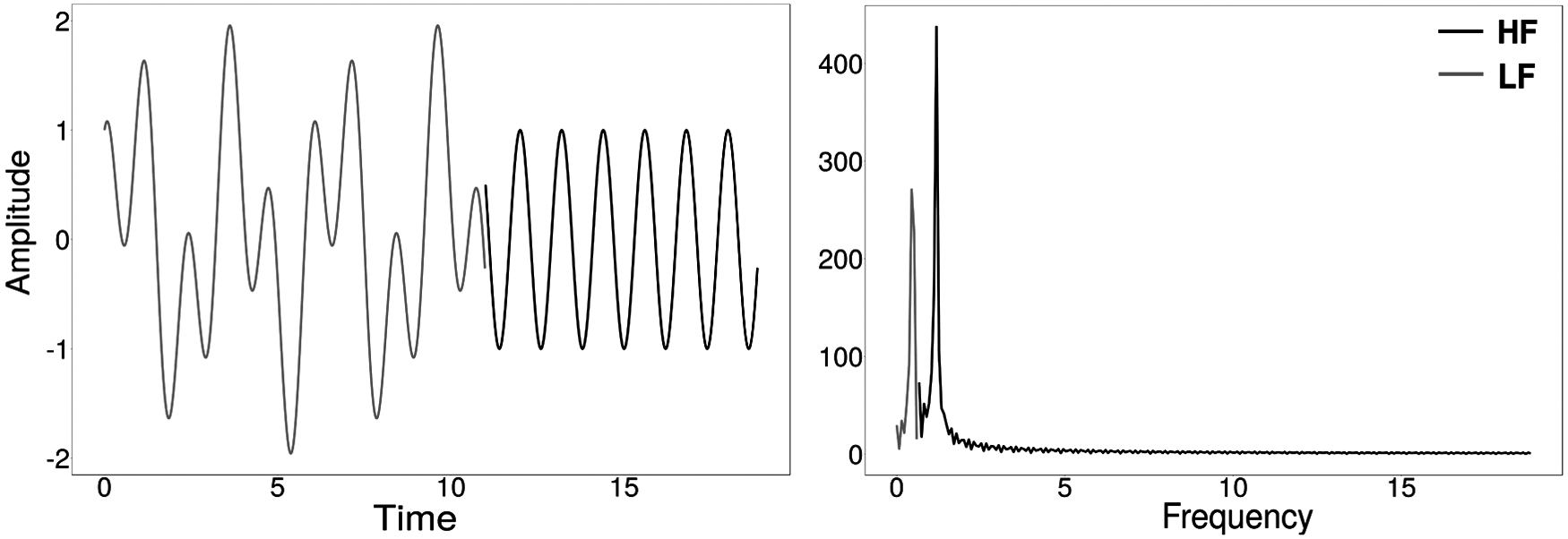
Even though the Fourier transform is a powerful tool for signal analysis and function approximation, it has some drawbacks. The most important caveat is the lack of a direct association between time and frequency domain. That is, the transform offers collective information about the frequencies in the original signal while losing information on the time locations of these frequencies. This property is referred to as time–frequency localization in the literature. Figure 1 shows the following signal:
\documentclass{aastex}\usepackage{amsbsy}\usepackage{amsfonts}\usepackage{amssymb}\usepackage{bm}\usepackage{mathrsfs}\usepackage{pifont}\usepackage{stmaryrd}\usepackage{textcomp}\usepackage{portland, xspace}\usepackage{amsmath, amsxtra}\usepackage{upgreek}\pagestyle{empty}\DeclareMathSizes{10}{9}{7}{6}\begin{document}
\begin{align*}
f (x) = \begin{cases} \sin \left({2 \pi t}/3 \right) & t \in
\left[0 , 7 \pi/2\right]\\
\cos \left(5 \pi t/3\right) & t \in \left(7 \pi/2, 6 \pi \right]\\
0 & {o.w} \\
\end{cases}. \tag{2}
\end{align*}
\end{document}
Lack of time–frequency localization with Fourier transforms. There is a transition (LF to HF) in frequency at ∼11 seconds. The transform identified the presence of two frequency components but missed the location where the transition occurred. HF, high frequency; LF, low frequency.
Many methods (Allen and Rabiner, 1977; Nawab et al., 1983; Almeida, 1994) have been suggested in the past to resolve this problem (Fig. 1). Some of them include the Windowed Fourier transform and the short time Fourier transform. Improvements were necessary, as in many applications, time–frequency localization is a desirable property in feature extraction.
2.2. Wavelet transform
Wavelet transforms, by definition, naturally provide time–frequency localization (Daubechies, 1990) and serve as a better alternative to Fourier transforms in many signal processing algorithms. Wavelet transforms are desired in feature extraction methods (Pittner and Kamarthi, 1999; Bruce et al., 2002; Subasi, 2007) as they detect sharp changes in both time and frequency while offering sparsity. The proposed method improves the approach in Hoang et al. (2015) using these desirable properties of wavelet transforms.
The wavelet transform of a function is defined as
\documentclass{aastex}\usepackage{amsbsy}\usepackage{amsfonts}\usepackage{amssymb}\usepackage{bm}\usepackage{mathrsfs}\usepackage{pifont}\usepackage{stmaryrd}\usepackage{textcomp}\usepackage{portland, xspace}\usepackage{amsmath, amsxtra}\usepackage{upgreek}\pagestyle{empty}\DeclareMathSizes{10}{9}{7}{6}\begin{document}
\begin{align*}
f ( x ) = \mathop \sum \limits_{k = 1}^{{M_0}} {V_{{j_0}k}}{ \phi _{0k}} ( x ) + \mathop \sum \limits_{j = {j_0}}^ \infty \mathop \sum \limits_{k = 1}^{{M_j}} {W_{jk}}{ \psi _{jk}} ( x ) , \tag{3}
\end{align*}
\end{document}
where \documentclass{aastex}\usepackage{amsbsy}\usepackage{amsfonts}\usepackage{amssymb}\usepackage{bm}\usepackage{mathrsfs}\usepackage{pifont}\usepackage{stmaryrd}\usepackage{textcomp}\usepackage{portland, xspace}\usepackage{amsmath, amsxtra}\usepackage{upgreek}\pagestyle{empty}\DeclareMathSizes{10}{9}{7}{6}\begin{document}
$$\psi$$
\end{document} and \documentclass{aastex}\usepackage{amsbsy}\usepackage{amsfonts}\usepackage{amssymb}\usepackage{bm}\usepackage{mathrsfs}\usepackage{pifont}\usepackage{stmaryrd}\usepackage{textcomp}\usepackage{portland, xspace}\usepackage{amsmath, amsxtra}\usepackage{upgreek}\pagestyle{empty}\DeclareMathSizes{10}{9}{7}{6}\begin{document}
$$\phi$$
\end{document} are wavelet basis functions. However, the sum in Equation (3) (Percival and Walden, 2006) is typically finite with discretized functions. Ultimately, the DWT will offer a set of coefficients with specific features at various levels (resolutions) of decomposition. The values of detail coefficients (di) and the smooth coefficients (ci) reveal sharp changes (high frequency components) and smoothness (low frequency components), respectively. That is \documentclass{aastex}\usepackage{amsbsy}\usepackage{amsfonts}\usepackage{amssymb}\usepackage{bm}\usepackage{mathrsfs}\usepackage{pifont}\usepackage{stmaryrd}\usepackage{textcomp}\usepackage{portland, xspace}\usepackage{amsmath, amsxtra}\usepackage{upgreek}\pagestyle{empty}\DeclareMathSizes{10}{9}{7}{6}\begin{document}
$$\Theta = \left[ {{d_i} , {s_i}} \right] ,$$
\end{document} where \documentclass{aastex}\usepackage{amsbsy}\usepackage{amsfonts}\usepackage{amssymb}\usepackage{bm}\usepackage{mathrsfs}\usepackage{pifont}\usepackage{stmaryrd}\usepackage{textcomp}\usepackage{portland, xspace}\usepackage{amsmath, amsxtra}\usepackage{upgreek}\pagestyle{empty}\DeclareMathSizes{10}{9}{7}{6}\begin{document}
$$i = 0 , 1 , \ldots ( J - 1 )$$
\end{document} such that \documentclass{aastex}\usepackage{amsbsy}\usepackage{amsfonts}\usepackage{amssymb}\usepackage{bm}\usepackage{mathrsfs}\usepackage{pifont}\usepackage{stmaryrd}\usepackage{textcomp}\usepackage{portland, xspace}\usepackage{amsmath, amsxtra}\usepackage{upgreek}\pagestyle{empty}\DeclareMathSizes{10}{9}{7}{6}\begin{document}
$$N{ = 2^J}$$
\end{document} (the length of the signal). In this study, “\documentclass{aastex}\usepackage{amsbsy}\usepackage{amsfonts}\usepackage{amssymb}\usepackage{bm}\usepackage{mathrsfs}\usepackage{pifont}\usepackage{stmaryrd}\usepackage{textcomp}\usepackage{portland, xspace}\usepackage{amsmath, amsxtra}\usepackage{upgreek}\pagestyle{empty}\DeclareMathSizes{10}{9}{7}{6}\begin{document}
$$i = 0$$
\end{document}” is the lowest level of decomposition and “J” is the topmost. Because of its construction, the smooth coefficient(s) need be retained only at the lowest level of decomposition (level zero, or level \documentclass{aastex}\usepackage{amsbsy}\usepackage{amsfonts}\usepackage{amssymb}\usepackage{bm}\usepackage{mathrsfs}\usepackage{pifont}\usepackage{stmaryrd}\usepackage{textcomp}\usepackage{portland, xspace}\usepackage{amsmath, amsxtra}\usepackage{upgreek}\pagestyle{empty}\DeclareMathSizes{10}{9}{7}{6}\begin{document}
$${j_0} \in \{ 1 , 2 , \ldots , ( J - 1 ) \} $$
\end{document}). Thus, the coefficient vector obtained from Equation (3) reduces to \documentclass{aastex}\usepackage{amsbsy}\usepackage{amsfonts}\usepackage{amssymb}\usepackage{bm}\usepackage{mathrsfs}\usepackage{pifont}\usepackage{stmaryrd}\usepackage{textcomp}\usepackage{portland, xspace}\usepackage{amsmath, amsxtra}\usepackage{upgreek}\pagestyle{empty}\DeclareMathSizes{10}{9}{7}{6}\begin{document}
$$\Theta = \left[ {{d_i} , {s_0}} \right].$$
\end{document} At the \documentclass{aastex}\usepackage{amsbsy}\usepackage{amsfonts}\usepackage{amssymb}\usepackage{bm}\usepackage{mathrsfs}\usepackage{pifont}\usepackage{stmaryrd}\usepackage{textcomp}\usepackage{portland, xspace}\usepackage{amsmath, amsxtra}\usepackage{upgreek}\pagestyle{empty}\DeclareMathSizes{10}{9}{7}{6}\begin{document}
$${i^{th}}$$
\end{document} level of decomposition, the length of di is \documentclass{aastex}\usepackage{amsbsy}\usepackage{amsfonts}\usepackage{amssymb}\usepackage{bm}\usepackage{mathrsfs}\usepackage{pifont}\usepackage{stmaryrd}\usepackage{textcomp}\usepackage{portland, xspace}\usepackage{amsmath, amsxtra}\usepackage{upgreek}\pagestyle{empty}\DeclareMathSizes{10}{9}{7}{6}\begin{document}
$$N{ / 2^{J - i}} \equiv {2^i}$$
\end{document} and \documentclass{aastex}\usepackage{amsbsy}\usepackage{amsfonts}\usepackage{amssymb}\usepackage{bm}\usepackage{mathrsfs}\usepackage{pifont}\usepackage{stmaryrd}\usepackage{textcomp}\usepackage{portland, xspace}\usepackage{amsmath, amsxtra}\usepackage{upgreek}\pagestyle{empty}\DeclareMathSizes{10}{9}{7}{6}\begin{document}
$$i = 0 , \ 1 , \ldots ( J - 1 )$$
\end{document}. The function in Equation (2) and the first level of its wavelet decomposition are shown in Figure 2. It can be seen that the time at which there is a transition in frequency is captured by the transform. The first (upper) level captures high-frequency changes in the signal.
Wavelet coefficients of a signal composed of high- and low-frequency components.
The signal is smooth everywhere except for the transition point. This explains the sparsity of the spectrum at the first level. Low frequency changes are captured by smooth coefficients in lower levels of the decomposition. The coefficients obtained from DWT satisfies Parseval's theorem (Oppenheim and Schafer, 2009) similar to Fourier coefficients. That is,
\documentclass{aastex}\usepackage{amsbsy}\usepackage{amsfonts}\usepackage{amssymb}\usepackage{bm}\usepackage{mathrsfs}\usepackage{pifont}\usepackage{stmaryrd}\usepackage{textcomp}\usepackage{portland, xspace}\usepackage{amsmath, amsxtra}\usepackage{upgreek}\pagestyle{empty}\DeclareMathSizes{10}{9}{7}{6}\begin{document}
\begin{align*}
\mathop \sum \limits_{i = 1}^n \vert x ( n{ ) \vert ^2} = \mathop \sum \limits_{i = 1}^{J - 1} \mathop \sum \limits_{j = 1}^{{n_i}} d_{ij}^2 + \mathop \sum \limits_{j = 1}^{{n_0}} s_{0j}^2 , \tag{4}
\end{align*}
\end{document}
We define indicator sequences for the four nucleotide bases, adenine (A), guanine (G), cytosine (C), and thiamine (T). For example, the sequence AGTC has a corresponding position vector of nucleotide A as 1000. Without loss of generality, we construct a moment of wavelet power spectrum of an indicator UA. Define the length of UA as NA, then using Equation (4) we obtain
\documentclass{aastex}\usepackage{amsbsy}\usepackage{amsfonts}\usepackage{amssymb}\usepackage{bm}\usepackage{mathrsfs}\usepackage{pifont}\usepackage{stmaryrd}\usepackage{textcomp}\usepackage{portland, xspace}\usepackage{amsmath, amsxtra}\usepackage{upgreek}\pagestyle{empty}\DeclareMathSizes{10}{9}{7}{6}\begin{document}
\begin{align*}
\mathop \sum \limits_{i = 1}^n \vert {U_A} ( n{ ) \vert ^2} = {N_A} \tag{5}
\end{align*}
\end{document}\documentclass{aastex}\usepackage{amsbsy}\usepackage{amsfonts}\usepackage{amssymb}\usepackage{bm}\usepackage{mathrsfs}\usepackage{pifont}\usepackage{stmaryrd}\usepackage{textcomp}\usepackage{portland, xspace}\usepackage{amsmath, amsxtra}\usepackage{upgreek}\pagestyle{empty}\DeclareMathSizes{10}{9}{7}{6}\begin{document}
\begin{align*}
\rightarrow {N_A} = \mathop \sum \limits_{i = 1}^{J - 1} \mathop \sum \limits_{j = 1}^{{n_i}} d_{ij}^2 + \mathop \sum \limits_{j = 1}^{{n_0}} s_{0j}^2. \tag{6}
\end{align*}
\end{document}
To preserve the essence of sequence information in the first few moments, the \documentclass{aastex}\usepackage{amsbsy}\usepackage{amsfonts}\usepackage{amssymb}\usepackage{bm}\usepackage{mathrsfs}\usepackage{pifont}\usepackage{stmaryrd}\usepackage{textcomp}\usepackage{portland, xspace}\usepackage{amsmath, amsxtra}\usepackage{upgreek}\pagestyle{empty}\DeclareMathSizes{10}{9}{7}{6}\begin{document}
$${n^{th}}$$
\end{document} moment is normalized with \documentclass{aastex}\usepackage{amsbsy}\usepackage{amsfonts}\usepackage{amssymb}\usepackage{bm}\usepackage{mathrsfs}\usepackage{pifont}\usepackage{stmaryrd}\usepackage{textcomp}\usepackage{portland, xspace}\usepackage{amsmath, amsxtra}\usepackage{upgreek}\pagestyle{empty}\DeclareMathSizes{10}{9}{7}{6}\begin{document}
$$\alpha _{{N_A}}^{ ( n ) }$$
\end{document}. We define the normalized moment as
\documentclass{aastex}\usepackage{amsbsy}\usepackage{amsfonts}\usepackage{amssymb}\usepackage{bm}\usepackage{mathrsfs}\usepackage{pifont}\usepackage{stmaryrd}\usepackage{textcomp}\usepackage{portland, xspace}\usepackage{amsmath, amsxtra}\usepackage{upgreek}\pagestyle{empty}\DeclareMathSizes{10}{9}{7}{6}\begin{document}
\begin{align*}
M_{{N_A}}^{ ( n ) } = \alpha _{{N_A}}^{ ( n ) } \mathop \sum \limits_{k = 1}^N W_k^{ ( A ) n}. \tag{8}
\end{align*}
\end{document}
The normalization constant \documentclass{aastex}\usepackage{amsbsy}\usepackage{amsfonts}\usepackage{amssymb}\usepackage{bm}\usepackage{mathrsfs}\usepackage{pifont}\usepackage{stmaryrd}\usepackage{textcomp}\usepackage{portland, xspace}\usepackage{amsmath, amsxtra}\usepackage{upgreek}\pagestyle{empty}\DeclareMathSizes{10}{9}{7}{6}\begin{document}
$$\alpha _{{N_A}}^{ ( n ) }$$
\end{document} is set as \documentclass{aastex}\usepackage{amsbsy}\usepackage{amsfonts}\usepackage{amssymb}\usepackage{bm}\usepackage{mathrsfs}\usepackage{pifont}\usepackage{stmaryrd}\usepackage{textcomp}\usepackage{portland, xspace}\usepackage{amsmath, amsxtra}\usepackage{upgreek}\pagestyle{empty}\DeclareMathSizes{10}{9}{7}{6}\begin{document}
$$= {1 \mathord{ \left/ { \vphantom {1 {N_A^{n - 1}}}} \right. } {N_A^{n - 1}}}$$
\end{document} for the following reasons. With a normalization constant,
\documentclass{aastex}\usepackage{amsbsy}\usepackage{amsfonts}\usepackage{amssymb}\usepackage{bm}\usepackage{mathrsfs}\usepackage{pifont}\usepackage{stmaryrd}\usepackage{textcomp}\usepackage{portland, xspace}\usepackage{amsmath, amsxtra}\usepackage{upgreek}\pagestyle{empty}\DeclareMathSizes{10}{9}{7}{6}\begin{document}
\begin{align*}
M_ { { N_A } } ^ { ( n ) } = \frac { 1 } { { N_A^ { n - 1 } } } \mathop \sum \limits_ { k = 1 } ^N W_k^ { ( A ) n } \tag { 9 }
\end{align*}
\end{document}\documentclass{aastex}\usepackage{amsbsy}\usepackage{amsfonts}\usepackage{amssymb}\usepackage{bm}\usepackage{mathrsfs}\usepackage{pifont}\usepackage{stmaryrd}\usepackage{textcomp}\usepackage{portland, xspace}\usepackage{amsmath, amsxtra}\usepackage{upgreek}\pagestyle{empty}\DeclareMathSizes{10}{9}{7}{6}\begin{document}
\begin{align*}
\quad \quad = { \frac { { N_A } } { N_A^n } } \mathop \sum \limits_ { k = 1 } ^N W_k^ { ( A ) n } \tag { 10 }
\end{align*}
\end{document}\documentclass{aastex}\usepackage{amsbsy}\usepackage{amsfonts}\usepackage{amssymb}\usepackage{bm}\usepackage{mathrsfs}\usepackage{pifont}\usepackage{stmaryrd}\usepackage{textcomp}\usepackage{portland, xspace}\usepackage{amsmath, amsxtra}\usepackage{upgreek}\pagestyle{empty}\DeclareMathSizes{10}{9}{7}{6}\begin{document}
\begin{align*}
\quad \quad = { N_A } \mathop \sum \limits_ { k = 1 } ^N { \left( { { \frac { W_k^ { ( A ) } } { { N_A } } } } \right) ^n } . \tag { 11 }
\end{align*}
\end{document}
By defining a normalization constant, we satisfy \documentclass{aastex}\usepackage{amsbsy}\usepackage{amsfonts}\usepackage{amssymb}\usepackage{bm}\usepackage{mathrsfs}\usepackage{pifont}\usepackage{stmaryrd}\usepackage{textcomp}\usepackage{portland, xspace}\usepackage{amsmath, amsxtra}\usepackage{upgreek}\pagestyle{empty}\DeclareMathSizes{10}{9}{7}{6}\begin{document}
$$M_{{N_A}}^{ ( n ) } = {N_A}$$
\end{document} and the moments rapidly converge to 0 as \documentclass{aastex}\usepackage{amsbsy}\usepackage{amsfonts}\usepackage{amssymb}\usepackage{bm}\usepackage{mathrsfs}\usepackage{pifont}\usepackage{stmaryrd}\usepackage{textcomp}\usepackage{portland, xspace}\usepackage{amsmath, amsxtra}\usepackage{upgreek}\pagestyle{empty}\DeclareMathSizes{10}{9}{7}{6}\begin{document}
$$\mathop { \lim } \limits_ { n \to \infty } { \left( { { \frac { W_k^ { ( A ) } } { { N_A } } } } \right) ^n } \to 0$$
\end{document}. In Equation (9), if a partial DWT decomposition is considered up to level “\documentclass{aastex}\usepackage{amsbsy}\usepackage{amsfonts}\usepackage{amssymb}\usepackage{bm}\usepackage{mathrsfs}\usepackage{pifont}\usepackage{stmaryrd}\usepackage{textcomp}\usepackage{portland, xspace}\usepackage{amsmath, amsxtra}\usepackage{upgreek}\pagestyle{empty}\DeclareMathSizes{10}{9}{7}{6}\begin{document}
$$\ell$$
\end{document}” such that \documentclass{aastex}\usepackage{amsbsy}\usepackage{amsfonts}\usepackage{amssymb}\usepackage{bm}\usepackage{mathrsfs}\usepackage{pifont}\usepackage{stmaryrd}\usepackage{textcomp}\usepackage{portland, xspace}\usepackage{amsmath, amsxtra}\usepackage{upgreek}\pagestyle{empty}\DeclareMathSizes{10}{9}{7}{6}\begin{document}
$$\ell$$
\end{document} mod \documentclass{aastex}\usepackage{amsbsy}\usepackage{amsfonts}\usepackage{amssymb}\usepackage{bm}\usepackage{mathrsfs}\usepackage{pifont}\usepackage{stmaryrd}\usepackage{textcomp}\usepackage{portland, xspace}\usepackage{amsmath, amsxtra}\usepackage{upgreek}\pagestyle{empty}\DeclareMathSizes{10}{9}{7}{6}\begin{document}
$${ \kern 1pt} 2 = 0$$
\end{document}, there exists a relationship between the sum of the smooth coefficients and NA. In general, the sum of the smooth coefficients is proportional to NA. If \documentclass{aastex}\usepackage{amsbsy}\usepackage{amsfonts}\usepackage{amssymb}\usepackage{bm}\usepackage{mathrsfs}\usepackage{pifont}\usepackage{stmaryrd}\usepackage{textcomp}\usepackage{portland, xspace}\usepackage{amsmath, amsxtra}\usepackage{upgreek}\pagestyle{empty}\DeclareMathSizes{10}{9}{7}{6}\begin{document}
$$\ell$$
\end{document} mod \documentclass{aastex}\usepackage{amsbsy}\usepackage{amsfonts}\usepackage{amssymb}\usepackage{bm}\usepackage{mathrsfs}\usepackage{pifont}\usepackage{stmaryrd}\usepackage{textcomp}\usepackage{portland, xspace}\usepackage{amsmath, amsxtra}\usepackage{upgreek}\pagestyle{empty}\DeclareMathSizes{10}{9}{7}{6}\begin{document}
$${ \kern 1pt} 2 = 0$$
\end{document}, then the constant of proportionality is 1. It is not the case if \documentclass{aastex}\usepackage{amsbsy}\usepackage{amsfonts}\usepackage{amssymb}\usepackage{bm}\usepackage{mathrsfs}\usepackage{pifont}\usepackage{stmaryrd}\usepackage{textcomp}\usepackage{portland, xspace}\usepackage{amsmath, amsxtra}\usepackage{upgreek}\pagestyle{empty}\DeclareMathSizes{10}{9}{7}{6}\begin{document}
$$\ell$$
\end{document} mod \documentclass{aastex}\usepackage{amsbsy}\usepackage{amsfonts}\usepackage{amssymb}\usepackage{bm}\usepackage{mathrsfs}\usepackage{pifont}\usepackage{stmaryrd}\usepackage{textcomp}\usepackage{portland, xspace}\usepackage{amsmath, amsxtra}\usepackage{upgreek}\pagestyle{empty}\DeclareMathSizes{10}{9}{7}{6}\begin{document}
$${ \kern 1pt} 2 = 1$$
\end{document}. Therefore,
\documentclass{aastex}\usepackage{amsbsy}\usepackage{amsfonts}\usepackage{amssymb}\usepackage{bm}\usepackage{mathrsfs}\usepackage{pifont}\usepackage{stmaryrd}\usepackage{textcomp}\usepackage{portland, xspace}\usepackage{amsmath, amsxtra}\usepackage{upgreek}\pagestyle{empty}\DeclareMathSizes{10}{9}{7}{6}\begin{document}
\begin{align*}
W_k^{ ( A ) } = \mathop \sum \limits_{i = 1}^{J - 1} \mathop \sum \limits_{j = 1}^{{n_i}} d_{ij}^2 + \mathop \sum \limits_{j = 1}^{{n_ \ell }} s_{ \ell j}^2 ,
\end{align*}
\end{document}
If the smooth coefficients are removed in calculating the moments, then only the details (local features) of the signal are captured. Define
\documentclass{aastex}\usepackage{amsbsy}\usepackage{amsfonts}\usepackage{amssymb}\usepackage{bm}\usepackage{mathrsfs}\usepackage{pifont}\usepackage{stmaryrd}\usepackage{textcomp}\usepackage{portland, xspace}\usepackage{amsmath, amsxtra}\usepackage{upgreek}\pagestyle{empty}\DeclareMathSizes{10}{9}{7}{6}\begin{document}
\begin{align*}
V_k^{ ( A ) } = W_k^{ ( A ) } - \mathop \sum \limits_{j = 1}^{{n_ \ell }} s_{ \ell j}^2.
\end{align*}
\end{document}
Then, the \documentclass{aastex}\usepackage{amsbsy}\usepackage{amsfonts}\usepackage{amssymb}\usepackage{bm}\usepackage{mathrsfs}\usepackage{pifont}\usepackage{stmaryrd}\usepackage{textcomp}\usepackage{portland, xspace}\usepackage{amsmath, amsxtra}\usepackage{upgreek}\pagestyle{empty}\DeclareMathSizes{10}{9}{7}{6}\begin{document}
$${n^{th}}$$
\end{document} moment with a normalization constant \documentclass{aastex}\usepackage{amsbsy}\usepackage{amsfonts}\usepackage{amssymb}\usepackage{bm}\usepackage{mathrsfs}\usepackage{pifont}\usepackage{stmaryrd}\usepackage{textcomp}\usepackage{portland, xspace}\usepackage{amsmath, amsxtra}\usepackage{upgreek}\pagestyle{empty}\DeclareMathSizes{10}{9}{7}{6}\begin{document}
$$\beta _{{N_A}}^{ ( n ) } = {1 \Big/ {{{ \Big ( {{N_A} - 2^{ - \ell / 2}{N_A}} \Big ) }^{n - 1}}}}$$
\end{document} can be defined as
\documentclass{aastex}\usepackage{amsbsy}\usepackage{amsfonts}\usepackage{amssymb}\usepackage{bm}\usepackage{mathrsfs}\usepackage{pifont}\usepackage{stmaryrd}\usepackage{textcomp}\usepackage{portland, xspace}\usepackage{amsmath, amsxtra}\usepackage{upgreek}\pagestyle{empty}\DeclareMathSizes{10}{9}{7}{6}\begin{document}
\begin{align*}
M_{{N_A}}^{ ( n ) } = \beta _{{N_A}}^{ ( n ) } \mathop \sum \limits_{k = 1}^N V_k^{ ( A ) n}.
\end{align*}
\end{document}
The rationale for the normalization constant based on the expression for \documentclass{aastex}\usepackage{amsbsy}\usepackage{amsfonts}\usepackage{amssymb}\usepackage{bm}\usepackage{mathrsfs}\usepackage{pifont}\usepackage{stmaryrd}\usepackage{textcomp}\usepackage{portland, xspace}\usepackage{amsmath, amsxtra}\usepackage{upgreek}\pagestyle{empty}\DeclareMathSizes{10}{9}{7}{6}\begin{document}
$$V_k^{ ( A ) }$$
\end{document} is as follows.
\documentclass{aastex}\usepackage{amsbsy}\usepackage{amsfonts}\usepackage{amssymb}\usepackage{bm}\usepackage{mathrsfs}\usepackage{pifont}\usepackage{stmaryrd}\usepackage{textcomp}\usepackage{portland, xspace}\usepackage{amsmath, amsxtra}\usepackage{upgreek}\pagestyle{empty}\DeclareMathSizes{10}{9}{7}{6}\begin{document}
\begin{align*} M_ { { N_A } } ^ { ( n ) } & = \frac { 1 } { { { { \big ( { { N_A } - 2^ { - \ell / 2 } { N_A } } \big ) } ^ { n - 1 } } } } \mathop \sum \limits_ { k = 1 } ^N V_k^ { ( A ) n } \\ & = { \frac { { N_A } } { N_A^n { { \big ( { 1 - 2^ { - \ell / 2 } \big ) } ^n } } } } \mathop \sum \limits_ { k = 1 } ^N V_k^ { ( A ) n } . \end{align*}
\end{document}
According to the analysis of the examined data, the first three moments are sufficient for clustering. Therefore, each genome sequence is represented as a 12-dimensional numerical vector
\documentclass{aastex}\usepackage{amsbsy}\usepackage{amsfonts}\usepackage{amssymb}\usepackage{bm}\usepackage{mathrsfs}\usepackage{pifont}\usepackage{stmaryrd}\usepackage{textcomp}\usepackage{portland, xspace}\usepackage{amsmath, amsxtra}\usepackage{upgreek}\pagestyle{empty}\DeclareMathSizes{10}{9}{7}{6}\begin{document}
\begin{align*}
\left( {M_{{N_A}}^{ ( 1 ) } , M_{{N_C}}^{ ( 1 ) } , M_{{N_G}}^{ ( 1 ) } , M_{{N_T}}^{ ( 1 ) } , M_{{N_A}}^{ ( 2 ) } , M_{{N_C}}^{ ( 2 ) } , M_{{N_G}}^{ ( 2 ) } , M_{{N_T}}^{ ( 2 ) } , M_{{N_A}}^{ ( 3 ) } , M_{{N_C}}^{ ( 3 ) } , M_{{N_G}}^{ ( 3 ) } , M_{{N_T}}^{ ( 3 ) }} \right).
\end{align*}
\end{document}
Furthermore, mutual distances between two vectors are calculated, and a distance-based tree is constructed for clustering the genome sequences. The proposed approach is named as wavelet spectrum moments (WSMs) method.
3. Results
WSM is tested on six benchmark data sets, which has been used in Hoang et al. (2015). For each data set, genome sequences are transformed into 12-dimensional vector, their mutual distances are calculated, and then a distance-based phylogenetic tree is built using the unweighted pair group method with arithmetic mean (UPGMA) (Sokal and Michener, 1958) or neighbor-joining (Saitou and Nei, 1987) methods for clustering. We applied seven wavelet families, including Daubechies, Coiflets, Symlets, Fejer-Korovkin filters, Discrete Meyer, Biorthogonal, and Reverse Biorthogonal wavelets provided by Matlab (2016) for DWT and construct trees by Mega 7 (Kumar et al., 2016). The sequence lengths of these data sets vary from few hundreds to millions of nucleotides. Under the same computing condition (Intel Core i7 CPU 2.40 GHz and 8 GB RAM) as Hoang et al. (2015), we compare our method with PS-M, which is a new alignment-free method developed by Hoang et al. (2015) and has been shown running faster than k-mer (Vinga and Almeida, 2003), MAFFT (Katoh et al., 2002), and ClustalW (Larkin et al., 2007), in terms of computational time.
3.1. Mammals
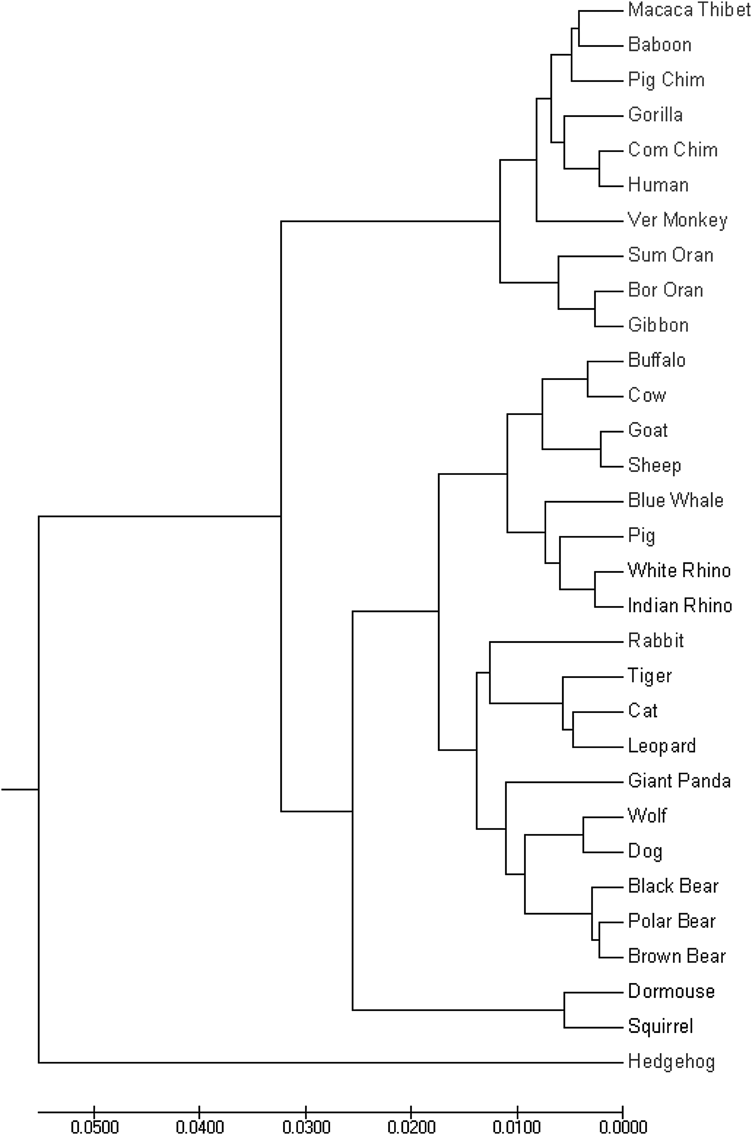
The first data set consists of 31 mammalian mitochondrial DNA sequences from GenBank with sequence lengths varying from 16,300 to 17,500 nucleotides. The UPGMA tree based on WSMs with bior3.3 wavelet correctly clusters the 31 genomes into 7 biological classes: Primates, Cetacea and Artiodactyla, Perissodactyla, Rodentia, Lagomorpha, Carnivore, and Erinaceomorpha (Fig. 3) using less running time than PS-M (Table 1).
The UPGMA phylogenetic tree of the mammalian mitochondrial genomes by the proposed method with bior3.3 wavelet. UPGMA.
Computational time Comparison
Data sets
WSM
PS-M
Mammals
1.39
4
Influenza A
0.79
0.6
HRV
2.59
5
Coronavirus
1.82
6
Bacteria
33.58
581
HRVs, human rhinoviruses; PS-M, power spectrum moments; WSMs, wavelet spectrum moments.
3.2. Influenza A viruses
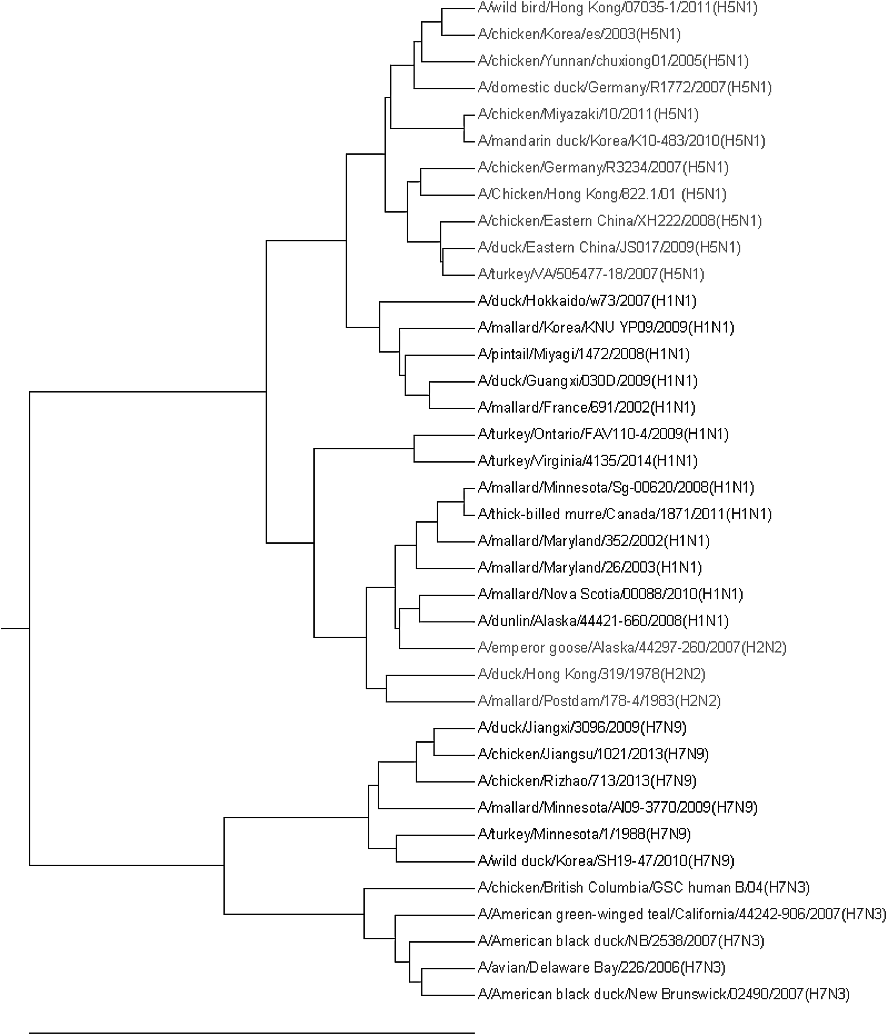
Influenza A viruses are single-stranded RNA viruses with eight segments. Among these segments, segment 4 encoding for hemagglutinin (H) protein and segment 6 encoding neuraminidase (N) protein determine subtypes of influenza A viruses (Webster et al., 1992). There are 18 H serotypes (H1–H18) and 11 N (N1–N11) serotypes. We test the proposed WSMs method by clustering segment 6 of H1N1, H2N2, H5N1, H7N3, and H7N9 subtypes of avian influenza A viruses, which were selected and examined in Hoang et al. (2015). The UPGMA tree based on WSMs with rbio3.7 wavelet clusters the influenza A viruses correctly into five subtypes (Fig. 4).
The UPGMA phylogenetic tree of the 38 influenza A viral genomes by the proposed method with the rbio3.7 wavelet.
3.3. Human rhinovirus
To test the efficiency, WSMs method is applied to a data set including 116 genome sequences of human rhinoviruses (HRVs). HRVs are associated with respiratory diseases, and the predominant cause of common cold (Jacobs et al., 2013). Our data consist of three groups: HRV-A, HRV-B, and HRV-C of 113 genomes and three out-group sequences of HEV-C (Palmenberg et al., 2009). The neighbor-joining tree based on WSMs with Coif2 wavelet correctly clusters the three groups of HRV and distinguishes the out-group HEV-C (Fig. 5) with only 2.59 seconds running time, which is about a half of PS-M (Table 1).
The neighbor-joining phylogenetic tree of the human rhinovirus genomes by the proposed method with Coif2 wavelet.
3.4. Coronavirus
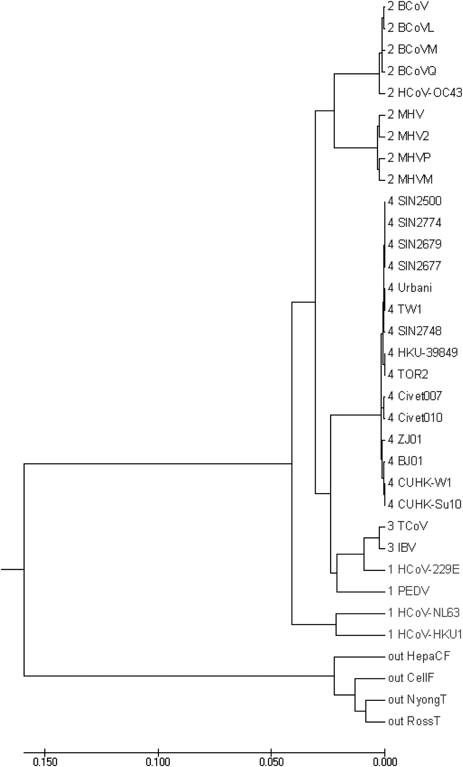
Coronaviruses, a genus of the Coronaviridae family, can cause a variety of severe diseases in respiratory and gastrointestinal tract of mammals and birds. Therefore, it is important to identify the species of coronaviruses, especially for human coronaviruses (van der Hoek et al., 2004; Abdul-Rasool and Fielding, 2010), which are important and have been extensively studied so far. We cluster the set of 30 coronaviruses and 4 out-group noncoronavirus sequences using the WSM method. WSM clusters these coronavirus genomes into four groups correctly (Fig. 6).
The UPGMA phylogenetic tree of the coronavirus genomes by the proposed method using bior3.9 wavelet.
3.5. Bacteria
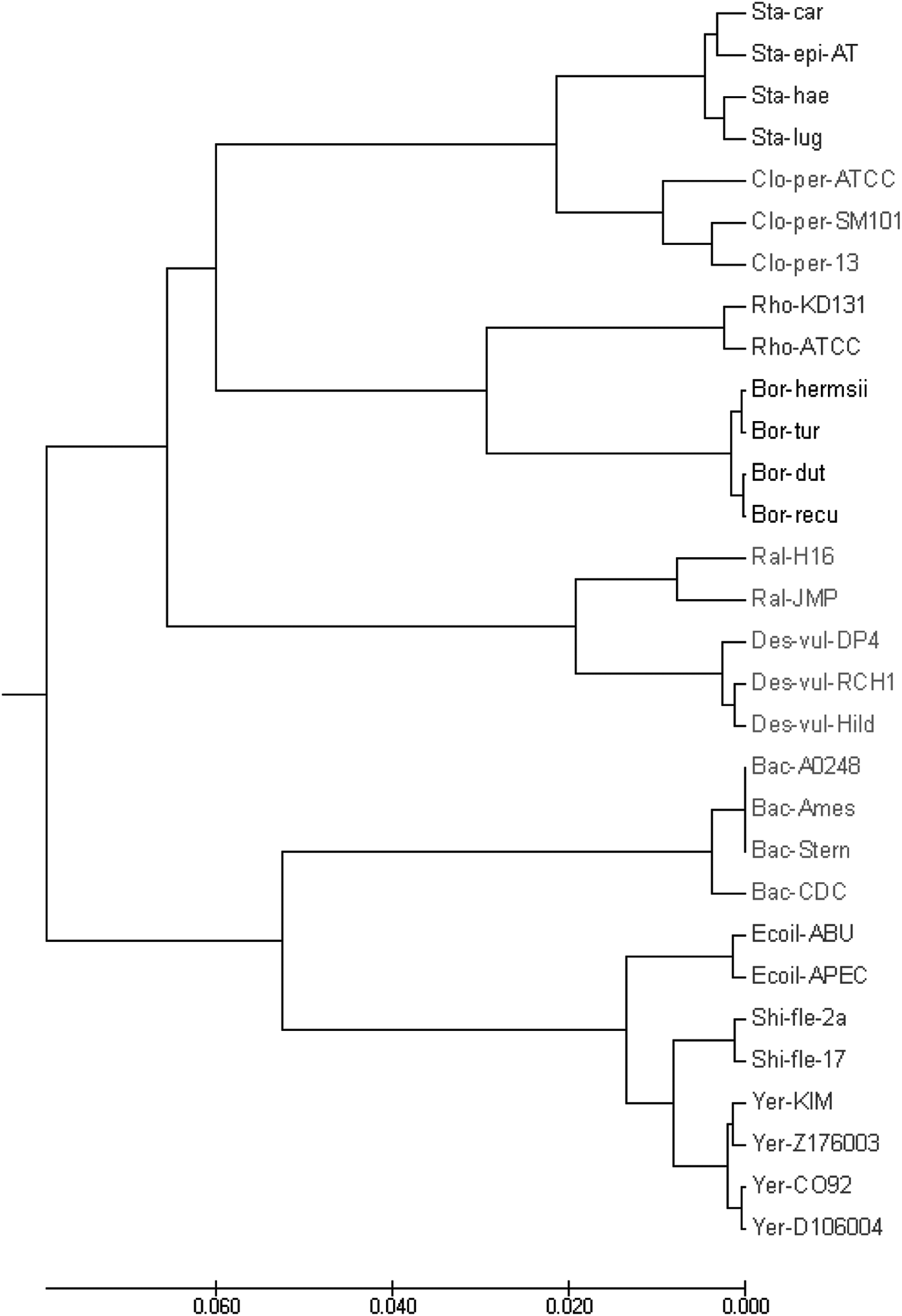
Methods such as multiple sequence alignment cannot deal with bacteria genomes consisting of millions of base pairs (Hoang et al., 2015). Therefore, we test WSMs on the set of 30 bacterial genomes, including 8 families: Enterobacteriaceae, Bacillaceae, Rhodobacteraceae, Spirochaetaceae, Desulfovibrionaceae, Clostridiaceae, Burkholderiaceae, and Staphylococcaceae. Most of the data have a length between 3 and 5 million base pairs. The UPGMA phylogenetic tree (Fig. 7) based on WSMs with bior5.5 wavelet correctly clusters the genomes into eight groups using only 33.58 seconds, which is 5.78% of the running time of PS-M (Table 1).
The UPGMA phylogenetic tree of the bacteria species by the proposed method using bior5.5 wavelet.
4. Discussion
The selection of wavelets depends on data. In our experiments, biorthogonal wavelets are useful in multiple data sets and they can be computed quickly (Keinert, 1995). The computational complexity in obtaining a DWT of signal of length N is \documentclass{aastex}\usepackage{amsbsy}\usepackage{amsfonts}\usepackage{amssymb}\usepackage{bm}\usepackage{mathrsfs}\usepackage{pifont}\usepackage{stmaryrd}\usepackage{textcomp}\usepackage{portland, xspace}\usepackage{amsmath, amsxtra}\usepackage{upgreek}\pagestyle{empty}\DeclareMathSizes{10}{9}{7}{6}\begin{document}
$$O ( N )$$
\end{document}, whereas the complexity of FFT is \documentclass{aastex}\usepackage{amsbsy}\usepackage{amsfonts}\usepackage{amssymb}\usepackage{bm}\usepackage{mathrsfs}\usepackage{pifont}\usepackage{stmaryrd}\usepackage{textcomp}\usepackage{portland, xspace}\usepackage{amsmath, amsxtra}\usepackage{upgreek}\pagestyle{empty}\DeclareMathSizes{10}{9}{7}{6}\begin{document}
$$O ( N \log ( N ) )$$
\end{document} (Beylkin et al., 1991; Wu et al., 2000). Consequently, the computational time of WSM is much less than PS-M. Particularly for the bacteria genomes data, none of the popular methods such as k-mer, MAFFT, and ClustalW could cluster them well (Hoang et al., 2015). Even though PS-M could result in a reasonable tree, it runs 17.3 times longer than WSMs. Based on the experimental results, the proposed WSMs method is an efficient and effective approach for real-time genome comparison.
Footnotes
Acknowledgments
This research is supported by In-House grant of the University of Central Florida. We thank Dr. Tung Hoang for helping us program the Matlab code.
Author Disclosure Statement
No competing financial interests exist.
References
1.
Abdul-RasoolS., and FieldingB.C.2010. Understanding human coronavirus HCoV-NL63. Open Virol. J., 4, 76–84.
2.
AllenJ.B., and RabinerL.R.1977. A unified approach to short-time Fourier analysis and synthesis. Proc. IEEE. 65, 1558–1564.
3.
AlmeidaL.B.1994. The fractional Fourier transform and time-frequency representations. IEEE Trans. Sig. Process. 42, 3084–3091.
4.
AnastassiouD.2000. Frequency-domain analysis of biomolecular sequences. Bioinformatics. 16, 1073–1081.
5.
BeylkinG., CoifmanR., and RokhlinV.1991. Fast wavelet transforms and numerical algorithms I. Comm. Pure Appl. Math., 44, 141–183.
6.
BlaisdellB.E.1989. Average values of a dissimilarity measure not requiring sequence alignment are twice the averages of conventional mismatch counts requiring sequence alignment for a computer-generated model system. J. Mol. Evol., 29, 538–547.
7.
BlaisdellB.E.1986. A measure of the similarity of sets of sequences not requiring sequence alignment. Proc Natl Acad Sci U S A. 83, 5155–5159.
8.
BracewellR.1999. The Fourier Transform and Its Applications. McGraw-Hill Series in Electrical and Computer Engineering. New York NY.
9.
BrighamE.O.1974. The Fast Fourier Transform. Prentice-Hall, Englewood Cliffs, NJ.
10.
BruceL.M., KogerC.H., and LiJ.2002. Dimensionality reduction of hyperspectral data using discrete wavelet transform feature extraction. IEEE Trans. Geosci. Remote Sens. 40, 2331–2338.
11.
CominM., and VerzottoD.2012. Alignment-free phylogeny of whole genomes using underlying subwords. Algorithms Mol. Biol. 7, 34.
12.
DaubechiesI.1990. The wavelet transform, time-frequency localization and signal analysis. IEEE Trans. Informat. Theory. 36, 961–1005.
13.
EdgarR.C.2004. Muscle: multiple sequence alignment with high accuracy and high throughput. Nucleic Acids Res. 32, 1792–1797.
14.
HoangT., YinC., ZhengH., et al.2015. A new method to cluster DNA sequences using Fourier power spectrum. J. Theor. Biol. 372, 135–145.
15.
HuangH.H.2016. An ensemble distance measure of k-mer and Natural Vector for the phylogenetic analysis of multiple-segmented viruses. J. Theor. Biol. 398, 136–144.
16.
HuangH.H., and YuC.2016. Clustering DNA sequences using the out-of-place measure with reduced n-grams. J. Theor. Biol. 406, 61–72.
17.
HuangH.H., YuC., ZhengH., et al.2014. Global comparison of multiple-segmented viruses in 12-dimensional genome space. Mol. Phylogenet. Evol. 81, 29–36.
18.
JacobsS.E., LamsonD.M., GeorgeK.S., et al.2013. Human rhinoviruses. Clin. Microbiol. Rev. 26, 135–162.
19.
KatohK., MisawaK., KumaK., et al.2002. Mafft: a novel method for rapid multiple sequence alignment based on fast Fourier transform. Nucleic Acids Res. 30, 3059–3066.
20.
KeinertF.1995. Biorthogonal wavelets for fast matrix computations. Appl. Comput. Harmon. Anal. 1, 147–156.
21.
KooI., ZhangX., and KimS.2011. Wavelet and Fourier transforms-based spectrum similarity approaches to compound identification in gas chromatography mass spectrometry. Anal. Chem., 83, 5631–5638.
22.
KotlarD., and LavnerY.2003. Gene prediction by spectral rotation measure: a new method for identifying protein-coding regions. Genome Res. 13, 1930–1937.
23.
KumarS., StecherG., and TamuraK.2016. MEGA7: molecular evolutionary genetics analysis version 7.0 for bigger data sets. Mol. Biol. Evol. 33, 1870–1874.
24.
LarkinM.A., BlackshieldsG., BrownN., et al.2007. Clustal w and clustal x version 2.0. Bioinformatics. 23, 2947–2948.
25.
MachadoJ.T., CostaA.C., and QuelhasM.D.2011. Fractional dynamics in DNA. Commun. Nonlinear Sci. Numer. Simul., 16, 2963–2969.
26.
MaloneR.W., HomanJ., CallahanM.V.2016. Zika virus: medical countermeasure development challenges. PLoS Negl. Trop. Dis. 10, e0004530.
27.
MarraM.A., JonesS.J., AstellC.R., et al.2003. The genome sequence of the sars-associated coronavirus. Science. 300, 1399–1404.
28.
MATLAB and Statistics Toolbox Release. 2016. The MathWorks, Inc., Natick, MA.
29.
NawabS., QuatieriT., and LimJ.1983. Signal reconstruction from short-time Fourier transform magnitude. IEEE Trans. Acoust. Speech Sign. Process. 31, 986–998.
30.
OppenheimA.V., and SchaferR.W.2009. Discrete-Time Signal Processing, 3rd ed. Prentice-Hall Signal Processing Series. New Jersey.
31.
PalmenbergA.C, SpiroD., KuzmickasR., et al.2009. Sequencing and analyses of all known human rhinovirus genomes reveal structure and evolution. Science. 324, 55–59.
32.
PanditA., and SinhaS.2010. Using genomic signatures for hiv-1 sub-typing. BMC Bioinform. 11(Suppl 1), S26.
33.
PercivalD.B., and WaldenA.T.2006. Wavelet Methods for Time Series Analysis. Cambridge University Press. Cambridge, England.
34.
PittnerS., and KamarthiS.V.1999. Feature extraction from wavelet coefficients for pattern recognition tasks. IEEE Trans. Pattern Anal. Mach. Intell. 21, 83–88.
35.
SaitouN., and NeiM.1987. The neighbor-joining method: a new method for reconstructing phylogenetic trees. Mol. Biol. Evolut. 4, 406–425.
36.
SokalR., and MichenerC.1958. A statistical method for evaluating systematic relationships. Univ. Kans. Sci. Bull., 38, 1409–1438.
37.
SubasiA.2007. EEG signal classification using wavelet feature extraction and a mixture of expert model. Expert Syst. Appl. 32, 1084–1093.
38.
TiwariS., RamachandranS., BhattacharyaA., et al.1997. Prediction of probable genes by fourier analysis of genomic sequences. Bioinformatics. 13, 263–270.
39.
van der HoekL., PyrcK., JebbinkM.F., et al.2004. Identification of a new human coronavirus. Nat. Med., 10, 368–373.
40.
VingaS., and AlmeidaJ.2003. Alignment-free sequence comparison-a review. Bioinformatics. 19, 513–523.
41.
WebsterR.G., BeanW.J., and GormanO.T., et al.1992. Evolution and ecology of influenza A viruses. Microbiol. Rev., 56, 152–179.
42.
WuY.-L., AgrawalD., and AbbadiA.E.2000. A comparison of DFT and DWT based similarity search in time-series databases. Proceedings of the 9th International Conference on Information and Knowledge Management, 488–495.
43.
YauS.S.T., YuC., and HeR.2008. A protein map and its application. DNA Cell Biol. 27, 241–250.
44.
YinC., and YauS.S.2005. A fourier characteristic of coding sequences: origins and a non-fourier approximation. J. Comput. Biol. 12, 1153–1165.
45.
YinC., and YauS.S.2007. Prediction of protein coding regions by the 3-base periodicity analysis of a DNA sequence. J. Theor. Biol. 247, 687–694.
46.
YuC., DengM., and YauS.S.2011. DNA sequence comparison by a novel probabilistic method. Inf. Sci., 181, 1484–1492.
47.
YuC., HernandezT., ZhengH., et al.2013. Real time classification of viruses in 12 dimensions. PLoS One. 8, e64328.