A Computational-Based Method for Predicting Drug–Target Interactions by Using Stacked Autoencoder Deep Neural Network

Abstract

Identifying the interaction between drugs and target proteins is an important area of drug research, which provides a broad prospect for low-risk and faster drug development. However, due to the limitations of traditional experiments when revealing drug–protein interactions (DTIs), the screening of targets not only takes a lot of time and money but also has high false-positive and false-negative rates. Therefore, it is imperative to develop effective automatic computational methods to accurately predict DTIs in the postgenome era. In this article, we propose a new computational method for predicting DTIs from drug molecular structure and protein sequence by using the stacked autoencoder of deep learning, which can adequately extract the raw data information. The proposed method has the advantage that it can automatically mine the hidden information from protein sequences and generate highly representative features through iterations of multiple layers. The feature descriptors are then constructed by combining the molecular substructure fingerprint information, and fed into the rotation forest for accurate prediction. The experimental results of fivefold cross-validation indicate that the proposed method achieves superior performance on gold standard data sets ( enzymes , ion channels , GPCRs [G-protein-coupled receptors ], and nuclear receptors ) with accuracy of 0.9414, 0.9116, 0.8669, and 0.8056, respectively. We further comprehensively explore the performance of the proposed method by comparing it with other feature extraction algorithms, state-of-the-art classifiers, and other excellent methods on the same data set. The excellent comparison results demonstrate that the proposed method is highly competitive when predicting drug–target interactions.

1. Introduction

Drug targets are generally those associated with disease or pathological state of biological molecules, and the identification of them is the basis for drug research and development. Although much progress has been made over the past few decades, drug discovery remains a long and expensive process (Dickson and Gagnon, 2004; Kola and Landis, 2004; Paul et al., 2010). In addition, new drugs typically reach market needs for 10 years, and the number of new molecular entities approved annually by the U.S. Food and Drug Administration (FDA) as new drugs are only about 20 (Chen and Zhang, 2013). Therefore, researchers have intensified research into the identification of the relationship between drugs and targets, hoping to accelerate the pace of drug development and shorten the time to market.

Traditional drug discovery primarily followed the idea of “one drug-one target-one disease” and believes drugs with high selectivity to be safer and more effective. In accordance with this concept, some effective chemical molecules that affect the specific proteins are identified. This traditional concept, however, only focuses on the individual factors that target drug design in the disease system and ignores the complex interactions between drugs and their target proteins, so this model does not achieve the goal of accelerating new drug discovery (Yamanishi et al., 2008; Chen et al., 2012; Iskar et al., 2012; Gao et al., 2016). Recently, more and more researchers have accepted the idea that the target of drugs is not a single target protein, but multiple target proteins (Hopkins, 2008; Yang et al., 2008; Xie et al., 2012; Xing et al., 2016; Wang et al., 2017b). In addition, multiple target proteins tend to appear in the same disease (Yamanishi et al., 2008). So how to identify the complex interactions between drugs and targets rapidly and accurately has become the key to drug development. Because computational methods have the advantages of short time, low cost, high precision, and wide range in exploring potential drug–target interactions, researchers hope to use them to solve this problem.

In recent years, many computational methods have been proposed to extrapolate potential drug–target interactions on a genome-wide scale (Chen et al., 2016; Sun et al., 2016; Xing et al., 2016; Wang et al., 2017a, 2017c). Yamanishi et al. (2010) integrated the relationship among the pharmacological space, the chemical space, and the topology of drug–target interaction networks to predict the associations between drugs and targets, and their experimental results have demonstrated that drug–target interactions are more correlated with pharmacological effect similarity than with chemical structure similarity. According to the similarity of chemical information, Keiser et al. proposed a method to explore the associations between drugs and targets. They selected 30 of predicted results for biological experiments and finally confirmed 23 with interrelationships (Keiser et al., 2009). Wang et al. used supervised machine learning methods to predict the relationship between drugs and targets. To solve the problem of sample imbalance, they are collecting the positive samples from the database, and the negative samples using the random selection method. The input features of the classifier consist of the chemical structure of the drug and the sequence information of the protein (Wang et al., 2010). Chen et al. developed a novel method of Network-based Random Walk with Restart on the Heterogeneous (NRWRH) network to predict potential drug–target interactions on a large scale. The excellent experimental results show that the proposed method is able to discover new potential drug–target interactions for drug development (Chen et al., 2012).

In this article, based on the hypothesis that the interactions between drugs and target proteins are closely related to the sequence of the target proteins and the molecular structure of the drug compounds, a novel computational method is proposed to infer unknown drug–target interactions on a large scale. The proposed method consists of three steps: first, it converts the sequence of the target protein into a matrix containing biological evolutionary information and then applies the depth learning algorithm to learn the hidden high-level features; finally, combines these features and drug molecule fingerprint information and feeds into the rotation forest (RF) classifier, according to the decision tree voting results to select the most probable targets. In the experiment, we make the predictions on the gold standard drug–target interaction data sets involving enzymes, ion channels, GPCRs (G-protein-coupled receptors), and nuclear receptors. In addition, we compared other feature extraction methods and classifiers, and the experimental results show that our approach is a promising method for predicting the mutual relationship between drugs and targets.

2. Materials and Methods

2.1. Gold standard data sets

In the experiments, we used the data about the interactions between drugs and target proteins from SuperTarget (Gunther et al., 2008), DrugBank (Wishart et al., 2008), KEGG BRITE (Kanehisa et al., 2006), and BRENDA (Schomburg et al., 2004) databases collected by Yamanishi et al. (2008). All of the data in this article can be downloaded from http://web.kuicr.kyoto-u.ac.jp/supp/yoshi/drugtarget. According to statistics, the number of known drug targeting enzymes, ion channels, GPCRs and nuclear receptors is 445, 210, 223, and 54, respectively, and the number of corresponding target proteins in these data sets is 664, 204, 95, and 26, respectively. It has been demonstrated that there are 5127 drug–target pairs in these data sets with known interactions and that their numbers are 2926, 1476, 635, and 90, respectively. Table 1 summarizes the number of drugs, target proteins, and their interactions.

Table 1.

The Number of Drugs, Target Proteins, and Their Interactions

Data set	Drugs	Target proteins	Interactions
Enzymes	445	664	2926
Ion channels	210	204	1467
GPCRs	223	95	635
Nuclear receptors	54	26	90

GPCRs, G-protein-coupled receptors.

In general, we describe a network of drug–target interactions as a bipartite graph in which the drug molecules and the target proteins are represented by nodes, and the relationships between them are represented by edges. The initial graph of the drug–target interactions is very sparse and contains only a few edges with real interactions that have been validated by experimental methods. In the experiment, all known drug–target pairs with interaction are considered to be positive samples. To avoid the bias caused by imbalanced problems, we randomly selected the same number of positive samples as the negative samples from the remaining noninteraction drug–target pairs. Theoretically, the unidentified drug–target pairs selected in this manner with interaction may be used as a negative sample. However, from the perspective of the entire drug–target interaction network, there is a very low probability that the drug–target pair with actual interaction will be selected as a negative sample. In terms of the ion channel data set, the number of interactions it contains is 210 × 204 = 42,840, and the number of interactions actually detected is 1467. The proportion of positive samples accounts for only 3.42%. From a specific numerical point of view, this ratio is very low, and in the experiment we choose a negative sample set five times, thus increasing the possibility of randomness.

2.2. Drug molecule description

A growing number of studies have shown that drugs with similar chemical structures have similar therapeutic functions. So far, several types of descriptors have been designed to represent drugs, including molecular substructure fingerprints, topological, constitutional, quantum chemical properties, and geometrical. Here we use the chemical structure of molecular substructure fingerprints to effectively represent the drug (Shen et al., 2010). In this type of representation, each molecular structure is encoded as a fingerprint of a structural key according to a substructure pattern of a predefined dictionary, which is described by a Boolean vector. Although each molecule is divided into small fragments, it retains the entire structure of the drug molecule. The most important is that it gives a direct relationship between the molecular structure and properties. Furthermore, it does not require the three-dimensional structure of the molecular information, thus avoiding the need to know the limitations of the three-dimensional structure of the molecule.

In this experiment, we used the chemical structure of the molecular substructure fingerprints from PubChem database. It defines an 881 dimensional binary vector to represent the molecular substructure. Depending on the presence or absence of substructures, the corresponding bits of the vector are encoded as 1 or 0. The description of these 881 chemical structures can be downloaded from the PubChem website (https://pubchem.ncbi.nlm.nih.gov). Fingerprints property is “PUBCHEM_CACTVS_SUBGRAPHKEYS” in PubChem and Base64 encoded, which provides a textual description by the binary data.

2.3. Position-specific scoring matrix

The position-specific scoring matrix (PSSM) is introduced by Gribskov et al. (1987) for detecting distantly related protein. It has achieved great success in protein binding site prediction (Chen and Jeong, 2009), protein secondary structure prediction (Jones, 1999), and prediction of disordered regions (Jones and Ward, 2003). The structure of PSSM is a matrix of M rows and 20 columns, where row represents the total number of amino acids in the protein and column represents the 20 naive amino acids. Suppose \documentclass{aastex}\usepackage{amsbsy}\usepackage{amsfonts}\usepackage{amssymb}\usepackage{bm}\usepackage{mathrsfs}\usepackage{pifont}\usepackage{stmaryrd}\usepackage{textcomp}\usepackage{portland, xspace}\usepackage{amsmath, amsxtra}\usepackage{upgreek}\pagestyle{empty}\DeclareMathSizes{10}{9}{7}{6}\begin{document} $$R = \left\{ {{ \varrho _{i , j}}:i = 1 \cdots M \ and \ j = 1 \cdots 20} \right\} $$ \end{document} , each matrix is represented as follows: \documentclass{aastex}\usepackage{amsbsy}\usepackage{amsfonts}\usepackage{amssymb}\usepackage{bm}\usepackage{mathrsfs}\usepackage{pifont}\usepackage{stmaryrd}\usepackage{textcomp}\usepackage{portland, xspace}\usepackage{amsmath, amsxtra}\usepackage{upgreek}\pagestyle{empty}\DeclareMathSizes{10}{9}{7}{6}\begin{document} \begin{align*} R = \left[ { \begin{matrix} { \begin{matrix} {{ \varrho _{1 , 1}}} & {{ \varrho _{1 , 2}}} \\ \end{matrix} \begin{matrix} { \cdots } & {{ \varrho _{1 , 20}}} \\ \end{matrix} } \\ { \begin{matrix} {{ \varrho _{2 , 1}}} & {{ \varrho _{2 , 2}}} \\ \end{matrix} \begin{matrix} { \cdots } & {{ \varrho _{2 , 20}}} \\ \end{matrix} } \\ { \begin{matrix} { \vdots } & { \vdots } \\ \end{matrix} \begin{matrix} { \vdots } & { \vdots } \\ \end{matrix} } \\ { \begin{matrix} {{ \varrho _{M , 1}}} & {{ \varrho _{M , 2}}} \\ \end{matrix} \begin{matrix} { \cdots } & {{ \varrho _{M , 20}}} \\ \end{matrix} } \\ \end{matrix} } \right] , \tag{1} \end{align*} \end{document}

In the experiment, the position-specific iterated BLAST (PSI-BLAST) tool (Altschul et al., 1997) is used to compare SwissProt database and generate the PSSM for each protein sequence on the local machine. To obtain highly homologous sequences, we set the number of iterations to 3, the value of e-value to 0.001, and other parameters to the default values.

2.4. Stacked autoencoder

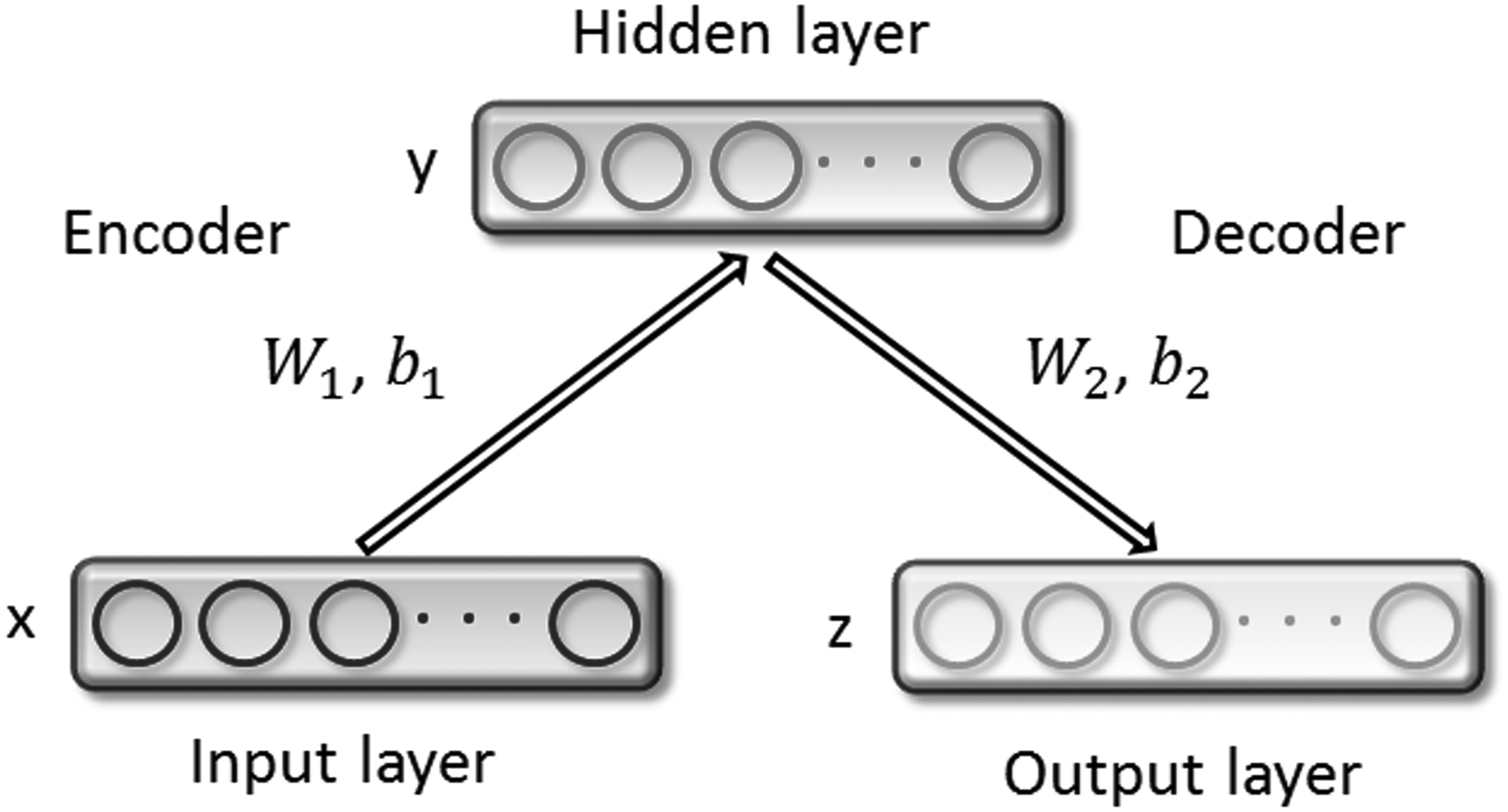
Stacked autoencoder (SAE) is a popular depth learning model, which uses autoencoders (AEs) as building blocks to create a deep neural network (Bengio et al., 2007). The AE is widely used for classification tasks and unsupervised feature learning, which tries to automatically generate the same features at the output layer as the input layer (Vincent et al., 2008; Rifai et al., 2011; Socher et al., 2011). It can be considered as a special neural network with one input layer, one hidden layer, and one output layer, as shown in Figure 1. Given a training sample X, the autocoder first encodes the input \documentclass{aastex}\usepackage{amsbsy}\usepackage{amsfonts}\usepackage{amssymb}\usepackage{bm}\usepackage{mathrsfs}\usepackage{pifont}\usepackage{stmaryrd}\usepackage{textcomp}\usepackage{portland, xspace}\usepackage{amsmath, amsxtra}\usepackage{upgreek}\pagestyle{empty}\DeclareMathSizes{10}{9}{7}{6}\begin{document} $${ \rm X} \in {{ \rm R}^{{d_0}}}$$ \end{document} into the hidden representation \documentclass{aastex}\usepackage{amsbsy}\usepackage{amsfonts}\usepackage{amssymb}\usepackage{bm}\usepackage{mathrsfs}\usepackage{pifont}\usepackage{stmaryrd}\usepackage{textcomp}\usepackage{portland, xspace}\usepackage{amsmath, amsxtra}\usepackage{upgreek}\pagestyle{empty}\DeclareMathSizes{10}{9}{7}{6}\begin{document} $${ \rm Y} \in {{ \rm R}^{{d_1}}}$$ \end{document} by the mapping \documentclass{aastex}\usepackage{amsbsy}\usepackage{amsfonts}\usepackage{amssymb}\usepackage{bm}\usepackage{mathrsfs}\usepackage{pifont}\usepackage{stmaryrd}\usepackage{textcomp}\usepackage{portland, xspace}\usepackage{amsmath, amsxtra}\usepackage{upgreek}\pagestyle{empty}\DeclareMathSizes{10}{9}{7}{6}\begin{document} $${{ \rm f}_c}$$ \end{document} : \documentclass{aastex}\usepackage{amsbsy}\usepackage{amsfonts}\usepackage{amssymb}\usepackage{bm}\usepackage{mathrsfs}\usepackage{pifont}\usepackage{stmaryrd}\usepackage{textcomp}\usepackage{portland, xspace}\usepackage{amsmath, amsxtra}\usepackage{upgreek}\pagestyle{empty}\DeclareMathSizes{10}{9}{7}{6}\begin{document} \begin{align*} Y = {f_c} \left( X \right) = {S_c} \left( {W_1^TX + {b_1}} \right) , \tag{2} \end{align*} \end{document}

FIG. 1.

Structure of autoencoder.

In the second step, the decoder maps the representation of the hidden layer Y to the output layer \documentclass{aastex}\usepackage{amsbsy}\usepackage{amsfonts}\usepackage{amssymb}\usepackage{bm}\usepackage{mathrsfs}\usepackage{pifont}\usepackage{stmaryrd}\usepackage{textcomp}\usepackage{portland, xspace}\usepackage{amsmath, amsxtra}\usepackage{upgreek}\pagestyle{empty}\DeclareMathSizes{10}{9}{7}{6}\begin{document} $$Z \in {R^{{d_0}}}$$ \end{document} by the mapping function \documentclass{aastex}\usepackage{amsbsy}\usepackage{amsfonts}\usepackage{amssymb}\usepackage{bm}\usepackage{mathrsfs}\usepackage{pifont}\usepackage{stmaryrd}\usepackage{textcomp}\usepackage{portland, xspace}\usepackage{amsmath, amsxtra}\usepackage{upgreek}\pagestyle{empty}\DeclareMathSizes{10}{9}{7}{6}\begin{document} $${{ \rm f}_d}$$ \end{document} . \documentclass{aastex}\usepackage{amsbsy}\usepackage{amsfonts}\usepackage{amssymb}\usepackage{bm}\usepackage{mathrsfs}\usepackage{pifont}\usepackage{stmaryrd}\usepackage{textcomp}\usepackage{portland, xspace}\usepackage{amsmath, amsxtra}\usepackage{upgreek}\pagestyle{empty}\DeclareMathSizes{10}{9}{7}{6}\begin{document} \begin{align*} Z = {f_d} \left( Y \right) = {S_d} \left( {W_2^TY + {b_2}} \right) , \tag{3} \end{align*} \end{document}

where \documentclass{aastex}\usepackage{amsbsy}\usepackage{amsfonts}\usepackage{amssymb}\usepackage{bm}\usepackage{mathrsfs}\usepackage{pifont}\usepackage{stmaryrd}\usepackage{textcomp}\usepackage{portland, xspace}\usepackage{amsmath, amsxtra}\usepackage{upgreek}\pagestyle{empty}\DeclareMathSizes{10}{9}{7}{6}\begin{document} $${{ \rm S}_d}$$ \end{document} is the activation function of the decoder, W₂ and b₂ is the parameter set with a weight matrix \documentclass{aastex}\usepackage{amsbsy}\usepackage{amsfonts}\usepackage{amssymb}\usepackage{bm}\usepackage{mathrsfs}\usepackage{pifont}\usepackage{stmaryrd}\usepackage{textcomp}\usepackage{portland, xspace}\usepackage{amsmath, amsxtra}\usepackage{upgreek}\pagestyle{empty}\DeclareMathSizes{10}{9}{7}{6}\begin{document} $${W_2} \in {R^{{d_0} \times {d_1}}}$$ \end{document} and a bias vector \documentclass{aastex}\usepackage{amsbsy}\usepackage{amsfonts}\usepackage{amssymb}\usepackage{bm}\usepackage{mathrsfs}\usepackage{pifont}\usepackage{stmaryrd}\usepackage{textcomp}\usepackage{portland, xspace}\usepackage{amsmath, amsxtra}\usepackage{upgreek}\pagestyle{empty}\DeclareMathSizes{10}{9}{7}{6}\begin{document} $${b_2} \in {r^{{d_0}}}$$ \end{document} . The parameters are learned by back-propagation through the minimizing the loss function \documentclass{aastex}\usepackage{amsbsy}\usepackage{amsfonts}\usepackage{amssymb}\usepackage{bm}\usepackage{mathrsfs}\usepackage{pifont}\usepackage{stmaryrd}\usepackage{textcomp}\usepackage{portland, xspace}\usepackage{amsmath, amsxtra}\usepackage{upgreek}\pagestyle{empty}\DeclareMathSizes{10}{9}{7}{6}\begin{document} $$\Theta \left( {X , Z} \right)$$ \end{document} in the formula 4. \documentclass{aastex}\usepackage{amsbsy}\usepackage{amsfonts}\usepackage{amssymb}\usepackage{bm}\usepackage{mathrsfs}\usepackage{pifont}\usepackage{stmaryrd}\usepackage{textcomp}\usepackage{portland, xspace}\usepackage{amsmath, amsxtra}\usepackage{upgreek}\pagestyle{empty}\DeclareMathSizes{10}{9}{7}{6}\begin{document} \begin{align*} \Theta \left( {X , Z} \right) = { \Theta _r} \left( {X , Z} \right) + 0.5 \tau \left( { \left\vert \vert {{W_1}} \right\vert \vert _2^2 + \left\vert \vert {{W_2}} \right\vert \vert _2^2} \right) , \tag{4} \end{align*} \end{document}

The combination of multiple AEs together constitutes the stacked AE, having the characteristics of deep learning. It can better learn the features of the input information and reduce the original data dimension (Salakhutdinov and Hinton, 2009). Figure 2 shows the structure of the stacked AE with h-level AEs, which are trained in the layer-wise and bottom-up manner. The input vector is received at the first level of the autocoder and sent to its hidden layer after training. The second layer of the AE receives data from the first layer and sent to its hidden layer after training. The raw data are transformed from layer to layer up to the top layer. The activation function is usually the sigmoid function or tanh function. After completing these unsupervised features training, the entire neural network can use the tagged data to fine-tune the training parameters. The hidden layer of the highest layer AE can be used as the feature of the original data extraction by the stacked AE and can be applied to classifiers. Stacked AE of deep learning can automatically take advantage of large amounts of unlabeled data and can learn higher level features from raw data and increase the performance of features. In this article, we set up a three-layer AE, and use the RF as the final classifier.

FIG. 2.

Structure of stacked autoencoders.

2.5. RF classifier

The RF proposed by Rodriguez and Kuncheva (2006) as a popular ensemble classifier has been widely used in various fields. Its main idea is to establish the ensemble classifiers that can balance both accuracy and diversity at the same time (Zhang and Zhang, 2010). In the execution of RF, the samples are first randomly divided into different subsets; then, each subset is rotated to increase diversity using the principal component analysis (PCA); finally, the transformed subsets are fed into different decision trees. The final result of the classification is generated by voting on these decision trees. The steps for RF are as follows:

Let M denote the sample set, \documentclass{aastex}\usepackage{amsbsy}\usepackage{amsfonts}\usepackage{amssymb}\usepackage{bm}\usepackage{mathrsfs}\usepackage{pifont}\usepackage{stmaryrd}\usepackage{textcomp}\usepackage{portland, xspace}\usepackage{amsmath, amsxtra}\usepackage{upgreek}\pagestyle{empty}\DeclareMathSizes{10}{9}{7}{6}\begin{document} $$X = { \left( {{x_1} , {x_2} , \ldots , {x_n}} \right) ^T}$$ \end{document} be an n × L matrix composed of n observation feature vector for each training sample, and \documentclass{aastex}\usepackage{amsbsy}\usepackage{amsfonts}\usepackage{amssymb}\usepackage{bm}\usepackage{mathrsfs}\usepackage{pifont}\usepackage{stmaryrd}\usepackage{textcomp}\usepackage{portland, xspace}\usepackage{amsmath, amsxtra}\usepackage{upgreek}\pagestyle{empty}\DeclareMathSizes{10}{9}{7}{6}\begin{document} $$Y = { \left( {{y_1} , {y_2} , \ldots , {y_n}} \right) ^T}$$ \end{document} denote the corresponding labels. Therefore, the training samples can be expressed as \documentclass{aastex}\usepackage{amsbsy}\usepackage{amsfonts}\usepackage{amssymb}\usepackage{bm}\usepackage{mathrsfs}\usepackage{pifont}\usepackage{stmaryrd}\usepackage{textcomp}\usepackage{portland, xspace}\usepackage{amsmath, amsxtra}\usepackage{upgreek}\pagestyle{empty}\DeclareMathSizes{10}{9}{7}{6}\begin{document} $$\left\{ {{x_i} , {y_i}} \right\} $$ \end{document} , in which \documentclass{aastex}\usepackage{amsbsy}\usepackage{amsfonts}\usepackage{amssymb}\usepackage{bm}\usepackage{mathrsfs}\usepackage{pifont}\usepackage{stmaryrd}\usepackage{textcomp}\usepackage{portland, xspace}\usepackage{amsmath, amsxtra}\usepackage{upgreek}\pagestyle{empty}\DeclareMathSizes{10}{9}{7}{6}\begin{document} $${x_i} = \left( {{x_{i1}} , {x_{i2}} , \ldots , {x_{iL}}} \right)$$ \end{document} be an L-dimensional feature vector. Suppose that the sample set is randomly divided into K subsets of the same size by an appropriate factor and transformed by PCA. Then, all the coefficients of the principal components are rearranged and stored to form a rotation matrix to change the original training set. In this case, P decision trees in the forest can be expressed as \documentclass{aastex}\usepackage{amsbsy}\usepackage{amsfonts}\usepackage{amssymb}\usepackage{bm}\usepackage{mathrsfs}\usepackage{pifont}\usepackage{stmaryrd}\usepackage{textcomp}\usepackage{portland, xspace}\usepackage{amsmath, amsxtra}\usepackage{upgreek}\pagestyle{empty}\DeclareMathSizes{10}{9}{7}{6}\begin{document} $${R_1} , {R_2} , \ldots , {R_P}$$ \end{document} , respectively. The preprocessing steps of the training set for a single classifier \documentclass{aastex}\usepackage{amsbsy}\usepackage{amsfonts}\usepackage{amssymb}\usepackage{bm}\usepackage{mathrsfs}\usepackage{pifont}\usepackage{stmaryrd}\usepackage{textcomp}\usepackage{portland, xspace}\usepackage{amsmath, amsxtra}\usepackage{upgreek}\pagestyle{empty}\DeclareMathSizes{10}{9}{7}{6}\begin{document} $${{ \rm R}_i}$$ \end{document} are shown below:

(1) The sample set M is randomly divided into K (a factor of n) disjoint subsets, and each subset containing the number of features is \documentclass{aastex}\usepackage{amsbsy}\usepackage{amsfonts}\usepackage{amssymb}\usepackage{bm}\usepackage{mathrsfs}\usepackage{pifont}\usepackage{stmaryrd}\usepackage{textcomp}\usepackage{portland, xspace}\usepackage{amsmath, amsxtra}\usepackage{upgreek}\pagestyle{empty}\DeclareMathSizes{10}{9}{7}{6}\begin{document} $${ \raise0.7ex \hbox{\$ n \$} \mathord{ \left/ { \vphantom {n k}} \right. \kern - \nulldelimiterspace} \lower0.7ex \hbox{\$ k \$}}$$ \end{document} .

(2) Select the corresponding column of the feature in the subset \documentclass{aastex}\usepackage{amsbsy}\usepackage{amsfonts}\usepackage{amssymb}\usepackage{bm}\usepackage{mathrsfs}\usepackage{pifont}\usepackage{stmaryrd}\usepackage{textcomp}\usepackage{portland, xspace}\usepackage{amsmath, amsxtra}\usepackage{upgreek}\pagestyle{empty}\DeclareMathSizes{10}{9}{7}{6}\begin{document} $${M_{i , j}}$$ \end{document} to form a new matrix \documentclass{aastex}\usepackage{amsbsy}\usepackage{amsfonts}\usepackage{amssymb}\usepackage{bm}\usepackage{mathrsfs}\usepackage{pifont}\usepackage{stmaryrd}\usepackage{textcomp}\usepackage{portland, xspace}\usepackage{amsmath, amsxtra}\usepackage{upgreek}\pagestyle{empty}\DeclareMathSizes{10}{9}{7}{6}\begin{document} $${X_{i , j}}$$ \end{document} from the training data set X. A new training set \documentclass{aastex}\usepackage{amsbsy}\usepackage{amsfonts}\usepackage{amssymb}\usepackage{bm}\usepackage{mathrsfs}\usepackage{pifont}\usepackage{stmaryrd}\usepackage{textcomp}\usepackage{portland, xspace}\usepackage{amsmath, amsxtra}\usepackage{upgreek}\pagestyle{empty}\DeclareMathSizes{10}{9}{7}{6}\begin{document} $${X ^{\prime} _{i , j}}$$ \end{document} is extracted from \documentclass{aastex}\usepackage{amsbsy}\usepackage{amsfonts}\usepackage{amssymb}\usepackage{bm}\usepackage{mathrsfs}\usepackage{pifont}\usepackage{stmaryrd}\usepackage{textcomp}\usepackage{portland, xspace}\usepackage{amsmath, amsxtra}\usepackage{upgreek}\pagestyle{empty}\DeclareMathSizes{10}{9}{7}{6}\begin{document} $${X_{i , j}}$$ \end{document} randomly with 75% of the data set using bootstrap algorithm. Loop K times in this way, so that each subset is converted.

(3) Matrix \documentclass{aastex}\usepackage{amsbsy}\usepackage{amsfonts}\usepackage{amssymb}\usepackage{bm}\usepackage{mathrsfs}\usepackage{pifont}\usepackage{stmaryrd}\usepackage{textcomp}\usepackage{portland, xspace}\usepackage{amsmath, amsxtra}\usepackage{upgreek}\pagestyle{empty}\DeclareMathSizes{10}{9}{7}{6}\begin{document} $${X ^{\prime} _{i , j}}$$ \end{document} is used as the feature transformed by PCA technique for producing the coefficient matrix \documentclass{aastex}\usepackage{amsbsy}\usepackage{amsfonts}\usepackage{amssymb}\usepackage{bm}\usepackage{mathrsfs}\usepackage{pifont}\usepackage{stmaryrd}\usepackage{textcomp}\usepackage{portland, xspace}\usepackage{amsmath, amsxtra}\usepackage{upgreek}\pagestyle{empty}\DeclareMathSizes{10}{9}{7}{6}\begin{document} $${S_{i , j}}$$ \end{document} , with jth column coefficient as the characteristic component jth.

(4) A sparse rotation matrix \documentclass{aastex}\usepackage{amsbsy}\usepackage{amsfonts}\usepackage{amssymb}\usepackage{bm}\usepackage{mathrsfs}\usepackage{pifont}\usepackage{stmaryrd}\usepackage{textcomp}\usepackage{portland, xspace}\usepackage{amsmath, amsxtra}\usepackage{upgreek}\pagestyle{empty}\DeclareMathSizes{10}{9}{7}{6}\begin{document} $${{ \rm G}_i}$$ \end{document} is constructed, and its coefficients obtained from the matrix \documentclass{aastex}\usepackage{amsbsy}\usepackage{amsfonts}\usepackage{amssymb}\usepackage{bm}\usepackage{mathrsfs}\usepackage{pifont}\usepackage{stmaryrd}\usepackage{textcomp}\usepackage{portland, xspace}\usepackage{amsmath, amsxtra}\usepackage{upgreek}\pagestyle{empty}\DeclareMathSizes{10}{9}{7}{6}\begin{document} $${S_{i , j}}$$ \end{document} expressed as follows:

\documentclass{aastex}\usepackage{amsbsy}\usepackage{amsfonts}\usepackage{amssymb}\usepackage{bm}\usepackage{mathrsfs}\usepackage{pifont}\usepackage{stmaryrd}\usepackage{textcomp}\usepackage{portland, xspace}\usepackage{amsmath, amsxtra}\usepackage{upgreek}\pagestyle{empty}\DeclareMathSizes{10}{9}{7}{6}\begin{document} \begin{align*} {G_i} = \left[{\begin{matrix} { \varkappa_{i , 1}^{ \left( 1 \right) } , \ldots , \varkappa_{i , 1}^{ \left( {{C_1}} \right) }} & 0 & \cdots & 0 \\ 0 & { \varkappa_{i , 2}^{ \left( 1 \right) } , \cdots , \varkappa_{i , 2}^{ \left( {{C_2}} \right) }} & \cdots & 0 \\ \vdots & \vdots & \ddots & \vdots \\ 0 & 0 & \cdots & { \varkappa_{i , k}^{ \left( 1 \right) } , \ldots , \varkappa_{i , k}^{ \left( {{C_k}} \right) }}\end{matrix}} \right]. \tag{4} \end{align*} \end{document}

The prediction period, provided the test sample x, generated by the classifier \documentclass{aastex}\usepackage{amsbsy}\usepackage{amsfonts}\usepackage{amssymb}\usepackage{bm}\usepackage{mathrsfs}\usepackage{pifont}\usepackage{stmaryrd}\usepackage{textcomp}\usepackage{portland, xspace}\usepackage{amsmath, amsxtra}\usepackage{upgreek}\pagestyle{empty}\DeclareMathSizes{10}{9}{7}{6}\begin{document} $${{ \rm R}_i}$$ \end{document} of \documentclass{aastex}\usepackage{amsbsy}\usepackage{amsfonts}\usepackage{amssymb}\usepackage{bm}\usepackage{mathrsfs}\usepackage{pifont}\usepackage{stmaryrd}\usepackage{textcomp}\usepackage{portland, xspace}\usepackage{amsmath, amsxtra}\usepackage{upgreek}\pagestyle{empty}\DeclareMathSizes{10}{9}{7}{6}\begin{document} $${d_{i , j}} \left( {XG_i^ \varkappa } \right)$$ \end{document} to determine x belongs to class \documentclass{aastex}\usepackage{amsbsy}\usepackage{amsfonts}\usepackage{amssymb}\usepackage{bm}\usepackage{mathrsfs}\usepackage{pifont}\usepackage{stmaryrd}\usepackage{textcomp}\usepackage{portland, xspace}\usepackage{amsmath, amsxtra}\usepackage{upgreek}\pagestyle{empty}\DeclareMathSizes{10}{9}{7}{6}\begin{document} $${{ \rm y}_i}$$ \end{document} . And then the class of confidence is calculated by means of the average combination, and the formula is as follows: \documentclass{aastex}\usepackage{amsbsy}\usepackage{amsfonts}\usepackage{amssymb}\usepackage{bm}\usepackage{mathrsfs}\usepackage{pifont}\usepackage{stmaryrd}\usepackage{textcomp}\usepackage{portland, xspace}\usepackage{amsmath, amsxtra}\usepackage{upgreek}\pagestyle{empty}\DeclareMathSizes{10}{9}{7}{6}\begin{document} \begin{align*} { \theta _j } \left( x \right) = \frac { 1 } { P } \mathop \sum \limits_ { i = 1 } ^P { d_ { i , j } } \left( { XG_i^ \varkappa } \right). \tag { 5 } \end{align*} \end{document}

Therefore, the test sample x is easily assigned to the classes with the greatest possibility. In this experiment, the parameters of the RF are optimized by the grid search method, and finally set K to 52 and L to 5. The flow chart of the proposed method is shown in Figure 3.

FIG. 3.

The flow chart of the proposed method.

3. Results and Discussion

3.1. Evaluation criteria

Evaluation criteria are particularly important for measuring methods. The advantages and disadvantages of this method can be objectively reflected by comparing with other methods under the unified evaluation criteria. The evaluation criteria used in this article include accuracy (Accu.), sensitivity (Sen.), precision (Prec.), and Matthews correlation coefficient (MCC). They are calculated as follows: \documentclass{aastex}\usepackage{amsbsy}\usepackage{amsfonts}\usepackage{amssymb}\usepackage{bm}\usepackage{mathrsfs}\usepackage{pifont}\usepackage{stmaryrd}\usepackage{textcomp}\usepackage{portland, xspace}\usepackage{amsmath, amsxtra}\usepackage{upgreek}\pagestyle{empty}\DeclareMathSizes{10}{9}{7}{6}\begin{document} \begin{align*} Accu. = { \frac { TP + TN } { TP + TN + FP + FN } } , \tag { 6 } \end{align*} \end{document} \documentclass{aastex}\usepackage{amsbsy}\usepackage{amsfonts}\usepackage{amssymb}\usepackage{bm}\usepackage{mathrsfs}\usepackage{pifont}\usepackage{stmaryrd}\usepackage{textcomp}\usepackage{portland, xspace}\usepackage{amsmath, amsxtra}\usepackage{upgreek}\pagestyle{empty}\DeclareMathSizes{10}{9}{7}{6}\begin{document} \begin{align*} Sen. = { \frac { TP } { TP + FN } } , \tag { 7 } \end{align*} \end{document} \documentclass{aastex}\usepackage{amsbsy}\usepackage{amsfonts}\usepackage{amssymb}\usepackage{bm}\usepackage{mathrsfs}\usepackage{pifont}\usepackage{stmaryrd}\usepackage{textcomp}\usepackage{portland, xspace}\usepackage{amsmath, amsxtra}\usepackage{upgreek}\pagestyle{empty}\DeclareMathSizes{10}{9}{7}{6}\begin{document} \begin{align*} { \rm Prec } . = { \frac { TP } { { \rm TP } + { \rm FP } } } , \tag { 8 } \end{align*} \end{document} \documentclass{aastex}\usepackage{amsbsy}\usepackage{amsfonts}\usepackage{amssymb}\usepackage{bm}\usepackage{mathrsfs}\usepackage{pifont}\usepackage{stmaryrd}\usepackage{textcomp}\usepackage{portland, xspace}\usepackage{amsmath, amsxtra}\usepackage{upgreek}\pagestyle{empty}\DeclareMathSizes{10}{9}{7}{6}\begin{document} \begin{align*} MCC = { \frac { TP \times TN - FP \times FN } { \sqrt { \left( { TP + FP } \right) \left( { TP + FN } \right) \left( { TN + FP } \right) \left( { TN + FN } \right) } } } , \tag { 9 } \end{align*} \end{document}

where TP (true positive) denotes the number of positive samples correctly identified; FP (false positive) denotes the number of positive samples incorrectly identified; TN (true negative) denotes the number of negative samples correctly identified; FN (false negative) denotes the number of negative samples incorrectly identified. The receiver operating characteristic (ROC) curve (Zweig and Campbell, 1993) is introduced to visually display the performance of classifier.

3.2. Assessment of prediction ability

In this article, we use fivefold cross-validation to assess the predictive ability of our model in the gold standard data sets involving enzymes, ion channels, GPCRs, and nuclear receptors. Cross-validation can not only prevent overfitting but also can test the stability of the model. Its implementation steps are as follows: first, all the samples are randomly divided into five disjoint subsets of equal number; then, each time one different subset is used as test set, the remaining four are used as training set, so that the formation of five models; finally, the five models are used to predict the classification, and the average value of them is the final result.

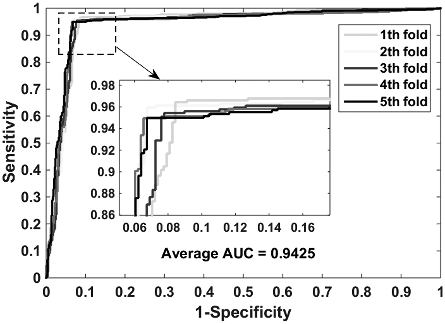
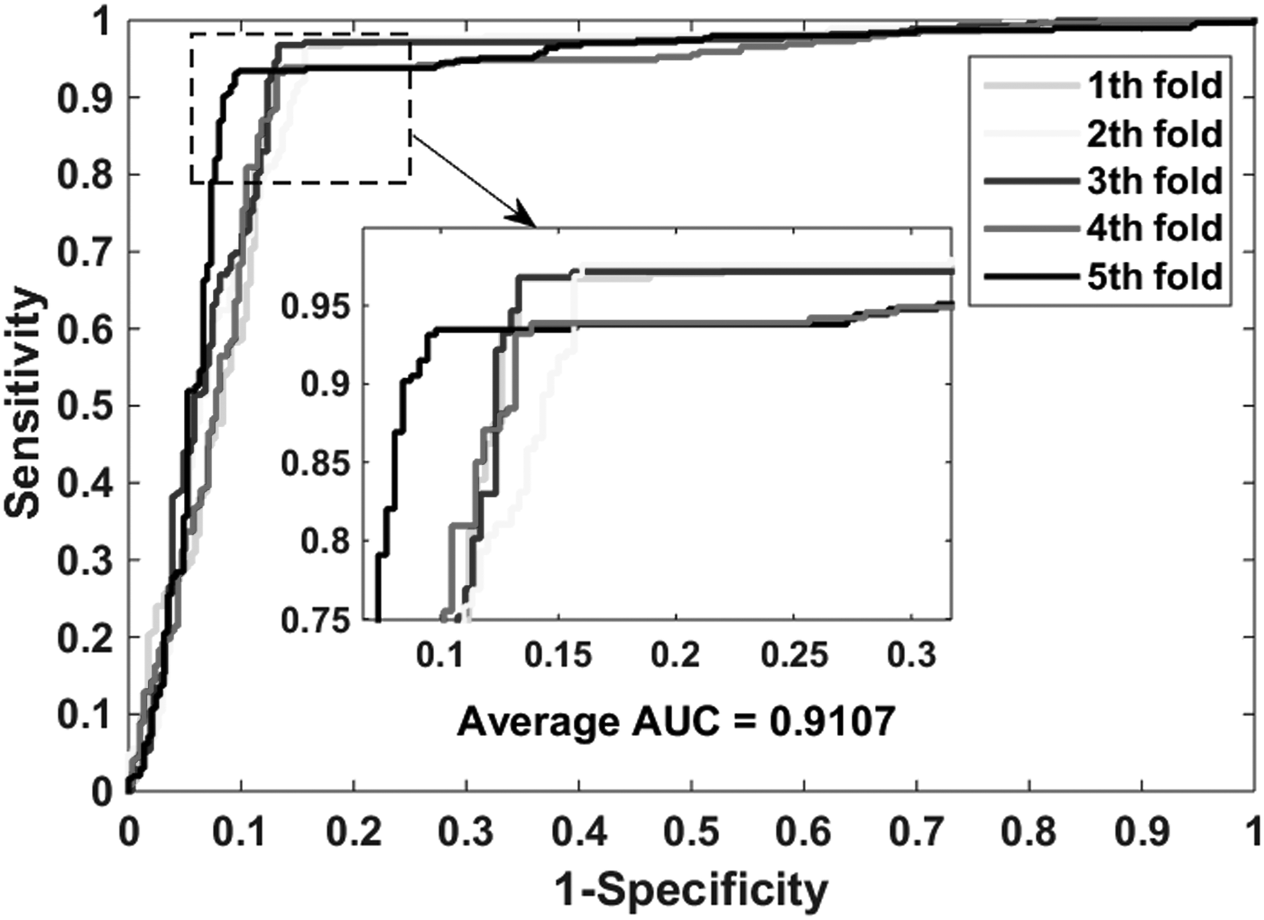
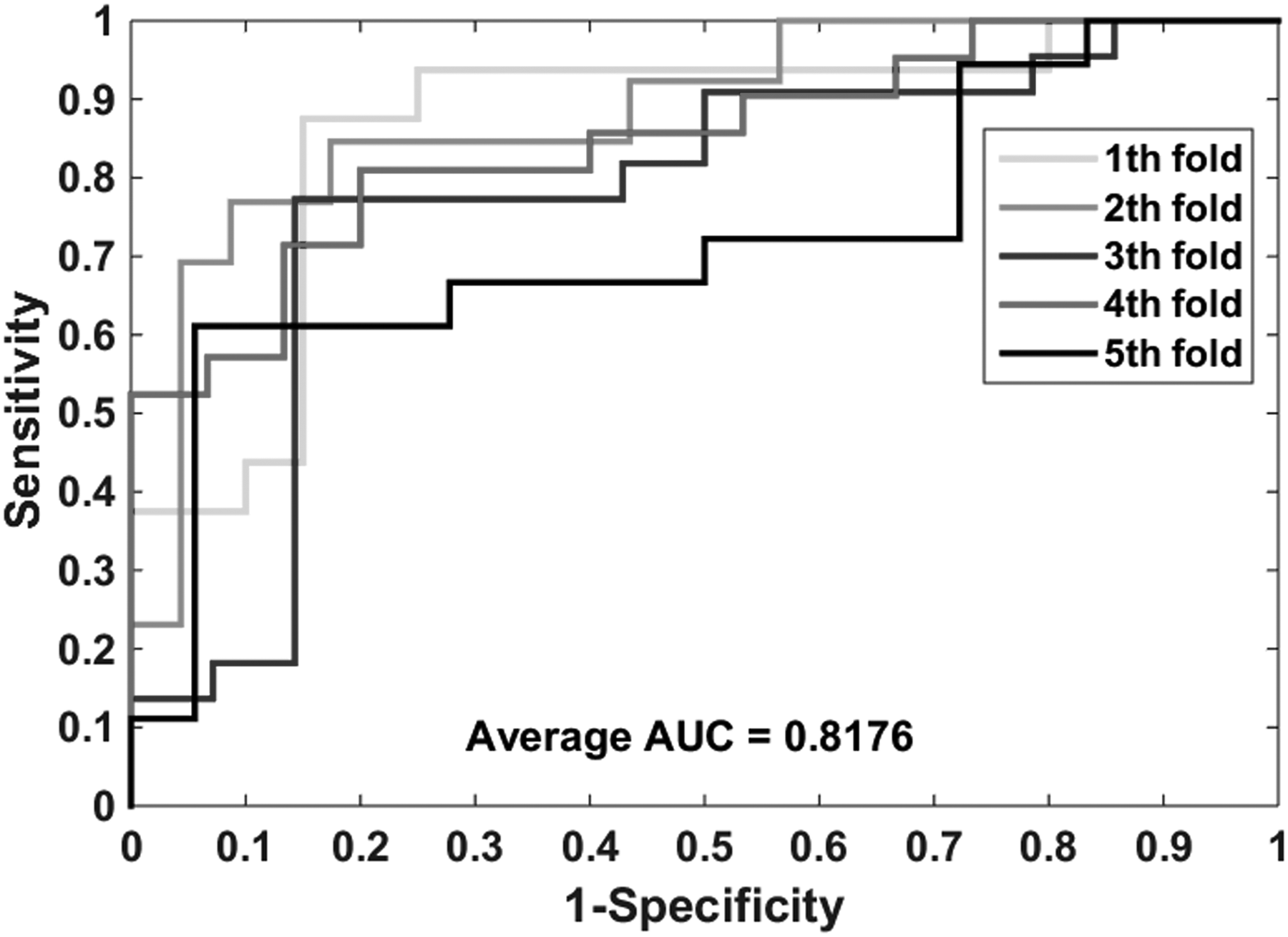
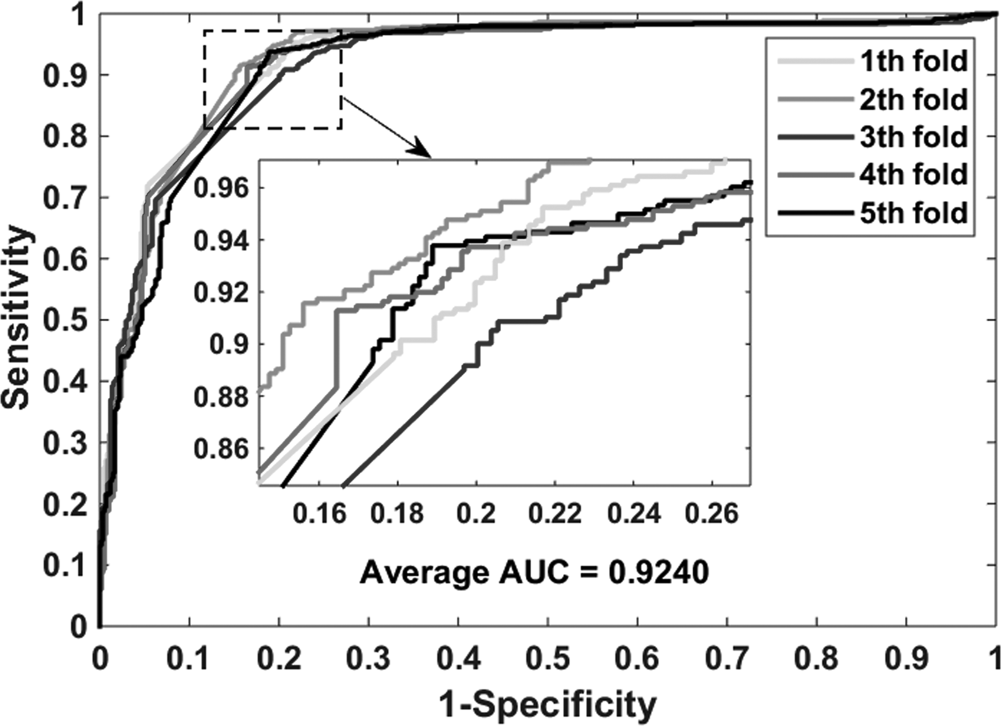
The proposed model performs well in the gold standard data sets: enzymes, ion channels, GPCRs, and nuclear receptors. Table 2 lists the experimental results on the enzyme data set, it yielded an accuracy of 0.9414, sensitivity of 0.9555, precision of 0.9293, MCC of 0.8832, and AUC (area under receiver operating characteristic curve) of 0.9425. And their standard deviations are 0.0030, 0.0064, 0.0067, 0.0058, and 0.0022, respectively. The highest accuracy of the five models reached 0.9462, and the lowest also reached 0.9385. Table 3 shows the performance of our model implementation in the icon channel data set. The accuracy, sensitivity, precision, MCC, and AUC of cross-validation are 0.9116, 0.9569, 0.8778, 0.8271, and 0.9107, respectively. The standard deviations for these criterion values are 0.0086, 0.0188, 0.0219, 0.0162, and 0.0074, respectively. Table 4 lists the results when the GPCR data set is used to predict drug–target interactions. The average accuracy, sensitivity, precision, MCC, and AUC are 0.8669, 0.8164, 0.9102, 0.7396, and 0.8743, respectively. The standard deviations for these criterion values are 0.0446, 0.0651, 0.0380, 0.0837, and 0.0417, respectively. The highest accuracy of the five models reached 0.9331. Table 5 summarizes the statistical results of the cross-validation of nuclear receptor data set. We achieved an accuracy of 0.8056, sensitivity of 0.7627, precision of 0.8410, MCC of 0.6188, and AUC of 0.8176. Their standard deviations are 0.0439, 0.1284, 0.0688, 0.0712, and 0.0676, respectively. Figures 4 –7 show the ROC curves obtained on the enzyme, ion channel, GPCR, and nuclear receptor data sets by the proposed method.

FIG. 4.

The ROC curves were generated on the enzyme data set by using the proposed method. ROC, receiver operating characteristic.

FIG. 5.

The ROC curves were generated on the icon channel data set by using the proposed method.

FIG. 6.

The ROC curves were generated on the GPCR data set by using the proposed method.

FIG. 7.

The ROC curves were generated on the nuclear receptor data set by using the proposed method.

Table 2.

The Fivefold Cross-Validation Results Were Generated on the Enzyme Data Set by Using the Proposed Method

Test set	Accu. (%)	Sen. (%)	Prec. (%)	MCC (%)	AUC (%)
1	93.93	96.43	91.91	87.97	94.50
2	94.62	95.95	93.59	89.25	94.21
3	93.85	95.43	92.61	87.73	94.03
4	94.19	94.95	93.32	88.39	94.05
5	94.11	94.99	93.22	88.24	94.46
Average	94.14 ± 0.30	95.55 ± 0.64	92.93 ± 0.67	88.32 ± 0.58	94.25 ± 0.22

AUC, area under receiver operating characteristic curve; Accu., accuracy; Sen., sensitivity; Prec., precision; MCC, Matthews correlation coefficient.

Table 3.

The Fivefold Cross-Validation Results Were Generated on the Icon Channel Data Set by Using the Proposed Method

Test set	Accu. (%)	Sen. (%)	Prec. (%)	MCC (%)	AUC (%)
1	91.86	96.71	88.55	84.05	90.91
2	90.51	97.59	85.24	81.89	91.28
3	91.53	96.81	86.94	83.59	91.62
4	90.00	93.88	87.07	80.25	89.86
5	91.89	93.46	91.08	83.78	91.69
Average	91.16 ± 0.86	95.69 ± 1.88	87.78 ± 2.19	82.71 ± 1.62	91.07 ± 0.74

Table 4.

The Fivefold Cross-Validation Results Were Generated on the GPCR Data Set by Using the Proposed Method

Test set	Accu. (%)	Sen. (%)	Prec. (%)	MCC (%)	AUC (%)
1	86.61	82.68	89.74	73.46	86.56
2	93.31	91.13	94.96	86.66	92.97
3	83.46	79.51	85.09	66.93	83.84
4	81.89	73.05	92.79	66.09	83.39
5	88.19	81.82	92.52	76.68	90.40
Average	86.69 ± 4.46	81.64 ± 6.51	91.02 ± 3.80	73.96 ± 8.37	87.43 ± 4.17

Table 5.

The Fivefold Cross-Validation Results Were Generated on the Nuclear Receptor Data Set by Using the Proposed Method

Test set	Accu. (%)	Sen. (%)	Prec. (%)	MCC (%)	AUC (%)
1	86.11	87.50	82.35	72.16	86.25
2	83.33	84.62	73.33	65.49	88.29
3	77.78	72.73	88.89	56.98	77.27
4	80.56	80.95	85.00	60.47	84.76
5	75.00	55.56	90.91	54.27	72.22
Average	80.56 ± 4.39	76.27 ± 12.84	84.10 ± 6.88	61.88 ± 7.12	81.76 ± 6.76

3.3. Comparison between discrete cosine transform descriptor and SAE descriptor

To verify the ability of the extracted feature to represent the raw data, we compare SAE descriptor with the discrete cosine transform (DCT) descriptor on the enzyme data set. DCT algorithm has the advantage of losing only a small amount of information during data conversion, so it is often used as a feature extraction method. It is calculated as follows: \documentclass{aastex}\usepackage{amsbsy}\usepackage{amsfonts}\usepackage{amssymb}\usepackage{bm}\usepackage{mathrsfs}\usepackage{pifont}\usepackage{stmaryrd}\usepackage{textcomp}\usepackage{portland, xspace}\usepackage{amsmath, amsxtra}\usepackage{upgreek}\pagestyle{empty}\DeclareMathSizes{10}{9}{7}{6}\begin{document} \begin{align*} DCT \left( { i , j } \right) = \theta \left( i \right) \theta \left( j \right) \mathop \sum \limits_ { x = 0 } ^ { u - 1 } \ \mathop \sum \limits_ { y = 0 } ^ { v - 1 } f \left( { x , y } \right) \cos { \frac { \pi \left( { 2x + 1 } \right) i } { 2u } } \cos { \frac { \pi \left( { 2y + 1 } \right) j } { 2v } } \ 0 \le i \le u - 1 , \ 0 \le j \le v - 1 , \tag { 10 } \end{align*} \end{document}

Table 6 summarizes the results of cross-validation on the enzyme data set generated by using the DCT descriptor. The yielded average results of accuracy, sensitivity, precision, and MCC are 0.8865, 0.8965, 0.8791, and 0.7734, respectively. However, the accuracy, sensitivity, precision, and MCC of the cross-validation generated by the SAE descriptor are 0.9414, 0.9555, 0.9293, and 0.8832, which are 5.49%, 5.90%, 5.02%, and 10.98% higher than the DCT descriptor, respectively. The experimental results show that the features extracted by the SAE algorithm contain more information about the raw data than those extracted by the DCT algorithm.

Table 6.

The Fivefold Cross-Validation Results Were Generated on the Enzyme Data Set by Using the Discrete Cosine Transform Descriptors

Test set	Accu. (%)	Sen. (%)	Prec. (%)	MCC (%)
1	88.55	90.43	87.15	77.15
2	88.03	89.12	87.33	76.08
3	89.23	90.28	88.80	78.46
4	89.23	91.40	87.12	78.56
5	88.23	87.03	89.16	76.47
Average	88.65 ± 0.56	89.65 ± 1.68	87.91 ± 0.98	77.34 ± 1.13
Our method	94.14 ± 0.30	95.55 ± 0.64	92.93 ± 0.67	88.32 ± 0.58

3.4. Comparison between RF classifier and support vector machine classifier

Support vector machine (SVM) is a supervised learning algorithm, which has outstanding performance on regression tasks and two-class classification problems (Smola and Scholkopf, 2004; Cao et al., 2010, 2011). In this section, we use the same features to compare the proposed classifier with the state-of-the-art SVM classifier. After the parameters of the SVM are optimized by the grid search method, the parameter c is set to 20, g is set to 800. The results of the comparison between them on the enzyme data set are summarized in Table 7. Our method has achieved good results on all evaluation criteria, including accuracy, sensitivity, precision, MCC, and AUC. They increased by 7.59%, 3.27%, 10.11%, 14.37%, and 1.85%, respectively. While the standard deviations decreased by 0.82%, 0.28%, 0.80%, 1.58%, and 0.34%, respectively. Figure 8 shows the ROC curves obtained on the enzyme data set by using the SVM classifier.

FIG. 8.

The ROC curves were generated on the enzyme data set by using the SVM classifier. SVM, support vector machine.

Table 7.

Comparison of Cross-Validation Results Between the Rotation Forest Classifier and the Support Vector Machine Classifier on the Enzyme Data Set

Test set	Accu. (%)	Sen. (%)	Prec. (%)	MCC (%)	AUC (%)
1	86.41	93.21	82.19	73.47	92.85
2	87.61	92.07	84.78	75.47	93.12
3	84.70	91.37	80.84	69.97	92.00
4	86.92	91.46	83.47	74.21	92.25
5	87.12	93.26	82.82	74.85	91.80
Average	86.55 ± 1.12	92.28 ± 0.92	82.82 ± 1.47	73.95 ± 2.16	92.40 ± 0.56
Our method	94.14 ± 0.30	95.55 ± 0.64	92.93 ± 0.67	88.32 ± 0.58	94.25 ± 0.22

3.5. Comparison with state-of-the-art methods

To test the robustness and reliability of the proposed method, we compared it with state-of-the-art methods on the gold standard data sets. We collected the AUC values generated by the four methods on the enzyme, ion channel, GPCR, and nuclear receptor data sets. As shown in Table 8, our method performs best on the enzyme, ion channel, and GPCR data sets with AUC values of 0.9425, 0.9107, and 0.8743, respectively. On the nuclear receptor data set, the highest value obtained by the NetCBP method is 0.856, but our method also achieved 0.8176 results, which is only 3.84% lower than it, also reached the average level. The results of the comparison show that the stacked AE combined with the RF classifier can improve the prediction ability on the gold standard data sets.

Table 8.

State-of-the-Art Methods and Our Method Obtained the AUC Values on the Gold Standard Data Sets

Method	Enzymes	Icon channels	GPCRs	Nuclear receptors
KBMF2K (Gonen, 2012)	0.832	0.799	0.857	0.824
DBSI (Cheng et al., 2012)	0.8075	0.8029	0.8022	0.7578
NetCBP (Chen and Zhang, 2013)	0.8251	0.8034	0.8235	0.8394
Yamanishi (Yamanishi et al., 2010)	0.821	0.692	0.811	0.814
WNN-GIP (Laarhoven and Marchiori, 2013)	0.861	0.775	0.872	0.839
SIMCOMP (Öztürk et al., 2016)	0.863	0.776	0.867	0.856
NLCS (Öztürk et al., 2016)	0.837	0.753	0.853	0.815
Our method	0.9425	0.9107	0.8743	0.8176

Boldface represents the best result in this data set.

4. Conclusion

In this article, based on the idea that the relationship between drugs and targets is largely influenced by the chemical structure of the drug and the sequence information of the protein, we propose a novel computational method to infer potential unknown drug–target interactions on a genome-wide scale by integrating protein amino acid sequence and drug molecular structure. To extract more representative features, we use deep learning technology to learn the protein sequence that is converted into the matrix containing biological evolutionary information. And then combine with the molecular fingerprint information to form the feature descriptor sent to the RF for classification. The proposed method is applied to four classes of target proteins, including enzymes, ion channels, GPCRs, and nuclear receptors. To evaluate the performance of our method, we experimented with different feature extraction methods and classifiers, and compared with other methods. Excellent experimental results show that our method has a prominent ability in mining the hidden interactions between drugs and targets. We have reasons to believe that the proposed method will play an important role in promoting the research and development of drugs. In future work, we plan to integrate more biology knowledge, using more advanced machine learning methods to improve the ability to predict.

Footnotes

Acknowledgments

This work is supported, in part, by the Fundamental Research Funds for the Central Universities, under Grants 2017BSCXB43 and, in part, by the Research and Innovation Project for College Graduates of Jiangsu Province, under Grant KYCX17_1559. The authors thank all anonymous reviewers for their constructive advices.

Author Disclosure Statement

No competing financial interests exist.

References

Altschul

S.F.

, Madden

T.L.

, Schaffer

A.A.

, et al. 1997. Gapped BLAST and PSI-BLAST: A new generation of protein database search programs. Nucleic Acids Res. 25, 3389–3402.

Bengio

, Lamblin

, Popovici

, et al. 2007. Greedy layer-wise training of deep networks. Adv. Neural Inf. Process. Syst. 19, 153.

Cao

D.-S.

, Liang

Y.-Z.

, Xu

Q.-S.

, et al. 2011. Exploring nonlinear relationships in chemical data using kernel-based methods. Chemometr. Intell. Lab. Syst., 107, 106–115.

Cao

D.-S.

, Xu

Q.-S.

, Liang

Y.-Z.

, et al. 2010. Prediction of aqueous solubility of druglike organic compounds using partial least squares, back-propagation network and support vector machine. J. Chemometrics, 24, 584–595.

Chen

, and Zhang

2013. A semi-supervised method for drug-target interaction prediction with consistency in networks. PLoS One, 8, e62975.

Chen

X.-W.

, and Jeong

J.C.

2009. Sequence-based prediction of protein interaction sites with an integrative method. Bioinformatics, 25, 585–591.

Chen

, Liu

M.X.

, and Yan

G.Y.

2012. Drug-target interaction prediction by random walk on the heterogeneous network. Mol. Biosyst., 8, 1970–1978.

Chen

, Yan

C.C.

, Zhang

, et al. 2016. Drug–target interaction prediction: Databases, web servers and computational models. Brief. Bioinf., 17, 696–712.

Cheng

, Liu

, Jiang

, et al. 2012. Prediction of drug-target interactions and drug repositioning via network-based inference. PLoS Comput. Biol. 8, e1002503.

10.

Dickson

, and Gagnon

J.P.

2004. Key factors in the rising cost of new drug discovery and development. Nat. Rev. Drug Discov., 3, 417–429.

11.

Gao

Z.G.

, Wang

, Xia

S.X.

, et al. 2016. Ens-PPI: A novel ensemble classifier for predicting the interactions of proteins using autocovariance transformation from PSSM. Biomed Res. Int., 8.

12.

Gonen

2012. Predicting drug-target interactions from chemical and genomic kernels using Bayesian matrix factorization. Bioinformatics, 28, 2304–2310.

13.

Gribskov

, McLachlan

A.D.

, and Eisenberg

1987. Profile analysis: Detection of distantly related proteins. Proc. Natl Acad. Sci. U. S. A., 84, 4355–4358.

14.

Gunther

, Kuhn

, Dunkel

, et al. 2008. SuperTarget and Matador: Resources for exploring drug-target relationships. Nucl. Acids Res., 36, D919–D922.

15.

Hopkins

A.L.

2008. Network pharmacology: The next paradigm in drug discovery. Nat. Chem. Biol., 4, 682–690.

16.

Iskar

, Zeller

, Zhao

X.-M.

, et al. 2012. Drug discovery in the age of systems biology: The rise of computational approaches for data integration. Curr. Opin. Biotechnol., 23, 609–616.

17.

Jones

D.T.

1999. Protein secondary structure prediction based on position-specific scoring matrices. J. Mol. Biol., 292, 195–202.

18.

Jones

D.T.

, and Ward

J.J.

2003. Prediction of disordered regions in proteins from position specific score matrices. Proteins, 53, 573–578.

19.

Kanehisa

, Goto

, Hattori

, et al. 2006. From genomics to chemical genomics: New developments in KEGG. Nucl. Acids Res., 34, D354–D357.

20.

Keiser

M.J.

, Setola

, Irwin

J.J.

, et al. 2009. Predicting new molecular targets for known drugs. Nature, 462, 175–181.

21.

Kola

, and Landis

2004. Can the pharmaceutical industry reduce attrition rates?. Nat. Rev. Drug Discov., 3, 711–715.

22.

Laarhoven

T.V.

, and Marchiori

2013. Predicting drug-target interactions for new drug compounds using a weighted nearest neighbor profile. PLos One, 8, e66952.

23.

Öztürk

, Ozkirimli

, and Özgür

2016. A comparative study of SMILES-based compound similarity functions for drug-target interaction prediction. BMC Bioinformatics, 17, 1–11.

24.

Paul

S.M.

, Mytelka

D.S.

, Dunwiddie

C.T.

, et al. 2010. How to improve R&D productivity: The pharmaceutical industry's grand challenge. Nat. Rev. Drug Discov., 9, 203–214.

25.

Rifai

, Vincent

, Muller

, et al. 2011. Contractive auto-encoders: Explicit invariance during feature extraction. In Proceedings of the 28th International Conference on Machine Learning (ICML-11), 833–840. Washington, DC.

26.

Rodriguez

J.J.

, and Kuncheva

L.I.

2006. Rotation forest: A new classifier ensemble method. IEEE Trans. Pattern Anal. Mach. Intell., 28, 1619–1630.

27.

Salakhutdinov

, and Hinton

2009. Semantic hashing. Int. J. Approx. Reason., 50, 969–978.

28.

Schomburg

, Chang

, Ebeling

, et al. 2004. BRENDA, the enzyme database: Updates and major new developments. Nucl. Acids Res., 32, D431–D433.

29.

Shen

, Cheng

F.X.

, Xu

, et al. 2010. Estimation of ADME properties with substructure pattern recognition. J. Chem. Inf. Model., 50, 1034–1041.

30.

Smola

A.J.

, and Scholkopf

2004. A tutorial on support vector regression. Stat. Comput., 14, 199–222.

31.

Socher

, Pennington

, Huang

E.H.

, et al. 2011. Semi-supervised recursive autoencoders for predicting sentiment distributions. In Proceedings of the Conference on Empirical Methods in Natural Language Processing. Association for Computational Linguistics, 151–161. University of Edinburgh, UK.

32.

Sun

, Bao

, You

, et al. 2016. Modeling of signaling crosstalk-mediated drug resistance and its implications on drug combination. Oncotarget, 7, 63995–64006.

33.

Vincent

, Larochelle

, Bengio

, et al. 2008. Extracting and composing robust features with denoising autoencoders. In Proceedings of the 25th International Conference on Machine Learning. ACM, 1096–1103. Helsinki, Finland.

34.

Wang

, You

Z.H.

, Chen

, et al. 2017a. An ensemble approach for large-scale identification of protein-protein interactions using the alignments of multiple sequences. Oncotarget, 8, 5149.

35.

Wang

, You

Z.-H.

, Xia

S.-X.

, et al. 2017b. An improved efficient rotation forest algorithm to predict the interactions among proteins. Soft Comput. 17, 1–9.

36.

Wang

, You

Z.-H.

, Xia

S.-X.

, et al. 2017c. Advancing the prediction accuracy of protein-protein interactions by utilizing evolutionary information from position-specific scoring matrix and ensemble classifier. J. Theor. Biol., 418, 105–110.

37.

Wang

Y.-C.

, Yang

Z.-X.

, Wang

, et al. 2010. Computationally probing drug-protein interactions via support vector machine. Lett. Drug Des. Discov., 7, 370–378.

38.

Wishart

D.S.

, Knox

, Guo

A.C.

, et al. 2008. DrugBank: A knowledgebase for drugs, drug actions and drug targets. Nucl. Acids Res., 36, D901–D906.

39.

Xie

, Xie

, Kinnings

S.L.

, et al. 2012. Novel computational approaches to polypharmacology as a means to define responses to individual drugs. Annu. Rev. Pharmacol. Toxicol., 52, 361–379.

40.

Xing

, Ren

, Ming

, et al. 2016. NLLSS: Predicting synergistic drug combinations based on semi-supervised learning. PLoS Comput. Biol. 12, e1004975.

41.

Yamanishi

, Araki

, Gutteridge

, et al. 2008. Prediction of drug-target interaction networks from the integration of chemical and genomic spaces. Bioinformatics, 24, I232–I240.

42.

Yamanishi

, Kotera

, Kanehisa

, et al. 2010. Drug-target interaction prediction from chemical, genomic and pharmacological data in an integrated framework. Bioinformatics, 26, i246–i254.

43.

Yang

, Bai

H.J.

, Qi

O.Y.

, et al. 2008. Finding multiple target optimal intervention in disease-related molecular network. Mol. Syst. Biol. 4, 13.

44.

Zhang

C.-X.

, Zhang

J.-S.

2010. A variant of Rotation Forest for constructing ensemble classifiers. Pattern Anal. Appl., 13, 59–77.

45.

Zweig

M.H.

, and Campbell

1993. Receiver-operating characteristic (ROC) plots: A fundamental evaluation tool in clinical medicine. Clin. Chem., 39, 561–577.