Convolutional Neural Network for Histopathological Analysis of Osteosarcoma

Abstract

Pathologists often deal with high complexity and sometimes disagreement over osteosarcoma tumor classification due to cellular heterogeneity in the dataset. Segmentation and classification of histology tissue in H&E stained tumor image datasets is a challenging task because of intra-class variations, inter-class similarity, crowded context, and noisy data. In recent years, deep learning approaches have led to encouraging results in breast cancer and prostate cancer analysis. In this article, we propose convolutional neural network (CNN) as a tool to improve efficiency and accuracy of osteosarcoma tumor classification into tumor classes (viable tumor, necrosis) versus nontumor. The proposed CNN architecture contains eight learned layers: three sets of stacked two convolutional layers interspersed with max pooling layers for feature extraction and two fully connected layers with data augmentation strategies to boost performance. The use of a neural network results in higher accuracy of average 92% for the classification. We compare the proposed architecture with three existing and proven CNN architectures for image classification: AlexNet, LeNet, and VGGNet. We also provide a pipeline to calculate percentage necrosis in a given whole slide image. We conclude that the use of neural networks can assure both high accuracy and efficiency in osteosarcoma classification.

1. Introduction

Most cancer studies rely on Hematoxylin and Eosin (H&E) stained images (Goode et al., 2013), which dye the nuclei blue and background tissues pink in a histology slide. Analysis methods and procedures have been defined for biopsies or resected specimens. Currently, these procedures include manual evaluation of stained slides under a microscope by pathologists to estimate the extent of tumor and tumor necrosis. This manual analysis by pathologists is a labor-intensive process and is subject to observer bias. A study on renal cell carcinoma (Fuchs et al., 2008) found that there was large disagreement between pathologists on the same set of data samples.

Microscopic examination of slides is tedious, time-consuming, and may suffer from subjectivity. Hence, it is desirable to develop an automatic approach for histopathological slide classification of osteosarcoma. The automated approach is expected to result in decreased analysis time with an increase in prediction accuracy. The whole slide scanning systems provides the opportunity to automate the analysis process. These systems digitize glass slides with the stained tissue at a high resolution (up to 40 × ). The digital whole slide images (WSIs) allow the use of image processing and analysis techniques by utilizing the morphological and contextual clues present in the WSI as features for tissue classification (Kothari et al., 2013; Irshad et al., 2014).

However, there are several roadblocks toward a fully automatic system. Some of them are:

1. The digital image quality is affected by slide preparation and poor staining response, which can cause many tissue and cellular regions to be under-represented.

2. Histology images present diverse cellular morphology. This results in variability in same type of cells (Fig. 1a) and similarity in different cellular structures (Fig. 1b).

FIG. 1.

Examples showing the complexity of dataset. (a) Shows intra-class variance for tumor class. (b) Shows inter-class similarity between tumor and necrosis classes. (c) Shows the similarity in color of tumor cells and precursor cells.

In osteosarcoma, both the tumor cells and some types of normal cells (precursor cells) are stained the same blue color but the tumor cells are irregular in shape whereas the precursor cells are rounder, closer, and more regular (Fig. 1c). Moreover, each tumor type is significantly different from other types, which makes it difficult to apply one method developed for one tumor type to another tumor type. Osteosarcoma is one such tumor that has a high degree of intra-tumor histological variability, and, thus, methods developed for lung or renal tumor types (Fuchs et al., 2008; Yu et al., 2016) do not work well for it.

With the advent of deep convolutional neural networks (CNNs), CNN-based classification has recently achieved tremendous successes in computer vision and pattern recognition. Different CNN hidden layers provide different image abstraction levels and can be used to extract complex features such as human faces and natural scenes. Recent research by Litjens et al. (2016) and Spanhol et al. (2016) on medical data has shown that deep convolutional networks can be applied to extract and analyze information from medical images.

In this article, we extend on our previous work by fine-tuning and augmenting the baseline CNN architecture proposed by Mishra et al. (2017) to classify the H&E stained histopathology slides of osteosarcoma. The typical CNN architecture for image processing consists of a series of layers of convolution filters, interspersed with pooling layers. The convolution filters are applied to small patches of the input image to detect and extract image features. Our neural network architecture combines features of AlexNet (Krizhevsky et al., 2012) and LeNet (LeCun et al., 1998) to develop a fast and accurate slide classification system. The proposed system does not require nuclei segmentation, which can be a difficult task due to the morphological and system limitations mentioned earlier. The system works with the annotated image label to generate features at class level. As there is no need to calculate the nuclei properties, we can focus on accurate and efficient class label identification.

1.1. Background

Osteosarcoma is a rare form of cancer, but each year about 2000 patients in the United States are afflicted. Unlike other types of tumor, osteosarcoma has a high degree of heterogeneity, as illustrated in Fig. 1, which makes it difficult in some cases to reach a common diagnostic among pathologists (Fischer et al., 2008; Ottaviani and Jaffe, 2009). Therefore, automating the analysis of different types of tumor can help to avoid observer bias, reduce diagnosis time, and explore various options for treatment.

The tumor usually arises in the long bones of the extremities in the metaphyses, next to the growth plates. To gauge the extent of treatment response and accurately calculate the percentage of tumor necrosis, it is necessary to consider different histological regions such as clusters of nuclei, fibrous tissues, blood cells, calcified bone segments, marrow cells, adipocytes, osteoblasts, osteoclasts, hemorrhagic tumor, cartilage, precursors, growth plates, and osteoid (tumor osteoid and reactive osteoid) with and without cellular material. The goal of this article is to utilize CNN to identify the three regions of interest (Fig. 2), namely, (1) viable tumor, (2) necrosis (coagulative necrosis, fibrosis, and osteoid), and (3) nontumor (bone, cartilage, other normal tissue).

FIG. 2.

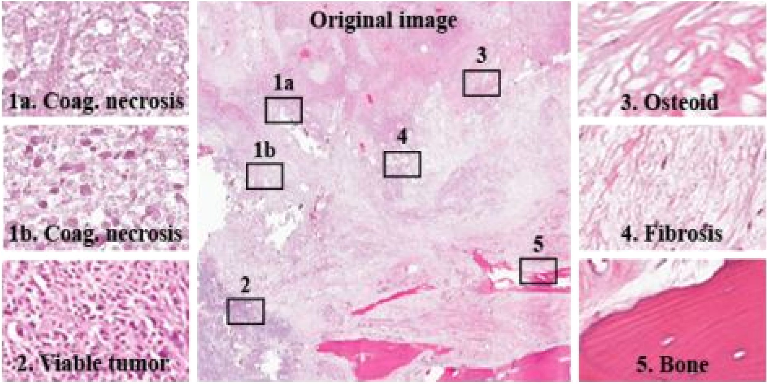
The figure shows different histological regions: viable tumor, coagulative necrosis, osteoid, fibrosis, and nontumor (bone) regions in a slide.

1.1.1. Tumor necrosis

Pollheimer et al. (2010) showed that the percentage of tumor necrosis has significant impact on the prognosis of colorectal cancer patients. In osteosarcoma, prognostic markers for survival are defined by the histopathological evaluation of post-chemotherapy osteosarcoma specimens (Rosen et al., 1979). The percent of necrosis can be utilized as a predictor for local control of osteosarcoma and also for the event free and overall survival in patients with non-metastatic disease. The pathological evaluation for the calculation of % necrosis begins with measurements and the analysis of bisected bone segments. The pathologists use sectioned slides to assess the aggregate tumor necrosis. According to the pathologists, more than 90% necrosis is considered favorable for long-term survival.

1.2. Related work

Histopathology image analysis is a gold standard for cancer recognition and diagnosis. In recent years, usage of digital histopathology has shown tremendous growth and promise. Irshad et al. (2014), in their paper, present a survey on existing work for analysis of histopathology images involving thresholding with region growing, k means, and morphological features such as area and shape structures. Arunachalam et al. (2016) presented multi-level Otsu thresholding followed by shape segmentation to identify viable tumor, necrosis, and nontumor regions in osteosarcoma histology slides.

Although there is only some research done in the analysis of osteosarcoma histology slides, research has proved that machine-learning approaches have started to become the state of the art in image classification and segmentation of other types of cancer, such as breast cancer, prostate cancer, or brain tumor. Most of these tumor studies focus on identifying a super-set of features, although not all features are relevant. A recent study on non-small cell lung cancer (Yu et al., 2016) isolated 9000+ features from images, which consisted of parameters extracted from color, texture, object identification, granularity, density, etc.

Cireşan et al. (2013) were the pioneers of utilizing CNN in mitosis counting for primary breast cancer grading. Litjens et al. (2016) applied CNN for identifying breast cancer metastases in sentinel lymph nodes and prostate cancer detection. Malon et al. (2013) trained a CNN to classify mitotic and non-mitotic cells by using morphological features such as color, texture, and shape. In Li et al. (2017), deep CNN was used along with data augmentation to segment gliomas and obtained a dice similarity of 0.88. Su et al. (2015) used a fast-scanning deep CNN for region segmentation and classification in breast cancer, and Spanhol et al. (2016) developed on existing AlexNet for different segmentation and classification tasks in breast cancer.

All of the methods mentioned earlier are focused on nuclei or region segmentation and not on image classification as tumor or nontumor, but recent studies by Li et al. (2014) have shown that CNN gives promising results for image patch classification.

In this article, we propose a deep learning approach that is capable of assigning tumor classes (viable tumor, necrosis) versus nontumor directly to input slides in osteosarcoma, a type of cancer with significantly more variability in tumor description. Our proposed architecture is an extension of the successful Alexnet architecture proposed by Krizhevsky et al. (2012) and the LeNet network architecture introduced by LeCun et al. (1998), which uses gradient-based learning with the back propagation algorithm.

1.3. Challenges

Some key challenges in automatic analysis of osteosarcoma histology images include:

1. Complexity and diversity of image data: This refers to the difficulty in representing the histology images with common features and patterns. Osteosarcoma has a high degree of heterogeneity (Fig. 1). The histology images exhibit diverse cellular morphology, texture, shape, and color variations, which makes finding a general pattern for tumor identification difficult.

2. Size of a single whole slide histopathology image: The large sizes of individual histology slides increase the computation complexity and require high computational resources. A single WSI can contain up to 100,000 × 100,000 pixels, and usually each patient will have around 25 scanned slides. Due to the large-scale dataset, the model used to analyze it should be time and memory efficient.

3. Availability of training data: Another major concern is the availability and quality of training data. Detailed manual annotation of medical images requires a great deal of time and effort. Also, many clinical features are hard to quantify, causing manual annotation to be intrinsically ambiguous, even if labeled by clinical experts. Moreover, the training data acquired can be imbalanced and biased toward one class instance.

1.3.1. Our contribution

Our main contribution is a new, important, practical, and efficient application of CNN, which gives promising results in osteosarcoma image classification. We developed an efficient CNN architecture used to classify the input images into tumor classes through the use of data augmentation techniques that save time and space. This work done for osteosarcoma image patch classification using CNN is the first work of this kind to the best of our knowledge. We also provide comparative results of our proposed architecture with three existing architectures: AlexNet, Lenet, and VGGNet (Simonyan and Zisserman, 2014) to show that the proposed architecture performs better in osteosarcoma tumor classification. In the end, we calculate the percentage necrosis by counting the number of patches classified as necrotic by our model for one WSI.

2. Our Approach

In this section, we describe the baseline CNN architecture proposed in Mishra et al. (2017). We follow it by describing the approach taken to improve and to extend the baseline to get better results.

2.1. Convolutional neural network

CNNs are powerful tools in deep learning with a high success rate in image classification. The typical CNN architecture for image classification consists of a series of convolution filters paired with pooling layers. The convolution filters are applied to small patches of the input image to detect increasingly relevant image features, such as edges or shapes and texture. The output of the CNN is one or more probabilities or class labels. According to Sirinukunwattana et al. (2016), “Mathematically, CNN can be defined as a feed forward artificial neural network C which is composed of L layers \documentclass{aastex}\usepackage{amsbsy}\usepackage{amsfonts}\usepackage{amssymb}\usepackage{bm}\usepackage{mathrsfs}\usepackage{pifont}\usepackage{stmaryrd}\usepackage{textcomp}\usepackage{portland, xspace}\usepackage{amsmath, amsxtra}\usepackage{upgreek}\pagestyle{empty}\DeclareMathSizes{10}{9}{7}{6}\begin{document} $$\left( {{C_1} , {C_2} , \ldots , {C_L}} \right)$$ \end{document} that maps an input vector x to an output vector y i.e \documentclass{aastex}\usepackage{amsbsy}\usepackage{amsfonts}\usepackage{amssymb}\usepackage{bm}\usepackage{mathrsfs}\usepackage{pifont}\usepackage{stmaryrd}\usepackage{textcomp}\usepackage{portland, xspace}\usepackage{amsmath, amsxtra}\usepackage{upgreek}\pagestyle{empty}\DeclareMathSizes{10}{9}{7}{6}\begin{document} \begin{align*} y = f \left( {x;{w_1} , {w_2} , \ldots , {w_L}} \right) = {f_L} \left( {;{w_L}} \right) \circ {f_{L - 1}} \left( {;{w_{L - 1}}} \right) \circ \cdots \circ {f_1} \left( {x;{w_1}} \right) , \tag{1} \end{align*} \end{document}

where w_l is the weight and bias vector for the lth layer f_l.”

Our approach is conceptually simple. It directly operates on raw RGB data sampled from the source. It is trained to classify patches into three bins: viable tumor, necrosis (coagulative necrosis, osteoid, fibrosis), and nontumor. Classification in unseen images is done by applying the learned classifier as a sliding window to the data. Because the CNN operates on raw pixel values, no human input is needed besides the initial annotation of slides for training data, a significant advantage over previous attempts (Arunachalam et al., 2016). The CNN automatically learns a set of visual features from the training data.

We develop on existing proven networks LeNet and AlexNet because finding a successful network configuration for a given problem can be a difficult challenge given the total number of possible configurations that can be defined. The Lenet architectures (LeCun et al., 1998) have been prototypes for many successful applications in image processing, particularly handwriting recognition and face detection. The data augmentation methods to reduce over-fitting on image data as described by Krizhevsky et al. (2012) have been proclaimed for their success rate in various object recognition applications.

2.2. Convolutional neural network architecture

2.2.1. Convolutional neural network design

Designing the architecture of a neural network is a complex task. A simple three-layer network has the following layers:

1. Input: This will hold the raw pixel values of the image, that is, an image of width 128, height 128, and with three color channels R,G,B. The input volume is [128 × 128 × 3].

2. Convolution: This layer will compute the output of neurons that are connected to local regions in the input image. Each neuron will compute the dot product between their weights and a small region that they are connected to in the input volume. This may result in volume such as [124 × 124 × 4] for four filters.

3. Max pooling: This layer will down-sample along the spatial dimensions (width, height), resulting in volume [62 × 62 × 4].

4. Multi-level perceptron: The multi-perceptron layer will compute the class scores, resulting in volume of size [1 × 1 × 3], where each of the three numbers corresponds to a class score for the three tumor regions.

2.2.2. Baseline architecture

For this article, we considered the three convolution layer CNN defined in Mishra et al. (2017) as the baseline architecture and worked on top of that. It was a simple neural network that was not able to identify all the features, and the output classification accuracy was very low. This leads to the requirement of increasing the number of hidden layers in the network. But inclusion of many hidden layers can increase the training time and memory requirements with little improvement in performance, making the network impractical. Hence, a trade-off is needed between efficiency and accuracy. In the previous paper (Mishra et al., 2017), different numbers of hidden layers were added without any changes to the hyper-parameters. It was noticed that there was a big jump in the accuracy from a one-convolutional layer to a three-convolutional layer architecture (Table 1).

Table 1.

Comparison of Accuracy and Running Time for Three Different Baseline Implementations of Neural Network with Different Number of Hidden Layers

Architecture	Accuracy	Running time (minutes)
1 convolution	0.21	3
3 convolution	0.86	18
Baseline Architecture	0.84	7

The detailed architecture of the three convolution CNN for tumor classification is shown in Fig. 3. The architecture combined the simplicity of Lenet architecture with the data augmentation methods used by AlexNet architecture. The lower three layers comprised alternating convolution and max-pooling layers. The first convolution layer has a filter size 5 × 5 that is used to detect low-level features such as edges, and it is followed by a max-pooling layer of scale 2 to down-sample the data. These data are then sent to the second layer of 5 × 5 filters to detect higher-order features such as texture and spatial connectivity followed by a max-pooling layer. The last convolution layer uses a filter of size 3 × 3 and max-pooling size 2 for down-sampling to generate more higher-order features. The upper two layers are fully connected multi-level perceptron (MLP) neural network (hidden layer+logistic regression). The second layer of the MLP is the output layer consisting of four neurons (Table 2). The input to the first MLP layer is the set of all features maps at the layer below and the output is a class probability distribution from the three neurons (p₁, p₂, p₃) for each image, where p₁, p₂, and p₃ are the probability for viable tumor, necrosis, and nontumor, respectively. The sum of the output probabilities from the MLP is 1, ensured by the use of Softmax algorithm as the activation function in the output layer of the MLP. The convolution and max-pooling layers are feature extractors, and the MLP is the classifier.

FIG. 3.

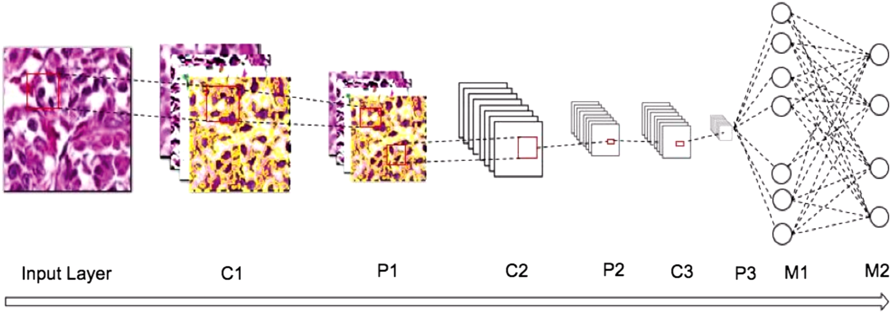
The figure shows the architecture of a convolution neural network for the classification of osteosarcoma. The different layers in the network are three convolution layers (C), three sub-sampling layers (P), and two fully connected multi-level perceptrons (M).

Table 2.

Architecture of the Baseline Convolutional Neural Network for Osteosarcoma Classification

Layer	Type	Filter size	Output size
0	I		128 × 128
1	C	5 × 5	124 × 124
2	P	2 × 2	62 × 62
3	C	5 × 5	58 × 58
4	P	2 × 2	29 × 29
5	C	3 × 3	27 × 27
6	P	2 × 2	14 × 14
7	M	32	1 × 32
8	M		1 × 4

The network is built of Input (I), Convolution (C), Max-Pooling (P), and fully connected (M) layers.

2.2.3. Extended architecture

The average accuracy achieved by the baseline architecture was 84%. Useful evaluation of histology slides cannot depend on this accuracy with a high confidence, hence there was a need to improve the architecture for better classification results. The first step to increase accuracy and get better feature extraction was to increase the number of hidden layers. The filter size was decreased from 5 × 5 to 3 × 3 to make the network deep and to allow for nonlinearities, which allowed to stack two 3 × 3 filters instead of a single 5 × 5 filter. This is advantageous as having only one 5 × 5 layer will compute a linear function over the input volume, whereas the stacked 3 × 3 filter will contain nonlinearities that will make the extracted features more expressive. Also, for the stacked 3 × 3 filters, the two-convolutional layer will contain \documentclass{aastex}\usepackage{amsbsy}\usepackage{amsfonts}\usepackage{amssymb}\usepackage{bm}\usepackage{mathrsfs}\usepackage{pifont}\usepackage{stmaryrd}\usepackage{textcomp}\usepackage{portland, xspace}\usepackage{amsmath, amsxtra}\usepackage{upgreek}\pagestyle{empty}\DeclareMathSizes{10}{9}{7}{6}\begin{document} $$2 \times ( C \times [ 3 \times 3 \times C ] ) = 18{C^2}$$ \end{document} parameters whereas a single 5 × 5 filter convolutional layer will have \documentclass{aastex}\usepackage{amsbsy}\usepackage{amsfonts}\usepackage{amssymb}\usepackage{bm}\usepackage{mathrsfs}\usepackage{pifont}\usepackage{stmaryrd}\usepackage{textcomp}\usepackage{portland, xspace}\usepackage{amsmath, amsxtra}\usepackage{upgreek}\pagestyle{empty}\DeclareMathSizes{10}{9}{7}{6}\begin{document} $$C \times ( 5 \times 5 \times C ) = 25{C^2}$$ \end{document} parameters. Here, C is the number of channels, which is 3. Thus, two layers of convolutional filters have 163 parameters and a single 5 × 5 filter has 225 parameters. This shows that stacking convolutional layers with smaller filter sizes expresses more powerful features with fewer parameters.

Using this principle, the baseline CNN was extended by replacing each 5 × 5 convolutional layer with two 3 × 3 stacked convolutional layers. Stride 1 is used so that most of the spatial down-sampling is done by the max-pooling layers, with the convolutional layers only transforming the input volume depth wise. All hidden layers are followed with an ReLU (Rectified Linear Unit) as the activation function layer. Each stack of two convolution+ReLU is followed by spatial pooling through the max-pooling layer. The updated architecture is shown in Table 3. Another change to the extended architecture was to do a three-class classification instead of a four-class classification. The advantage of this step is explained in later sections. The average output accuracy of the neural network improved considerably with these changes to the architecture as shown in Table 4.

Table 3.

Architecture of the Extended Convolutional Neural Network for Osteosarcoma Patch Classification

Layer	Type	Filter size	No. of feature maps	Output size
0	I			128 × 128
1	C	3 × 3	64	124 × 124
2	C	3 × 3	64	120 × 120
3	P	2 × 2	64	60 × 60
4	C	3 × 3	128	56 × 56
5	C	3 × 3	128	52 × 52
6	P	2 × 2	128	26 × 26
7	C	3 × 3	256	24 × 24
8	C	3 × 3	256	22 × 22
9	M		1024	1 × 1024
10	M		1024	1 × 1024
11	M		3	1 × 3

The network is built of Input (I), Convolution+ReLU (C), Max-Pooling (P), and fully connected (M) layers.

ReLU, Rectified Linear Unit.

Table 4.

Comparison of Accuracy of Different Classes for Baseline Implementation of Neural Network with the Extended Version

Architecture	Viable	Necrosis	Nontumor
Baseline architecture	0.83	0.73	0.91
Extended architecture	0.92	0.90	0.95

2.2.4. Data preprocessing

The output of the neural network is highly dependent on the input passed to it. Two distinct preprocessing steps were taken to generalize the training data for the neural network.

1. To alleviate the effect of illumination and contrast conditions while scanning the histology slides, the RGB channel input was transformed into Lab color space. Normalization was done on the L (lightness) parameter of the Lab space.

2. To make the training data aware of contextual information, for each 128 × 128 image tile, a larger area of 1024 × 1024 was added to the training data. This larger area was reduced to the 128 × 128 size by bi-linear interpolation. This was done to make the model contextual independent.

3. To keep the training data balanced and only with images having relevant data, all the images in the training set are processed in a shredder program that removes images containing only white pixels or empty background pixels from the set.

2.2.5. Data augmentation

The easiest and most common method to reduce over-fitting of data is to artificially augment the dataset by using label-preserving transformations. We use two distinct data augmentation techniques, both of which allow transformed images to be produced from the original images with very little computation, so the transformed images do not need to be stored on disk. This is a significant saving in both space and time, since WSI images are huge in size and disk read/write is a time-consuming process. For this purpose, first we arbitrarily rotate the training images by (0°, 90°, 180°, 270°) and flip them along the vertical and horizontal axis to ensure that the network does not learn any rotation-dependent features. The second technique for data augmentation alters the intensities of the RGB channels in training images (Krizhevsky et al., 2012). We perform principal component analysis (PCA) on the set of RGB pixel values throughout the training set and then, for each training image, we add to each RGB image pixel (i.e., \documentclass{aastex}\usepackage{amsbsy}\usepackage{amsfonts}\usepackage{amssymb}\usepackage{bm}\usepackage{mathrsfs}\usepackage{pifont}\usepackage{stmaryrd}\usepackage{textcomp}\usepackage{portland, xspace}\usepackage{amsmath, amsxtra}\usepackage{upgreek}\pagestyle{empty}\DeclareMathSizes{10}{9}{7}{6}\begin{document} $${I_{xy}} = [ I_{xy}^R , I_{xy}^G , I_{xy}^B{ ] ^T}$$ \end{document} ), the quantity \documentclass{aastex}\usepackage{amsbsy}\usepackage{amsfonts}\usepackage{amssymb}\usepackage{bm}\usepackage{mathrsfs}\usepackage{pifont}\usepackage{stmaryrd}\usepackage{textcomp}\usepackage{portland, xspace}\usepackage{amsmath, amsxtra}\usepackage{upgreek}\pagestyle{empty}\DeclareMathSizes{10}{9}{7}{6}\begin{document} $$[ {p_1} , {p_2} , {p_3} ] [ { \alpha _1}{ \lambda _1} , { \alpha _2}{ \lambda _2} , { \alpha _3}{ \lambda _3}{ ] ^T}$$ \end{document} , where p_i and \documentclass{aastex}\usepackage{amsbsy}\usepackage{amsfonts}\usepackage{amssymb}\usepackage{bm}\usepackage{mathrsfs}\usepackage{pifont}\usepackage{stmaryrd}\usepackage{textcomp}\usepackage{portland, xspace}\usepackage{amsmath, amsxtra}\usepackage{upgreek}\pagestyle{empty}\DeclareMathSizes{10}{9}{7}{6}\begin{document} $${ \lambda _i}$$ \end{document} are the i-th eigenvector and eigenvalue of the 3 × 3 covariance matrix of RGB pixel values, respectively, and \documentclass{aastex}\usepackage{amsbsy}\usepackage{amsfonts}\usepackage{amssymb}\usepackage{bm}\usepackage{mathrsfs}\usepackage{pifont}\usepackage{stmaryrd}\usepackage{textcomp}\usepackage{portland, xspace}\usepackage{amsmath, amsxtra}\usepackage{upgreek}\pagestyle{empty}\DeclareMathSizes{10}{9}{7}{6}\begin{document} $${ \alpha _i}$$ \end{document} is a random variable drawn from a Gaussian with mean 0 and standard deviation 0.1. Data augmentation helps alleviate over-fitting by considerably increasing the amount of training data, removing rotation dependency, and making the training images invariant to changes in the color brightness and intensity through PCA (Fig. 4).

FIG. 4.

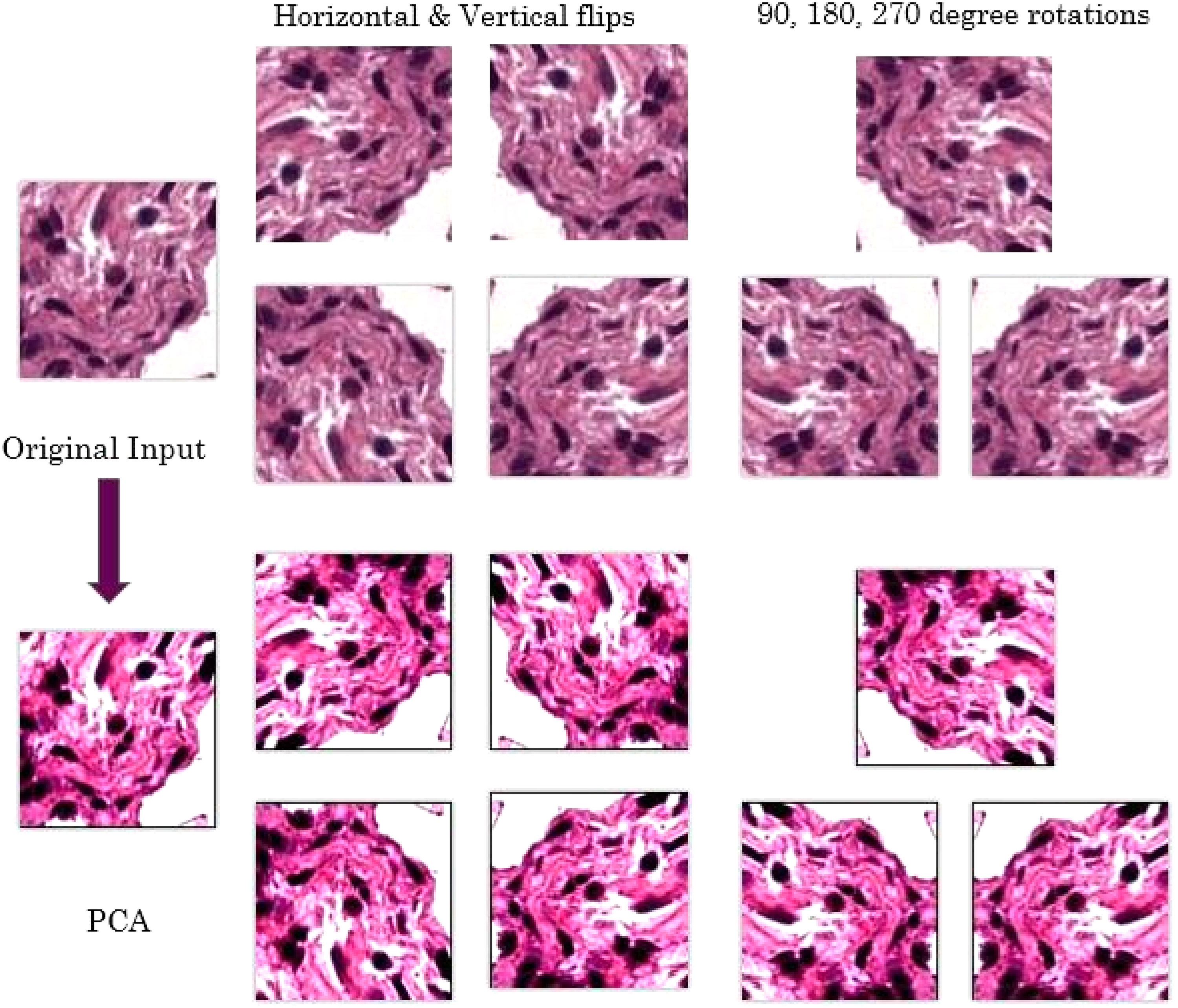
The figure shows the different data augmentation applied to the training set.

2.2.6. Initialization and training

The network is trained with stochastic gradient descent. All weights are initialized with 0 mean by assigning them small, random, and unique numbers from \documentclass{aastex}\usepackage{amsbsy}\usepackage{amsfonts}\usepackage{amssymb}\usepackage{bm}\usepackage{mathrsfs}\usepackage{pifont}\usepackage{stmaryrd}\usepackage{textcomp}\usepackage{portland, xspace}\usepackage{amsmath, amsxtra}\usepackage{upgreek}\pagestyle{empty}\DeclareMathSizes{10}{9}{7}{6}\begin{document} $${10^{ - 2}}$$ \end{document} standard deviation Gaussian random numbers, so that each layer calculates unique updates and integrates itself as a different unit of the full network. The network uses gradient descent to calculate weights with Adam optimization (Kingma and Ba, 2014) to handle the sparse gradient updates caused by the training input.

3. Experimental Setup

3.1. Data

In digital histopathology, the H&E stained microscopic slides are scanned by using powerful slidescanner software, such as Aperio, and converted to digital WSIs. Each WSI supports upto 40 × magnification, capturing bones, tissues, cellular and sub-cellular structures such as nuclei and cytoplasm. A patient case can consist of an average of 25 individual WSI images representing different sections of the microscopic slide. Pathologists manually selected 82 WSIs from 50 patient cases to capture the tumor variability. From each of these 82 patient WSIs, 25–30 random tiles of size 1024 by 1024 were selected by a program. A total of 1000 tiles that represent different tissue and cellular regions with appearance of both normal and tumor regions were identified for training and testing purposes. For the network to learn the correct representation of tumor, it is important that the training data contain enough information to allow discrimination between the different tissue and cellular structures present in the tiles. As such, the correct resolution used for tile generation was determined through discussions with senior pathologists and was fixed at 10 × , which was then used to generate the random tiles.

The pathologists then used an in-house tool that we developed to annotate these 1000 tiles as viable tumor, nonviable tumor (coagulative necrosis, osteoid, fibrosis), and nontumor. As it is difficult to feed 1024 × 1024 tiles to the neural network, we cropped and segmented the 1024 × 1024 image into smaller patches for training. Patch size was determined through initial trial runs on the network. The 256 × 256 patches limited the CNN due to memory issues, and the 64 × 64 patch size had very low accuracy. Hence, we decided on a 128 × 128 patch size. This resulted in about 64,000 image patches in the dataset. To alleviate contextual dependency, the 1024 × 1024 images were used in the training set by resizing them to 128 × 128 size. The 128 by 128 patch generation was done manually based on the pathologist's annotation of the tiles. This manual generation of patches helped differentiating annotations of different regions in a tile. In the baseline architecture (Mishra et al., 2017), a patch can consist of more than one class and a four-class classifier was used to handle multi-class patches. The manual generation of patches allowed for a three-class classification as it ensures that every patch contains only one type of class. All the 128 × 128 patches were processed to remove images containing only white or background pixels. Table 5 shows the data distribution among the various classes. Only 60% of the patches were used for training, 20% data were used as a validation set, and the remaining 20% data were used for the test set. Figure 5 shows some example patches in the training set.

FIG. 5.

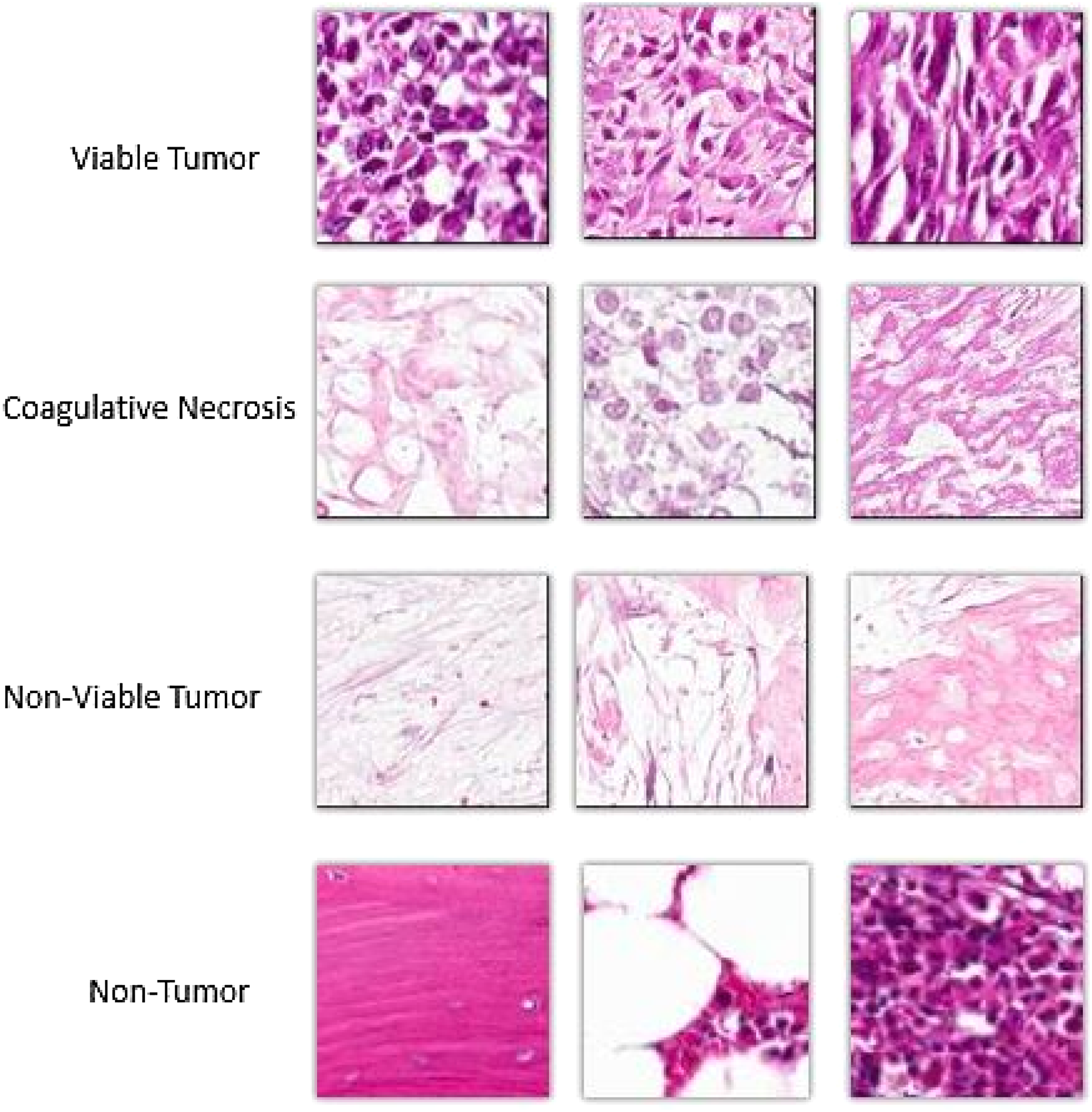
Example patches of different types of regions found in the dataset.

Table 5.

Data Distribution

Tumor type	No. of annotated tiles (size 1024 × 1024)	No. of annotated patches (size 128 × 128)	No. of training patches (size 128 × 128)	No. of test patches (size 128 × 128)
Viable tumor (for tiles includes multi-class tiles)	312	19,776	11,866	3955
Necrosis	268	17,344	10,406	3469
Nontumor	420	26,880	16,128	5376

3.2. Implementation

We used existing open-source libraries to implement the neural network architecture. The architecture was developed in JAVA by using dl4j (deep learning for java) libraries (Gibson, 2017). The training data were fed to the network in batch sizes of 100 to utilize parallelism and improve the network efficiency through graphical processing unit (GPU) utilization. The preprocessing programs and the annotation application were developed in JAVA.

4. Results

4.1. Evaluation

The objective of the network was to classify the input images tiles into one of the three regions (viable tumor, necrosis, nontumor) as mentioned in the previous sections. The output of the neural network is a probability distribution with sum 1. The output class is the class with the highest probability. The regions coagulative necrosis, osteoid, and fibrosis all fall into class necrosis. The performance of the neural network was monitored by assessing the error rate on the validation set. Once the error rate saturated after 10 epochs, training was stopped. The total training time for our implementation of the network was around 15 minutes.

We evaluate the accuracy of the proposed method quantitatively by using accuracy A = (True Positives + True Negatives)/(Total Sample Size), precision P = (True Positives)/(True Positives + False Positives), recall R = (True Positives)/(True Positives + False Negatives), and F1-Score F₁ = (2PR)/(P + R). Our implementation gives an average accuracy of 0.924.

4.2. Comparative results

The output of a neural network is dependent on the architecture of the network. Different architectures, with different depths and/or numbers of units in the hidden layers, result in different output. Shallower networks with fewer number of hidden units are more resistant to over-fitting, require less training data, and train faster per example but can result in loss of precision due to lack of higher-order features. A deeper network with more hidden units may be able to learn patterns from the training data more precisely but could result in over-fitting of the data and loss of efficiency. In this section, we present and compare the qualitative output of four architectures: AlexNet, Lenet, VGGNet (Simonyan and Zisserman, 2014), and our proposed architecture. We find that the running time of Lenet is fastest but the accuracy and precision of our proposed architecture is better than all the other architectures (Table 6).

Table 6.

Comparison of Accuracy, Precision, Recall, and F1-Score for Different Architectures

Architecture	Accuracy	Precision	Recall	F1-score
AlexNet	0.73	0.81	0.75	0.78
LeNet	0.67	0.75	0.67	0.71
VGGNet	0.67	0.75	0.67	0.71
Baseline architecture	0.84	0.89	0.84	0.86
Proposed architecture	0.924	0.97	0.94	0.95

Arunachalam et al. (2016) used a multi-level Otsu threshold and clustering algorithms to segment out viable-tumor, necrosis, and nonviable tumor regions. The accuracy of the method was around 90% for the limited data set used in that paper, but the accuracy dropped to 60% for the updated test dataset. It can be argued that the results are prone to over-fitting and may not generalize well for other datasets, whereas the neural network learns the features through the input images and thus can avoid over-fitting, while also becoming better once more data are fed in.

We used the Receiver-Operator-Characteristic (ROC) curve (Fig. 6) to compare our model results with other networks. In an ROC curve, the true positive rate (Sensitivity) is plotted as a function of the false positive rate (100-Specificity) for different cut-off points. Each point on the ROC curve represents a sensitivity/specificity pair corresponding to a particular decision threshold. A test with perfect discrimination (no overlap in the two distributions) has an ROC curve that passes through the upper left corner (100% sensitivity, 100% specificity). Therefore, the closer the ROC curve is to the upper right corner, the higher the overall accuracy of the test (Hajian-Tilaki, 2013).

FIG. 6.

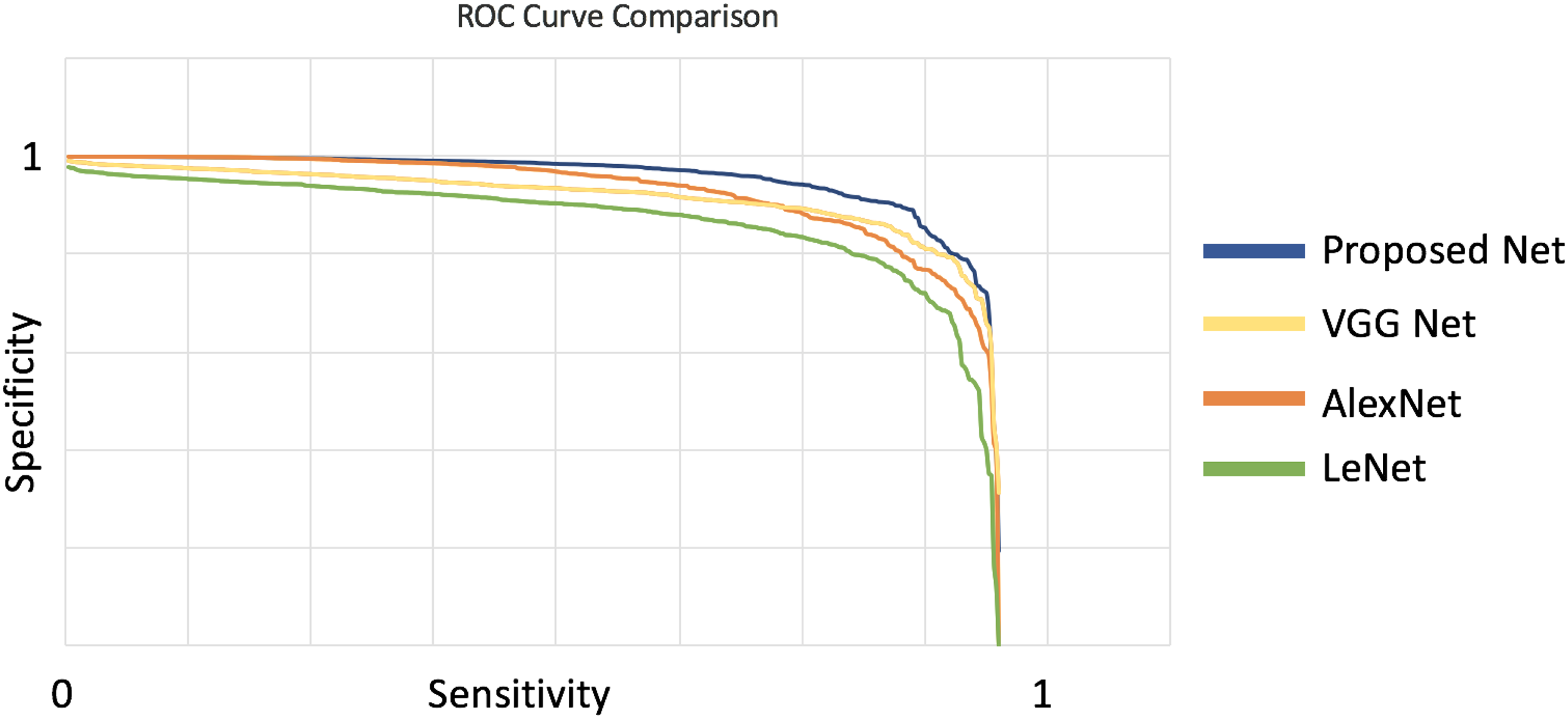
Comparison between the ROC curve of different networks. We see that the proposed network will have a higher accuracy as the curve is closer to the upper right corner. ROC, receiver-operator-characteristic.

4.2.1. Necrosis calculation

The final goal for osteosarcoma evaluation is calculating the percentage of necrosis in a given WSI. To this purpose, for a WSI image, we divide it into patches of 128 × 128, and we send these patches to the learned model for classification. We then count the number of patches that were classified as necrotic to output the percentage of necrosis in any give WSI. The complete pipeline for tumor necrosis calculation for osteosarcoma is shown (Fig. 7).

FIG. 7.

The pipeline for necrosis percentage calculation.

5. Conclusion

In this article, we proposed a deep learning approach using CNN for tumor classification in osteosarcoma. The proposed method is efficient and accurate and focuses on class-level identification instead of nuclei level. The training and evaluation was done on a dataset manually annotated by senior pathologists. As far as the authors are aware, this is the first journal article describing the applicability of CNNs for diagnostic analysis of osteosarcoma. We have shown that the technique has high potential to improve the diagnostic process and to be used as a clinical tool in osteosarcoma analysis.

The architecture of the CNN proposed in this article was chosen on the basis of datasets and resources available. Justifying any architecture through theory is an ongoing research. A deeper network architecture will allow for more variations in the input but will cost more resources. We can continue to explore different architectures and strategies for the training of a neural network by changing the hyper-parameters or using the architecture for feature extraction and classifying only on the basis of relevant features.

Footnotes

Acknowledgments

This research was partially supported by CPRIT award RP150164. The authors would like to thank John-Paul Bach, Molly and Sammy Glick from UT Southwestern Medical Center and Maria Martinez from UT Dallas for their help with the datasets.

Author Disclosure Statement

No competing financial interests exist.

References

Arunachalam

H.B.

, Mishra

, Armaselu

, et al. 2016. Computer aided image segmentation and classification for viable and non-viable tumor identification in osteosarcoma. Pac. Symp. Biocomput., 22, 195–206.

Cireşan

D.C.

, Giusti

, Gambardella

L.M.

, et al. 2013. Mitosis detection in breast cancer histology images with deep neural networks. Med. Image Comput. Comput. Assist. Interv., 16, 411–418.

Fischer

A.H.

, Jacobson

K.A.

, Rose

, et al. 2008. Hematoxylin and eosin staining of tissue and cell sections. Cold Spring Harbor Protoc. 2008, pdb.prot4986.

Fuchs

T.J.

, Wild

P.J.

, Moch

, et al. 2008. Computational pathology analysis of tissue microarrays predicts survival of renal clear cell carcinoma patients. Med. Image Comput. Comput. Assist. Interv., 11, 1–8.

Gibson

C.N.A.

(n.d.). Deeplearning4j Development Team. Deeplearning4j: Open-source distributed deep learning for the JVM. Apache Software Foundation license 2.0. http://deeplearning4j.org. Retrieved: June 18, 2017.

Goode

, Gilbert

, Harkes

, et al. 2013. Openslide: A vendor-neutral software foundation for digital pathology. J. Pathol. Inform. 4, 27.

Hajian-Tilaki

2013. Receiver operating characteristic (ROC) curve analysis for medical diagnostic test evaluation. Caspian J. Intern. Med. 4, 627.

Irshad

, Veillard

, Roux

, et al. 2014. Methods for nuclei detection, segmentation, and classification in digital histopathology: A review—current status and future potential. IEEE Rev. Biomed. Eng. 7, 97–114.

Kingma

, and Ba

2014. Adam: A method for stochastic optimization. arXiv 1412.6980.

10.

Kothari

, Phan

J.H.

, Stokes

T.H.

, et al. 2013. Pathology imaging informatics for quantitative analysis of whole-slide images. J. Am. Med. Inform. Assoc. 20, 1099–1108.

11.

Krizhevsky

, Sutskever

, and Hinton

G.E.

2012. Imagenet classification with deep convolutional neural networks. Adv. Neural Inf. Process. Syst. 1097–1105.

12.

LeCun

, Bottou

, Bengio

, et al. 1998. Gradient-based learning applied to document recognition. Proc. IEEE, 86, 2278–2324.

13.

, Cai

, Wang

, et al. 2014. Medical image classification with convolutional neural network. Presented at 2014 13th International Conference on Control Automation Robotics & Vision (ICARCV), Marina Bay Sands, Singapore, 844–848.

14.

, Wang

, Yu

, et al. 2017. Low-grade glioma segmentation based on CNN with fully connected CRF. J. Healthc. Eng. Vol. 2017, article ID: 9283480, 12 pgs.

15.

Litjens

, Sánchez

C.I.

, Timofeeva

, et al. 2016. Deep learning as a tool for increased accuracy and efficiency of histopathological diagnosis. Sci. Rep., 6:26286.

16.

Malon

C.D.

, Cosatto

, et al. 2013. Classification of mitotic figures with convolutional neural networks and seeded blob features. J. Pathol. Inform. 4, 9.

17.

Mishra

, Daescu

, Leavey

, et al. 2017. Histopathological diagnosis for viable and non-viable tumor prediction for osteosarcoma using convolutional neural network. Presented at International Symposium on Bioinformatics Research and Applications, Waikiki Beach, HI, 12–23.

18.

Ottaviani

, and Jaffe

2009. The epidemiology of osteosarcoma. In: Jaffe

, Bruland

, and Bielack

, eds. Pediatric and Adolescent Osteosarcoma. Canc. Treat. Res., vol. 152. Springer, Boston, MA.

19.

Pollheimer

M.J.

, Kornprat

, Lindtner

R.A.

, et al. 2010. Tumor necrosis is a new promising prognostic factor in colorectal cancer. Hum. Pathol. 41, 1749–1757.

20.

Rosen

, Marcove

R.C.

, and Caparros

1979. The rationale for preoperative chemotherapy and delayed surgery. Cancer, 43, 2163–2177.

21.

Simonyan

, and Zisserman

2014. Very deep convolutional networks for large-scale image recognition. arXiv 1409.1556.

22.

Sirinukunwattana

, Raza

S.E.A.

, Tsang

Y.-W.

, et al. (2016). Locality sensitive deep learning for detection and classification of nuclei in routine colon cancer histology images. IEEE Trans. Med. Imaging., 35, 1196–1206.

23.

Spanhol

F.A.

, Oliveira

L.S.

, Petitjean

, et al. 2016. Breast cancer histopathological image classification using convolutional neural networks. Presented at 2016 International Joint Conference on Neural Networks (IJCNN), Vancouver, Canada, 2560–2567.

24.

, Liu

, Xie

, et al. 2015. Region segmentation in histopathological breast cancer images using deep convolutional neural network. Presented at 2015 IEEE 12th International Symposium on Biomedical Imaging (ISBI), Brooklyn, NY, 55–58.

25.

K.-H.

, Zhang

, Berry

G.J.

, et al. 2016. Predicting non-small cell lung cancer prognosis by fully automated microscopic pathology image features. Nat. Commun. 7:12474.