Cryo-electron microscopy (cryo-EM) is a technique that produces three-dimensional density maps of large protein complexes. This allows for the study of the structure of these proteins. Identifying the secondary structures within proteins is vital to understanding the overall structure and function of the protein. The \documentclass{aastex}\usepackage{amsbsy}\usepackage{amsfonts}\usepackage{amssymb}\usepackage{bm}\usepackage{mathrsfs}\usepackage{pifont}\usepackage{stmaryrd}\usepackage{textcomp}\usepackage{portland, xspace}\usepackage{amsmath, amsxtra}\usepackage{upgreek}\pagestyle{empty}\DeclareMathSizes{10}{9}{7}{6}\begin{document}
$$\beta$$
\end{document}-barrel is one such secondary structure, commonly found in lipocalins and membrane proteins. In this article, we present a novel approach that utilizes genetic algorithms, kd-trees, and ray tracing to automatically detect and extract \documentclass{aastex}\usepackage{amsbsy}\usepackage{amsfonts}\usepackage{amssymb}\usepackage{bm}\usepackage{mathrsfs}\usepackage{pifont}\usepackage{stmaryrd}\usepackage{textcomp}\usepackage{portland, xspace}\usepackage{amsmath, amsxtra}\usepackage{upgreek}\pagestyle{empty}\DeclareMathSizes{10}{9}{7}{6}\begin{document}
$$\beta$$
\end{document}-barrels from cryo-EM density maps. This approach was tested on simulated and experimental density maps with zero, one, or multiple barrels in the density map. The results suggest that the proposed approach is capable of performing automatic detection of \documentclass{aastex}\usepackage{amsbsy}\usepackage{amsfonts}\usepackage{amssymb}\usepackage{bm}\usepackage{mathrsfs}\usepackage{pifont}\usepackage{stmaryrd}\usepackage{textcomp}\usepackage{portland, xspace}\usepackage{amsmath, amsxtra}\usepackage{upgreek}\pagestyle{empty}\DeclareMathSizes{10}{9}{7}{6}\begin{document}
$$\beta$$
\end{document}-barrels from medium resolution cryo-EM density maps.
1. Introduction
Cryo-electron microscopy (cryo-EM) is an experimental technique that allows for the study and imaging of the structure of large molecules and proteins (Adrian et al., 1984). Cryo-EM works by first freezing the molecule being studied. Next, numerous two-dimensional (2D) images of the molecule are taken, using an electron microscope, at different angles all around the molecule. These 2D images are then used to reconstruct a three-dimensional (3D) density map of the molecule (Khlbrandt, 2014). Since its initial introduction in the 1980s, cryo-EM has improved to the point of being able to resolve to near-atomic resolutions and identify individual atoms within the molecule being studied (Zhou, 2011; Ja et al., 2015; Mj et al., 2017).
However, there does exist a large amount of medium resolution (5 to 10 Å) cryo-EM data that have been produced (Lawson et al., 2011; Zhou, 2011). At these lower resolutions, individual atoms blur together and it is difficult to differentiate between individual atoms. However, at these lower resolutions, the blurring of the individual atoms instead allows the secondary structures within the protein to be clear and visible (Baker et al., 2007).
Secondary structures are local structures within proteins that combine to form the overall shape and structure of the protein. Because of this, it is important to be able to find and identify these secondary structures to understand a protein's function and mechanism. Secondary structures can be split up into two main categories: the \documentclass{aastex}\usepackage{amsbsy}\usepackage{amsfonts}\usepackage{amssymb}\usepackage{bm}\usepackage{mathrsfs}\usepackage{pifont}\usepackage{stmaryrd}\usepackage{textcomp}\usepackage{portland, xspace}\usepackage{amsmath, amsxtra}\usepackage{upgreek}\pagestyle{empty}\DeclareMathSizes{10}{9}{7}{6}\begin{document}
$$\alpha$$
\end{document}-helix and the \documentclass{aastex}\usepackage{amsbsy}\usepackage{amsfonts}\usepackage{amssymb}\usepackage{bm}\usepackage{mathrsfs}\usepackage{pifont}\usepackage{stmaryrd}\usepackage{textcomp}\usepackage{portland, xspace}\usepackage{amsmath, amsxtra}\usepackage{upgreek}\pagestyle{empty}\DeclareMathSizes{10}{9}{7}{6}\begin{document}
$$\beta$$
\end{document}-sheet.
The first type of secondary structure, \documentclass{aastex}\usepackage{amsbsy}\usepackage{amsfonts}\usepackage{amssymb}\usepackage{bm}\usepackage{mathrsfs}\usepackage{pifont}\usepackage{stmaryrd}\usepackage{textcomp}\usepackage{portland, xspace}\usepackage{amsmath, amsxtra}\usepackage{upgreek}\pagestyle{empty}\DeclareMathSizes{10}{9}{7}{6}\begin{document}
$$\alpha$$
\end{document}-helices, forms when a protein strand winds up into a helical structure. These regularly appear as a thick rod of density in medium resolution cryo-EM density maps. Because of this, \documentclass{aastex}\usepackage{amsbsy}\usepackage{amsfonts}\usepackage{amssymb}\usepackage{bm}\usepackage{mathrsfs}\usepackage{pifont}\usepackage{stmaryrd}\usepackage{textcomp}\usepackage{portland, xspace}\usepackage{amsmath, amsxtra}\usepackage{upgreek}\pagestyle{empty}\DeclareMathSizes{10}{9}{7}{6}\begin{document}
$$\alpha$$
\end{document}-helices are easier to identify from within the cryo-EM density maps and work has been done to successfully detect and isolate \documentclass{aastex}\usepackage{amsbsy}\usepackage{amsfonts}\usepackage{amssymb}\usepackage{bm}\usepackage{mathrsfs}\usepackage{pifont}\usepackage{stmaryrd}\usepackage{textcomp}\usepackage{portland, xspace}\usepackage{amsmath, amsxtra}\usepackage{upgreek}\pagestyle{empty}\DeclareMathSizes{10}{9}{7}{6}\begin{document}
$$\alpha$$
\end{document}-helices (Jiang et al., 2001; Dal Pal et al., 2006; Baker et al., 2007; Rusu and Wriggers, 2012; Si et al., 2012; Li et al., 2016).
In contrast, \documentclass{aastex}\usepackage{amsbsy}\usepackage{amsfonts}\usepackage{amssymb}\usepackage{bm}\usepackage{mathrsfs}\usepackage{pifont}\usepackage{stmaryrd}\usepackage{textcomp}\usepackage{portland, xspace}\usepackage{amsmath, amsxtra}\usepackage{upgreek}\pagestyle{empty}\DeclareMathSizes{10}{9}{7}{6}\begin{document}
$$\beta$$
\end{document}-sheets are formed when multiple \documentclass{aastex}\usepackage{amsbsy}\usepackage{amsfonts}\usepackage{amssymb}\usepackage{bm}\usepackage{mathrsfs}\usepackage{pifont}\usepackage{stmaryrd}\usepackage{textcomp}\usepackage{portland, xspace}\usepackage{amsmath, amsxtra}\usepackage{upgreek}\pagestyle{empty}\DeclareMathSizes{10}{9}{7}{6}\begin{document}
$$\beta$$
\end{document}-strands line up side by side to form a sheet-like structure. This generally shows up as a thin layer of density in medium resolution cryo-EM density maps. Like \documentclass{aastex}\usepackage{amsbsy}\usepackage{amsfonts}\usepackage{amssymb}\usepackage{bm}\usepackage{mathrsfs}\usepackage{pifont}\usepackage{stmaryrd}\usepackage{textcomp}\usepackage{portland, xspace}\usepackage{amsmath, amsxtra}\usepackage{upgreek}\pagestyle{empty}\DeclareMathSizes{10}{9}{7}{6}\begin{document}
$$\alpha$$
\end{document}-helices, work has been done to successfully detect the location and position of \documentclass{aastex}\usepackage{amsbsy}\usepackage{amsfonts}\usepackage{amssymb}\usepackage{bm}\usepackage{mathrsfs}\usepackage{pifont}\usepackage{stmaryrd}\usepackage{textcomp}\usepackage{portland, xspace}\usepackage{amsmath, amsxtra}\usepackage{upgreek}\pagestyle{empty}\DeclareMathSizes{10}{9}{7}{6}\begin{document}
$$\beta$$
\end{document}-strands (Si and He, 2013; Si and He, 2014; Li et al., 2016; Si and He, 2017). However, unlike \documentclass{aastex}\usepackage{amsbsy}\usepackage{amsfonts}\usepackage{amssymb}\usepackage{bm}\usepackage{mathrsfs}\usepackage{pifont}\usepackage{stmaryrd}\usepackage{textcomp}\usepackage{portland, xspace}\usepackage{amsmath, amsxtra}\usepackage{upgreek}\pagestyle{empty}\DeclareMathSizes{10}{9}{7}{6}\begin{document}
$$\alpha$$
\end{document}-helices, these \documentclass{aastex}\usepackage{amsbsy}\usepackage{amsfonts}\usepackage{amssymb}\usepackage{bm}\usepackage{mathrsfs}\usepackage{pifont}\usepackage{stmaryrd}\usepackage{textcomp}\usepackage{portland, xspace}\usepackage{amsmath, amsxtra}\usepackage{upgreek}\pagestyle{empty}\DeclareMathSizes{10}{9}{7}{6}\begin{document}
$$\beta$$
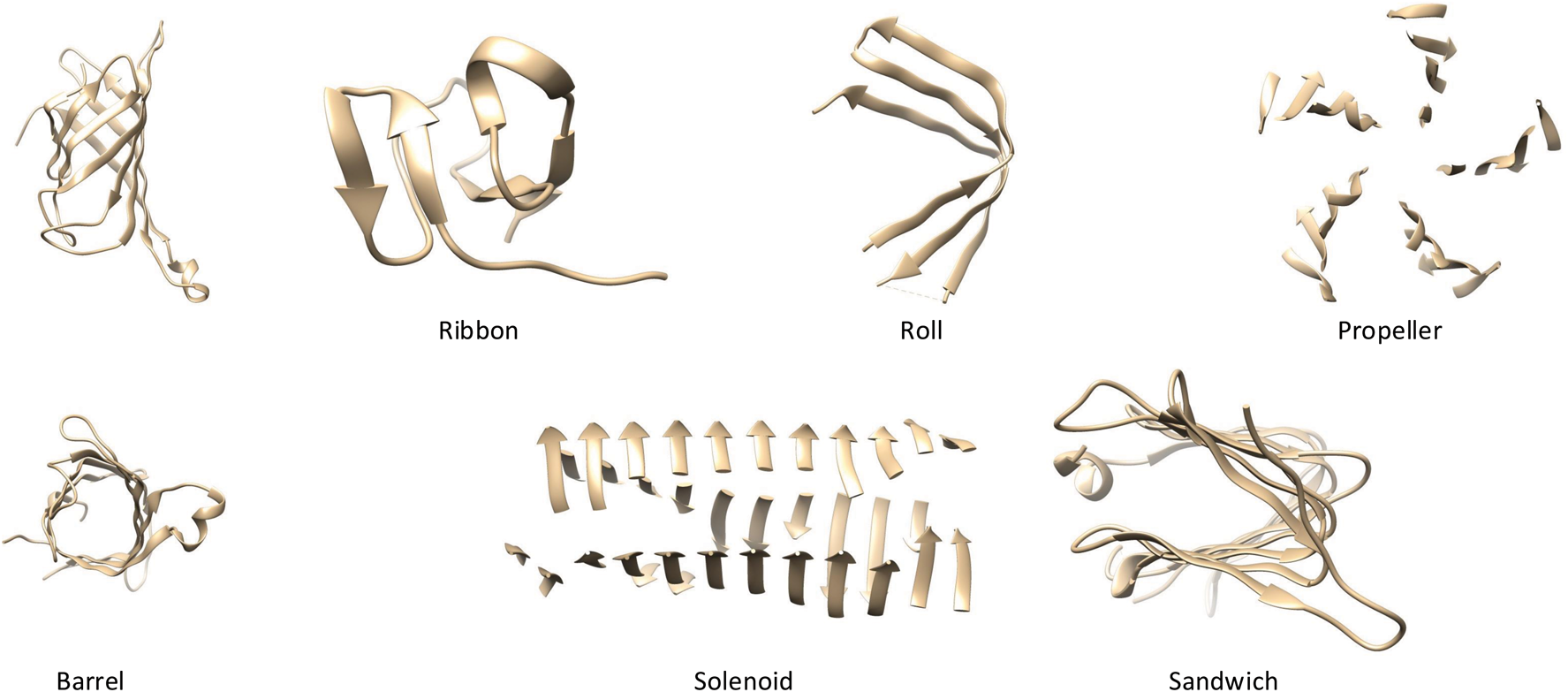
\end{document}-sheets can fold, twist, and combine to form many different shapes and geometries (Fig. 1).
Examples of various \documentclass{aastex}\usepackage{amsbsy}\usepackage{amsfonts}\usepackage{amssymb}\usepackage{bm}\usepackage{mathrsfs}\usepackage{pifont}\usepackage{stmaryrd}\usepackage{textcomp}\usepackage{portland, xspace}\usepackage{amsmath, amsxtra}\usepackage{upgreek}\pagestyle{empty}\DeclareMathSizes{10}{9}{7}{6}\begin{document}
$$\beta$$
\end{document}-sheet structures.
The \documentclass{aastex}\usepackage{amsbsy}\usepackage{amsfonts}\usepackage{amssymb}\usepackage{bm}\usepackage{mathrsfs}\usepackage{pifont}\usepackage{stmaryrd}\usepackage{textcomp}\usepackage{portland, xspace}\usepackage{amsmath, amsxtra}\usepackage{upgreek}\pagestyle{empty}\DeclareMathSizes{10}{9}{7}{6}\begin{document}
$$\beta$$
\end{document}-barrel is one such geometry that can be formed as a large-scale \documentclass{aastex}\usepackage{amsbsy}\usepackage{amsfonts}\usepackage{amssymb}\usepackage{bm}\usepackage{mathrsfs}\usepackage{pifont}\usepackage{stmaryrd}\usepackage{textcomp}\usepackage{portland, xspace}\usepackage{amsmath, amsxtra}\usepackage{upgreek}\pagestyle{empty}\DeclareMathSizes{10}{9}{7}{6}\begin{document}
$$\beta$$
\end{document}-sheet. A \documentclass{aastex}\usepackage{amsbsy}\usepackage{amsfonts}\usepackage{amssymb}\usepackage{bm}\usepackage{mathrsfs}\usepackage{pifont}\usepackage{stmaryrd}\usepackage{textcomp}\usepackage{portland, xspace}\usepackage{amsmath, amsxtra}\usepackage{upgreek}\pagestyle{empty}\DeclareMathSizes{10}{9}{7}{6}\begin{document}
$$\beta$$
\end{document}-barrel forms when the first \documentclass{aastex}\usepackage{amsbsy}\usepackage{amsfonts}\usepackage{amssymb}\usepackage{bm}\usepackage{mathrsfs}\usepackage{pifont}\usepackage{stmaryrd}\usepackage{textcomp}\usepackage{portland, xspace}\usepackage{amsmath, amsxtra}\usepackage{upgreek}\pagestyle{empty}\DeclareMathSizes{10}{9}{7}{6}\begin{document}
$$\beta$$
\end{document}-strand in the sheet bonds to the last \documentclass{aastex}\usepackage{amsbsy}\usepackage{amsfonts}\usepackage{amssymb}\usepackage{bm}\usepackage{mathrsfs}\usepackage{pifont}\usepackage{stmaryrd}\usepackage{textcomp}\usepackage{portland, xspace}\usepackage{amsmath, amsxtra}\usepackage{upgreek}\pagestyle{empty}\DeclareMathSizes{10}{9}{7}{6}\begin{document}
$$\beta$$
\end{document}-strand in the \documentclass{aastex}\usepackage{amsbsy}\usepackage{amsfonts}\usepackage{amssymb}\usepackage{bm}\usepackage{mathrsfs}\usepackage{pifont}\usepackage{stmaryrd}\usepackage{textcomp}\usepackage{portland, xspace}\usepackage{amsmath, amsxtra}\usepackage{upgreek}\pagestyle{empty}\DeclareMathSizes{10}{9}{7}{6}\begin{document}
$$\beta$$
\end{document}-sheet and this results in a hollow cylindrical structure.
In Si (2016), BarrelMiner used random sample consensus (RANSAC) to detect \documentclass{aastex}\usepackage{amsbsy}\usepackage{amsfonts}\usepackage{amssymb}\usepackage{bm}\usepackage{mathrsfs}\usepackage{pifont}\usepackage{stmaryrd}\usepackage{textcomp}\usepackage{portland, xspace}\usepackage{amsmath, amsxtra}\usepackage{upgreek}\pagestyle{empty}\DeclareMathSizes{10}{9}{7}{6}\begin{document}
$$\beta$$
\end{document}-barrels from medium resolution cryo-EM density maps. Using RANSAC, BarrelMiner attempts to fit an ideal cylinder to the \documentclass{aastex}\usepackage{amsbsy}\usepackage{amsfonts}\usepackage{amssymb}\usepackage{bm}\usepackage{mathrsfs}\usepackage{pifont}\usepackage{stmaryrd}\usepackage{textcomp}\usepackage{portland, xspace}\usepackage{amsmath, amsxtra}\usepackage{upgreek}\pagestyle{empty}\DeclareMathSizes{10}{9}{7}{6}\begin{document}
$$\beta$$
\end{document}-barrel. The key limitation with BarrelMiner was that it assumed the \documentclass{aastex}\usepackage{amsbsy}\usepackage{amsfonts}\usepackage{amssymb}\usepackage{bm}\usepackage{mathrsfs}\usepackage{pifont}\usepackage{stmaryrd}\usepackage{textcomp}\usepackage{portland, xspace}\usepackage{amsmath, amsxtra}\usepackage{upgreek}\pagestyle{empty}\DeclareMathSizes{10}{9}{7}{6}\begin{document}
$$\beta$$
\end{document}-barrel was shaped similar to an ideal cylinder. However, the shape of \documentclass{aastex}\usepackage{amsbsy}\usepackage{amsfonts}\usepackage{amssymb}\usepackage{bm}\usepackage{mathrsfs}\usepackage{pifont}\usepackage{stmaryrd}\usepackage{textcomp}\usepackage{portland, xspace}\usepackage{amsmath, amsxtra}\usepackage{upgreek}\pagestyle{empty}\DeclareMathSizes{10}{9}{7}{6}\begin{document}
$$\beta$$
\end{document}-barrels also varies in shape, from an ideal cylinder to a hyperboloid.
In this article, we propose an alternative approach for the automatic detection of \documentclass{aastex}\usepackage{amsbsy}\usepackage{amsfonts}\usepackage{amssymb}\usepackage{bm}\usepackage{mathrsfs}\usepackage{pifont}\usepackage{stmaryrd}\usepackage{textcomp}\usepackage{portland, xspace}\usepackage{amsmath, amsxtra}\usepackage{upgreek}\pagestyle{empty}\DeclareMathSizes{10}{9}{7}{6}\begin{document}
$$\beta$$
\end{document}-barrels from medium resolution cryo-EM density maps. Using a genetic algorithm, an ideal cylinder is fit into the region inside of \documentclass{aastex}\usepackage{amsbsy}\usepackage{amsfonts}\usepackage{amssymb}\usepackage{bm}\usepackage{mathrsfs}\usepackage{pifont}\usepackage{stmaryrd}\usepackage{textcomp}\usepackage{portland, xspace}\usepackage{amsmath, amsxtra}\usepackage{upgreek}\pagestyle{empty}\DeclareMathSizes{10}{9}{7}{6}\begin{document}
$$\beta$$
\end{document}-barrels. Once an ideal cylinder is fit, ray tracing is utilized to detect and isolate the \documentclass{aastex}\usepackage{amsbsy}\usepackage{amsfonts}\usepackage{amssymb}\usepackage{bm}\usepackage{mathrsfs}\usepackage{pifont}\usepackage{stmaryrd}\usepackage{textcomp}\usepackage{portland, xspace}\usepackage{amsmath, amsxtra}\usepackage{upgreek}\pagestyle{empty}\DeclareMathSizes{10}{9}{7}{6}\begin{document}
$$\beta$$
\end{document}-barrel from the density map.
2. Methods
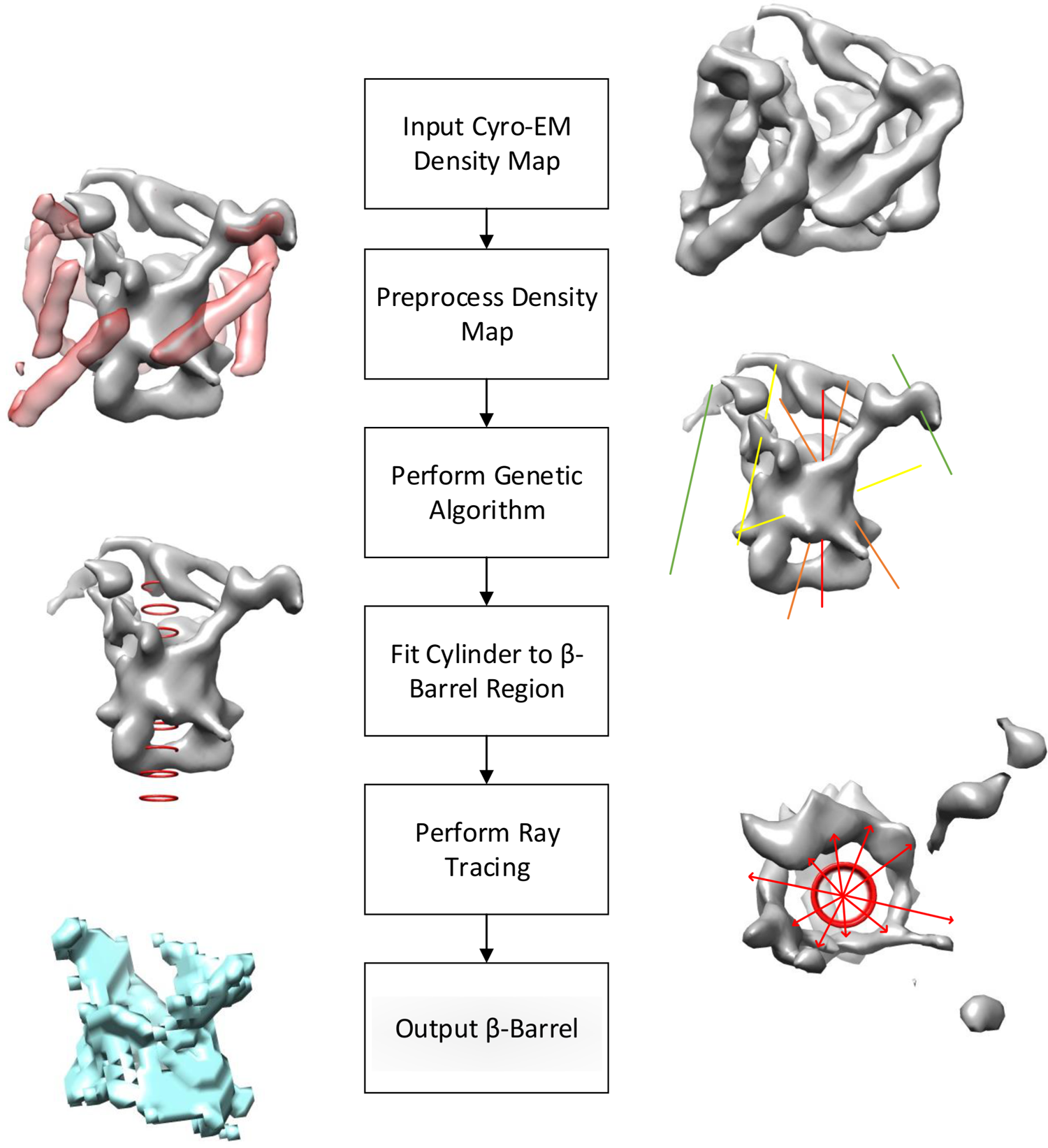
Figure 2 lists out the major steps that are involved in our method.
Flowchart of the major steps in the method.
2.1. Preprocessing
The purpose of preprocessing is to remove unnecessary voxels from within the cryo-EM density map. This is done to increase the effectiveness of the genetic algorithm search by removing background and non-\documentclass{aastex}\usepackage{amsbsy}\usepackage{amsfonts}\usepackage{amssymb}\usepackage{bm}\usepackage{mathrsfs}\usepackage{pifont}\usepackage{stmaryrd}\usepackage{textcomp}\usepackage{portland, xspace}\usepackage{amsmath, amsxtra}\usepackage{upgreek}\pagestyle{empty}\DeclareMathSizes{10}{9}{7}{6}\begin{document}
$$\beta$$
\end{document}-barrel voxels. Furthermore, by removing the total number of voxels needed to perform computations for, the performance of this method increases.
2.1.1. Thresholding
A global minimum density threshold is set for the entire cryo-EM density map and all voxels with a lower density than the selected threshold are removed from the density map as background noise voxels. This is done by loading the density maps into Chimera (Pettersen et al., 2004), where a global threshold is manually selected where most of the background noise voxels are eliminated while retaining the \documentclass{aastex}\usepackage{amsbsy}\usepackage{amsfonts}\usepackage{amssymb}\usepackage{bm}\usepackage{mathrsfs}\usepackage{pifont}\usepackage{stmaryrd}\usepackage{textcomp}\usepackage{portland, xspace}\usepackage{amsmath, amsxtra}\usepackage{upgreek}\pagestyle{empty}\DeclareMathSizes{10}{9}{7}{6}\begin{document}
$$\beta$$
\end{document}-barrel.
2.1.2. Removal of \documentclass{aastex}\usepackage{amsbsy}\usepackage{amsfonts}\usepackage{amssymb}\usepackage{bm}\usepackage{mathrsfs}\usepackage{pifont}\usepackage{stmaryrd}\usepackage{textcomp}\usepackage{portland, xspace}\usepackage{amsmath, amsxtra}\usepackage{upgreek}\pagestyle{empty}\DeclareMathSizes{10}{9}{7}{6}\begin{document}
$$\alpha$$
\end{document}-helices
The \documentclass{aastex}\usepackage{amsbsy}\usepackage{amsfonts}\usepackage{amssymb}\usepackage{bm}\usepackage{mathrsfs}\usepackage{pifont}\usepackage{stmaryrd}\usepackage{textcomp}\usepackage{portland, xspace}\usepackage{amsmath, amsxtra}\usepackage{upgreek}\pagestyle{empty}\DeclareMathSizes{10}{9}{7}{6}\begin{document}
$$\alpha$$
\end{document}-helices are removed from the density map as non-\documentclass{aastex}\usepackage{amsbsy}\usepackage{amsfonts}\usepackage{amssymb}\usepackage{bm}\usepackage{mathrsfs}\usepackage{pifont}\usepackage{stmaryrd}\usepackage{textcomp}\usepackage{portland, xspace}\usepackage{amsmath, amsxtra}\usepackage{upgreek}\pagestyle{empty}\DeclareMathSizes{10}{9}{7}{6}\begin{document}
$$\beta$$
\end{document}-barrel noise voxels. This is done using Gorgon (Baker et al., 2012) and SSETracer (Si et al., 2012). Using SSETracer to detect \documentclass{aastex}\usepackage{amsbsy}\usepackage{amsfonts}\usepackage{amssymb}\usepackage{bm}\usepackage{mathrsfs}\usepackage{pifont}\usepackage{stmaryrd}\usepackage{textcomp}\usepackage{portland, xspace}\usepackage{amsmath, amsxtra}\usepackage{upgreek}\pagestyle{empty}\DeclareMathSizes{10}{9}{7}{6}\begin{document}
$$\alpha$$
\end{document}-helices from the density map, all voxels within 2.0 Å away from a detected \documentclass{aastex}\usepackage{amsbsy}\usepackage{amsfonts}\usepackage{amssymb}\usepackage{bm}\usepackage{mathrsfs}\usepackage{pifont}\usepackage{stmaryrd}\usepackage{textcomp}\usepackage{portland, xspace}\usepackage{amsmath, amsxtra}\usepackage{upgreek}\pagestyle{empty}\DeclareMathSizes{10}{9}{7}{6}\begin{document}
$$\alpha$$
\end{document}-helix are removed from the density map.
2.1.3. Clustering
The remaining voxels are then clustered into separate small groups of voxels. This is done to further reduce noise voxels and also to allow for the detection of multiple \documentclass{aastex}\usepackage{amsbsy}\usepackage{amsfonts}\usepackage{amssymb}\usepackage{bm}\usepackage{mathrsfs}\usepackage{pifont}\usepackage{stmaryrd}\usepackage{textcomp}\usepackage{portland, xspace}\usepackage{amsmath, amsxtra}\usepackage{upgreek}\pagestyle{empty}\DeclareMathSizes{10}{9}{7}{6}\begin{document}
$$\beta$$
\end{document}-barrels within a single cryo-EM density map.
This is done by utilizing a second manually selected threshold. This is chosen such that \documentclass{aastex}\usepackage{amsbsy}\usepackage{amsfonts}\usepackage{amssymb}\usepackage{bm}\usepackage{mathrsfs}\usepackage{pifont}\usepackage{stmaryrd}\usepackage{textcomp}\usepackage{portland, xspace}\usepackage{amsmath, amsxtra}\usepackage{upgreek}\pagestyle{empty}\DeclareMathSizes{10}{9}{7}{6}\begin{document}
$$\beta$$
\end{document}-barrels within the density map are separated from each other. The voxels not filtered out by this second threshold are grouped into clusters, so that each group is at least 2.0 Å from any other cluster. Finally, for each cluster, any voxel, from the set of voxels produced in the first thresholding step, that is within 2.0 Å of it is also added to the cluster.
Once this is completed, all clusters that have a population less than a predefined threshold are removed from the density map as noise. If there are two or more clusters remaining, then the next steps are applied to each cluster individually one at a time.
2.2. Genetic algorithm
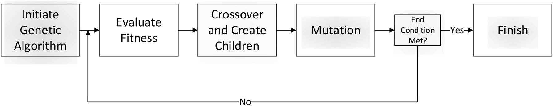
In this method (Fig. 3), the genetic algorithm is used to fit a cylinder into the \documentclass{aastex}\usepackage{amsbsy}\usepackage{amsfonts}\usepackage{amssymb}\usepackage{bm}\usepackage{mathrsfs}\usepackage{pifont}\usepackage{stmaryrd}\usepackage{textcomp}\usepackage{portland, xspace}\usepackage{amsmath, amsxtra}\usepackage{upgreek}\pagestyle{empty}\DeclareMathSizes{10}{9}{7}{6}\begin{document}
$$\beta$$
\end{document}-barrel regions of each cluster(s) within the density map. This cylinder will later be used in the post-processing step to detect the true shape of the \documentclass{aastex}\usepackage{amsbsy}\usepackage{amsfonts}\usepackage{amssymb}\usepackage{bm}\usepackage{mathrsfs}\usepackage{pifont}\usepackage{stmaryrd}\usepackage{textcomp}\usepackage{portland, xspace}\usepackage{amsmath, amsxtra}\usepackage{upgreek}\pagestyle{empty}\DeclareMathSizes{10}{9}{7}{6}\begin{document}
$$\beta$$
\end{document}-barrel.
Flowchart of the steps in the genetic algorithm.
Each candidate in the genetic algorithm is an ideal cylinder that is open at the ends. Each ideal cylinder is defined by a one by seven vector containing seven parameters, [x1, y1, z1, x2, y2, z2, r], representing the center of the two circles that define the two ends of the cylinder and the radius of the cylinder. The genetic algorithm attempts to fit these ideal cylinders so that it aligns with the \documentclass{aastex}\usepackage{amsbsy}\usepackage{amsfonts}\usepackage{amssymb}\usepackage{bm}\usepackage{mathrsfs}\usepackage{pifont}\usepackage{stmaryrd}\usepackage{textcomp}\usepackage{portland, xspace}\usepackage{amsmath, amsxtra}\usepackage{upgreek}\pagestyle{empty}\DeclareMathSizes{10}{9}{7}{6}\begin{document}
$$\beta$$
\end{document}-barrel regions within the density map. In addition, the fitted cylinders should fit completely inside of the \documentclass{aastex}\usepackage{amsbsy}\usepackage{amsfonts}\usepackage{amssymb}\usepackage{bm}\usepackage{mathrsfs}\usepackage{pifont}\usepackage{stmaryrd}\usepackage{textcomp}\usepackage{portland, xspace}\usepackage{amsmath, amsxtra}\usepackage{upgreek}\pagestyle{empty}\DeclareMathSizes{10}{9}{7}{6}\begin{document}
$$\beta$$
\end{document}-barrel region and not touch the walls of the \documentclass{aastex}\usepackage{amsbsy}\usepackage{amsfonts}\usepackage{amssymb}\usepackage{bm}\usepackage{mathrsfs}\usepackage{pifont}\usepackage{stmaryrd}\usepackage{textcomp}\usepackage{portland, xspace}\usepackage{amsmath, amsxtra}\usepackage{upgreek}\pagestyle{empty}\DeclareMathSizes{10}{9}{7}{6}\begin{document}
$$\beta$$
\end{document}-barrel.
An initial population of cylinder candidates is randomly generated at the beginning of the genetic algorithm. Two random 3D points are selected from within a bounding box containing the cluster to act as the two ends of the cylinder. A radius, between 3 and 10 Å, is randomly chosen. For our tests, 200 cylinder candidates were chosen as the population size. The end condition for the genetic algorithm was to run it for 100 generations each time.
The crossover function used in this method pairs up the most fit half of the population in order of their fitness to serve as the “parents” for the next generation. Each parent pairing produces two children cylinder candidates, where each child is given a cylindrical end-point from each parent and its radius is the average of its parents. The mutation step is performed in this method by assigning a chance that each child cylinder has one of its three parameters changed by a mutation factor. This mutation factor follows a nonuniform mutation strategy, so that it is large in earlier generations and decreases as the genetic algorithm is run (Zhao et al., 2007).
2.2.1. Fitness score
Each cylinder candidate has a fitness score that quantifies how likely the cylinder candidate has fit to the \documentclass{aastex}\usepackage{amsbsy}\usepackage{amsfonts}\usepackage{amssymb}\usepackage{bm}\usepackage{mathrsfs}\usepackage{pifont}\usepackage{stmaryrd}\usepackage{textcomp}\usepackage{portland, xspace}\usepackage{amsmath, amsxtra}\usepackage{upgreek}\pagestyle{empty}\DeclareMathSizes{10}{9}{7}{6}\begin{document}
$$\beta$$
\end{document}-barrel region of a cluster. The lower the fitness score, the more likely the cylinder has fitted to the \documentclass{aastex}\usepackage{amsbsy}\usepackage{amsfonts}\usepackage{amssymb}\usepackage{bm}\usepackage{mathrsfs}\usepackage{pifont}\usepackage{stmaryrd}\usepackage{textcomp}\usepackage{portland, xspace}\usepackage{amsmath, amsxtra}\usepackage{upgreek}\pagestyle{empty}\DeclareMathSizes{10}{9}{7}{6}\begin{document}
$$\beta$$
\end{document}-barrel. The fitness score, F, is given by
\documentclass{aastex}\usepackage{amsbsy}\usepackage{amsfonts}\usepackage{amssymb}\usepackage{bm}\usepackage{mathrsfs}\usepackage{pifont}\usepackage{stmaryrd}\usepackage{textcomp}\usepackage{portland, xspace}\usepackage{amsmath, amsxtra}\usepackage{upgreek}\pagestyle{empty}\DeclareMathSizes{10}{9}{7}{6}\begin{document}
\begin{align*}
F = MSE + BP. \tag{1}
\end{align*}
\end{document}
The mean-squared error (MSE) is calculated by
\documentclass{aastex}\usepackage{amsbsy}\usepackage{amsfonts}\usepackage{amssymb}\usepackage{bm}\usepackage{mathrsfs}\usepackage{pifont}\usepackage{stmaryrd}\usepackage{textcomp}\usepackage{portland, xspace}\usepackage{amsmath, amsxtra}\usepackage{upgreek}\pagestyle{empty}\DeclareMathSizes{10}{9}{7}{6}\begin{document}
\begin{align*}
MSE = \mathop \sum \limits_i^N { ( {d_i} ) ^2} / N , \tag{2}
\end{align*}
\end{document}
where N is the number of voxels in the cluster and di is the shortest distance between the i-th voxel in the density map and the surface of the cylinder.
The Barrel Penalty (BP) is a penalty for when voxels are located inside of the cylinder candidate. As a \documentclass{aastex}\usepackage{amsbsy}\usepackage{amsfonts}\usepackage{amssymb}\usepackage{bm}\usepackage{mathrsfs}\usepackage{pifont}\usepackage{stmaryrd}\usepackage{textcomp}\usepackage{portland, xspace}\usepackage{amsmath, amsxtra}\usepackage{upgreek}\pagestyle{empty}\DeclareMathSizes{10}{9}{7}{6}\begin{document}
$$\beta$$
\end{document}-barrel should be hollow inside, there should not be any voxels inside and the BP is a way to bias the genetic algorithm so that it fits cylinders inside the \documentclass{aastex}\usepackage{amsbsy}\usepackage{amsfonts}\usepackage{amssymb}\usepackage{bm}\usepackage{mathrsfs}\usepackage{pifont}\usepackage{stmaryrd}\usepackage{textcomp}\usepackage{portland, xspace}\usepackage{amsmath, amsxtra}\usepackage{upgreek}\pagestyle{empty}\DeclareMathSizes{10}{9}{7}{6}\begin{document}
$$\beta$$
\end{document}-barrel. The BP is calculated by
\documentclass{aastex}\usepackage{amsbsy}\usepackage{amsfonts}\usepackage{amssymb}\usepackage{bm}\usepackage{mathrsfs}\usepackage{pifont}\usepackage{stmaryrd}\usepackage{textcomp}\usepackage{portland, xspace}\usepackage{amsmath, amsxtra}\usepackage{upgreek}\pagestyle{empty}\DeclareMathSizes{10}{9}{7}{6}\begin{document}
\begin{align*}
BP = \mathop \sum \limits_j^M { ( {d_j} ) ^3} , \tag{3}
\end{align*}
\end{document}
where M is the number of voxels located inside the cylinder and dj is the shortest distance between the j-th voxel inside of the cylinder and the surface of the cylinder.
2.3. Postprocessing
Using the cylinder(s) found by the genetic algorithm step already mentioned, the postprocessing step seeks to use the cylinders to isolate and detect the true shape of the \documentclass{aastex}\usepackage{amsbsy}\usepackage{amsfonts}\usepackage{amssymb}\usepackage{bm}\usepackage{mathrsfs}\usepackage{pifont}\usepackage{stmaryrd}\usepackage{textcomp}\usepackage{portland, xspace}\usepackage{amsmath, amsxtra}\usepackage{upgreek}\pagestyle{empty}\DeclareMathSizes{10}{9}{7}{6}\begin{document}
$$\beta$$
\end{document}-barrel through ray tracing.
2.3.1. kd-Tree
The first step in postprocessing is to produce a kd-tree for each cluster. A kd-tree is a binary search tree that is used to recursively partition a space (Bentley, 1975). Every node in the kd-tree represents a subsection of the entire space. The entire space is recursively divided until every leaf contains at most a predefined maximum number of voxels within its subsection. The purpose of the kd-tree is to reduce the number of computations necessary to perform ray tracing in the next step (Wald and Havran, 2006). Instead of checking with every single voxel in the set as in regular ray tracing, every ray can first check whether it passes through the subsection in the first place, before checking with every voxel in that subsection.
2.3.2. Ray tracing
Because the shape of \documentclass{aastex}\usepackage{amsbsy}\usepackage{amsfonts}\usepackage{amssymb}\usepackage{bm}\usepackage{mathrsfs}\usepackage{pifont}\usepackage{stmaryrd}\usepackage{textcomp}\usepackage{portland, xspace}\usepackage{amsmath, amsxtra}\usepackage{upgreek}\pagestyle{empty}\DeclareMathSizes{10}{9}{7}{6}\begin{document}
$$\beta$$
\end{document}-barrels can vary greatly, it is difficult to find a single regular shape that can accurately represent the true shape of a \documentclass{aastex}\usepackage{amsbsy}\usepackage{amsfonts}\usepackage{amssymb}\usepackage{bm}\usepackage{mathrsfs}\usepackage{pifont}\usepackage{stmaryrd}\usepackage{textcomp}\usepackage{portland, xspace}\usepackage{amsmath, amsxtra}\usepackage{upgreek}\pagestyle{empty}\DeclareMathSizes{10}{9}{7}{6}\begin{document}
$$\beta$$
\end{document}-barrel. This method attempts to avoid this problem by utilizing ray tracing to obtain the true shape of a \documentclass{aastex}\usepackage{amsbsy}\usepackage{amsfonts}\usepackage{amssymb}\usepackage{bm}\usepackage{mathrsfs}\usepackage{pifont}\usepackage{stmaryrd}\usepackage{textcomp}\usepackage{portland, xspace}\usepackage{amsmath, amsxtra}\usepackage{upgreek}\pagestyle{empty}\DeclareMathSizes{10}{9}{7}{6}\begin{document}
$$\beta$$
\end{document}-barrel instead. Ray tracing is a computer graphics technique that mimics how light rays work in the real world (Goldstein and Nagel, 1971). By utilizing the fitted cylinders from the genetic algorithm, we shoot rays around the cylinder to identify the voxels that make up the walls of the \documentclass{aastex}\usepackage{amsbsy}\usepackage{amsfonts}\usepackage{amssymb}\usepackage{bm}\usepackage{mathrsfs}\usepackage{pifont}\usepackage{stmaryrd}\usepackage{textcomp}\usepackage{portland, xspace}\usepackage{amsmath, amsxtra}\usepackage{upgreek}\pagestyle{empty}\DeclareMathSizes{10}{9}{7}{6}\begin{document}
$$\beta$$
\end{document}-barrel. This allows us to obtain a more accurate representation of the \documentclass{aastex}\usepackage{amsbsy}\usepackage{amsfonts}\usepackage{amssymb}\usepackage{bm}\usepackage{mathrsfs}\usepackage{pifont}\usepackage{stmaryrd}\usepackage{textcomp}\usepackage{portland, xspace}\usepackage{amsmath, amsxtra}\usepackage{upgreek}\pagestyle{empty}\DeclareMathSizes{10}{9}{7}{6}\begin{document}
$$\beta$$
\end{document}-barrels.
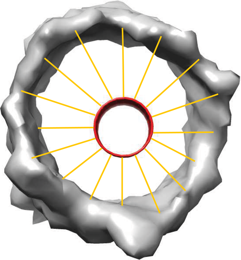
This is done by splitting up the fitted cylinders into evenly divided circular slices. For each slice, rays are shot out, every \documentclass{aastex}\usepackage{amsbsy}\usepackage{amsfonts}\usepackage{amssymb}\usepackage{bm}\usepackage{mathrsfs}\usepackage{pifont}\usepackage{stmaryrd}\usepackage{textcomp}\usepackage{portland, xspace}\usepackage{amsmath, amsxtra}\usepackage{upgreek}\pagestyle{empty}\DeclareMathSizes{10}{9}{7}{6}\begin{document}
$${1^ \circ }$$
\end{document}, from the center of the slice out toward the edges of the slice (Fig. 4). For each ray that is shot out, all voxels within 0.5 Å of the casted ray are added as potential collision candidates. If no voxels meet this requirement, then it is assumed that the ray was shot into empty space. For all of the potential collision candidates, the scalar projection of the voxel candidate onto the casted ray is calculated. Voxels with negative scalar projections are removed as these voxels are “behind” the ray. Finally, the voxel with the smallest scalar projection is chosen as the voxel that the ray intersected with.
Ray tracing for a single slice of the fitted cylinder. The red cylinder in the center is the fitted cylinder. The orange lines represent the rays being casted from the cylinder.
2.3.3. Extending and shrinking the cylinder
The ratio of rays that intersected with a voxel over the total number of rays casted is determined for every single slice. Starting from the two outside slices, the slice (and associated voxels) is removed if it does not achieve at least a ratio of 0.6. This process continues until a slice with at least a ratio of 0.6 is reached. If all of the slices are removed, then this would suggest that there is no \documentclass{aastex}\usepackage{amsbsy}\usepackage{amsfonts}\usepackage{amssymb}\usepackage{bm}\usepackage{mathrsfs}\usepackage{pifont}\usepackage{stmaryrd}\usepackage{textcomp}\usepackage{portland, xspace}\usepackage{amsmath, amsxtra}\usepackage{upgreek}\pagestyle{empty}\DeclareMathSizes{10}{9}{7}{6}\begin{document}
$$\beta$$
\end{document}-barrel in the cluster. This is done because the fitted cylinder is generally longer than the actual \documentclass{aastex}\usepackage{amsbsy}\usepackage{amsfonts}\usepackage{amssymb}\usepackage{bm}\usepackage{mathrsfs}\usepackage{pifont}\usepackage{stmaryrd}\usepackage{textcomp}\usepackage{portland, xspace}\usepackage{amsmath, amsxtra}\usepackage{upgreek}\pagestyle{empty}\DeclareMathSizes{10}{9}{7}{6}\begin{document}
$$\beta$$
\end{document}-barrel and this process removes the non-\documentclass{aastex}\usepackage{amsbsy}\usepackage{amsfonts}\usepackage{amssymb}\usepackage{bm}\usepackage{mathrsfs}\usepackage{pifont}\usepackage{stmaryrd}\usepackage{textcomp}\usepackage{portland, xspace}\usepackage{amsmath, amsxtra}\usepackage{upgreek}\pagestyle{empty}\DeclareMathSizes{10}{9}{7}{6}\begin{document}
$$\beta$$
\end{document}-barrel voxels commonly found at the edge of the \documentclass{aastex}\usepackage{amsbsy}\usepackage{amsfonts}\usepackage{amssymb}\usepackage{bm}\usepackage{mathrsfs}\usepackage{pifont}\usepackage{stmaryrd}\usepackage{textcomp}\usepackage{portland, xspace}\usepackage{amsmath, amsxtra}\usepackage{upgreek}\pagestyle{empty}\DeclareMathSizes{10}{9}{7}{6}\begin{document}
$$\beta$$
\end{document}-barrel.
Conversely, if one of the two (or both) edge slices achieve at least a 0.6 ratio, then an additional slice is added to the end of the cylinder and ray tracing is performed for that slice. If the added slice achieves at least a 0.6 ratio as well, then it is added as part of the \documentclass{aastex}\usepackage{amsbsy}\usepackage{amsfonts}\usepackage{amssymb}\usepackage{bm}\usepackage{mathrsfs}\usepackage{pifont}\usepackage{stmaryrd}\usepackage{textcomp}\usepackage{portland, xspace}\usepackage{amsmath, amsxtra}\usepackage{upgreek}\pagestyle{empty}\DeclareMathSizes{10}{9}{7}{6}\begin{document}
$$\beta$$
\end{document}-barrel and additional slices are added continuously until an added slice does not achieve at least a 0.6 ratio. This was added to account for the case in which the genetic algorithm may fit a cylinder that is shorter than the actual \documentclass{aastex}\usepackage{amsbsy}\usepackage{amsfonts}\usepackage{amssymb}\usepackage{bm}\usepackage{mathrsfs}\usepackage{pifont}\usepackage{stmaryrd}\usepackage{textcomp}\usepackage{portland, xspace}\usepackage{amsmath, amsxtra}\usepackage{upgreek}\pagestyle{empty}\DeclareMathSizes{10}{9}{7}{6}\begin{document}
$$\beta$$
\end{document}-barrel.
2.3.4. Removal of outlier voxels
The last step in postprocessing involves removing outlier voxels. As there may be gaps in the \documentclass{aastex}\usepackage{amsbsy}\usepackage{amsfonts}\usepackage{amssymb}\usepackage{bm}\usepackage{mathrsfs}\usepackage{pifont}\usepackage{stmaryrd}\usepackage{textcomp}\usepackage{portland, xspace}\usepackage{amsmath, amsxtra}\usepackage{upgreek}\pagestyle{empty}\DeclareMathSizes{10}{9}{7}{6}\begin{document}
$$\beta$$
\end{document}-barrel wall, rays may shoot through these gaps and intersect with voxels that are far away from the \documentclass{aastex}\usepackage{amsbsy}\usepackage{amsfonts}\usepackage{amssymb}\usepackage{bm}\usepackage{mathrsfs}\usepackage{pifont}\usepackage{stmaryrd}\usepackage{textcomp}\usepackage{portland, xspace}\usepackage{amsmath, amsxtra}\usepackage{upgreek}\pagestyle{empty}\DeclareMathSizes{10}{9}{7}{6}\begin{document}
$$\beta$$
\end{document}-barrel. How this possibility was accounted for was to remove all voxels that are more than 2\documentclass{aastex}\usepackage{amsbsy}\usepackage{amsfonts}\usepackage{amssymb}\usepackage{bm}\usepackage{mathrsfs}\usepackage{pifont}\usepackage{stmaryrd}\usepackage{textcomp}\usepackage{portland, xspace}\usepackage{amsmath, amsxtra}\usepackage{upgreek}\pagestyle{empty}\DeclareMathSizes{10}{9}{7}{6}\begin{document}
$$\sigma$$
\end{document} away from the mean distance between the cylinder and the intersected voxels.
2.4. Metrics
Our method used two metrics to quantify the accuracy of detection, sensitivity, and specificity (Altman and Bland, 1994). These two metrics are calculated based on \documentclass{aastex}\usepackage{amsbsy}\usepackage{amsfonts}\usepackage{amssymb}\usepackage{bm}\usepackage{mathrsfs}\usepackage{pifont}\usepackage{stmaryrd}\usepackage{textcomp}\usepackage{portland, xspace}\usepackage{amsmath, amsxtra}\usepackage{upgreek}\pagestyle{empty}\DeclareMathSizes{10}{9}{7}{6}\begin{document}
$${\rm C} \alpha$$
\end{document} (or \documentclass{aastex}\usepackage{amsbsy}\usepackage{amsfonts}\usepackage{amssymb}\usepackage{bm}\usepackage{mathrsfs}\usepackage{pifont}\usepackage{stmaryrd}\usepackage{textcomp}\usepackage{portland, xspace}\usepackage{amsmath, amsxtra}\usepackage{upgreek}\pagestyle{empty}\DeclareMathSizes{10}{9}{7}{6}\begin{document}
$$\alpha$$
\end{document} carbon) in the proteins tested. A \documentclass{aastex}\usepackage{amsbsy}\usepackage{amsfonts}\usepackage{amssymb}\usepackage{bm}\usepackage{mathrsfs}\usepackage{pifont}\usepackage{stmaryrd}\usepackage{textcomp}\usepackage{portland, xspace}\usepackage{amsmath, amsxtra}\usepackage{upgreek}\pagestyle{empty}\DeclareMathSizes{10}{9}{7}{6}\begin{document}
$$\alpha$$
\end{document} carbon is the carbon atom on the backbone that is attached to the side chain in each amino acid. A \documentclass{aastex}\usepackage{amsbsy}\usepackage{amsfonts}\usepackage{amssymb}\usepackage{bm}\usepackage{mathrsfs}\usepackage{pifont}\usepackage{stmaryrd}\usepackage{textcomp}\usepackage{portland, xspace}\usepackage{amsmath, amsxtra}\usepackage{upgreek}\pagestyle{empty}\DeclareMathSizes{10}{9}{7}{6}\begin{document}
$${\rm C} \alpha$$
\end{document} is declared detected if there are detected voxels that are within 2.0 Å from it.
Sensitivity indicates the percentage of \documentclass{aastex}\usepackage{amsbsy}\usepackage{amsfonts}\usepackage{amssymb}\usepackage{bm}\usepackage{mathrsfs}\usepackage{pifont}\usepackage{stmaryrd}\usepackage{textcomp}\usepackage{portland, xspace}\usepackage{amsmath, amsxtra}\usepackage{upgreek}\pagestyle{empty}\DeclareMathSizes{10}{9}{7}{6}\begin{document}
$$\beta$$
\end{document}-barrel \documentclass{aastex}\usepackage{amsbsy}\usepackage{amsfonts}\usepackage{amssymb}\usepackage{bm}\usepackage{mathrsfs}\usepackage{pifont}\usepackage{stmaryrd}\usepackage{textcomp}\usepackage{portland, xspace}\usepackage{amsmath, amsxtra}\usepackage{upgreek}\pagestyle{empty}\DeclareMathSizes{10}{9}{7}{6}\begin{document}
$${\rm C} \alpha$$
\end{document} correctly detected (true positive). This is calculated by
\documentclass{aastex}\usepackage{amsbsy}\usepackage{amsfonts}\usepackage{amssymb}\usepackage{bm}\usepackage{mathrsfs}\usepackage{pifont}\usepackage{stmaryrd}\usepackage{textcomp}\usepackage{portland, xspace}\usepackage{amsmath, amsxtra}\usepackage{upgreek}\pagestyle{empty}\DeclareMathSizes{10}{9}{7}{6}\begin{document}
\begin{align*}
\begin{matrix} {Sensitivity = No \ of \beta { \rm{ - }}barrel \ C \alpha \ detected / } \hfill \\ { \quad \quad \quad total \ No \ of \beta { \rm{ - }}barrel \ C \alpha \ in \ protein} \hfill \\ \end{matrix}. \tag{4}
\end{align*}
\end{document}
Specificity represents the percentage of non-\documentclass{aastex}\usepackage{amsbsy}\usepackage{amsfonts}\usepackage{amssymb}\usepackage{bm}\usepackage{mathrsfs}\usepackage{pifont}\usepackage{stmaryrd}\usepackage{textcomp}\usepackage{portland, xspace}\usepackage{amsmath, amsxtra}\usepackage{upgreek}\pagestyle{empty}\DeclareMathSizes{10}{9}{7}{6}\begin{document}
$$\beta$$
\end{document}-barrel \documentclass{aastex}\usepackage{amsbsy}\usepackage{amsfonts}\usepackage{amssymb}\usepackage{bm}\usepackage{mathrsfs}\usepackage{pifont}\usepackage{stmaryrd}\usepackage{textcomp}\usepackage{portland, xspace}\usepackage{amsmath, amsxtra}\usepackage{upgreek}\pagestyle{empty}\DeclareMathSizes{10}{9}{7}{6}\begin{document}
$${\rm C} \alpha$$
\end{document} correctly detected as non-\documentclass{aastex}\usepackage{amsbsy}\usepackage{amsfonts}\usepackage{amssymb}\usepackage{bm}\usepackage{mathrsfs}\usepackage{pifont}\usepackage{stmaryrd}\usepackage{textcomp}\usepackage{portland, xspace}\usepackage{amsmath, amsxtra}\usepackage{upgreek}\pagestyle{empty}\DeclareMathSizes{10}{9}{7}{6}\begin{document}
$$\beta$$
\end{document}-barrel \documentclass{aastex}\usepackage{amsbsy}\usepackage{amsfonts}\usepackage{amssymb}\usepackage{bm}\usepackage{mathrsfs}\usepackage{pifont}\usepackage{stmaryrd}\usepackage{textcomp}\usepackage{portland, xspace}\usepackage{amsmath, amsxtra}\usepackage{upgreek}\pagestyle{empty}\DeclareMathSizes{10}{9}{7}{6}\begin{document}
$${\rm C} \alpha$$
\end{document}. It is calculated by
\documentclass{aastex}\usepackage{amsbsy}\usepackage{amsfonts}\usepackage{amssymb}\usepackage{bm}\usepackage{mathrsfs}\usepackage{pifont}\usepackage{stmaryrd}\usepackage{textcomp}\usepackage{portland, xspace}\usepackage{amsmath, amsxtra}\usepackage{upgreek}\pagestyle{empty}\DeclareMathSizes{10}{9}{7}{6}\begin{document}
\begin{align*}
\begin{matrix} {Specificity = No \ of \ non{ \rm{ - }} \beta { \rm{ - }}barrel \ C \alpha \ detected / } \hfill \\ { \quad \quad \quad total \ No \ of \ non{ \rm{ - }} \beta { \rm{ - }}barrel \ C \alpha \ in \ protein} \hfill \\ \end{matrix} \tag{5}
\end{align*}
\end{document}
3. Results
3.1. Simulated density maps
Twelve simulated density maps were tested using this method. Using the protein data bank (PDB) file and the EMAN program pdb2mrc (Ludtke et al., 1999), all simulated density maps were generated at a resolution of 9 Å and sampling of 1 Å per pixel. These proteins and PDBs were taken from the CATH database (www.cathdb.info/) under the “Beta Barrel” section.
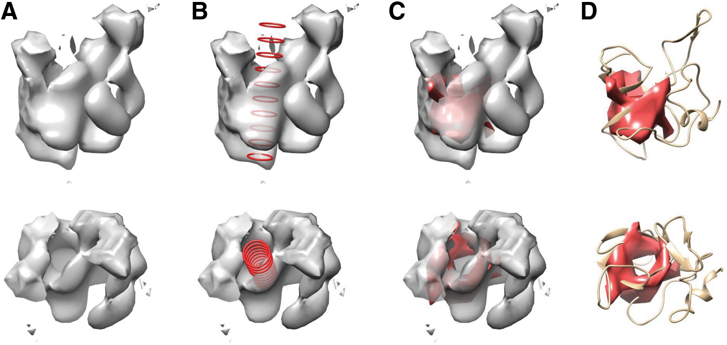
In Figure 5, an example of one of the simulated density maps, protein 1AJZ chain A, tested is shown. The \documentclass{aastex}\usepackage{amsbsy}\usepackage{amsfonts}\usepackage{amssymb}\usepackage{bm}\usepackage{mathrsfs}\usepackage{pifont}\usepackage{stmaryrd}\usepackage{textcomp}\usepackage{portland, xspace}\usepackage{amsmath, amsxtra}\usepackage{upgreek}\pagestyle{empty}\DeclareMathSizes{10}{9}{7}{6}\begin{document}
$$\beta$$
\end{document}-barrel is completely detected using our method for this protein. However, non-\documentclass{aastex}\usepackage{amsbsy}\usepackage{amsfonts}\usepackage{amssymb}\usepackage{bm}\usepackage{mathrsfs}\usepackage{pifont}\usepackage{stmaryrd}\usepackage{textcomp}\usepackage{portland, xspace}\usepackage{amsmath, amsxtra}\usepackage{upgreek}\pagestyle{empty}\DeclareMathSizes{10}{9}{7}{6}\begin{document}
$$\beta$$
\end{document}-barrel density is detected (specificity of 80.0%) because there is density at the ends of the \documentclass{aastex}\usepackage{amsbsy}\usepackage{amsfonts}\usepackage{amssymb}\usepackage{bm}\usepackage{mathrsfs}\usepackage{pifont}\usepackage{stmaryrd}\usepackage{textcomp}\usepackage{portland, xspace}\usepackage{amsmath, amsxtra}\usepackage{upgreek}\pagestyle{empty}\DeclareMathSizes{10}{9}{7}{6}\begin{document}
$$\beta$$
\end{document}-barrel and surrounding the two openings. Because the non-\documentclass{aastex}\usepackage{amsbsy}\usepackage{amsfonts}\usepackage{amssymb}\usepackage{bm}\usepackage{mathrsfs}\usepackage{pifont}\usepackage{stmaryrd}\usepackage{textcomp}\usepackage{portland, xspace}\usepackage{amsmath, amsxtra}\usepackage{upgreek}\pagestyle{empty}\DeclareMathSizes{10}{9}{7}{6}\begin{document}
$$\beta$$
\end{document}-barrel density is somewhat in a ring-like shape, our method cannot distinguish it as not part of the \documentclass{aastex}\usepackage{amsbsy}\usepackage{amsfonts}\usepackage{amssymb}\usepackage{bm}\usepackage{mathrsfs}\usepackage{pifont}\usepackage{stmaryrd}\usepackage{textcomp}\usepackage{portland, xspace}\usepackage{amsmath, amsxtra}\usepackage{upgreek}\pagestyle{empty}\DeclareMathSizes{10}{9}{7}{6}\begin{document}
$$\beta$$
\end{document}-barrel and it is added to the result voxel set.
\documentclass{aastex}\usepackage{amsbsy}\usepackage{amsfonts}\usepackage{amssymb}\usepackage{bm}\usepackage{mathrsfs}\usepackage{pifont}\usepackage{stmaryrd}\usepackage{textcomp}\usepackage{portland, xspace}\usepackage{amsmath, amsxtra}\usepackage{upgreek}\pagestyle{empty}\DeclareMathSizes{10}{9}{7}{6}\begin{document}
$$\beta$$
\end{document}-barrel detection from simulated density maps. (A) Simulated density map of protein 1AJZ chain A at 9 Å resolution. (B) The fitted cylinder (red). (C) The detected \documentclass{aastex}\usepackage{amsbsy}\usepackage{amsfonts}\usepackage{amssymb}\usepackage{bm}\usepackage{mathrsfs}\usepackage{pifont}\usepackage{stmaryrd}\usepackage{textcomp}\usepackage{portland, xspace}\usepackage{amsmath, amsxtra}\usepackage{upgreek}\pagestyle{empty}\DeclareMathSizes{10}{9}{7}{6}\begin{document}
$$\beta$$
\end{document}-barrel surface (red). (D) The detected \documentclass{aastex}\usepackage{amsbsy}\usepackage{amsfonts}\usepackage{amssymb}\usepackage{bm}\usepackage{mathrsfs}\usepackage{pifont}\usepackage{stmaryrd}\usepackage{textcomp}\usepackage{portland, xspace}\usepackage{amsmath, amsxtra}\usepackage{upgreek}\pagestyle{empty}\DeclareMathSizes{10}{9}{7}{6}\begin{document}
$$\beta$$
\end{document}-barrel surface (red) superimposed over the true protein structure.
In Table 1, the results using our method on the 12 simulated density maps are shown. The average sensitivity is 96.6%, which suggests that our method can identify the \documentclass{aastex}\usepackage{amsbsy}\usepackage{amsfonts}\usepackage{amssymb}\usepackage{bm}\usepackage{mathrsfs}\usepackage{pifont}\usepackage{stmaryrd}\usepackage{textcomp}\usepackage{portland, xspace}\usepackage{amsmath, amsxtra}\usepackage{upgreek}\pagestyle{empty}\DeclareMathSizes{10}{9}{7}{6}\begin{document}
$$\beta$$
\end{document}-barrel from within the cryo-EM density map. However, the average specificity of 77.7% suggests that our method struggles at isolating the \documentclass{aastex}\usepackage{amsbsy}\usepackage{amsfonts}\usepackage{amssymb}\usepackage{bm}\usepackage{mathrsfs}\usepackage{pifont}\usepackage{stmaryrd}\usepackage{textcomp}\usepackage{portland, xspace}\usepackage{amsmath, amsxtra}\usepackage{upgreek}\pagestyle{empty}\DeclareMathSizes{10}{9}{7}{6}\begin{document}
$$\beta$$
\end{document}-barrel from the non-\documentclass{aastex}\usepackage{amsbsy}\usepackage{amsfonts}\usepackage{amssymb}\usepackage{bm}\usepackage{mathrsfs}\usepackage{pifont}\usepackage{stmaryrd}\usepackage{textcomp}\usepackage{portland, xspace}\usepackage{amsmath, amsxtra}\usepackage{upgreek}\pagestyle{empty}\DeclareMathSizes{10}{9}{7}{6}\begin{document}
$$\beta$$
\end{document}-barrel voxels from within the density map. This low specificity comes from the areas that are located right at the two ends of the \documentclass{aastex}\usepackage{amsbsy}\usepackage{amsfonts}\usepackage{amssymb}\usepackage{bm}\usepackage{mathrsfs}\usepackage{pifont}\usepackage{stmaryrd}\usepackage{textcomp}\usepackage{portland, xspace}\usepackage{amsmath, amsxtra}\usepackage{upgreek}\pagestyle{empty}\DeclareMathSizes{10}{9}{7}{6}\begin{document}
$$\beta$$
\end{document}-barrel. This density is challenging to isolate and remove from the final result.
Accuracy of \documentclass{aastex}\usepackage{amsbsy}\usepackage{amsfonts}\usepackage{amssymb}\usepackage{bm}\usepackage{mathrsfs}\usepackage{pifont}\usepackage{stmaryrd}\usepackage{textcomp}\usepackage{portland, xspace}\usepackage{amsmath, amsxtra}\usepackage{upgreek}\pagestyle{empty}\DeclareMathSizes{10}{9}{7}{6}\begin{document}
$$\beta$$
\end{document}-Barrel Detection on Simulated Density Maps
PDB ID
Total
Barrel
True positive (TP)
False positive (FP)
Sensitivity
Specificity
1AJZ_A
282
37
37
49
1.000
0.800
1AL7_A
350
34
33
56
0.971
0.823
1JB3_A
127
46
45
10
0.978
0.877
1NNX_A
93
45
45
10
1.000
0.792
1TIM_A
247
50
50
52
1.000
0.736
1HIK_A
136
45
43
23
0.956
0.747
1Y0Y_A
335
35
35
100
1.000
0.667
3GP6_A
166
93
89
25
0.957
0.657
3ULJ_A
96
55
54
7
0.982
0.829
2DYI_A
162
41
38
23
0.927
0.810
2UXW_A
115
47
42
13
0.893
0.809
2F1C_X
252
175
162
17
0.926
0.779
Average
0.966
0.777
3.2. Experimental density maps
Eight experimental density maps were tested using our method. Unlike the simulated density maps, these maps were generated from actual cryo-EM experiments and were obtained from the EM Data Bank (www.emdatabank.org/).
In Figure 6, an example of one of the experimental density maps, EMDB 2605 aligned with protein 4CSU chain K, is shown. For this protein, a high sensitivity (89.3%) and high specificity (92.5%) were obtained using our method.
\documentclass{aastex}\usepackage{amsbsy}\usepackage{amsfonts}\usepackage{amssymb}\usepackage{bm}\usepackage{mathrsfs}\usepackage{pifont}\usepackage{stmaryrd}\usepackage{textcomp}\usepackage{portland, xspace}\usepackage{amsmath, amsxtra}\usepackage{upgreek}\pagestyle{empty}\DeclareMathSizes{10}{9}{7}{6}\begin{document}
$$\beta$$
\end{document}-barrel detection from experimental density maps. (A) Experimental density map of protein 4CSU chain K. (B) The fitted cylinder (red). (C) The detected \documentclass{aastex}\usepackage{amsbsy}\usepackage{amsfonts}\usepackage{amssymb}\usepackage{bm}\usepackage{mathrsfs}\usepackage{pifont}\usepackage{stmaryrd}\usepackage{textcomp}\usepackage{portland, xspace}\usepackage{amsmath, amsxtra}\usepackage{upgreek}\pagestyle{empty}\DeclareMathSizes{10}{9}{7}{6}\begin{document}
$$\beta$$
\end{document}-barrel surface (red). (D) The detected \documentclass{aastex}\usepackage{amsbsy}\usepackage{amsfonts}\usepackage{amssymb}\usepackage{bm}\usepackage{mathrsfs}\usepackage{pifont}\usepackage{stmaryrd}\usepackage{textcomp}\usepackage{portland, xspace}\usepackage{amsmath, amsxtra}\usepackage{upgreek}\pagestyle{empty}\DeclareMathSizes{10}{9}{7}{6}\begin{document}
$$\beta$$
\end{document}-barrel surface (red) superimposed over the true protein structure.
In Table 2, the results of using our method on experimental density maps are shown. The average sensitivity is 81.3%, which is lower than the sensitivity for simulated maps. This suggests that our method is greatly affected by the amount of noise in the density map, as experimental cryo-EM data tend to be incomplete and very noisy.
Accuracy of \documentclass{aastex}\usepackage{amsbsy}\usepackage{amsfonts}\usepackage{amssymb}\usepackage{bm}\usepackage{mathrsfs}\usepackage{pifont}\usepackage{stmaryrd}\usepackage{textcomp}\usepackage{portland, xspace}\usepackage{amsmath, amsxtra}\usepackage{upgreek}\pagestyle{empty}\DeclareMathSizes{10}{9}{7}{6}\begin{document}
$$\beta$$
\end{document}-Barrel Detection on Experimental Density Maps
EMDB PDB ID (Res)
Total
Barrel
True positive (TP)
False positive (FP)
Sensitivity
Specificity
1657_2WWQ_W (5.8 Å)
94
30
23
17
0.767
0.734
1780_3IZ5_M (5.5 Å)
140
28
22
24
0.786
0.786
1849_3IZU_L (8.25 Å)
123
31
24
1
0.774
0.989
1849_3IZU_W (8.25 Å)
94
40
34
9
0.850
0.833
2605_4CSU_K (5.5 Å)
121
28
25
7
0.893
0.925
6396_5A9Z_AL (6.4 Å)
122
30
27
25
0.900
0.728
2169_4 V8T_V (8.1 Å)
136
31
22
11
0.710
0.895
5036_3FIK_K (6.7 Å)
121
29
24
15
0.828
0.837
Average
0.813
0.840
3.3. Density maps with multiple \documentclass{aastex}\usepackage{amsbsy}\usepackage{amsfonts}\usepackage{amssymb}\usepackage{bm}\usepackage{mathrsfs}\usepackage{pifont}\usepackage{stmaryrd}\usepackage{textcomp}\usepackage{portland, xspace}\usepackage{amsmath, amsxtra}\usepackage{upgreek}\pagestyle{empty}\DeclareMathSizes{10}{9}{7}{6}\begin{document}
$$\beta$$
\end{document}-barrels
Three simulated density maps containing multiple \documentclass{aastex}\usepackage{amsbsy}\usepackage{amsfonts}\usepackage{amssymb}\usepackage{bm}\usepackage{mathrsfs}\usepackage{pifont}\usepackage{stmaryrd}\usepackage{textcomp}\usepackage{portland, xspace}\usepackage{amsmath, amsxtra}\usepackage{upgreek}\pagestyle{empty}\DeclareMathSizes{10}{9}{7}{6}\begin{document}
$$\beta$$
\end{document}-barrels were tested using this method. These proteins and their PDBs were found on the RCSB PDB databank (www.rcsb.org).
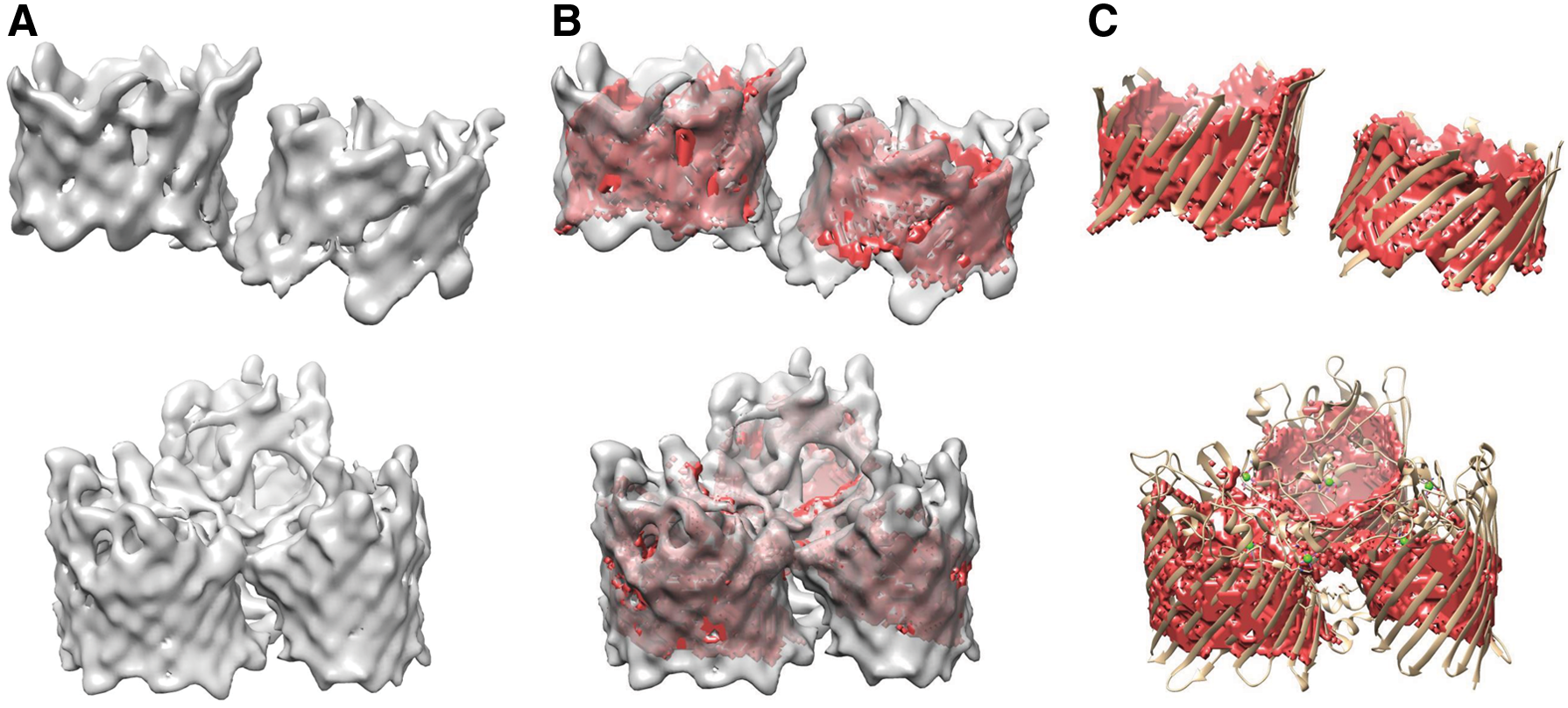
In Figure 7, we demonstrate two examples of density maps with multiple \documentclass{aastex}\usepackage{amsbsy}\usepackage{amsfonts}\usepackage{amssymb}\usepackage{bm}\usepackage{mathrsfs}\usepackage{pifont}\usepackage{stmaryrd}\usepackage{textcomp}\usepackage{portland, xspace}\usepackage{amsmath, amsxtra}\usepackage{upgreek}\pagestyle{empty}\DeclareMathSizes{10}{9}{7}{6}\begin{document}
$$\beta$$
\end{document}-barrels. Protein 5XDO is a very large protein that contains two very clear and very large \documentclass{aastex}\usepackage{amsbsy}\usepackage{amsfonts}\usepackage{amssymb}\usepackage{bm}\usepackage{mathrsfs}\usepackage{pifont}\usepackage{stmaryrd}\usepackage{textcomp}\usepackage{portland, xspace}\usepackage{amsmath, amsxtra}\usepackage{upgreek}\pagestyle{empty}\DeclareMathSizes{10}{9}{7}{6}\begin{document}
$$\beta$$
\end{document}-barrels. Our method was able to accurately detect both barrels, resulting in very high sensitivity and specificity values. Protein 5LDT is also a very large protein that contains three \documentclass{aastex}\usepackage{amsbsy}\usepackage{amsfonts}\usepackage{amssymb}\usepackage{bm}\usepackage{mathrsfs}\usepackage{pifont}\usepackage{stmaryrd}\usepackage{textcomp}\usepackage{portland, xspace}\usepackage{amsmath, amsxtra}\usepackage{upgreek}\pagestyle{empty}\DeclareMathSizes{10}{9}{7}{6}\begin{document}
$$\beta$$
\end{document}-barrels. Unlike 5XDO, the \documentclass{aastex}\usepackage{amsbsy}\usepackage{amsfonts}\usepackage{amssymb}\usepackage{bm}\usepackage{mathrsfs}\usepackage{pifont}\usepackage{stmaryrd}\usepackage{textcomp}\usepackage{portland, xspace}\usepackage{amsmath, amsxtra}\usepackage{upgreek}\pagestyle{empty}\DeclareMathSizes{10}{9}{7}{6}\begin{document}
$$\beta$$
\end{document}-barrel is much less clear and contains density in and around the \documentclass{aastex}\usepackage{amsbsy}\usepackage{amsfonts}\usepackage{amssymb}\usepackage{bm}\usepackage{mathrsfs}\usepackage{pifont}\usepackage{stmaryrd}\usepackage{textcomp}\usepackage{portland, xspace}\usepackage{amsmath, amsxtra}\usepackage{upgreek}\pagestyle{empty}\DeclareMathSizes{10}{9}{7}{6}\begin{document}
$$\beta$$
\end{document}-barrel opening. Although our method was capable of detecting most of the \documentclass{aastex}\usepackage{amsbsy}\usepackage{amsfonts}\usepackage{amssymb}\usepackage{bm}\usepackage{mathrsfs}\usepackage{pifont}\usepackage{stmaryrd}\usepackage{textcomp}\usepackage{portland, xspace}\usepackage{amsmath, amsxtra}\usepackage{upgreek}\pagestyle{empty}\DeclareMathSizes{10}{9}{7}{6}\begin{document}
$$\beta$$
\end{document}-barrel, the additional noise results in a significant drop in accuracy.
\documentclass{aastex}\usepackage{amsbsy}\usepackage{amsfonts}\usepackage{amssymb}\usepackage{bm}\usepackage{mathrsfs}\usepackage{pifont}\usepackage{stmaryrd}\usepackage{textcomp}\usepackage{portland, xspace}\usepackage{amsmath, amsxtra}\usepackage{upgreek}\pagestyle{empty}\DeclareMathSizes{10}{9}{7}{6}\begin{document}
$$\beta$$
\end{document}-barrel detection from density maps with multiple barrels. Top row represents protein 5XDO. Bottom row represents protein 5LDT. (A) Simulated density map of protein 5XDN at 9 Å resolution. (B) The detected \documentclass{aastex}\usepackage{amsbsy}\usepackage{amsfonts}\usepackage{amssymb}\usepackage{bm}\usepackage{mathrsfs}\usepackage{pifont}\usepackage{stmaryrd}\usepackage{textcomp}\usepackage{portland, xspace}\usepackage{amsmath, amsxtra}\usepackage{upgreek}\pagestyle{empty}\DeclareMathSizes{10}{9}{7}{6}\begin{document}
$$\beta$$
\end{document}-barrel surface (red) superimposed over the density map. (C) The detected \documentclass{aastex}\usepackage{amsbsy}\usepackage{amsfonts}\usepackage{amssymb}\usepackage{bm}\usepackage{mathrsfs}\usepackage{pifont}\usepackage{stmaryrd}\usepackage{textcomp}\usepackage{portland, xspace}\usepackage{amsmath, amsxtra}\usepackage{upgreek}\pagestyle{empty}\DeclareMathSizes{10}{9}{7}{6}\begin{document}
$$\beta$$
\end{document}-barrel surface (red) superimposed over the true protein structure.
In Table 3, the results of applying our method on density maps with multiple \documentclass{aastex}\usepackage{amsbsy}\usepackage{amsfonts}\usepackage{amssymb}\usepackage{bm}\usepackage{mathrsfs}\usepackage{pifont}\usepackage{stmaryrd}\usepackage{textcomp}\usepackage{portland, xspace}\usepackage{amsmath, amsxtra}\usepackage{upgreek}\pagestyle{empty}\DeclareMathSizes{10}{9}{7}{6}\begin{document}
$$\beta$$
\end{document}-barrels are shown. For the proteins 5XDN and 5XDO, the \documentclass{aastex}\usepackage{amsbsy}\usepackage{amsfonts}\usepackage{amssymb}\usepackage{bm}\usepackage{mathrsfs}\usepackage{pifont}\usepackage{stmaryrd}\usepackage{textcomp}\usepackage{portland, xspace}\usepackage{amsmath, amsxtra}\usepackage{upgreek}\pagestyle{empty}\DeclareMathSizes{10}{9}{7}{6}\begin{document}
$$\beta$$
\end{document}-barrel is very prominent and there is very little non-\documentclass{aastex}\usepackage{amsbsy}\usepackage{amsfonts}\usepackage{amssymb}\usepackage{bm}\usepackage{mathrsfs}\usepackage{pifont}\usepackage{stmaryrd}\usepackage{textcomp}\usepackage{portland, xspace}\usepackage{amsmath, amsxtra}\usepackage{upgreek}\pagestyle{empty}\DeclareMathSizes{10}{9}{7}{6}\begin{document}
$$\beta$$
\end{document}-barrel density around the barrel openings. This results in very high sensitivities and specificities. In contrast, for protein 5LDT, there exists significant amount of non-\documentclass{aastex}\usepackage{amsbsy}\usepackage{amsfonts}\usepackage{amssymb}\usepackage{bm}\usepackage{mathrsfs}\usepackage{pifont}\usepackage{stmaryrd}\usepackage{textcomp}\usepackage{portland, xspace}\usepackage{amsmath, amsxtra}\usepackage{upgreek}\pagestyle{empty}\DeclareMathSizes{10}{9}{7}{6}\begin{document}
$$\beta$$
\end{document}-barrel densities around and blocking the barrel openings and this results in a significant drop in sensitivity and specificity.
Accuracy of \documentclass{aastex}\usepackage{amsbsy}\usepackage{amsfonts}\usepackage{amssymb}\usepackage{bm}\usepackage{mathrsfs}\usepackage{pifont}\usepackage{stmaryrd}\usepackage{textcomp}\usepackage{portland, xspace}\usepackage{amsmath, amsxtra}\usepackage{upgreek}\pagestyle{empty}\DeclareMathSizes{10}{9}{7}{6}\begin{document}
$$\beta$$
\end{document}-Barrel Detection on Density Maps with Multiple \documentclass{aastex}\usepackage{amsbsy}\usepackage{amsfonts}\usepackage{amssymb}\usepackage{bm}\usepackage{mathrsfs}\usepackage{pifont}\usepackage{stmaryrd}\usepackage{textcomp}\usepackage{portland, xspace}\usepackage{amsmath, amsxtra}\usepackage{upgreek}\pagestyle{empty}\DeclareMathSizes{10}{9}{7}{6}\begin{document}
$$\beta$$
\end{document}-Barrels
PDB ID
Total
Barrel
True positive (TP)
False positive (FP)
Sensitivity
Specificity
Total barrels
Barrels detected
5XDN
550
355
327
8
0.921
0.959
2
2
5XDO
541
336
312
5
0.928
0.975
2
2
5LDT
1212
719
504
158
0.701
0.679
3
3
Average
0.850
0.871
3.4. Density maps with no \documentclass{aastex}\usepackage{amsbsy}\usepackage{amsfonts}\usepackage{amssymb}\usepackage{bm}\usepackage{mathrsfs}\usepackage{pifont}\usepackage{stmaryrd}\usepackage{textcomp}\usepackage{portland, xspace}\usepackage{amsmath, amsxtra}\usepackage{upgreek}\pagestyle{empty}\DeclareMathSizes{10}{9}{7}{6}\begin{document}
$$\beta$$
\end{document}-barrels
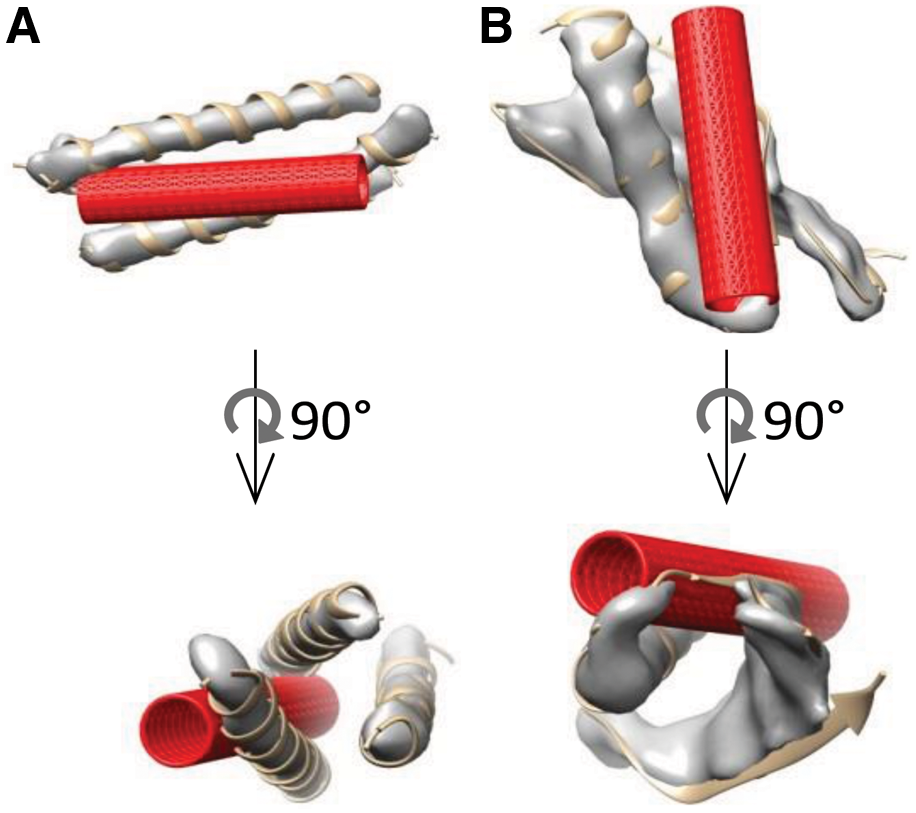
In addition, our method was also tested on density maps that did not contain a \documentclass{aastex}\usepackage{amsbsy}\usepackage{amsfonts}\usepackage{amssymb}\usepackage{bm}\usepackage{mathrsfs}\usepackage{pifont}\usepackage{stmaryrd}\usepackage{textcomp}\usepackage{portland, xspace}\usepackage{amsmath, amsxtra}\usepackage{upgreek}\pagestyle{empty}\DeclareMathSizes{10}{9}{7}{6}\begin{document}
$$\beta$$
\end{document}-barrel. In Figure 8, we demonstrate two proteins that were accurately detected to not contain any \documentclass{aastex}\usepackage{amsbsy}\usepackage{amsfonts}\usepackage{amssymb}\usepackage{bm}\usepackage{mathrsfs}\usepackage{pifont}\usepackage{stmaryrd}\usepackage{textcomp}\usepackage{portland, xspace}\usepackage{amsmath, amsxtra}\usepackage{upgreek}\pagestyle{empty}\DeclareMathSizes{10}{9}{7}{6}\begin{document}
$$\beta$$
\end{document}-barrels within it, PDB 1COS chain A and 4R80 chain A. Therefore, our method accurately identified that the density map did not contain a \documentclass{aastex}\usepackage{amsbsy}\usepackage{amsfonts}\usepackage{amssymb}\usepackage{bm}\usepackage{mathrsfs}\usepackage{pifont}\usepackage{stmaryrd}\usepackage{textcomp}\usepackage{portland, xspace}\usepackage{amsmath, amsxtra}\usepackage{upgreek}\pagestyle{empty}\DeclareMathSizes{10}{9}{7}{6}\begin{document}
$$\beta$$
\end{document}-barrel.
\documentclass{aastex}\usepackage{amsbsy}\usepackage{amsfonts}\usepackage{amssymb}\usepackage{bm}\usepackage{mathrsfs}\usepackage{pifont}\usepackage{stmaryrd}\usepackage{textcomp}\usepackage{portland, xspace}\usepackage{amsmath, amsxtra}\usepackage{upgreek}\pagestyle{empty}\DeclareMathSizes{10}{9}{7}{6}\begin{document}
$$\beta$$
\end{document}-barrel detection for density maps containing no \documentclass{aastex}\usepackage{amsbsy}\usepackage{amsfonts}\usepackage{amssymb}\usepackage{bm}\usepackage{mathrsfs}\usepackage{pifont}\usepackage{stmaryrd}\usepackage{textcomp}\usepackage{portland, xspace}\usepackage{amsmath, amsxtra}\usepackage{upgreek}\pagestyle{empty}\DeclareMathSizes{10}{9}{7}{6}\begin{document}
$$\beta$$
\end{document}-barrels. (A) PDB, fitted cylinder, and density map for protein 1COS chain A. (B) PDB, fitted cylinder, and density map for protein 4R80 chain A.
3.5. Comparison with BarrelMiner
In Table 4, we display the results of BarrelMiner (Si, 2016) using the same density maps shown in Tables 1 and 2. For simulated density maps, we can see that the method described in this article is slightly better than the BarrelMiner method. BarrelMiner averaged 92.3% sensitivity and 64.7% specificity for the eight density maps tested, whereas our method averaged around 97.1% sensitivity and 77.6% specificity for the same eight density maps. However, for experimental density maps, BarrelMiner was far superior to our method in terms of sensitivity, which was able to achieve 95.6% to our method's 82.8%. However, our method was significantly better in terms of specificity, achieving 83.3% specificity to BarrelMiner's 65.7%.
Comparison of Results with BarrelMiner
BarrelMiner
Genetic algorithm
PDB ID
Sensitivity
Specificity
Sensitivity
Specificity
1AJZ_A
0.784
0.861
1.000
0.800
1AL7_A
0.941
0.930
0.971
0.823
1JB3_A
0.978
0.605
0.978
0.877
1NNX_A
0.933
0.438
1.000
0.792
4HIK_A
0.933
0.703
0.956
0.747
4HIK_A
0.968
0.575
0.957
0.657
3ULJ_A
0.945
0.317
0.982
0.829
2DYI_A
0.902
0.744
0.927
0.810
Average
0.923
0.647
0.971
0.792
1657_2WWQ_W (5.8 Å)
0.933
0.766
0.767
0.734
1780_3IZ5_M (5.5 Å)
1.000
0.634
0.786
0.786
1849_3IZU_L (8.25 Å)
0.903
0.783
0.774
0.989
1849_3IZU_W (8.25 Å)
0.900
0.481
0.850
0.833
2605_4CSU_K (5.5 Å)
1.000
0.667
0.893
0.925
6396_5A9Z_AL (6.4 Å)
1.000
0.609
0.900
0.728
Average
0.956
0.657
0.828
0.833
3.6. kd-Tree performance
As seen in Table 5, the addition of the kd-tree did decrease the time necessary to detect any \documentclass{aastex}\usepackage{amsbsy}\usepackage{amsfonts}\usepackage{amssymb}\usepackage{bm}\usepackage{mathrsfs}\usepackage{pifont}\usepackage{stmaryrd}\usepackage{textcomp}\usepackage{portland, xspace}\usepackage{amsmath, amsxtra}\usepackage{upgreek}\pagestyle{empty}\DeclareMathSizes{10}{9}{7}{6}\begin{document}
$$\beta$$
\end{document}-barrels in the density map. The results suggest that the more the voxels located in the density map, the more the speed-up that using a kd-tree provides to our method, which is what was expected.
kd-Tree Results
Time taken (sec)
PDB ID
No. of voxels in density map
Without kd-tree
With kd-tree
5036_3FIK_K
2312
7
7
1NNX_A
2554
32
29
2UXW_A
6548
44
32
1AJZ_A
8498
77
63
5XDN
27,894
161
121
5LDT
55,184
475
382
4. Conclusion
In this article, we propose a novel approach that attempts to automatically detect and isolate \documentclass{aastex}\usepackage{amsbsy}\usepackage{amsfonts}\usepackage{amssymb}\usepackage{bm}\usepackage{mathrsfs}\usepackage{pifont}\usepackage{stmaryrd}\usepackage{textcomp}\usepackage{portland, xspace}\usepackage{amsmath, amsxtra}\usepackage{upgreek}\pagestyle{empty}\DeclareMathSizes{10}{9}{7}{6}\begin{document}
$$\beta$$
\end{document}-barrels from within medium resolution cryo-EM density maps. This method uses a genetic algorithm to fit an ideal cylinder and ray tracing to detect the voxels that make up the \documentclass{aastex}\usepackage{amsbsy}\usepackage{amsfonts}\usepackage{amssymb}\usepackage{bm}\usepackage{mathrsfs}\usepackage{pifont}\usepackage{stmaryrd}\usepackage{textcomp}\usepackage{portland, xspace}\usepackage{amsmath, amsxtra}\usepackage{upgreek}\pagestyle{empty}\DeclareMathSizes{10}{9}{7}{6}\begin{document}
$$\beta$$
\end{document}-barrel.
This method was tested on both experimental and simulated cryo-EM density maps that contain either multiple, a single, or no \documentclass{aastex}\usepackage{amsbsy}\usepackage{amsfonts}\usepackage{amssymb}\usepackage{bm}\usepackage{mathrsfs}\usepackage{pifont}\usepackage{stmaryrd}\usepackage{textcomp}\usepackage{portland, xspace}\usepackage{amsmath, amsxtra}\usepackage{upgreek}\pagestyle{empty}\DeclareMathSizes{10}{9}{7}{6}\begin{document}
$$\beta$$
\end{document}-barrels. The results suggest that this approach is capable of performing automatic detection of \documentclass{aastex}\usepackage{amsbsy}\usepackage{amsfonts}\usepackage{amssymb}\usepackage{bm}\usepackage{mathrsfs}\usepackage{pifont}\usepackage{stmaryrd}\usepackage{textcomp}\usepackage{portland, xspace}\usepackage{amsmath, amsxtra}\usepackage{upgreek}\pagestyle{empty}\DeclareMathSizes{10}{9}{7}{6}\begin{document}
$$\beta$$
\end{document}-barrels (and the absence of \documentclass{aastex}\usepackage{amsbsy}\usepackage{amsfonts}\usepackage{amssymb}\usepackage{bm}\usepackage{mathrsfs}\usepackage{pifont}\usepackage{stmaryrd}\usepackage{textcomp}\usepackage{portland, xspace}\usepackage{amsmath, amsxtra}\usepackage{upgreek}\pagestyle{empty}\DeclareMathSizes{10}{9}{7}{6}\begin{document}
$$\beta$$
\end{document}-barrels) from cryo-EM density maps.
Future work needs to be done on further and better preprocessing of the density maps to remove as much noise voxels as possible to allow for better detection of \documentclass{aastex}\usepackage{amsbsy}\usepackage{amsfonts}\usepackage{amssymb}\usepackage{bm}\usepackage{mathrsfs}\usepackage{pifont}\usepackage{stmaryrd}\usepackage{textcomp}\usepackage{portland, xspace}\usepackage{amsmath, amsxtra}\usepackage{upgreek}\pagestyle{empty}\DeclareMathSizes{10}{9}{7}{6}\begin{document}
$$\beta$$
\end{document}-barrels even from noisy and/or larger density maps. The focus should be on the non-\documentclass{aastex}\usepackage{amsbsy}\usepackage{amsfonts}\usepackage{amssymb}\usepackage{bm}\usepackage{mathrsfs}\usepackage{pifont}\usepackage{stmaryrd}\usepackage{textcomp}\usepackage{portland, xspace}\usepackage{amsmath, amsxtra}\usepackage{upgreek}\pagestyle{empty}\DeclareMathSizes{10}{9}{7}{6}\begin{document}
$$\beta$$
\end{document}-barrel density surrounding the barrel's openings. In addition, improvements to the fitness function used in the genetic algorithm should be made to better identify the \documentclass{aastex}\usepackage{amsbsy}\usepackage{amsfonts}\usepackage{amssymb}\usepackage{bm}\usepackage{mathrsfs}\usepackage{pifont}\usepackage{stmaryrd}\usepackage{textcomp}\usepackage{portland, xspace}\usepackage{amsmath, amsxtra}\usepackage{upgreek}\pagestyle{empty}\DeclareMathSizes{10}{9}{7}{6}\begin{document}
$$\beta$$
\end{document}-barrel region even with clutter and noise in the density map.
This method was coded entirely in C++ and all tests were performed on a desktop computer with an Intel i7-4790k @ 4.0 GHz processor and 16 GB of RAM.
Footnotes
Acknowledgments
This work was supported by the Graduate Research Award from the Computing and Software Systems division of the University of Washington Bothell and the startup fund 74-0525. We would also like to thank Dr. Kelvin Sung for his help with ray tracing optimizations.
Author Disclosure Statement
No competing financial interests exist.
References
1.
AdrianM., DubochetJ., LepaultJ., et al.1984. Cryo-electron microscopy of viruses. Nature, 308, 32–36.
2.
AltmanD.G., and BlandJ.M.1994. Statistics notes: Diagnostic tests 1: Sensitivity and specificity. BMJ, 308, 1552.
3.
BakerM.L., BakerM.R., HrycC.F., et al.2012. Gorgon and pathwalking: Macromolecular modeling tools for subnanometer resolution density maps. Biopolymers, 97, 655–668.
4.
BakerM.L., JuT., and ChiuW.2007. Identification of secondary structure elements in intermediate-resolution density maps. Structure, 15, 7–19.
5.
BentleyJ.L.1975. Multidimensional binary search trees used for associative searching. Commun. ACM, 18, 509–517.
6.
Dal PalA., HeJ., PontelliE., et al.2006. Identification of alpha-helices from low resolution protein density maps. Comput. Syst. Bioinformatics Conf. 89–98.
JaR., MiI., MrS., et al.2015. Structure of the toxic core of α-synuclein from invisible crystals. Nature, 525, 486–490.
9.
JiangW., BakerM.L., LudtkeS.J., et al.2001. Bridging the information gap: Computational tools for intermediate resolution structure interpretation. J. Mol. Biol. 308, 1033–1044.
10.
KhlbrandtW.2014. Cryo-EM enters a new era. Elife, 3, e03678.
11.
LawsonC.L., BakerM.L., BestC., et al.2011. EMDataBank.org: Unified data resource for CryoEM. Nucleic Acids Res. 39, D456–D464.
12.
LiR., SiD., ZengT., et al.2016. Deep convolutional neural networks for detecting secondary structures in protein density maps from cryo-electron microscopy. Presented at 2016 IEEE International Conference on Bioinformatics and Biomedicine (BIBM), pp. 41–46. Shenzhen, China.
13.
LudtkeS.J., BaldwinP.R., and ChiuW.1999. EMAN: Semiautomated software for high-resolution single-particle reconstructions. J. Struct. Biol. 128, 82–97.
14.
de la CruzM.J., HattneJ., ShiD., et al.2017. Atomic-resolution structures from fragmented protein crystals with the cryoEM method MicroED. Nat. Methods, 14, 399–402.
15.
PettersenE.F., GoddardT.D., HuangC.C., et al.UCSF Chimera—A visualization system for exploratory research and analysis. J. Comput. Chem. 25, 1605–1612.
16.
RusuM., and WriggersW.2012. Evolutionary bidirectional expansion for the tracing of alpha helices in cryo-electron microscopy reconstructions. J. Struct. Biol. 177, 410–419.
17.
SiD.2016. Automatic detection of beta-barrel from medium resolution cryo-EM density maps. In Proceedings of the 7th ACM International Conference on Bioinformatics, Computational Biology, and Health Informatics, BCB’16, pp. 156–164. ACM, New York, NY.
18.
SiD., and HeJ.2013. Beta-sheet detection and representation from medium resolution cryo-EM density maps. In Proceedings of the International Conference on Bioinformatics, Computational Biology and Biomedical Informatics, BCB’13, pp. 764–770. ACM, New York, NY.
19.
SiD., and HeJ.2014. Combining image processing and modeling to generate traces of beta-strands from cryo-EM density images of beta-barrels. In 2014 36th Annual International Conference of the IEEE Engineering in Medicine and Biology Society, pp. 3941–3944. Chicago, IL, USA.
20.
SiD., and HeJ.2017. Modeling beta-traces for beta-barrels from cryo-EM density maps. BioMed Res. Int. 2017, 2017:1793213.
21.
SiD., JiS., NasrK.A., et al.2012. A machine learning approach for the identification of protein secondary structure elements from electron cryo-microscopy density maps. Biopolymers, 97, 698–708.
22.
WaldI., and HavranV.2006. On building fast kd-Trees for Ray Tracing, and on doing that in O(N log N). In 2006 IEEE Symposium on Interactive Ray Tracing, pp. 61–69. Salt Lake City, UT, USA.
23.
ZhaoX., GaoX.-S., and HuZ.-C.2007. Evolutionary programming based on non-uniform mutation. Appl. Math. Comput. 192, 1–11.
24.
ZhouZ.H.2011. Atomic resolution cryo electron microscopy of macromolecular complexes. Adv. Protein Chem. Struct. Biol. 82, 1–35.