Electron transfer dissociation (ETD) is a versatile technique used in mass spectrometry for the high-throughput characterization of proteins. It consists of several concurrent reactions triggered by the transfer of an electron from its anion source to sample cations. Transferring an electron causes peptide backbone cleavage while leaving labile post-translational modifications intact. The obtained fragmentation spectra provide valuable information for sequence and structure analyses. In this study, we propose a formal mathematical model of the ETD fragmentation process in the form of a system of stochastic differential equations describing its joint dynamics. Parameters of the model correspond to the rates of occurring reactions. Their estimates for various experimental settings give insight into the dynamics of the ETD process. We estimate the model parameters from the relative quantities of fragmentation products in a given mass spectrum by solving a nonlinear optimization problem. The cost function penalizes for the differences between the analytically derived average number of reaction products and their experimental counterparts. The presented method proves highly robust to noise in silico. Moreover, the model can explain a considerable amount of experimental results for a wide range of instrumentation settings. The implementation of the presented workflow, code-named ETDetective, is freely available under the two-clause BSD license.
1. Introduction
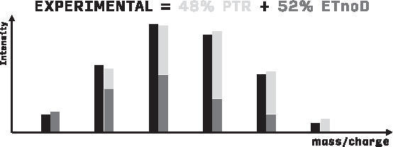
Mass spectrometry is an analytical technique of measuring the ratio of mass to charge (m/z) of molecular compounds. Ionized molecules are separated in an electromagnetic field. The intensity of the detected signal is plotted against the corresponding m/z values on a mass spectrum. In most of its range, the signal intensity is proportional to the number of detected particles (Housecroft and Constable, 2010).
Among many of its applications, mass spectrometry (MS) can be used for identifying compounds in biological samples. In the case of proteins, however, the mass of the whole molecule provides little information about its amino acidic sequence, and even less so on its tertiary structure. In particular, any permutation of amino acids in the sequence results in the same signal in the spectrum. One can gain much more insight into the structure of sample molecules by inducing their fragmentation and recording the resulting signal. In particular, knowing the masses of all consecutive fragments can reveal the protein's sequence.
There are two main approaches to protein fragmentation: bottom-up and top-down. In bottom-up proteomics, the protein is partially digested by a proteolytic enzyme and mass spectrometry is used to measure the m/z ratios of the fragments. In the top-down approach, sample proteins are subject to fragmentation only inside the mass spectrometer, without the use of any proteases.
One of the fragmentation methods used in top-down mass spectrometry is electron transfer dissociation (ETD). This ion–ion technique exploits the naturally occurring interaction between the multicharged, nonradical protein/peptide cation on one side and the radical reagent anion on the other (Syka et al., 2004; Zhurov et al., 2013). However, while this method is becoming ever more ubiquitous in the MS-based proteomic analyses, important questions remain regarding the precise reaction mechanism, fragmentation patterns, and the level(s) of protein structure that can be probed using ETD (Sohn et al., 2009, 2015). Shedding more light on the nature of ETD can thus lead to optimization of instrumental settings and overall improvement of the identification of peptide sequences and the post-translational modifications.
There are several other fragmentation techniques used in the top-down approach, most importantly collision-induced dissociation (CID), where cleavage is induced by colliding ions with nonreactive gas molecules (Wells and McLuckey, 2005). A major disadvantage of CID compared with ETD is that it often leads to loss of post-translational modifications, particularly phosphorylation (Kim and Pandey, 2012). ETD has also been found to provide more uniform fragmentation than CID, which preferentially cleaves the weakest bonds (Kim and Pandey, 2012; Zhurov et al., 2013). However, a notable amount of work has been devoted to analyzing and mathematically modeling the CID process (Wysocki et al., 2000; Zhang, 2004, 2005), while ETD has received less attention.
The fragmentation in ETD is induced by the transfer of an electron from a radical anion to the sample peptide/protein cation that after a series of electron rearrangements, results in cleavage of one of the peptide \documentclass{aastex}\usepackage{amsbsy}\usepackage{amsfonts}\usepackage{amssymb}\usepackage{bm}\usepackage{mathrsfs}\usepackage{pifont}\usepackage{stmaryrd}\usepackage{textcomp}\usepackage{portland, xspace}\usepackage{amsmath, amsxtra}\usepackage{upgreek}\pagestyle{empty}\DeclareMathSizes{10}{9}{7}{6}\begin{document}
$$( N - {C_ \alpha} )$$
\end{document} bonds. The sample cations are positively charged during the electrospray ionization (ESI) step (Fenn et al., 1989), leading to the formation of \documentclass{aastex}\usepackage{amsbsy}\usepackage{amsfonts}\usepackage{amssymb}\usepackage{bm}\usepackage{mathrsfs}\usepackage{pifont}\usepackage{stmaryrd}\usepackage{textcomp}\usepackage{portland, xspace}\usepackage{amsmath, amsxtra}\usepackage{upgreek}\pagestyle{empty}\DeclareMathSizes{10}{9}{7}{6}\begin{document}
$${ [ { \rm{M}} + { \rm{nH}} ] ^{{ \rm{n}} + }}$$
\end{document} ions, that is, adding both charge and mass to the analyte molecule M.
Apart from ETD, other reactions occur concurrently, adding their products to the signal observed in the mass spectrometer. Figure 1 presents the considered set of reactions. Unlike in ETD, during proton transfer reaction (PTR), the proton gets transferred from the protein's backbone to the anion. The mechanism of ETnoD closely resembles that of ETD, with the difference being that the protein fails to fragment into the c and z. The appearance of ETnoD fragments in the experimental data can be traced to the folding of proteins: although backbone cleavage occurs, noncovalent interactions keep the resulting fragments from separating. ETnoD can also be caused by accommodation of an electron, for example, in an aromatic side chain (Lermyte et al., 2014; Lermyte and Sobott, 2015). It is assumed that regardless of the precise reaction mechanism, the electron obtained by ETnoD causes neutralization of one ESI-generated proton (Lermyte et al., 2015a), referred to as the quenched proton further on. In all of the reactions described above, one charge is neutralized.
Considered chemical reactions. M stands for a precursor or a fragment ion, C and Z stand for fragment ions.
A single cation can undergo several reaction events, being approached multiple times by different anions. However, the so-called internal fragments of proteins, that is, resulting from two backbone cleavage events, are usually not observed, suggesting that double ETD scarcely ever occurs. On the other hand, there is a lot of evidence that one analyte molecule can undergo multiple ETnoD and PTR reactions (Lermyte et al., 2015c). Note that only molecules with nonzero charge are observed in the mass spectrometer: after a sufficiently large number of reactions, molecules simply disappear.
The isotope distributions of reaction products show considerable overlap, especially for large molecules, as illustrated in Figure 2. In particular, the products of PTR and ETnoD reactions on the same substrate differ only by 1 Da mass (the mass of the electron can be neglected, falling beyond the resolving power of most modern instruments).
Deconvolution of the observed isotopic envelopes performed by MassTodon. The observed signal is represented as a combination of a number of theoretical isotopic patterns.
The peptide bond cleavage induced by ETD is believed to be fairly uniform (Li et al., 2011). A notable exception from this rule is the peptide bond of proline: due to the ring structure of this amino acid, the c and z ions are held together even after the \documentclass{aastex}\usepackage{amsbsy}\usepackage{amsfonts}\usepackage{amssymb}\usepackage{bm}\usepackage{mathrsfs}\usepackage{pifont}\usepackage{stmaryrd}\usepackage{textcomp}\usepackage{portland, xspace}\usepackage{amsmath, amsxtra}\usepackage{upgreek}\pagestyle{empty}\DeclareMathSizes{10}{9}{7}{6}\begin{document}
$$N - {C_ \alpha }$$
\end{document} bond cleavage.
A specific type of \documentclass{aastex}\usepackage{amsbsy}\usepackage{amsfonts}\usepackage{amssymb}\usepackage{bm}\usepackage{mathrsfs}\usepackage{pifont}\usepackage{stmaryrd}\usepackage{textcomp}\usepackage{portland, xspace}\usepackage{amsmath, amsxtra}\usepackage{upgreek}\pagestyle{empty}\DeclareMathSizes{10}{9}{7}{6}\begin{document}
$$N - {C_ \alpha }$$
\end{document} bond cleavage occurs on the N-terminus, leading to a loss of one ammonia molecule. The precise mechanism of this reaction is not yet known. In this study, we assume this reaction to be an instance of ETD and treat the ammonia molecule as a c fragment. Therefore, the number of considered ETD cleavage sites is equal to the number of amino acids other than proline in the protein/peptide sequence.
1.1. Our contribution
We propose a formal model of the electron-driven reactions occurring inside the mass spectrometer. We follow a modeling strategy first developed by Gambin and Kluge (2010) to study the degradation of proteins by proteolytic enzymes. The model of ETD reaction can be obtained conceptually in the same way: the stochastic description of the reaction, based on a Markov jump process (MJP), is transformed to a populational description of a large number of molecules based on a system of ordinary differential equations (ODEs). Given the intensities of transitions in the process, we solve the ODEs numerically with a recursive algorithm to obtain the expected number of molecules. The space of possible intensities is then searched for the best possible set of parameters by solving an optimization problem.
The model we propose lets us express the mass spectrum in terms of parameters such as the total intensity of reactions and the probabilities of the three studied reactions: ETD, PTR, and ETnoD. A process described by a handful of parameters can be easily visualized and thus easily understood. In addition, the comparison of different spectra, for example, coming from different instrument settings, is highly simplified.
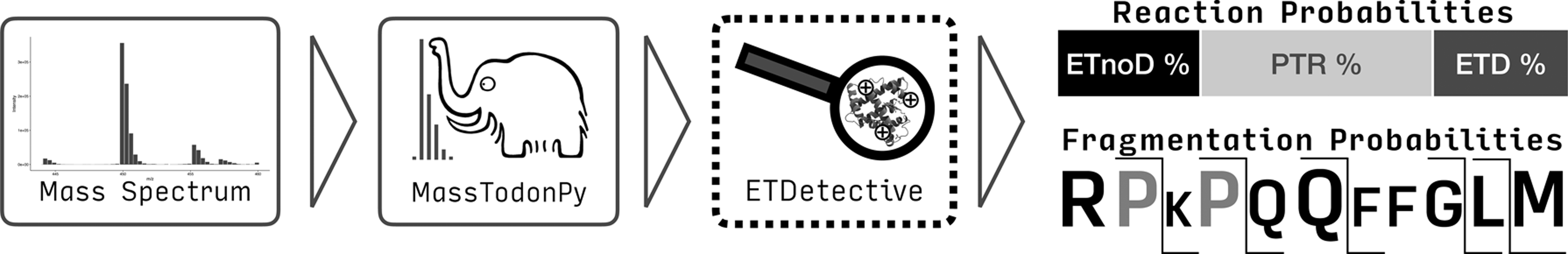
We apply our method to mass spectra gathered in controlled experiments obtained for highly purified compounds. The identity of the precursor ion and all fragments obtained given a set of possible reactions is known and the quantities of these fragments can be established using our in-house developed identification tool called MassTodon (Lermyte et al., 2015a, 2017; Łącki, et al., 2017). Given a mass spectrum and a precursor molecule, MassTodon outputs a list of reaction products together with their estimated intensities (that are usually assumed to be proportional to the actual number of ions). It performs deisotropization and deconvolution of the spectrum, that is, it reports total intensities of chemical compounds in possibly overlapping isotope clusters (Fig. 2).
The model and the fitting procedure have been implemented in Python. The software tool, called ETDetective, is designed as an extension to MassTodon workflow, see https://matteolacki.github.io/MassTodonPy. The control flow of the whole process from obtaining a spectrum to obtaining the reaction rates and fragmentation patterns has been depicted in Figure 3. ETDetective together with example data is available for download at https://github.com/mciach/ETDetective under the two-clause BSD license.
The process of mass spectrum interpretation with MassTodon and ETDetective. ETD, electron transfer dissociation.
1.2. Related research
Various approaches have been taken to model different protein fragmentation techniques (Breuker et al., 2004; Simons, 2010; Tureček and Julian, 2013; Zhurov et al., 2013). A somewhat similar approach to the one taken by us was presented by Zhang (2004, 2005) to study CID fragmentation, who uses a kinetic model to study fragmentation. Zhang (2010) adapts the model to model mass spectra obtained with the use of ETD. The model uses 280 parameters and its derivation is grounded in the theory of statistical mechanics. The model was fitted to a training data set consisting of more than 7000 ETD spectra simultaneously.
There are important differences between that approach and ours. Zhang's model is derived from the first principles of statistical physics, whereas the one we propose is more phenomenological. In our approach, the physics of the phenomenon dictates only the potential states and the transitions between them. We then cast the problem into the well-studied setting of continuous time MJPs. Our current approach also builds upon the approach for parameter estimation introduced previously in the MassTodon article. MassTodon used a heuristical approach to estimate some of the deep parameters of the process, relying on the idea of parsimony.
The approach we present here is theory driven. That said, ETDetective can use some of the estimates provided by MassTodon and not optimize them. This can greatly reduce the number of existing parameters as one can skip the estimation of fragmentation probabilities. In contrast, parameters described by Zhang are fairly complex, making it more difficult to limit their number. Limiting the number of parameters also reduces the risk of model's unidentifiability. Finally, one can use the results obtained using our model as an input for another model that (similarly to Zhang) includes more of the underlying physical principles. For instance, the reaction rates we provide appear in the Arrhenius equations.
Apart from these mostly theoretical considerations, the ability to fit to individual mass spectra also simplifies the process of comparing results obtained with different instruments. This is an important step in experiment design (see Lermyte et al., 2015a).
A notable amount of literature has been built up around the idea of purely data-driven prediction of the intensity of peptides in tandem MS experiments (Elias et al., 2004; Arnold et al., 2006; Degroeve et al., 2013). A more exploratory approach targeted at studying fragmentation patterns was taken by Li et al. (2011). However, the above approaches have been applied mainly to study CID.
1.3. Organization of the article
First, we introduce the theoretical considerations behind our model. Then, we describe the procedures used to obtain our data sets (experimental and in silico). Then, we assess the performance of the model. Finally, we discuss existing problems and possible extensions.
2. Formal Model of the ETD Reaction
2.1. Statement of the model
Following the ideas outlined in Gambin and Kluge (2010), we model ETD and its side reactions as a continuous time MJP, which is a well-established approach to modeling chemical reactions. Below, we describe the state space of our model and provide elementary lemmas on its size and properties. Next, we define the transition intensities of our MJP.
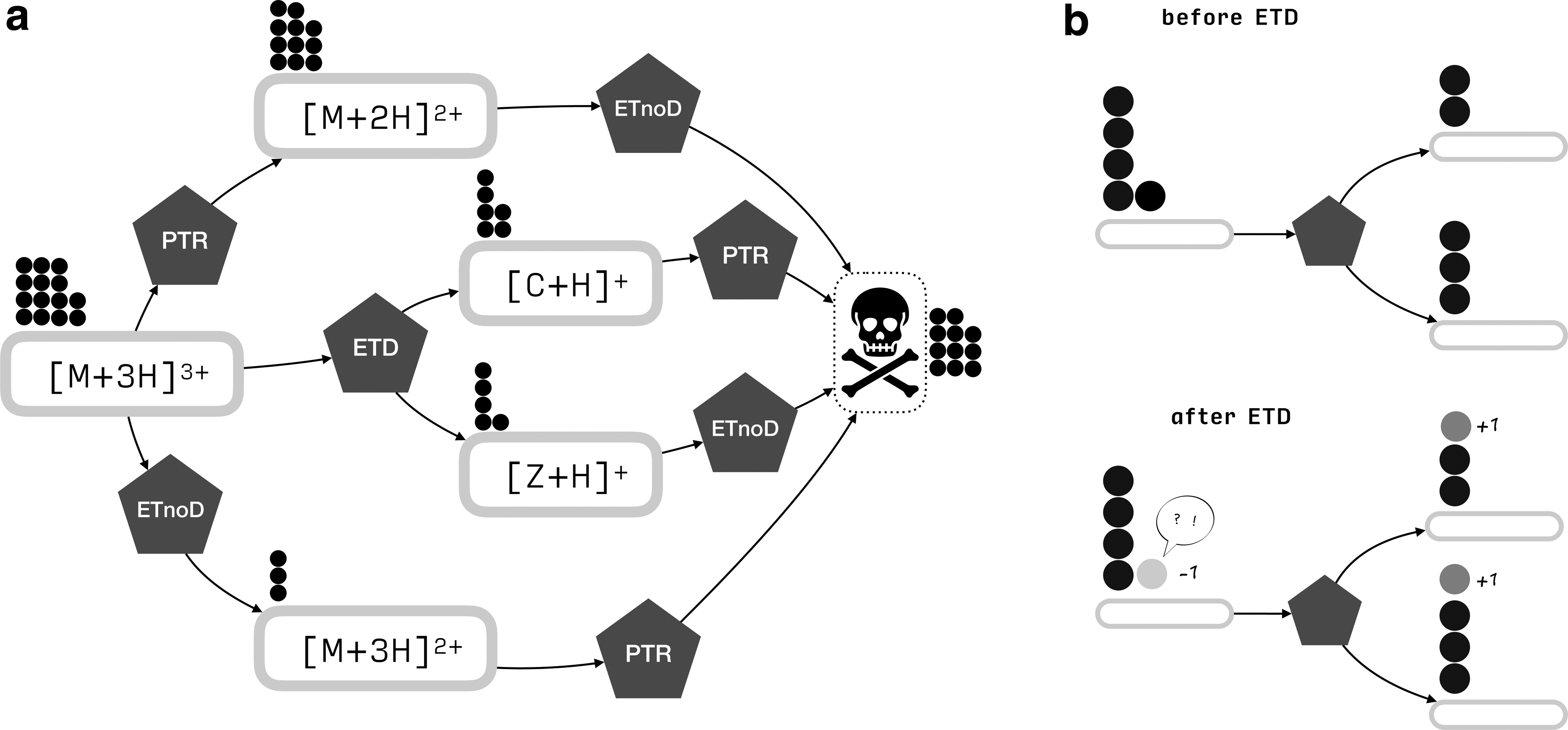
Our model can be described by a Petri net, in which places correspond to molecular species, transitions to reactions, and tokens to molecules of a given species (Fig. 4).
A model of the ETD reaction. (a) A fragment of the reaction graph for a triply charged precursor. The molecular species are depicted as ovals and the reactions as pentagons. The skull represents the cemetery. The reaction graph serves as a board for tokens that represent the numbers of molecules of a given species, depicted as circles. Only one ETD transition has been shown for clarity of the image. (b) During each reaction, a token disappears on the substrate side and product tokens appear: one in the case of ETnoD and PTR, two in the case of ETD.
All molecules that cannot be observed, for example, the internal fragments or ions in which all charges have been neutralized, are merged into the cemetery—a unique place without any outgoing transitions. Note, however, the reactions that yield such molecules are still present in the graph. We will refer to this net as the reaction graph.
Definition 1. A reaction graph is a bipartite, directed connected graph\documentclass{aastex}\usepackage{amsbsy}\usepackage{amsfonts}\usepackage{amssymb}\usepackage{bm}\usepackage{mathrsfs}\usepackage{pifont}\usepackage{stmaryrd}\usepackage{textcomp}\usepackage{portland, xspace}\usepackage{amsmath, amsxtra}\usepackage{upgreek}\pagestyle{empty}\DeclareMathSizes{10}{9}{7}{6}\begin{document}
$$\langle \mathcal{M} , \mathcal{R} , \mathcal{F} \rangle$$
\end{document}, in which
• \documentclass{aastex}\usepackage{amsbsy}\usepackage{amsfonts}\usepackage{amssymb}\usepackage{bm}\usepackage{mathrsfs}\usepackage{pifont}\usepackage{stmaryrd}\usepackage{textcomp}\usepackage{portland, xspace}\usepackage{amsmath, amsxtra}\usepackage{upgreek}\pagestyle{empty}\DeclareMathSizes{10}{9}{7}{6}\begin{document}
$$\mathcal{M}$$
\end{document}is a set of vertices called molecular species or places.
• \documentclass{aastex}\usepackage{amsbsy}\usepackage{amsfonts}\usepackage{amssymb}\usepackage{bm}\usepackage{mathrsfs}\usepackage{pifont}\usepackage{stmaryrd}\usepackage{textcomp}\usepackage{portland, xspace}\usepackage{amsmath, amsxtra}\usepackage{upgreek}\pagestyle{empty}\DeclareMathSizes{10}{9}{7}{6}\begin{document}
$$\mathcal{R}$$
\end{document}is a set of vertices called reactions or transitions.
• \documentclass{aastex}\usepackage{amsbsy}\usepackage{amsfonts}\usepackage{amssymb}\usepackage{bm}\usepackage{mathrsfs}\usepackage{pifont}\usepackage{stmaryrd}\usepackage{textcomp}\usepackage{portland, xspace}\usepackage{amsmath, amsxtra}\usepackage{upgreek}\pagestyle{empty}\DeclareMathSizes{10}{9}{7}{6}\begin{document}
$$\mathcal{F} \subset ( \mathcal{M} \times \mathcal{R} ) \cup ( \mathcal{R} \times \mathcal{M} )$$
\end{document}is a set of edges connecting species and reactions.
• \documentclass{aastex}\usepackage{amsbsy}\usepackage{amsfonts}\usepackage{amssymb}\usepackage{bm}\usepackage{mathrsfs}\usepackage{pifont}\usepackage{stmaryrd}\usepackage{textcomp}\usepackage{portland, xspace}\usepackage{amsmath, amsxtra}\usepackage{upgreek}\pagestyle{empty}\DeclareMathSizes{10}{9}{7}{6}\begin{document}
$$W: \mathcal{M} \to \mathbb{N}$$
\end{document}is a function denoting the number of molecules or tokens of a molecular species.
Each molecular species \documentclass{aastex}\usepackage{amsbsy}\usepackage{amsfonts}\usepackage{amssymb}\usepackage{bm}\usepackage{mathrsfs}\usepackage{pifont}\usepackage{stmaryrd}\usepackage{textcomp}\usepackage{portland, xspace}\usepackage{amsmath, amsxtra}\usepackage{upgreek}\pagestyle{empty}\DeclareMathSizes{10}{9}{7}{6}\begin{document}
$$u \in \mathcal{M}$$
\end{document} is described by the sequence of amino acids s, the charge of the cation q, and the number of quenched protons g so that \documentclass{aastex}\usepackage{amsbsy}\usepackage{amsfonts}\usepackage{amssymb}\usepackage{bm}\usepackage{mathrsfs}\usepackage{pifont}\usepackage{stmaryrd}\usepackage{textcomp}\usepackage{portland, xspace}\usepackage{amsmath, amsxtra}\usepackage{upgreek}\pagestyle{empty}\DeclareMathSizes{10}{9}{7}{6}\begin{document}
$$u = ( s , q , g )$$
\end{document}. Note that we do not model the positions of the charges, that is, we assume to know only the numbers of protons on the backbone. We denote the charge of u as qu. The sequence and number of quenched protons are denoted accordingly as su and gu.
The precursor or root of the reaction graph, denoted as \documentclass{aastex}\usepackage{amsbsy}\usepackage{amsfonts}\usepackage{amssymb}\usepackage{bm}\usepackage{mathrsfs}\usepackage{pifont}\usepackage{stmaryrd}\usepackage{textcomp}\usepackage{portland, xspace}\usepackage{amsmath, amsxtra}\usepackage{upgreek}\pagestyle{empty}\DeclareMathSizes{10}{9}{7}{6}\begin{document}
$$r = ( s , {q_0} , 0 )$$
\end{document}, is the unique molecular species with no incoming transitions (i.e., the root of the reaction graph). Based on the description of the set of molecular species, we can approximate the size of this set as follows:
Lemma 1.The number of the places in a reaction graph corresponding to a precursor molecule\documentclass{aastex}\usepackage{amsbsy}\usepackage{amsfonts}\usepackage{amssymb}\usepackage{bm}\usepackage{mathrsfs}\usepackage{pifont}\usepackage{stmaryrd}\usepackage{textcomp}\usepackage{portland, xspace}\usepackage{amsmath, amsxtra}\usepackage{upgreek}\pagestyle{empty}\DeclareMathSizes{10}{9}{7}{6}\begin{document}
$$r = ( s , {q_0} , 0 )$$
\end{document}is\documentclass{aastex}\usepackage{amsbsy}\usepackage{amsfonts}\usepackage{amssymb}\usepackage{bm}\usepackage{mathrsfs}\usepackage{pifont}\usepackage{stmaryrd}\usepackage{textcomp}\usepackage{portland, xspace}\usepackage{amsmath, amsxtra}\usepackage{upgreek}\pagestyle{empty}\DeclareMathSizes{10}{9}{7}{6}\begin{document}
$$O ( Lq_0^2 )$$
\end{document}, where L is the length of s.
Proof. Since in the reaction graph we do not include the internal fragments (i.e., infixes of the amino acid sequence), there are \documentclass{aastex}\usepackage{amsbsy}\usepackage{amsfonts}\usepackage{amssymb}\usepackage{bm}\usepackage{mathrsfs}\usepackage{pifont}\usepackage{stmaryrd}\usepackage{textcomp}\usepackage{portland, xspace}\usepackage{amsmath, amsxtra}\usepackage{upgreek}\pagestyle{empty}\DeclareMathSizes{10}{9}{7}{6}\begin{document}
$$O ( L )$$
\end{document} possible sequences of molecular species. Furthermore, for each molecular species \documentclass{aastex}\usepackage{amsbsy}\usepackage{amsfonts}\usepackage{amssymb}\usepackage{bm}\usepackage{mathrsfs}\usepackage{pifont}\usepackage{stmaryrd}\usepackage{textcomp}\usepackage{portland, xspace}\usepackage{amsmath, amsxtra}\usepackage{upgreek}\pagestyle{empty}\DeclareMathSizes{10}{9}{7}{6}\begin{document}
$$u = ( {s_u} , {q_u} , {g_u} )$$
\end{document}, we have \documentclass{aastex}\usepackage{amsbsy}\usepackage{amsfonts}\usepackage{amssymb}\usepackage{bm}\usepackage{mathrsfs}\usepackage{pifont}\usepackage{stmaryrd}\usepackage{textcomp}\usepackage{portland, xspace}\usepackage{amsmath, amsxtra}\usepackage{upgreek}\pagestyle{empty}\DeclareMathSizes{10}{9}{7}{6}\begin{document}
$${q_u} + {g_u} \le q$$
\end{document}. ■
For two molecular species u and v, we write \documentclass{aastex}\usepackage{amsbsy}\usepackage{amsfonts}\usepackage{amssymb}\usepackage{bm}\usepackage{mathrsfs}\usepackage{pifont}\usepackage{stmaryrd}\usepackage{textcomp}\usepackage{portland, xspace}\usepackage{amsmath, amsxtra}\usepackage{upgreek}\pagestyle{empty}\DeclareMathSizes{10}{9}{7}{6}\begin{document}
$$u \to v$$
\end{document} if v can be reached from u by a single reaction. We write \documentclass{aastex}\usepackage{amsbsy}\usepackage{amsfonts}\usepackage{amssymb}\usepackage{bm}\usepackage{mathrsfs}\usepackage{pifont}\usepackage{stmaryrd}\usepackage{textcomp}\usepackage{portland, xspace}\usepackage{amsmath, amsxtra}\usepackage{upgreek}\pagestyle{empty}\DeclareMathSizes{10}{9}{7}{6}\begin{document}
$$u \ge v$$
\end{document} if there exist molecular species \documentclass{aastex}\usepackage{amsbsy}\usepackage{amsfonts}\usepackage{amssymb}\usepackage{bm}\usepackage{mathrsfs}\usepackage{pifont}\usepackage{stmaryrd}\usepackage{textcomp}\usepackage{portland, xspace}\usepackage{amsmath, amsxtra}\usepackage{upgreek}\pagestyle{empty}\DeclareMathSizes{10}{9}{7}{6}\begin{document}
$${m_1} , {m_2} , \ldots , {m_n}$$
\end{document} such that \documentclass{aastex}\usepackage{amsbsy}\usepackage{amsfonts}\usepackage{amssymb}\usepackage{bm}\usepackage{mathrsfs}\usepackage{pifont}\usepackage{stmaryrd}\usepackage{textcomp}\usepackage{portland, xspace}\usepackage{amsmath, amsxtra}\usepackage{upgreek}\pagestyle{empty}\DeclareMathSizes{10}{9}{7}{6}\begin{document}
$$u = {m_1} \to {m_2} \to \cdots \to {m_n} = v$$
\end{document}. Note that \documentclass{aastex}\usepackage{amsbsy}\usepackage{amsfonts}\usepackage{amssymb}\usepackage{bm}\usepackage{mathrsfs}\usepackage{pifont}\usepackage{stmaryrd}\usepackage{textcomp}\usepackage{portland, xspace}\usepackage{amsmath, amsxtra}\usepackage{upgreek}\pagestyle{empty}\DeclareMathSizes{10}{9}{7}{6}\begin{document}
$$u \ge u$$
\end{document}. We also write \documentclass{aastex}\usepackage{amsbsy}\usepackage{amsfonts}\usepackage{amssymb}\usepackage{bm}\usepackage{mathrsfs}\usepackage{pifont}\usepackage{stmaryrd}\usepackage{textcomp}\usepackage{portland, xspace}\usepackage{amsmath, amsxtra}\usepackage{upgreek}\pagestyle{empty}\DeclareMathSizes{10}{9}{7}{6}\begin{document}
$$u > v$$
\end{document} if \documentclass{aastex}\usepackage{amsbsy}\usepackage{amsfonts}\usepackage{amssymb}\usepackage{bm}\usepackage{mathrsfs}\usepackage{pifont}\usepackage{stmaryrd}\usepackage{textcomp}\usepackage{portland, xspace}\usepackage{amsmath, amsxtra}\usepackage{upgreek}\pagestyle{empty}\DeclareMathSizes{10}{9}{7}{6}\begin{document}
$$u \ge v$$
\end{document} and \documentclass{aastex}\usepackage{amsbsy}\usepackage{amsfonts}\usepackage{amssymb}\usepackage{bm}\usepackage{mathrsfs}\usepackage{pifont}\usepackage{stmaryrd}\usepackage{textcomp}\usepackage{portland, xspace}\usepackage{amsmath, amsxtra}\usepackage{upgreek}\pagestyle{empty}\DeclareMathSizes{10}{9}{7}{6}\begin{document}
$$u \ne v$$
\end{document}. In this case, u is referred to as the ancestor or ancestral molecule of v.
For a reaction \documentclass{aastex}\usepackage{amsbsy}\usepackage{amsfonts}\usepackage{amssymb}\usepackage{bm}\usepackage{mathrsfs}\usepackage{pifont}\usepackage{stmaryrd}\usepackage{textcomp}\usepackage{portland, xspace}\usepackage{amsmath, amsxtra}\usepackage{upgreek}\pagestyle{empty}\DeclareMathSizes{10}{9}{7}{6}\begin{document}
$$R \in \mathcal{R}$$
\end{document}, all molecules u such that \documentclass{aastex}\usepackage{amsbsy}\usepackage{amsfonts}\usepackage{amssymb}\usepackage{bm}\usepackage{mathrsfs}\usepackage{pifont}\usepackage{stmaryrd}\usepackage{textcomp}\usepackage{portland, xspace}\usepackage{amsmath, amsxtra}\usepackage{upgreek}\pagestyle{empty}\DeclareMathSizes{10}{9}{7}{6}\begin{document}
$$( u , R ) \in \mathcal{F}$$
\end{document} are called substrates of R. Similarly, all molecules v such that \documentclass{aastex}\usepackage{amsbsy}\usepackage{amsfonts}\usepackage{amssymb}\usepackage{bm}\usepackage{mathrsfs}\usepackage{pifont}\usepackage{stmaryrd}\usepackage{textcomp}\usepackage{portland, xspace}\usepackage{amsmath, amsxtra}\usepackage{upgreek}\pagestyle{empty}\DeclareMathSizes{10}{9}{7}{6}\begin{document}
$$( R , v ) \in \mathcal{F}$$
\end{document} are called products of R. If u is the substrate of reaction \documentclass{aastex}\usepackage{amsbsy}\usepackage{amsfonts}\usepackage{amssymb}\usepackage{bm}\usepackage{mathrsfs}\usepackage{pifont}\usepackage{stmaryrd}\usepackage{textcomp}\usepackage{portland, xspace}\usepackage{amsmath, amsxtra}\usepackage{upgreek}\pagestyle{empty}\DeclareMathSizes{10}{9}{7}{6}\begin{document}
$$R \in \mathcal{R}$$
\end{document} and \documentclass{aastex}\usepackage{amsbsy}\usepackage{amsfonts}\usepackage{amssymb}\usepackage{bm}\usepackage{mathrsfs}\usepackage{pifont}\usepackage{stmaryrd}\usepackage{textcomp}\usepackage{portland, xspace}\usepackage{amsmath, amsxtra}\usepackage{upgreek}\pagestyle{empty}\DeclareMathSizes{10}{9}{7}{6}\begin{document}
$${v_1} , {v_2} , \ldots , {v_m}$$
\end{document} are its products, then we denote R as \documentclass{aastex}\usepackage{amsbsy}\usepackage{amsfonts}\usepackage{amssymb}\usepackage{bm}\usepackage{mathrsfs}\usepackage{pifont}\usepackage{stmaryrd}\usepackage{textcomp}\usepackage{portland, xspace}\usepackage{amsmath, amsxtra}\usepackage{upgreek}\pagestyle{empty}\DeclareMathSizes{10}{9}{7}{6}\begin{document}
$$u \to {v_1} + {v_2} + \cdots + {v_m}$$
\end{document}. Species vi are referred to as the daughter species of ui, and ui are called parent species of vi.
Note that in our model, any reaction can be uniquely identified by its substrate and one of the products. Therefore, we will write \documentclass{aastex}\usepackage{amsbsy}\usepackage{amsfonts}\usepackage{amssymb}\usepackage{bm}\usepackage{mathrsfs}\usepackage{pifont}\usepackage{stmaryrd}\usepackage{textcomp}\usepackage{portland, xspace}\usepackage{amsmath, amsxtra}\usepackage{upgreek}\pagestyle{empty}\DeclareMathSizes{10}{9}{7}{6}\begin{document}
$$u \to {v_1}$$
\end{document} or \documentclass{aastex}\usepackage{amsbsy}\usepackage{amsfonts}\usepackage{amssymb}\usepackage{bm}\usepackage{mathrsfs}\usepackage{pifont}\usepackage{stmaryrd}\usepackage{textcomp}\usepackage{portland, xspace}\usepackage{amsmath, amsxtra}\usepackage{upgreek}\pagestyle{empty}\DeclareMathSizes{10}{9}{7}{6}\begin{document}
$$u \to {v_2}$$
\end{document} to denote a reaction \documentclass{aastex}\usepackage{amsbsy}\usepackage{amsfonts}\usepackage{amssymb}\usepackage{bm}\usepackage{mathrsfs}\usepackage{pifont}\usepackage{stmaryrd}\usepackage{textcomp}\usepackage{portland, xspace}\usepackage{amsmath, amsxtra}\usepackage{upgreek}\pagestyle{empty}\DeclareMathSizes{10}{9}{7}{6}\begin{document}
$$u \to {v_1} + {v_2}$$
\end{document}. We will also write \documentclass{aastex}\usepackage{amsbsy}\usepackage{amsfonts}\usepackage{amssymb}\usepackage{bm}\usepackage{mathrsfs}\usepackage{pifont}\usepackage{stmaryrd}\usepackage{textcomp}\usepackage{portland, xspace}\usepackage{amsmath, amsxtra}\usepackage{upgreek}\pagestyle{empty}\DeclareMathSizes{10}{9}{7}{6}\begin{document}
$$u \to v$$
\end{document} to indicate the existence of a reaction for which u is a substrate and v is a product.
We assume that at the onset, before any reaction occurred, positive charges are attached randomly to basic amino acids of the molecules, that is, on lysines, arginines, and histidines, at most one charge per site. This restricts the number of protons on a molecular species: for any molecule, m, \documentclass{aastex}\usepackage{amsbsy}\usepackage{amsfonts}\usepackage{amssymb}\usepackage{bm}\usepackage{mathrsfs}\usepackage{pifont}\usepackage{stmaryrd}\usepackage{textcomp}\usepackage{portland, xspace}\usepackage{amsmath, amsxtra}\usepackage{upgreek}\pagestyle{empty}\DeclareMathSizes{10}{9}{7}{6}\begin{document}
$${q_m} + {g_m} \le {B_m}$$
\end{document} must hold, where Bm is the number of basic amino acids in its sequence.
If one does not know the position of charges before ETD, then one cannot know how many protons should appear on the fragment ions. Therefore, a single fragmentation reaction at a given residue gives rise to several different outcomes. This leads to the following lemma. We have the following lemma:
Lemma 2.Assume a random placement of charges and quenched protons on basic amino acids of a molecule\documentclass{aastex}\usepackage{amsbsy}\usepackage{amsfonts}\usepackage{amssymb}\usepackage{bm}\usepackage{mathrsfs}\usepackage{pifont}\usepackage{stmaryrd}\usepackage{textcomp}\usepackage{portland, xspace}\usepackage{amsmath, amsxtra}\usepackage{upgreek}\pagestyle{empty}\DeclareMathSizes{10}{9}{7}{6}\begin{document}
$$m = ( s , q , g )$$
\end{document}. Let cl be the l-th prefix of the sequence, and let\documentclass{aastex}\usepackage{amsbsy}\usepackage{amsfonts}\usepackage{amssymb}\usepackage{bm}\usepackage{mathrsfs}\usepackage{pifont}\usepackage{stmaryrd}\usepackage{textcomp}\usepackage{portland, xspace}\usepackage{amsmath, amsxtra}\usepackage{upgreek}\pagestyle{empty}\DeclareMathSizes{10}{9}{7}{6}\begin{document}
$${z_{L - l}}$$
\end{document}be the l-th suffix. Let Bc be the number of basic amino acids in the backbone of cl, and Bz be the number of basic amino acids on the backbone of the corresponding\documentclass{aastex}\usepackage{amsbsy}\usepackage{amsfonts}\usepackage{amssymb}\usepackage{bm}\usepackage{mathrsfs}\usepackage{pifont}\usepackage{stmaryrd}\usepackage{textcomp}\usepackage{portland, xspace}\usepackage{amsmath, amsxtra}\usepackage{upgreek}\pagestyle{empty}\DeclareMathSizes{10}{9}{7}{6}\begin{document}
$${z_{L - l}}$$
\end{document}fragment. Then, the probability of observing qc charges and gc quenched protons on cl after ETD cleavage on l-th amino acid is equal to\documentclass{aastex}\usepackage{amsbsy}\usepackage{amsfonts}\usepackage{amssymb}\usepackage{bm}\usepackage{mathrsfs}\usepackage{pifont}\usepackage{stmaryrd}\usepackage{textcomp}\usepackage{portland, xspace}\usepackage{amsmath, amsxtra}\usepackage{upgreek}\pagestyle{empty}\DeclareMathSizes{10}{9}{7}{6}\begin{document}
\begin{align*}
{ P_l } ( { q_c } , { g_c } ) = { \frac { \left( { \begin{matrix} { { B_c } } \\ { { q_c } } \\ \end{matrix}} \right)
\left( { \begin{matrix} { { B_z } } \\ { q - 1 - { q_c } } \\
\end{matrix}} \right) } { \left( { \begin{matrix} { { B_c
} + { B_z } } \\ { q - 1 } \\ \end{matrix} } \right) } } { \frac {
\left( { \begin{matrix} { { B_c } - { q_c } } \\ { { g_c } }
\\ \end{matrix}} \right) \left( { \begin{matrix} { { B_z }
- q + { q_c } + 1 } \\ { g - { g_c } } \\ \end{matrix}} \right) }
{ \left( { \begin{matrix} { { B_c } + { B_z } - q + 1 } \\ g
\\ \end{matrix}} \right) } } ,
\end{align*}
\end{document}
and also equal to the probability of observing\documentclass{aastex}\usepackage{amsbsy}\usepackage{amsfonts}\usepackage{amssymb}\usepackage{bm}\usepackage{mathrsfs}\usepackage{pifont}\usepackage{stmaryrd}\usepackage{textcomp}\usepackage{portland, xspace}\usepackage{amsmath, amsxtra}\usepackage{upgreek}\pagestyle{empty}\DeclareMathSizes{10}{9}{7}{6}\begin{document}
$${q_z} = q - 1 - {q_c}$$
\end{document}charges and\documentclass{aastex}\usepackage{amsbsy}\usepackage{amsfonts}\usepackage{amssymb}\usepackage{bm}\usepackage{mathrsfs}\usepackage{pifont}\usepackage{stmaryrd}\usepackage{textcomp}\usepackage{portland, xspace}\usepackage{amsmath, amsxtra}\usepackage{upgreek}\pagestyle{empty}\DeclareMathSizes{10}{9}{7}{6}\begin{document}
$${g_z} = g - {g_c}$$
\end{document}quenched protons on\documentclass{aastex}\usepackage{amsbsy}\usepackage{amsfonts}\usepackage{amssymb}\usepackage{bm}\usepackage{mathrsfs}\usepackage{pifont}\usepackage{stmaryrd}\usepackage{textcomp}\usepackage{portland, xspace}\usepackage{amsmath, amsxtra}\usepackage{upgreek}\pagestyle{empty}\DeclareMathSizes{10}{9}{7}{6}\begin{document}
$${z_{L - l}}$$
\end{document}.
Proof. Since one charge gets neutralized during the reaction, both fragments have \documentclass{aastex}\usepackage{amsbsy}\usepackage{amsfonts}\usepackage{amssymb}\usepackage{bm}\usepackage{mathrsfs}\usepackage{pifont}\usepackage{stmaryrd}\usepackage{textcomp}\usepackage{portland, xspace}\usepackage{amsmath, amsxtra}\usepackage{upgreek}\pagestyle{empty}\DeclareMathSizes{10}{9}{7}{6}\begin{document}
$$q - 1$$
\end{document} charges and g quenched protons in total. As each charge is placed randomly and independently of other charges on the unoccupied basic sites, the probability of observing qc charges on cl is equal to the probability of choosing qc of Bc basic amino acids and \documentclass{aastex}\usepackage{amsbsy}\usepackage{amsfonts}\usepackage{amssymb}\usepackage{bm}\usepackage{mathrsfs}\usepackage{pifont}\usepackage{stmaryrd}\usepackage{textcomp}\usepackage{portland, xspace}\usepackage{amsmath, amsxtra}\usepackage{upgreek}\pagestyle{empty}\DeclareMathSizes{10}{9}{7}{6}\begin{document}
$$q - 1 - {q_c}$$
\end{document} of Bz basic amino acids randomly and without replacement. After placing the charges on the sequence, there are \documentclass{aastex}\usepackage{amsbsy}\usepackage{amsfonts}\usepackage{amssymb}\usepackage{bm}\usepackage{mathrsfs}\usepackage{pifont}\usepackage{stmaryrd}\usepackage{textcomp}\usepackage{portland, xspace}\usepackage{amsmath, amsxtra}\usepackage{upgreek}\pagestyle{empty}\DeclareMathSizes{10}{9}{7}{6}\begin{document}
$${B_c} + {B_z} - q + 1$$
\end{document} unoccupied basic sites. The probability of observing gc quenched protons on cl, given qc charges, is then equal to the probability of choosing gc of \documentclass{aastex}\usepackage{amsbsy}\usepackage{amsfonts}\usepackage{amssymb}\usepackage{bm}\usepackage{mathrsfs}\usepackage{pifont}\usepackage{stmaryrd}\usepackage{textcomp}\usepackage{portland, xspace}\usepackage{amsmath, amsxtra}\usepackage{upgreek}\pagestyle{empty}\DeclareMathSizes{10}{9}{7}{6}\begin{document}
$${B_c} - {q_c}$$
\end{document} basic amino acids and \documentclass{aastex}\usepackage{amsbsy}\usepackage{amsfonts}\usepackage{amssymb}\usepackage{bm}\usepackage{mathrsfs}\usepackage{pifont}\usepackage{stmaryrd}\usepackage{textcomp}\usepackage{portland, xspace}\usepackage{amsmath, amsxtra}\usepackage{upgreek}\pagestyle{empty}\DeclareMathSizes{10}{9}{7}{6}\begin{document}
$$g - {g_c}$$
\end{document} of \documentclass{aastex}\usepackage{amsbsy}\usepackage{amsfonts}\usepackage{amssymb}\usepackage{bm}\usepackage{mathrsfs}\usepackage{pifont}\usepackage{stmaryrd}\usepackage{textcomp}\usepackage{portland, xspace}\usepackage{amsmath, amsxtra}\usepackage{upgreek}\pagestyle{empty}\DeclareMathSizes{10}{9}{7}{6}\begin{document}
$${B_z} - ( q - 1 - {q_c} )$$
\end{document} basic amino acids. ■
The outcomes of the PTR and ETnoD reactions are unique. It follows that the number of outgoing transitions for a molecular species other than the cemetery is equal to the number of ETD transitions plus two side reactions:
\documentclass{aastex}\usepackage{amsbsy}\usepackage{amsfonts}\usepackage{amssymb}\usepackage{bm}\usepackage{mathrsfs}\usepackage{pifont}\usepackage{stmaryrd}\usepackage{textcomp}\usepackage{portland, xspace}\usepackage{amsmath, amsxtra}\usepackage{upgreek}\pagestyle{empty}\DeclareMathSizes{10}{9}{7}{6}\begin{document}
\begin{align*}
2 + \sum \limits_{l = 1}^L \left( { \begin{matrix} {{B_{{c_l}}} + {B_{{z_{L - l}}}}} \\ {q - 1} \\ \end{matrix} } \right) \left( { \begin{matrix} {{B_{{c_l}}} + {B_{{z_{L - l}}}} - q + 1} \\ g \\ \end{matrix} } \right).
\end{align*}
\end{document}
However, many transitions lead directly to the cemetery. This is especially the case for any molecule with a single charge or any ETD reaction of a molecular species that has already undergone an ETD.
The rate of a reaction \documentclass{aastex}\usepackage{amsbsy}\usepackage{amsfonts}\usepackage{amssymb}\usepackage{bm}\usepackage{mathrsfs}\usepackage{pifont}\usepackage{stmaryrd}\usepackage{textcomp}\usepackage{portland, xspace}\usepackage{amsmath, amsxtra}\usepackage{upgreek}\pagestyle{empty}\DeclareMathSizes{10}{9}{7}{6}\begin{document}
$$R = u \to v$$
\end{document} is denoted as \documentclass{aastex}\usepackage{amsbsy}\usepackage{amsfonts}\usepackage{amssymb}\usepackage{bm}\usepackage{mathrsfs}\usepackage{pifont}\usepackage{stmaryrd}\usepackage{textcomp}\usepackage{portland, xspace}\usepackage{amsmath, amsxtra}\usepackage{upgreek}\pagestyle{empty}\DeclareMathSizes{10}{9}{7}{6}\begin{document}
$${ \lambda _{uv}}$$
\end{document}. We assume that this rate can be factorized into a product of base reaction intensity I, squared charge of the substrate qu, and reaction probability PR so that
\documentclass{aastex}\usepackage{amsbsy}\usepackage{amsfonts}\usepackage{amssymb}\usepackage{bm}\usepackage{mathrsfs}\usepackage{pifont}\usepackage{stmaryrd}\usepackage{textcomp}\usepackage{portland, xspace}\usepackage{amsmath, amsxtra}\usepackage{upgreek}\pagestyle{empty}\DeclareMathSizes{10}{9}{7}{6}\begin{document}
\begin{align*}
{ \lambda _{uv}} = Iq_u^2{P_R}{ \kern 1pt} \;for \;{ \kern 1pt} R = u \to v ,
\end{align*}
\end{document}
In the above definition, \documentclass{aastex}\usepackage{amsbsy}\usepackage{amsfonts}\usepackage{amssymb}\usepackage{bm}\usepackage{mathrsfs}\usepackage{pifont}\usepackage{stmaryrd}\usepackage{textcomp}\usepackage{portland, xspace}\usepackage{amsmath, amsxtra}\usepackage{upgreek}\pagestyle{empty}\DeclareMathSizes{10}{9}{7}{6}\begin{document}
$${P_{ET{D_l}}}$$
\end{document} is the probability of ETD reaction on the l-th amino acid, regardless of the distribution of charge among product fragments. Note that the rates \documentclass{aastex}\usepackage{amsbsy}\usepackage{amsfonts}\usepackage{amssymb}\usepackage{bm}\usepackage{mathrsfs}\usepackage{pifont}\usepackage{stmaryrd}\usepackage{textcomp}\usepackage{portland, xspace}\usepackage{amsmath, amsxtra}\usepackage{upgreek}\pagestyle{empty}\DeclareMathSizes{10}{9}{7}{6}\begin{document}
$$u \to {c_l}$$
\end{document} and \documentclass{aastex}\usepackage{amsbsy}\usepackage{amsfonts}\usepackage{amssymb}\usepackage{bm}\usepackage{mathrsfs}\usepackage{pifont}\usepackage{stmaryrd}\usepackage{textcomp}\usepackage{portland, xspace}\usepackage{amsmath, amsxtra}\usepackage{upgreek}\pagestyle{empty}\DeclareMathSizes{10}{9}{7}{6}\begin{document}
$$u \to {z_{L - l}}$$
\end{document} are equal as they correspond to the same reaction. The assumption that the microscopic intensity of a given reaction is proportional to squared substrate charge is motivated by the kinetics of ion reactions (McLuckey and Stephenson, 1999).
We further define the outflow rate, \documentclass{aastex}\usepackage{amsbsy}\usepackage{amsfonts}\usepackage{amssymb}\usepackage{bm}\usepackage{mathrsfs}\usepackage{pifont}\usepackage{stmaryrd}\usepackage{textcomp}\usepackage{portland, xspace}\usepackage{amsmath, amsxtra}\usepackage{upgreek}\pagestyle{empty}\DeclareMathSizes{10}{9}{7}{6}\begin{document}
$${ \lambda _{uu}}$$
\end{document}, as \documentclass{aastex}\usepackage{amsbsy}\usepackage{amsfonts}\usepackage{amssymb}\usepackage{bm}\usepackage{mathrsfs}\usepackage{pifont}\usepackage{stmaryrd}\usepackage{textcomp}\usepackage{portland, xspace}\usepackage{amsmath, amsxtra}\usepackage{upgreek}\pagestyle{empty}\DeclareMathSizes{10}{9}{7}{6}\begin{document}
$${ \lambda _{uu}} = - \sum \nolimits_{v:u \to v} { \lambda _{uv}}$$
\end{document}. Since the probabilities of reactions sum to 1, \documentclass{aastex}\usepackage{amsbsy}\usepackage{amsfonts}\usepackage{amssymb}\usepackage{bm}\usepackage{mathrsfs}\usepackage{pifont}\usepackage{stmaryrd}\usepackage{textcomp}\usepackage{portland, xspace}\usepackage{amsmath, amsxtra}\usepackage{upgreek}\pagestyle{empty}\DeclareMathSizes{10}{9}{7}{6}\begin{document}
$${ \lambda _{uu}}$$
\end{document} can be expressed by a simple closed formula:
\documentclass{aastex}\usepackage{amsbsy}\usepackage{amsfonts}\usepackage{amssymb}\usepackage{bm}\usepackage{mathrsfs}\usepackage{pifont}\usepackage{stmaryrd}\usepackage{textcomp}\usepackage{portland, xspace}\usepackage{amsmath, amsxtra}\usepackage{upgreek}\pagestyle{empty}\DeclareMathSizes{10}{9}{7}{6}\begin{document}
\begin{align*}
{ \lambda _{uu}} = - Iq_u^2.
\end{align*}
\end{document}
We then construct an MJP to describe the flow of molecules across the reaction graph. Denote the number of tokens at place m in time t by \documentclass{aastex}\usepackage{amsbsy}\usepackage{amsfonts}\usepackage{amssymb}\usepackage{bm}\usepackage{mathrsfs}\usepackage{pifont}\usepackage{stmaryrd}\usepackage{textcomp}\usepackage{portland, xspace}\usepackage{amsmath, amsxtra}\usepackage{upgreek}\pagestyle{empty}\DeclareMathSizes{10}{9}{7}{6}\begin{document}
$${X_m} ( t )$$
\end{document}. The state of the MJP, denoted as \documentclass{aastex}\usepackage{amsbsy}\usepackage{amsfonts}\usepackage{amssymb}\usepackage{bm}\usepackage{mathrsfs}\usepackage{pifont}\usepackage{stmaryrd}\usepackage{textcomp}\usepackage{portland, xspace}\usepackage{amsmath, amsxtra}\usepackage{upgreek}\pagestyle{empty}\DeclareMathSizes{10}{9}{7}{6}\begin{document}
$$X ( t )$$
\end{document}, is defined as a collection of all token counts at a given moment in time so that \documentclass{aastex}\usepackage{amsbsy}\usepackage{amsfonts}\usepackage{amssymb}\usepackage{bm}\usepackage{mathrsfs}\usepackage{pifont}\usepackage{stmaryrd}\usepackage{textcomp}\usepackage{portland, xspace}\usepackage{amsmath, amsxtra}\usepackage{upgreek}\pagestyle{empty}\DeclareMathSizes{10}{9}{7}{6}\begin{document}
$$X ( t ) = ( {X_m} ( t{ ) ) _{m \in \mathcal{M}}}$$
\end{document}. We assume that at time 0, only the precursor molecules are observed. Throughout this work, we assume the state \documentclass{aastex}\usepackage{amsbsy}\usepackage{amsfonts}\usepackage{amssymb}\usepackage{bm}\usepackage{mathrsfs}\usepackage{pifont}\usepackage{stmaryrd}\usepackage{textcomp}\usepackage{portland, xspace}\usepackage{amsmath, amsxtra}\usepackage{upgreek}\pagestyle{empty}\DeclareMathSizes{10}{9}{7}{6}\begin{document}
$$X ( 0 )$$
\end{document} to be fixed. It follows that the state space of the process, say E, is a finite subset of \documentclass{aastex}\usepackage{amsbsy}\usepackage{amsfonts}\usepackage{amssymb}\usepackage{bm}\usepackage{mathrsfs}\usepackage{pifont}\usepackage{stmaryrd}\usepackage{textcomp}\usepackage{portland, xspace}\usepackage{amsmath, amsxtra}\usepackage{upgreek}\pagestyle{empty}\DeclareMathSizes{10}{9}{7}{6}\begin{document}
$${ \mathbb{N}^ \mathcal{M}} = \{ x = ( {x_m}{ ) _{m \in \mathcal{M}}}:{ \forall _{m \in \mathcal{M}}}{x_m} \in \mathbb{N} \} $$
\end{document}.
From a given state \documentclass{aastex}\usepackage{amsbsy}\usepackage{amsfonts}\usepackage{amssymb}\usepackage{bm}\usepackage{mathrsfs}\usepackage{pifont}\usepackage{stmaryrd}\usepackage{textcomp}\usepackage{portland, xspace}\usepackage{amsmath, amsxtra}\usepackage{upgreek}\pagestyle{empty}\DeclareMathSizes{10}{9}{7}{6}\begin{document}
$$x \in { \mathbb{N}^ \mathcal{M}}$$
\end{document}, the system can evolve to another state following one of the reactions in Figure 4. We denote the change in token numbers induced by the transition \documentclass{aastex}\usepackage{amsbsy}\usepackage{amsfonts}\usepackage{amssymb}\usepackage{bm}\usepackage{mathrsfs}\usepackage{pifont}\usepackage{stmaryrd}\usepackage{textcomp}\usepackage{portland, xspace}\usepackage{amsmath, amsxtra}\usepackage{upgreek}\pagestyle{empty}\DeclareMathSizes{10}{9}{7}{6}\begin{document}
$$R \in \mathcal{R}$$
\end{document} as a vector \documentclass{aastex}\usepackage{amsbsy}\usepackage{amsfonts}\usepackage{amssymb}\usepackage{bm}\usepackage{mathrsfs}\usepackage{pifont}\usepackage{stmaryrd}\usepackage{textcomp}\usepackage{portland, xspace}\usepackage{amsmath, amsxtra}\usepackage{upgreek}\pagestyle{empty}\DeclareMathSizes{10}{9}{7}{6}\begin{document}
$${ \delta ^R} = ( \delta _m^R{ ) _{m \in \mathcal{M}}}$$
\end{document} so that
\documentclass{aastex}\usepackage{amsbsy}\usepackage{amsfonts}\usepackage{amssymb}\usepackage{bm}\usepackage{mathrsfs}\usepackage{pifont}\usepackage{stmaryrd}\usepackage{textcomp}\usepackage{portland, xspace}\usepackage{amsmath, amsxtra}\usepackage{upgreek}\pagestyle{empty}\DeclareMathSizes{10}{9}{7}{6}\begin{document}
\begin{align*}
\delta _m^R = \left\{ { \begin{matrix} { - 1} & {{ \kern 1pt} \;{\rm if} \;{ \kern 1pt} } & { ( m , R ) \in \mathcal{F}} \\ 1 & {{ \kern 1pt} \;{\rm if} \;{ \kern 1pt} } & { ( R , m ) \in \mathcal{F}} \\ 0 & {} & {{ \kern 1pt} {\rm otherwise}.{ \kern 1pt} } \\ \end{matrix} } \right.
\end{align*}
\end{document}
We assume that the anion radicals do not deplete in time and the spatial interactions are negligible so that each molecule (i.e., each token) reacts independently of the other ones. This shows that process \documentclass{aastex}\usepackage{amsbsy}\usepackage{amsfonts}\usepackage{amssymb}\usepackage{bm}\usepackage{mathrsfs}\usepackage{pifont}\usepackage{stmaryrd}\usepackage{textcomp}\usepackage{portland, xspace}\usepackage{amsmath, amsxtra}\usepackage{upgreek}\pagestyle{empty}\DeclareMathSizes{10}{9}{7}{6}\begin{document}
$$X ( t )$$
\end{document} is in fact a sum of independent, time-uniform Markov processes describing individual molecules. Consider two neighboring states, x and \documentclass{aastex}\usepackage{amsbsy}\usepackage{amsfonts}\usepackage{amssymb}\usepackage{bm}\usepackage{mathrsfs}\usepackage{pifont}\usepackage{stmaryrd}\usepackage{textcomp}\usepackage{portland, xspace}\usepackage{amsmath, amsxtra}\usepackage{upgreek}\pagestyle{empty}\DeclareMathSizes{10}{9}{7}{6}\begin{document}
$$y = x + { \delta _R}$$
\end{document}. Let u be the substrate molecular species of R and v be one of its products. With the aforementioned assumptions, the intensity of transition from x to y is the sum of reaction rates \documentclass{aastex}\usepackage{amsbsy}\usepackage{amsfonts}\usepackage{amssymb}\usepackage{bm}\usepackage{mathrsfs}\usepackage{pifont}\usepackage{stmaryrd}\usepackage{textcomp}\usepackage{portland, xspace}\usepackage{amsmath, amsxtra}\usepackage{upgreek}\pagestyle{empty}\DeclareMathSizes{10}{9}{7}{6}\begin{document}
$${ \lambda _{uv}}$$
\end{document} of molecules on u. The transition intensity\documentclass{aastex}\usepackage{amsbsy}\usepackage{amsfonts}\usepackage{amssymb}\usepackage{bm}\usepackage{mathrsfs}\usepackage{pifont}\usepackage{stmaryrd}\usepackage{textcomp}\usepackage{portland, xspace}\usepackage{amsmath, amsxtra}\usepackage{upgreek}\pagestyle{empty}\DeclareMathSizes{10}{9}{7}{6}\begin{document}
$${Q_{xy}}$$
\end{document} for \documentclass{aastex}\usepackage{amsbsy}\usepackage{amsfonts}\usepackage{amssymb}\usepackage{bm}\usepackage{mathrsfs}\usepackage{pifont}\usepackage{stmaryrd}\usepackage{textcomp}\usepackage{portland, xspace}\usepackage{amsmath, amsxtra}\usepackage{upgreek}\pagestyle{empty}\DeclareMathSizes{10}{9}{7}{6}\begin{document}
$$x \ne y$$
\end{document} then equals
\documentclass{aastex}\usepackage{amsbsy}\usepackage{amsfonts}\usepackage{amssymb}\usepackage{bm}\usepackage{mathrsfs}\usepackage{pifont}\usepackage{stmaryrd}\usepackage{textcomp}\usepackage{portland, xspace}\usepackage{amsmath, amsxtra}\usepackage{upgreek}\pagestyle{empty}\DeclareMathSizes{10}{9}{7}{6}\begin{document}
\begin{align*}
{Q_{xy}} = \left\{ { \begin{matrix} {{x_u}{ \lambda _{uv}}} \hfill & {\rm if} \hfill & {y = x + { \delta ^{u \to v}} , } \hfill \\ 0 \hfill & {} \hfill & {\rm otherwise.} \hfill \\ \end{matrix} } \right.
\end{align*}
\end{document}
Such form of \documentclass{aastex}\usepackage{amsbsy}\usepackage{amsfonts}\usepackage{amssymb}\usepackage{bm}\usepackage{mathrsfs}\usepackage{pifont}\usepackage{stmaryrd}\usepackage{textcomp}\usepackage{portland, xspace}\usepackage{amsmath, amsxtra}\usepackage{upgreek}\pagestyle{empty}\DeclareMathSizes{10}{9}{7}{6}\begin{document}
$${Q_{xy}}$$
\end{document} results from an assumption that each molecule (i.e., each token) reacts independently of the other molecules with rate \documentclass{aastex}\usepackage{amsbsy}\usepackage{amsfonts}\usepackage{amssymb}\usepackage{bm}\usepackage{mathrsfs}\usepackage{pifont}\usepackage{stmaryrd}\usepackage{textcomp}\usepackage{portland, xspace}\usepackage{amsmath, amsxtra}\usepackage{upgreek}\pagestyle{empty}\DeclareMathSizes{10}{9}{7}{6}\begin{document}
$${ \lambda _{uv}}$$
\end{document}. We also define the outflow intensity\documentclass{aastex}\usepackage{amsbsy}\usepackage{amsfonts}\usepackage{amssymb}\usepackage{bm}\usepackage{mathrsfs}\usepackage{pifont}\usepackage{stmaryrd}\usepackage{textcomp}\usepackage{portland, xspace}\usepackage{amsmath, amsxtra}\usepackage{upgreek}\pagestyle{empty}\DeclareMathSizes{10}{9}{7}{6}\begin{document}
$${Q_{xx}}$$
\end{document} as \documentclass{aastex}\usepackage{amsbsy}\usepackage{amsfonts}\usepackage{amssymb}\usepackage{bm}\usepackage{mathrsfs}\usepackage{pifont}\usepackage{stmaryrd}\usepackage{textcomp}\usepackage{portland, xspace}\usepackage{amsmath, amsxtra}\usepackage{upgreek}\pagestyle{empty}\DeclareMathSizes{10}{9}{7}{6}\begin{document}
$${Q_{xx}} = - \sum \nolimits_{y \in { \mathbb{N}^ \mathcal{M}}} {Q_{xy}}$$
\end{document}. Similarly to \documentclass{aastex}\usepackage{amsbsy}\usepackage{amsfonts}\usepackage{amssymb}\usepackage{bm}\usepackage{mathrsfs}\usepackage{pifont}\usepackage{stmaryrd}\usepackage{textcomp}\usepackage{portland, xspace}\usepackage{amsmath, amsxtra}\usepackage{upgreek}\pagestyle{empty}\DeclareMathSizes{10}{9}{7}{6}\begin{document}
$${ \lambda _{uu}}$$
\end{document}, \documentclass{aastex}\usepackage{amsbsy}\usepackage{amsfonts}\usepackage{amssymb}\usepackage{bm}\usepackage{mathrsfs}\usepackage{pifont}\usepackage{stmaryrd}\usepackage{textcomp}\usepackage{portland, xspace}\usepackage{amsmath, amsxtra}\usepackage{upgreek}\pagestyle{empty}\DeclareMathSizes{10}{9}{7}{6}\begin{document}
$${Q_{xx}}$$
\end{document} can be expressed in a simple form:
\documentclass{aastex}\usepackage{amsbsy}\usepackage{amsfonts}\usepackage{amssymb}\usepackage{bm}\usepackage{mathrsfs}\usepackage{pifont}\usepackage{stmaryrd}\usepackage{textcomp}\usepackage{portland, xspace}\usepackage{amsmath, amsxtra}\usepackage{upgreek}\pagestyle{empty}\DeclareMathSizes{10}{9}{7}{6}\begin{document}
\begin{align*}
{Q_{xx}} ( t ) = \sum \limits_{u \in \mathcal{M}} {x_u}{ \lambda _{uu}} = - \sum \limits_{u \in \mathcal{M}} {x_u}Iq_u^2.
\end{align*}
\end{document}
The above equations fully describe our model. The model has \documentclass{aastex}\usepackage{amsbsy}\usepackage{amsfonts}\usepackage{amssymb}\usepackage{bm}\usepackage{mathrsfs}\usepackage{pifont}\usepackage{stmaryrd}\usepackage{textcomp}\usepackage{portland, xspace}\usepackage{amsmath, amsxtra}\usepackage{upgreek}\pagestyle{empty}\DeclareMathSizes{10}{9}{7}{6}\begin{document}
$$L + 3$$
\end{document} parameters: L probabilities of ETD (including cleavage of the N-terminal amino group), two probabilities of side reactions, and the base intensity.
2.2. Analytical results
We now describe theoretical results concerning the dynamics of the substrates and products of some of the molecular species. In particular, we provide a full description of the initial precursor's dynamics, the description of the dynamics of the expected evolution of all molecular species, and results on the dynamics of some of the second moments. Finally, we show when one should expect the reaction to get totally depleted. The above results are vital for narrowing down the space of parameters for the fitting procedure.
The following theorem fully describes the dynamics of the initial precursor.
Theorem 1.Let\documentclass{aastex}\usepackage{amsbsy}\usepackage{amsfonts}\usepackage{amssymb}\usepackage{bm}\usepackage{mathrsfs}\usepackage{pifont}\usepackage{stmaryrd}\usepackage{textcomp}\usepackage{portland, xspace}\usepackage{amsmath, amsxtra}\usepackage{upgreek}\pagestyle{empty}\DeclareMathSizes{10}{9}{7}{6}\begin{document}
$${X_r} ( t )$$
\end{document}be the number of precursor molecules\documentclass{aastex}\usepackage{amsbsy}\usepackage{amsfonts}\usepackage{amssymb}\usepackage{bm}\usepackage{mathrsfs}\usepackage{pifont}\usepackage{stmaryrd}\usepackage{textcomp}\usepackage{portland, xspace}\usepackage{amsmath, amsxtra}\usepackage{upgreek}\pagestyle{empty}\DeclareMathSizes{10}{9}{7}{6}\begin{document}
$$r = ( s , {q_0} , 0 )$$
\end{document}at time t, and let\documentclass{aastex}\usepackage{amsbsy}\usepackage{amsfonts}\usepackage{amssymb}\usepackage{bm}\usepackage{mathrsfs}\usepackage{pifont}\usepackage{stmaryrd}\usepackage{textcomp}\usepackage{portland, xspace}\usepackage{amsmath, amsxtra}\usepackage{upgreek}\pagestyle{empty}\DeclareMathSizes{10}{9}{7}{6}\begin{document}
$$N = {X_r} ( 0 )$$
\end{document}. Then,\documentclass{aastex}\usepackage{amsbsy}\usepackage{amsfonts}\usepackage{amssymb}\usepackage{bm}\usepackage{mathrsfs}\usepackage{pifont}\usepackage{stmaryrd}\usepackage{textcomp}\usepackage{portland, xspace}\usepackage{amsmath, amsxtra}\usepackage{upgreek}\pagestyle{empty}\DeclareMathSizes{10}{9}{7}{6}\begin{document}
$${X_r} ( t )$$
\end{document}has a binomial distribution with N trials and probability of success equal to\documentclass{aastex}\usepackage{amsbsy}\usepackage{amsfonts}\usepackage{amssymb}\usepackage{bm}\usepackage{mathrsfs}\usepackage{pifont}\usepackage{stmaryrd}\usepackage{textcomp}\usepackage{portland, xspace}\usepackage{amsmath, amsxtra}\usepackage{upgreek}\pagestyle{empty}\DeclareMathSizes{10}{9}{7}{6}\begin{document}
$$\exp ( - Iq_o^2t )$$
\end{document}:
Corollary 1.Let\documentclass{aastex}\usepackage{amsbsy}\usepackage{amsfonts}\usepackage{amssymb}\usepackage{bm}\usepackage{mathrsfs}\usepackage{pifont}\usepackage{stmaryrd}\usepackage{textcomp}\usepackage{portland, xspace}\usepackage{amsmath, amsxtra}\usepackage{upgreek}\pagestyle{empty}\DeclareMathSizes{10}{9}{7}{6}\begin{document}
$${X_r} ( t )$$
\end{document}be the number of precursor molecules\documentclass{aastex}\usepackage{amsbsy}\usepackage{amsfonts}\usepackage{amssymb}\usepackage{bm}\usepackage{mathrsfs}\usepackage{pifont}\usepackage{stmaryrd}\usepackage{textcomp}\usepackage{portland, xspace}\usepackage{amsmath, amsxtra}\usepackage{upgreek}\pagestyle{empty}\DeclareMathSizes{10}{9}{7}{6}\begin{document}
$$r = ( s , {q_0} , 0 )$$
\end{document}at time t, and let\documentclass{aastex}\usepackage{amsbsy}\usepackage{amsfonts}\usepackage{amssymb}\usepackage{bm}\usepackage{mathrsfs}\usepackage{pifont}\usepackage{stmaryrd}\usepackage{textcomp}\usepackage{portland, xspace}\usepackage{amsmath, amsxtra}\usepackage{upgreek}\pagestyle{empty}\DeclareMathSizes{10}{9}{7}{6}\begin{document}
$$N = {X_r} ( 0 )$$
\end{document}. Then,
\documentclass{aastex}\usepackage{amsbsy}\usepackage{amsfonts}\usepackage{amssymb}\usepackage{bm}\usepackage{mathrsfs}\usepackage{pifont}\usepackage{stmaryrd}\usepackage{textcomp}\usepackage{portland, xspace}\usepackage{amsmath, amsxtra}\usepackage{upgreek}\pagestyle{empty}\DeclareMathSizes{10}{9}{7}{6}\begin{document}
\begin{align*}
\mathbb{E}{X_r} ( t ) = N \exp ( - Iq_0^2t ) ,
\end{align*}
\end{document}\documentclass{aastex}\usepackage{amsbsy}\usepackage{amsfonts}\usepackage{amssymb}\usepackage{bm}\usepackage{mathrsfs}\usepackage{pifont}\usepackage{stmaryrd}\usepackage{textcomp}\usepackage{portland, xspace}\usepackage{amsmath, amsxtra}\usepackage{upgreek}\pagestyle{empty}\DeclareMathSizes{10}{9}{7}{6}\begin{document}
\begin{align*}
{ \rm{Var}}{X_r} ( t ) = N \exp ( - Iq_0^2t ) - N \exp ( - 2Iq_0^2t ).
\end{align*}
\end{document}
In general, due to the complicated structure of the reaction graph and the fact that the ETD reactions have more than one product, it is difficult to obtain distributions of all molecular species. However, we can obtain a relatively simple system of ODEs for the expected number and variance of molecules and solve them recursively by a numerical procedure:
Theorem 2.Let\documentclass{aastex}\usepackage{amsbsy}\usepackage{amsfonts}\usepackage{amssymb}\usepackage{bm}\usepackage{mathrsfs}\usepackage{pifont}\usepackage{stmaryrd}\usepackage{textcomp}\usepackage{portland, xspace}\usepackage{amsmath, amsxtra}\usepackage{upgreek}\pagestyle{empty}\DeclareMathSizes{10}{9}{7}{6}\begin{document}
$$u , v \in \mathcal{M}$$
\end{document}be two neighboring molecular species (i.e., \documentclass{aastex}\usepackage{amsbsy}\usepackage{amsfonts}\usepackage{amssymb}\usepackage{bm}\usepackage{mathrsfs}\usepackage{pifont}\usepackage{stmaryrd}\usepackage{textcomp}\usepackage{portland, xspace}\usepackage{amsmath, amsxtra}\usepackage{upgreek}\pagestyle{empty}\DeclareMathSizes{10}{9}{7}{6}\begin{document}
$$u \to v$$
\end{document}or\documentclass{aastex}\usepackage{amsbsy}\usepackage{amsfonts}\usepackage{amssymb}\usepackage{bm}\usepackage{mathrsfs}\usepackage{pifont}\usepackage{stmaryrd}\usepackage{textcomp}\usepackage{portland, xspace}\usepackage{amsmath, amsxtra}\usepackage{upgreek}\pagestyle{empty}\DeclareMathSizes{10}{9}{7}{6}\begin{document}
$$v \to u$$
\end{document}). Let\documentclass{aastex}\usepackage{amsbsy}\usepackage{amsfonts}\usepackage{amssymb}\usepackage{bm}\usepackage{mathrsfs}\usepackage{pifont}\usepackage{stmaryrd}\usepackage{textcomp}\usepackage{portland, xspace}\usepackage{amsmath, amsxtra}\usepackage{upgreek}\pagestyle{empty}\DeclareMathSizes{10}{9}{7}{6}\begin{document}
$$\mathbb{E}{X_u} ( t )$$
\end{document}and\documentclass{aastex}\usepackage{amsbsy}\usepackage{amsfonts}\usepackage{amssymb}\usepackage{bm}\usepackage{mathrsfs}\usepackage{pifont}\usepackage{stmaryrd}\usepackage{textcomp}\usepackage{portland, xspace}\usepackage{amsmath, amsxtra}\usepackage{upgreek}\pagestyle{empty}\DeclareMathSizes{10}{9}{7}{6}\begin{document}
$${ \rm{Var}}{X_u} ( t )$$
\end{document}denote the expected number and variance of the number of u molecules, and let\documentclass{aastex}\usepackage{amsbsy}\usepackage{amsfonts}\usepackage{amssymb}\usepackage{bm}\usepackage{mathrsfs}\usepackage{pifont}\usepackage{stmaryrd}\usepackage{textcomp}\usepackage{portland, xspace}\usepackage{amsmath, amsxtra}\usepackage{upgreek}\pagestyle{empty}\DeclareMathSizes{10}{9}{7}{6}\begin{document}
$${ \rm{Cov}} ( {X_u} ( t ) , {X_v} ( t ) )$$
\end{document}denote the covariance between the numbers of u and v molecules. Then, we have
Since we have defined \documentclass{aastex}\usepackage{amsbsy}\usepackage{amsfonts}\usepackage{amssymb}\usepackage{bm}\usepackage{mathrsfs}\usepackage{pifont}\usepackage{stmaryrd}\usepackage{textcomp}\usepackage{portland, xspace}\usepackage{amsmath, amsxtra}\usepackage{upgreek}\pagestyle{empty}\DeclareMathSizes{10}{9}{7}{6}\begin{document}
$${ \lambda _{uv}}$$
\end{document} to be zero when u ↛ v, Equation (3) can be also used for most other molecular species. One important caveat is the case when both u and v are products of the same ETD reaction, in which case, their numbers can increase simultaneously and the formula requires an additional term to account for that possibility.
Theorem 2 allows us to obtain the analytical equations for mean number and variance of the numbers of molecules of species connected to the precursor by a single reaction.
Lemma 3.Let\documentclass{aastex}\usepackage{amsbsy}\usepackage{amsfonts}\usepackage{amssymb}\usepackage{bm}\usepackage{mathrsfs}\usepackage{pifont}\usepackage{stmaryrd}\usepackage{textcomp}\usepackage{portland, xspace}\usepackage{amsmath, amsxtra}\usepackage{upgreek}\pagestyle{empty}\DeclareMathSizes{10}{9}{7}{6}\begin{document}
$$r = ( s , {q_0} , 0 )$$
\end{document}be the precursor molecular species, and let\documentclass{aastex}\usepackage{amsbsy}\usepackage{amsfonts}\usepackage{amssymb}\usepackage{bm}\usepackage{mathrsfs}\usepackage{pifont}\usepackage{stmaryrd}\usepackage{textcomp}\usepackage{portland, xspace}\usepackage{amsmath, amsxtra}\usepackage{upgreek}\pagestyle{empty}\DeclareMathSizes{10}{9}{7}{6}\begin{document}
$$N = {X_r} ( 0 )$$
\end{document}. Let u be a daughter molecular species of r after reaction R (PTR, ETnoD, or ETD at a given residue with a given distribution of charges and quenched protons among fragments). Then,
\documentclass{aastex}\usepackage{amsbsy}\usepackage{amsfonts}\usepackage{amssymb}\usepackage{bm}\usepackage{mathrsfs}\usepackage{pifont}\usepackage{stmaryrd}\usepackage{textcomp}\usepackage{portland, xspace}\usepackage{amsmath, amsxtra}\usepackage{upgreek}\pagestyle{empty}\DeclareMathSizes{10}{9}{7}{6}\begin{document}
\begin{align*}
\mathbb { E } { X_u } ( t ) = N { P_R } { \frac { q_0^2 } { q_0^2 - q_u^2 } } ( \exp ( - Iq_u^2t ) - \exp ( - Iq_0^2t ) ) \tag { 4 }
\end{align*}
\end{document}\documentclass{aastex}\usepackage{amsbsy}\usepackage{amsfonts}\usepackage{amssymb}\usepackage{bm}\usepackage{mathrsfs}\usepackage{pifont}\usepackage{stmaryrd}\usepackage{textcomp}\usepackage{portland, xspace}\usepackage{amsmath, amsxtra}\usepackage{upgreek}\pagestyle{empty}\DeclareMathSizes{10}{9}{7}{6}\begin{document}
\begin{align*}
{ \rm { Var } } { X_u } ( t ) = \mathbb { E } { X_u } ( t ) - { ( \mathbb { E } { X_u } ( t ) ) ^2 } / N = N \frac { { \mathbb { E } { X_u } ( t ) } } { N } ( 1 - \frac { { \mathbb { E } { X_u } ( t ) } } { N } ). \tag { 5 }
\end{align*}
\end{document}
We end this section with an interesting result on the boundaries of reasonable reaction times. The result is also useful to specify boundaries in which to search for the base intensity when fitting the model to data.
Proposition 1.Let\documentclass{aastex}\usepackage{amsbsy}\usepackage{amsfonts}\usepackage{amssymb}\usepackage{bm}\usepackage{mathrsfs}\usepackage{pifont}\usepackage{stmaryrd}\usepackage{textcomp}\usepackage{portland, xspace}\usepackage{amsmath, amsxtra}\usepackage{upgreek}\pagestyle{empty}\DeclareMathSizes{10}{9}{7}{6}\begin{document}
$${T_{END}}$$
\end{document}be the expected reaction time in which all molecules lose all their charges (i.e., become unobservable). Then,
In this section, we describe how to fit our model to the observed data. The input for ETDetective consists of a mass spectrum parsed by the MassTodon software. Given a mass spectrum and the precursor's sequence and charge, MassTodon outputs a list of intensities of observed molecular species \documentclass{aastex}\usepackage{amsbsy}\usepackage{amsfonts}\usepackage{amssymb}\usepackage{bm}\usepackage{mathrsfs}\usepackage{pifont}\usepackage{stmaryrd}\usepackage{textcomp}\usepackage{portland, xspace}\usepackage{amsmath, amsxtra}\usepackage{upgreek}\pagestyle{empty}\DeclareMathSizes{10}{9}{7}{6}\begin{document}
$${ ( {O_u} ) _{u \in \mathcal{M}}}$$
\end{document}. We normalize this list so that the intensities sum to 1 and look for a set of model parameters that will best predict the observed molecule proportions. The homogeneity of the considered MJP implies that reaction time and base reaction intensity are exchangeable and therefore only one of them can be identified. We thus set the time of reaction to be equal to 1.
For the purposes of numerical stability, we reparametrize our model by the following transformation of the original parameters:
\documentclass{aastex}\usepackage{amsbsy}\usepackage{amsfonts}\usepackage{amssymb}\usepackage{bm}\usepackage{mathrsfs}\usepackage{pifont}\usepackage{stmaryrd}\usepackage{textcomp}\usepackage{portland, xspace}\usepackage{amsmath, amsxtra}\usepackage{upgreek}\pagestyle{empty}\DeclareMathSizes{10}{9}{7}{6}\begin{document}
\begin{align*}
\theta = \left( { \log ( I{P_{PTR}} ) , \log ( I{P_{ETnoD}} ) , \log ( I{P_{ET{D_1}}} ) , \log ( I{P_{ET{D_2}}} ) , \ldots , \log ( I{P_{ET{D_L}}} ) } \right) ,
\end{align*}
\end{document}
where L is the length of the precursor's sequence and \documentclass{aastex}\usepackage{amsbsy}\usepackage{amsfonts}\usepackage{amssymb}\usepackage{bm}\usepackage{mathrsfs}\usepackage{pifont}\usepackage{stmaryrd}\usepackage{textcomp}\usepackage{portland, xspace}\usepackage{amsmath, amsxtra}\usepackage{upgreek}\pagestyle{empty}\DeclareMathSizes{10}{9}{7}{6}\begin{document}
$${P_{ET{D_l}}}$$
\end{document} is the probability of cleavage between \documentclass{aastex}\usepackage{amsbsy}\usepackage{amsfonts}\usepackage{amssymb}\usepackage{bm}\usepackage{mathrsfs}\usepackage{pifont}\usepackage{stmaryrd}\usepackage{textcomp}\usepackage{portland, xspace}\usepackage{amsmath, amsxtra}\usepackage{upgreek}\pagestyle{empty}\DeclareMathSizes{10}{9}{7}{6}\begin{document}
$$l - 1$$
\end{document}-th and l-th amino acid, including dissociation of the N-terminal amino group as \documentclass{aastex}\usepackage{amsbsy}\usepackage{amsfonts}\usepackage{amssymb}\usepackage{bm}\usepackage{mathrsfs}\usepackage{pifont}\usepackage{stmaryrd}\usepackage{textcomp}\usepackage{portland, xspace}\usepackage{amsmath, amsxtra}\usepackage{upgreek}\pagestyle{empty}\DeclareMathSizes{10}{9}{7}{6}\begin{document}
$${P_{ET{D_1}}}$$
\end{document}. The new parameters are therefore in \documentclass{aastex}\usepackage{amsbsy}\usepackage{amsfonts}\usepackage{amssymb}\usepackage{bm}\usepackage{mathrsfs}\usepackage{pifont}\usepackage{stmaryrd}\usepackage{textcomp}\usepackage{portland, xspace}\usepackage{amsmath, amsxtra}\usepackage{upgreek}\pagestyle{empty}\DeclareMathSizes{10}{9}{7}{6}\begin{document}
$${ \mathbb{R}^{L + 2}}$$
\end{document}.
The general scheme of fitting the model is as follows: for a given starting point \documentclass{aastex}\usepackage{amsbsy}\usepackage{amsfonts}\usepackage{amssymb}\usepackage{bm}\usepackage{mathrsfs}\usepackage{pifont}\usepackage{stmaryrd}\usepackage{textcomp}\usepackage{portland, xspace}\usepackage{amsmath, amsxtra}\usepackage{upgreek}\pagestyle{empty}\DeclareMathSizes{10}{9}{7}{6}\begin{document}
$${ \theta _0}$$
\end{document} (obtained using the estimates from MassTodon), we calculate the expected number of all molecular species in the reaction graph, normalize it, and compare with the observed molecule proportions. Next, we iteratively update \documentclass{aastex}\usepackage{amsbsy}\usepackage{amsfonts}\usepackage{amssymb}\usepackage{bm}\usepackage{mathrsfs}\usepackage{pifont}\usepackage{stmaryrd}\usepackage{textcomp}\usepackage{portland, xspace}\usepackage{amsmath, amsxtra}\usepackage{upgreek}\pagestyle{empty}\DeclareMathSizes{10}{9}{7}{6}\begin{document}
$$\theta$$
\end{document} to minimize the discrepancy between the prediction and observation and obtain the optimal vector of parameters \documentclass{aastex}\usepackage{amsbsy}\usepackage{amsfonts}\usepackage{amssymb}\usepackage{bm}\usepackage{mathrsfs}\usepackage{pifont}\usepackage{stmaryrd}\usepackage{textcomp}\usepackage{portland, xspace}\usepackage{amsmath, amsxtra}\usepackage{upgreek}\pagestyle{empty}\DeclareMathSizes{10}{9}{7}{6}\begin{document}
$$\hat \theta$$
\end{document}.
The loss function is the sum of squared differences between predicted and observed proportions, with an optional penalty term for decharged molecules that are not observed in the spectrum,
\documentclass{aastex}\usepackage{amsbsy}\usepackage{amsfonts}\usepackage{amssymb}\usepackage{bm}\usepackage{mathrsfs}\usepackage{pifont}\usepackage{stmaryrd}\usepackage{textcomp}\usepackage{portland, xspace}\usepackage{amsmath, amsxtra}\usepackage{upgreek}\pagestyle{empty}\DeclareMathSizes{10}{9}{7}{6}\begin{document}
\begin{align*}
\sum \limits_{u \in \mathcal{M} \backslash \{ c \} } { [ \mathbb{E}{X_u} ( 1 ) - {O_u} ] ^2} + \rho { [ \mathbb{E}{X_c} ( 1 ) ] ^2} ,
\end{align*}
\end{document}
where c is the cemetery. In our numerical experiments, we analyze the cases of \documentclass{aastex}\usepackage{amsbsy}\usepackage{amsfonts}\usepackage{amssymb}\usepackage{bm}\usepackage{mathrsfs}\usepackage{pifont}\usepackage{stmaryrd}\usepackage{textcomp}\usepackage{portland, xspace}\usepackage{amsmath, amsxtra}\usepackage{upgreek}\pagestyle{empty}\DeclareMathSizes{10}{9}{7}{6}\begin{document}
$$\rho = 0$$
\end{document} and \documentclass{aastex}\usepackage{amsbsy}\usepackage{amsfonts}\usepackage{amssymb}\usepackage{bm}\usepackage{mathrsfs}\usepackage{pifont}\usepackage{stmaryrd}\usepackage{textcomp}\usepackage{portland, xspace}\usepackage{amsmath, amsxtra}\usepackage{upgreek}\pagestyle{empty}\DeclareMathSizes{10}{9}{7}{6}\begin{document}
$$\rho = 1$$
\end{document}. To minimize the loss function, we use the L-BFGS-B algorithm with gradient approximation (Nocedal, 1980).
Obtaining analytical formulas for expected numbers of molecules is complicated because of the complex structure of the reaction graph. However, we can state the general form of a solution and use it in numerical procedures.
The general form of solutions for Equation (1) is
\documentclass{aastex}\usepackage{amsbsy}\usepackage{amsfonts}\usepackage{amssymb}\usepackage{bm}\usepackage{mathrsfs}\usepackage{pifont}\usepackage{stmaryrd}\usepackage{textcomp}\usepackage{portland, xspace}\usepackage{amsmath, amsxtra}\usepackage{upgreek}\pagestyle{empty}\DeclareMathSizes{10}{9}{7}{6}\begin{document}
\begin{align*}
\mathbb{E}{X_u} ( t ) = \sum \limits_{i = 1}^{{n_u}} A_i^u \exp ( B_i^ut ) , \tag{6}
\end{align*}
\end{document}
where \documentclass{aastex}\usepackage{amsbsy}\usepackage{amsfonts}\usepackage{amssymb}\usepackage{bm}\usepackage{mathrsfs}\usepackage{pifont}\usepackage{stmaryrd}\usepackage{textcomp}\usepackage{portland, xspace}\usepackage{amsmath, amsxtra}\usepackage{upgreek}\pagestyle{empty}\DeclareMathSizes{10}{9}{7}{6}\begin{document}
$$A_i^u$$
\end{document} and \documentclass{aastex}\usepackage{amsbsy}\usepackage{amsfonts}\usepackage{amssymb}\usepackage{bm}\usepackage{mathrsfs}\usepackage{pifont}\usepackage{stmaryrd}\usepackage{textcomp}\usepackage{portland, xspace}\usepackage{amsmath, amsxtra}\usepackage{upgreek}\pagestyle{empty}\DeclareMathSizes{10}{9}{7}{6}\begin{document}
$$B_i^u$$
\end{document} are coefficients constant in time, but dependent on the reaction rates. Their overall number, nu, depends on the position of u in the reaction graph (see Lemma 5 in the Appendix section and following Corollaries). From Corollary 1, it follows that the coefficients for the precursor molecular species are \documentclass{aastex}\usepackage{amsbsy}\usepackage{amsfonts}\usepackage{amssymb}\usepackage{bm}\usepackage{mathrsfs}\usepackage{pifont}\usepackage{stmaryrd}\usepackage{textcomp}\usepackage{portland, xspace}\usepackage{amsmath, amsxtra}\usepackage{upgreek}\pagestyle{empty}\DeclareMathSizes{10}{9}{7}{6}\begin{document}
$${n_u} = 1$$
\end{document}, \documentclass{aastex}\usepackage{amsbsy}\usepackage{amsfonts}\usepackage{amssymb}\usepackage{bm}\usepackage{mathrsfs}\usepackage{pifont}\usepackage{stmaryrd}\usepackage{textcomp}\usepackage{portland, xspace}\usepackage{amsmath, amsxtra}\usepackage{upgreek}\pagestyle{empty}\DeclareMathSizes{10}{9}{7}{6}\begin{document}
$$A_1^r = {X_r} ( 0 )$$
\end{document}, and \documentclass{aastex}\usepackage{amsbsy}\usepackage{amsfonts}\usepackage{amssymb}\usepackage{bm}\usepackage{mathrsfs}\usepackage{pifont}\usepackage{stmaryrd}\usepackage{textcomp}\usepackage{portland, xspace}\usepackage{amsmath, amsxtra}\usepackage{upgreek}\pagestyle{empty}\DeclareMathSizes{10}{9}{7}{6}\begin{document}
$$B = - Iq_0^2$$
\end{document}. The coefficients for the other molecules satisfy a recursive dependence,
\documentclass{aastex}\usepackage{amsbsy}\usepackage{amsfonts}\usepackage{amssymb}\usepackage{bm}\usepackage{mathrsfs}\usepackage{pifont}\usepackage{stmaryrd}\usepackage{textcomp}\usepackage{portland, xspace}\usepackage{amsmath, amsxtra}\usepackage{upgreek}\pagestyle{empty}\DeclareMathSizes{10}{9}{7}{6}\begin{document}
\begin{align*}
{n_u} = 1 + \sum \limits_{w: \ w \to u} {n_w} ,
\end{align*}
\end{document}\documentclass{aastex}\usepackage{amsbsy}\usepackage{amsfonts}\usepackage{amssymb}\usepackage{bm}\usepackage{mathrsfs}\usepackage{pifont}\usepackage{stmaryrd}\usepackage{textcomp}\usepackage{portland, xspace}\usepackage{amsmath, amsxtra}\usepackage{upgreek}\pagestyle{empty}\DeclareMathSizes{10}{9}{7}{6}\begin{document}
\begin{align*}
\ { ( A_i^u , B_i^u ) :i = 1 , \ldots , { n_u } - 1 \ } = \bigcup \limits_ { j = 1 } ^p \left\{ { \left( { A_k^ { { w_j } } { \frac { { \lambda _ { { w_j } } } } { B_k^ { { w_j } } - { \lambda _ { uu } } } } , B_ { { w_j } } ^k } \right) :k = 1 , \ldots , { n_ { { w_j } } } } \right\} ,
\end{align*}
\end{document}\documentclass{aastex}\usepackage{amsbsy}\usepackage{amsfonts}\usepackage{amssymb}\usepackage{bm}\usepackage{mathrsfs}\usepackage{pifont}\usepackage{stmaryrd}\usepackage{textcomp}\usepackage{portland, xspace}\usepackage{amsmath, amsxtra}\usepackage{upgreek}\pagestyle{empty}\DeclareMathSizes{10}{9}{7}{6}\begin{document}
\begin{align*}
( A_ { { n_u } } ^u , B_ { { n_u } } ^u ) = \left( { \sum \limits_ { w: \ w \to u } \sum \limits_ { i = 1 } ^ { { n_w } } A_i^w { \frac { - { \lambda _ { wu } } } { B_i^w - { \lambda _ { uu } } } } , { \lambda _ { uu } } } \right) , \tag { 7 }
\end{align*}
\end{document}
which allows us to compute them by a numerical procedure. Starting from the precursor molecule, we proceed downward and compute the coefficients using the above recursive formulas, as formalized in Algorithm 1. The algorithm uses memoization to reduce the computational time by storing coefficients of the already visited nodes. Note that the number nu grows exponentially with the depth of the reaction graph. However, it results from the proof of Lemma 5 that the number of distinct \documentclass{aastex}\usepackage{amsbsy}\usepackage{amsfonts}\usepackage{amssymb}\usepackage{bm}\usepackage{mathrsfs}\usepackage{pifont}\usepackage{stmaryrd}\usepackage{textcomp}\usepackage{portland, xspace}\usepackage{amsmath, amsxtra}\usepackage{upgreek}\pagestyle{empty}\DeclareMathSizes{10}{9}{7}{6}\begin{document}
$$B_i^u$$
\end{document} values is bounded by the number of molecules in the graph. Summing \documentclass{aastex}\usepackage{amsbsy}\usepackage{amsfonts}\usepackage{amssymb}\usepackage{bm}\usepackage{mathrsfs}\usepackage{pifont}\usepackage{stmaryrd}\usepackage{textcomp}\usepackage{portland, xspace}\usepackage{amsmath, amsxtra}\usepackage{upgreek}\pagestyle{empty}\DeclareMathSizes{10}{9}{7}{6}\begin{document}
$$A_i^u$$
\end{document} coefficients corresponding to the same \documentclass{aastex}\usepackage{amsbsy}\usepackage{amsfonts}\usepackage{amssymb}\usepackage{bm}\usepackage{mathrsfs}\usepackage{pifont}\usepackage{stmaryrd}\usepackage{textcomp}\usepackage{portland, xspace}\usepackage{amsmath, amsxtra}\usepackage{upgreek}\pagestyle{empty}\DeclareMathSizes{10}{9}{7}{6}\begin{document}
$$B_i^u$$
\end{document} values allows to substantially limit the space complexity of the algorithm.
Algorithm 1 Computation of expected numbers of molecules
1: Input: Reaction graph G, time t
2: Output: Expected numbers of molecules at time t
3: Procedure get_coefficients(G, u):/decorates G with Eq. (6) coefficients/
4: Ifu = root(G):
5: Let u.coef_list: = [(
\documentclass{aastex}\usepackage{amsbsy}\usepackage{amsfonts}\usepackage{amssymb}\usepackage{bm}\usepackage{mathrsfs}\usepackage{pifont}\usepackage{stmaryrd}\usepackage{textcomp}\usepackage{portland, xspace}\usepackage{amsmath, amsxtra}\usepackage{upgreek}\pagestyle{empty}\DeclareMathSizes{10}{9}{7}{6}\begin{document}
$$A_1^r$$
\end{document}
,
\documentclass{aastex}\usepackage{amsbsy}\usepackage{amsfonts}\usepackage{amssymb}\usepackage{bm}\usepackage{mathrsfs}\usepackage{pifont}\usepackage{stmaryrd}\usepackage{textcomp}\usepackage{portland, xspace}\usepackage{amsmath, amsxtra}\usepackage{upgreek}\pagestyle{empty}\DeclareMathSizes{10}{9}{7}{6}\begin{document}
$$B_1^r$$
\end{document}
)]/list of precursor coefficients/
6: Returnu.coef_list
7: Else If exists u.coef_list:/if u was already visited, return the result/
8: Returnu.coef_list
9: Else:
10: Initialize empty list C/list to store and update
\documentclass{aastex}\usepackage{amsbsy}\usepackage{amsfonts}\usepackage{amssymb}\usepackage{bm}\usepackage{mathrsfs}\usepackage{pifont}\usepackage{stmaryrd}\usepackage{textcomp}\usepackage{portland, xspace}\usepackage{amsmath, amsxtra}\usepackage{upgreek}\pagestyle{empty}\DeclareMathSizes{10}{9}{7}{6}\begin{document}
$$A_i^u$$
\end{document}
,
\documentclass{aastex}\usepackage{amsbsy}\usepackage{amsfonts}\usepackage{amssymb}\usepackage{bm}\usepackage{mathrsfs}\usepackage{pifont}\usepackage{stmaryrd}\usepackage{textcomp}\usepackage{portland, xspace}\usepackage{amsmath, amsxtra}\usepackage{upgreek}\pagestyle{empty}\DeclareMathSizes{10}{9}{7}{6}\begin{document}
$$B_i^u$$
\end{document}
coefficients/
11: Forw in parents(u):
12: Let L: = get_coefficients(G, w)
13: Update coefficients
\documentclass{aastex}\usepackage{amsbsy}\usepackage{amsfonts}\usepackage{amssymb}\usepackage{bm}\usepackage{mathrsfs}\usepackage{pifont}\usepackage{stmaryrd}\usepackage{textcomp}\usepackage{portland, xspace}\usepackage{amsmath, amsxtra}\usepackage{upgreek}\pagestyle{empty}\DeclareMathSizes{10}{9}{7}{6}\begin{document}
$$A_i^w$$
\end{document}
according to Eq. (7)
14: Append L to C
15: Group and sum Ai coefficients
16: Let u coef_list: = C
17: Returnu.coef_list
18: Let c: = cemetery(G)
19: get_coefficients(G, c)/compute coefficients for all species in graph/
20: Foru in G:
21: Compute expected number of u molecules using u.coef_list (Eq. 6)
This leads to the following theorem.
Theorem 3.The time complexity of Algorithm 1 is\documentclass{aastex}\usepackage{amsbsy}\usepackage{amsfonts}\usepackage{amssymb}\usepackage{bm}\usepackage{mathrsfs}\usepackage{pifont}\usepackage{stmaryrd}\usepackage{textcomp}\usepackage{portland, xspace}\usepackage{amsmath, amsxtra}\usepackage{upgreek}\pagestyle{empty}\DeclareMathSizes{10}{9}{7}{6}\begin{document}
$$O ( {L^2}q_0^4 )$$
\end{document}.
3. Validation and Results
We have applied our model to both in silico and on experimental data for Substance P, an 11 amino acid neuropeptide with sequence RPKPQQFFGLM.
3.1. Numerical simulations
Numerical simulations of the ETD process were performed to assess the quality of the fitting procedure under fully controlled conditions. The simulation was performed as follows: we start with a given number of Substance P precursor cations. We then simulate electrospray ionization by placing a given number of protons on randomly chosen basic amino acids. Then, we simulate the MJP using standard simulation techniques (Gillespie, 1977), noting that our process can be simulated as if the cations reacted independently of each other. Ions that find themselves in the same state at the end of the simulation are aggregated. The resulting counts of ions simulate results obtainable with MassTodon.
We have also analyzed the robustness of the fitting procedure to noisy or missing data. The random noise is modeled by adding Gaussian noise to the counts, with zero mean and standard deviation expressed as a given percentage of the count. Missing data are modeled by randomly removing a given proportion of the peaks. Finally, the counts obtained in this way are normalized to sum to one. Altogether, the simulation was repeated 100 times for 20 different values of data distortion parameters (Fig. 5).
Relative errors of the fitting procedure on in silico Substance P data. The known true values of parameters are, respectively, \documentclass{aastex}\usepackage{amsbsy}\usepackage{amsfonts}\usepackage{amssymb}\usepackage{bm}\usepackage{mathrsfs}\usepackage{pifont}\usepackage{stmaryrd}\usepackage{textcomp}\usepackage{portland, xspace}\usepackage{amsmath, amsxtra}\usepackage{upgreek}\pagestyle{empty}\DeclareMathSizes{10}{9}{7}{6}\begin{document}
$${P_{{ \rm{ETD}}}} = 30 \%$$
\end{document}, \documentclass{aastex}\usepackage{amsbsy}\usepackage{amsfonts}\usepackage{amssymb}\usepackage{bm}\usepackage{mathrsfs}\usepackage{pifont}\usepackage{stmaryrd}\usepackage{textcomp}\usepackage{portland, xspace}\usepackage{amsmath, amsxtra}\usepackage{upgreek}\pagestyle{empty}\DeclareMathSizes{10}{9}{7}{6}\begin{document}
$${P_{{ \rm{ETnoD}}}} = 25 \%$$
\end{document}, and \documentclass{aastex}\usepackage{amsbsy}\usepackage{amsfonts}\usepackage{amssymb}\usepackage{bm}\usepackage{mathrsfs}\usepackage{pifont}\usepackage{stmaryrd}\usepackage{textcomp}\usepackage{portland, xspace}\usepackage{amsmath, amsxtra}\usepackage{upgreek}\pagestyle{empty}\DeclareMathSizes{10}{9}{7}{6}\begin{document}
$${P_{PTR}} = 45 \%$$
\end{document}. Cleavage probabilities were assumed to be uniform (proline being the obvious exception). Each boxplot summarizes the results of 100 independent simulations: whiskers denote the first and ninth decile and the box lids denote the first and third quartiles. The left panel presents the response of the relative error of the estimates to the increasing amount of noise in the intensities reported by MassTodon. On the right panel, we study the impact of the random removal of information on the molecular species, both in noiseless conditions and with a modest amount of noise (standard deviation set to \documentclass{aastex}\usepackage{amsbsy}\usepackage{amsfonts}\usepackage{amssymb}\usepackage{bm}\usepackage{mathrsfs}\usepackage{pifont}\usepackage{stmaryrd}\usepackage{textcomp}\usepackage{portland, xspace}\usepackage{amsmath, amsxtra}\usepackage{upgreek}\pagestyle{empty}\DeclareMathSizes{10}{9}{7}{6}\begin{document}
$$20 \%$$
\end{document} of the intensity of the simulated molecule).
The fitting procedure turned out to be fairly robust toward a moderate noise and missing data (Fig. 5). The results of the fitting procedure are unbiased. On noiseless data and data with a moderate amount of noise (up to \documentclass{aastex}\usepackage{amsbsy}\usepackage{amsfonts}\usepackage{amssymb}\usepackage{bm}\usepackage{mathrsfs}\usepackage{pifont}\usepackage{stmaryrd}\usepackage{textcomp}\usepackage{portland, xspace}\usepackage{amsmath, amsxtra}\usepackage{upgreek}\pagestyle{empty}\DeclareMathSizes{10}{9}{7}{6}\begin{document}
$$50 \%$$
\end{document} of variation in simulated intensities), the model was able to predict the reaction intensities with very high accuracy (only after introducing more than \documentclass{aastex}\usepackage{amsbsy}\usepackage{amsfonts}\usepackage{amssymb}\usepackage{bm}\usepackage{mathrsfs}\usepackage{pifont}\usepackage{stmaryrd}\usepackage{textcomp}\usepackage{portland, xspace}\usepackage{amsmath, amsxtra}\usepackage{upgreek}\pagestyle{empty}\DeclareMathSizes{10}{9}{7}{6}\begin{document}
$$25 \%$$
\end{document} of peak variation do the estimates start to surpass the limit of \documentclass{aastex}\usepackage{amsbsy}\usepackage{amsfonts}\usepackage{amssymb}\usepackage{bm}\usepackage{mathrsfs}\usepackage{pifont}\usepackage{stmaryrd}\usepackage{textcomp}\usepackage{portland, xspace}\usepackage{amsmath, amsxtra}\usepackage{upgreek}\pagestyle{empty}\DeclareMathSizes{10}{9}{7}{6}\begin{document}
$$50 \%$$
\end{document} relative error in more than 20% of cases).
3.2. Application to the experimental data
Mass spectra have been acquired for purified Substance P. The precise experimental setting is described in detail by Lermyte and Sobott (2015). The model has been fitted to 53 substance P spectra, obtained at various traveling-wave height/velocity combinations [the design of the instrument and physical meaning of these parameters are described in detail by Lermyte et al. (2015b)]. After fitting the model to the data, the validity of the model was further investigated by computing the percentage of the experimental spectrum accounted for by the theoretically predicted spectrum. We call this value the Explanation Percentage (EP) and define it to be the common part of the theoretical and experimental spectrum. Since both spectra are normalized so that they sum to one, the EP can be expressed in a simple formula,
\documentclass{aastex}\usepackage{amsbsy}\usepackage{amsfonts}\usepackage{amssymb}\usepackage{bm}\usepackage{mathrsfs}\usepackage{pifont}\usepackage{stmaryrd}\usepackage{textcomp}\usepackage{portland, xspace}\usepackage{amsmath, amsxtra}\usepackage{upgreek}\pagestyle{empty}\DeclareMathSizes{10}{9}{7}{6}\begin{document}
\begin{align*}
EP = \sum \limits_u \min \{ {y_u} , e_u^{{ \rm{norm}}} \} .
\end{align*}
\end{document}
Note that because of normalization of spectra, \documentclass{aastex}\usepackage{amsbsy}\usepackage{amsfonts}\usepackage{amssymb}\usepackage{bm}\usepackage{mathrsfs}\usepackage{pifont}\usepackage{stmaryrd}\usepackage{textcomp}\usepackage{portland, xspace}\usepackage{amsmath, amsxtra}\usepackage{upgreek}\pagestyle{empty}\DeclareMathSizes{10}{9}{7}{6}\begin{document}
$$0 \le EP \le 1$$
\end{document}. The EP calculated for considered data sets is presented in Figure 6: the values are between \documentclass{aastex}\usepackage{amsbsy}\usepackage{amsfonts}\usepackage{amssymb}\usepackage{bm}\usepackage{mathrsfs}\usepackage{pifont}\usepackage{stmaryrd}\usepackage{textcomp}\usepackage{portland, xspace}\usepackage{amsmath, amsxtra}\usepackage{upgreek}\pagestyle{empty}\DeclareMathSizes{10}{9}{7}{6}\begin{document}
$$50 \%$$
\end{document} and \documentclass{aastex}\usepackage{amsbsy}\usepackage{amsfonts}\usepackage{amssymb}\usepackage{bm}\usepackage{mathrsfs}\usepackage{pifont}\usepackage{stmaryrd}\usepackage{textcomp}\usepackage{portland, xspace}\usepackage{amsmath, amsxtra}\usepackage{upgreek}\pagestyle{empty}\DeclareMathSizes{10}{9}{7}{6}\begin{document}
$$98 \%$$
\end{document}, mostly around \documentclass{aastex}\usepackage{amsbsy}\usepackage{amsfonts}\usepackage{amssymb}\usepackage{bm}\usepackage{mathrsfs}\usepackage{pifont}\usepackage{stmaryrd}\usepackage{textcomp}\usepackage{portland, xspace}\usepackage{amsmath, amsxtra}\usepackage{upgreek}\pagestyle{empty}\DeclareMathSizes{10}{9}{7}{6}\begin{document}
$$60 \%$$
\end{document} for discharged–penalized loss function \documentclass{aastex}\usepackage{amsbsy}\usepackage{amsfonts}\usepackage{amssymb}\usepackage{bm}\usepackage{mathrsfs}\usepackage{pifont}\usepackage{stmaryrd}\usepackage{textcomp}\usepackage{portland, xspace}\usepackage{amsmath, amsxtra}\usepackage{upgreek}\pagestyle{empty}\DeclareMathSizes{10}{9}{7}{6}\begin{document}
$$( \rho = 1 )$$
\end{document} and \documentclass{aastex}\usepackage{amsbsy}\usepackage{amsfonts}\usepackage{amssymb}\usepackage{bm}\usepackage{mathrsfs}\usepackage{pifont}\usepackage{stmaryrd}\usepackage{textcomp}\usepackage{portland, xspace}\usepackage{amsmath, amsxtra}\usepackage{upgreek}\pagestyle{empty}\DeclareMathSizes{10}{9}{7}{6}\begin{document}
$$80 \%$$
\end{document} for nonpenalized loss function \documentclass{aastex}\usepackage{amsbsy}\usepackage{amsfonts}\usepackage{amssymb}\usepackage{bm}\usepackage{mathrsfs}\usepackage{pifont}\usepackage{stmaryrd}\usepackage{textcomp}\usepackage{portland, xspace}\usepackage{amsmath, amsxtra}\usepackage{upgreek}\pagestyle{empty}\DeclareMathSizes{10}{9}{7}{6}\begin{document}
$$( \rho = 0 )$$
\end{document}.
EP for experimental Substance P spectra. Dashed line: EP for model fit without decharging penalty \documentclass{aastex}\usepackage{amsbsy}\usepackage{amsfonts}\usepackage{amssymb}\usepackage{bm}\usepackage{mathrsfs}\usepackage{pifont}\usepackage{stmaryrd}\usepackage{textcomp}\usepackage{portland, xspace}\usepackage{amsmath, amsxtra}\usepackage{upgreek}\pagestyle{empty}\DeclareMathSizes{10}{9}{7}{6}\begin{document}
$$( \rho = 0 )$$
\end{document}. Solid line: EP for model fit with decharging penalty \documentclass{aastex}\usepackage{amsbsy}\usepackage{amsfonts}\usepackage{amssymb}\usepackage{bm}\usepackage{mathrsfs}\usepackage{pifont}\usepackage{stmaryrd}\usepackage{textcomp}\usepackage{portland, xspace}\usepackage{amsmath, amsxtra}\usepackage{upgreek}\pagestyle{empty}\DeclareMathSizes{10}{9}{7}{6}\begin{document}
$$( \rho = 1 )$$
\end{document}. Left: EP for different values of wave velocity with wave height set to 1.5. Right: EP for different values of wave height with wave velocity set to 300. EP, explanation percentage.
The predicted total intensity of all reactions, I, was found between \documentclass{aastex}\usepackage{amsbsy}\usepackage{amsfonts}\usepackage{amssymb}\usepackage{bm}\usepackage{mathrsfs}\usepackage{pifont}\usepackage{stmaryrd}\usepackage{textcomp}\usepackage{portland, xspace}\usepackage{amsmath, amsxtra}\usepackage{upgreek}\pagestyle{empty}\DeclareMathSizes{10}{9}{7}{6}\begin{document}
$${10^{ - 3}}$$
\end{document} and 10 in the unconstrained case and between \documentclass{aastex}\usepackage{amsbsy}\usepackage{amsfonts}\usepackage{amssymb}\usepackage{bm}\usepackage{mathrsfs}\usepackage{pifont}\usepackage{stmaryrd}\usepackage{textcomp}\usepackage{portland, xspace}\usepackage{amsmath, amsxtra}\usepackage{upgreek}\pagestyle{empty}\DeclareMathSizes{10}{9}{7}{6}\begin{document}
$${10^{ - 3}}$$
\end{document} and \documentclass{aastex}\usepackage{amsbsy}\usepackage{amsfonts}\usepackage{amssymb}\usepackage{bm}\usepackage{mathrsfs}\usepackage{pifont}\usepackage{stmaryrd}\usepackage{textcomp}\usepackage{portland, xspace}\usepackage{amsmath, amsxtra}\usepackage{upgreek}\pagestyle{empty}\DeclareMathSizes{10}{9}{7}{6}\begin{document}
$${10^{ - 1}}$$
\end{document} in the penalized case (data not shown). However, for reaction intensities above \documentclass{aastex}\usepackage{amsbsy}\usepackage{amsfonts}\usepackage{amssymb}\usepackage{bm}\usepackage{mathrsfs}\usepackage{pifont}\usepackage{stmaryrd}\usepackage{textcomp}\usepackage{portland, xspace}\usepackage{amsmath, amsxtra}\usepackage{upgreek}\pagestyle{empty}\DeclareMathSizes{10}{9}{7}{6}\begin{document}
$$0.6$$
\end{document}, the unreacted precursor molecules constitute less than \documentclass{aastex}\usepackage{amsbsy}\usepackage{amsfonts}\usepackage{amssymb}\usepackage{bm}\usepackage{mathrsfs}\usepackage{pifont}\usepackage{stmaryrd}\usepackage{textcomp}\usepackage{portland, xspace}\usepackage{amsmath, amsxtra}\usepackage{upgreek}\pagestyle{empty}\DeclareMathSizes{10}{9}{7}{6}\begin{document}
$$1 \%$$
\end{document} of the predicted spectrum, and most molecules in the spectrum are reaction products; therefore, the loss function becomes flat in this region as further increase of base intensity causes little change in molecule proportions. This explains the large deviation between the two approaches in this case.
In regions of low reaction intensity, the EP approaches \documentclass{aastex}\usepackage{amsbsy}\usepackage{amsfonts}\usepackage{amssymb}\usepackage{bm}\usepackage{mathrsfs}\usepackage{pifont}\usepackage{stmaryrd}\usepackage{textcomp}\usepackage{portland, xspace}\usepackage{amsmath, amsxtra}\usepackage{upgreek}\pagestyle{empty}\DeclareMathSizes{10}{9}{7}{6}\begin{document}
$$100 \%$$
\end{document}; however, in these conditions, the mass spectra contain mostly unreacted precursors and so the fitting is relatively easy to perform. In regions of high reaction intensity (wave height between 0 and \documentclass{aastex}\usepackage{amsbsy}\usepackage{amsfonts}\usepackage{amssymb}\usepackage{bm}\usepackage{mathrsfs}\usepackage{pifont}\usepackage{stmaryrd}\usepackage{textcomp}\usepackage{portland, xspace}\usepackage{amsmath, amsxtra}\usepackage{upgreek}\pagestyle{empty}\DeclareMathSizes{10}{9}{7}{6}\begin{document}
$$0.3$$
\end{document}, wave velocity between 10 and 20 or between 1750 and 6000) the spectra are much more informative and even then the model can explain around \documentclass{aastex}\usepackage{amsbsy}\usepackage{amsfonts}\usepackage{amssymb}\usepackage{bm}\usepackage{mathrsfs}\usepackage{pifont}\usepackage{stmaryrd}\usepackage{textcomp}\usepackage{portland, xspace}\usepackage{amsmath, amsxtra}\usepackage{upgreek}\pagestyle{empty}\DeclareMathSizes{10}{9}{7}{6}\begin{document}
$$70 \%$$
\end{document} of the input information. Similar results are obtained for different values of wave velocity. In the regions of high intensity (wave velocity above 1750), the model explains around \documentclass{aastex}\usepackage{amsbsy}\usepackage{amsfonts}\usepackage{amssymb}\usepackage{bm}\usepackage{mathrsfs}\usepackage{pifont}\usepackage{stmaryrd}\usepackage{textcomp}\usepackage{portland, xspace}\usepackage{amsmath, amsxtra}\usepackage{upgreek}\pagestyle{empty}\DeclareMathSizes{10}{9}{7}{6}\begin{document}
$$75 \%$$
\end{document} of the input.
A notable source of discrepancy between the observations and our predictions is the absence of doubly charged precursor (i.e., product of one PTR or ETnoD), which we observe in many mass spectra. This phenomenon of missing products has been described in chemical literature by Schnier et al. (1995). However, the reason for this is currently unknown. As for now, our model does not account for such possibility.
In Figure 8, we present the results of fitting our model to the data. For different values of wave velocity, in regions of relatively high reaction intensity, we have obtained stable proportions of reaction probabilities. The proportions start to differ considerably in the region between 100 and 1250. However, in this region, there are almost no reactions (<\documentclass{aastex}\usepackage{amsbsy}\usepackage{amsfonts}\usepackage{amssymb}\usepackage{bm}\usepackage{mathrsfs}\usepackage{pifont}\usepackage{stmaryrd}\usepackage{textcomp}\usepackage{portland, xspace}\usepackage{amsmath, amsxtra}\usepackage{upgreek}\pagestyle{empty}\DeclareMathSizes{10}{9}{7}{6}\begin{document}
$$1 \%$$
\end{document} of reaction products), so the spectrum contains very little information. On the contrary, for different values of wave height, we have noticed a major change in reaction proportions in the regions of high reaction intensity. For wave height between \documentclass{aastex}\usepackage{amsbsy}\usepackage{amsfonts}\usepackage{amssymb}\usepackage{bm}\usepackage{mathrsfs}\usepackage{pifont}\usepackage{stmaryrd}\usepackage{textcomp}\usepackage{portland, xspace}\usepackage{amsmath, amsxtra}\usepackage{upgreek}\pagestyle{empty}\DeclareMathSizes{10}{9}{7}{6}\begin{document}
$$0.3$$
\end{document} and \documentclass{aastex}\usepackage{amsbsy}\usepackage{amsfonts}\usepackage{amssymb}\usepackage{bm}\usepackage{mathrsfs}\usepackage{pifont}\usepackage{stmaryrd}\usepackage{textcomp}\usepackage{portland, xspace}\usepackage{amsmath, amsxtra}\usepackage{upgreek}\pagestyle{empty}\DeclareMathSizes{10}{9}{7}{6}\begin{document}
$$0.4$$
\end{document}, ETD is by far the most probable reaction. For higher wave heights, the side reactions contribute more to the spectrum. Overall, both parameters influence the reaction intensity, but only the wave height seems to influence the proportion of ETD to side reactions.
Distribution of the run time of ETDetective, both for the unconstrained \documentclass{aastex}\usepackage{amsbsy}\usepackage{amsfonts}\usepackage{amssymb}\usepackage{bm}\usepackage{mathrsfs}\usepackage{pifont}\usepackage{stmaryrd}\usepackage{textcomp}\usepackage{portland, xspace}\usepackage{amsmath, amsxtra}\usepackage{upgreek}\pagestyle{empty}\DeclareMathSizes{10}{9}{7}{6}\begin{document}
$$( \rho = 0 )$$
\end{document} and the penalized \documentclass{aastex}\usepackage{amsbsy}\usepackage{amsfonts}\usepackage{amssymb}\usepackage{bm}\usepackage{mathrsfs}\usepackage{pifont}\usepackage{stmaryrd}\usepackage{textcomp}\usepackage{portland, xspace}\usepackage{amsmath, amsxtra}\usepackage{upgreek}\pagestyle{empty}\DeclareMathSizes{10}{9}{7}{6}\begin{document}
$$( \rho = 1 )$$
\end{document} versions of the fitting procedure.
Finally, Figure 7 shows that the actual run time of ETDetective is fairly limited on the considered Substance P results.
Application of ETDetective to experimental data preprocessed by MassTodon. Left: Fitting with penalty for discharging \documentclass{aastex}\usepackage{amsbsy}\usepackage{amsfonts}\usepackage{amssymb}\usepackage{bm}\usepackage{mathrsfs}\usepackage{pifont}\usepackage{stmaryrd}\usepackage{textcomp}\usepackage{portland, xspace}\usepackage{amsmath, amsxtra}\usepackage{upgreek}\pagestyle{empty}\DeclareMathSizes{10}{9}{7}{6}\begin{document}
$$( \rho = 1 )$$
\end{document}. Right: No penalty for discharging \documentclass{aastex}\usepackage{amsbsy}\usepackage{amsfonts}\usepackage{amssymb}\usepackage{bm}\usepackage{mathrsfs}\usepackage{pifont}\usepackage{stmaryrd}\usepackage{textcomp}\usepackage{portland, xspace}\usepackage{amsmath, amsxtra}\usepackage{upgreek}\pagestyle{empty}\DeclareMathSizes{10}{9}{7}{6}\begin{document}
$$( \rho = 0 )$$
\end{document}. Top plots show results of model fit for different values of wave velocity with wave height set to 1.5; bottom plots show results for different values of wave height with wave velocity set to 300. Line plots: percentage of reacted molecules in predicted spectrum on the logarithmic scale. Bar plots: Percentages of PTR, ETnoD, and ETD reactions (summed over cleavage sites). The dotted line delimits the region in which the reaction products constitute at most \documentclass{aastex}\usepackage{amsbsy}\usepackage{amsfonts}\usepackage{amssymb}\usepackage{bm}\usepackage{mathrsfs}\usepackage{pifont}\usepackage{stmaryrd}\usepackage{textcomp}\usepackage{portland, xspace}\usepackage{amsmath, amsxtra}\usepackage{upgreek}\pagestyle{empty}\DeclareMathSizes{10}{9}{7}{6}\begin{document}
$$2.5 \%$$
\end{document} of the spectrum, and the estimated reaction probabilities are not credible.
4. Discussion and Conclusions
In this article, we have presented a kinetic model of the electron transfer-driven reactions. The obtained results are promising for future work as the model can explain around \documentclass{aastex}\usepackage{amsbsy}\usepackage{amsfonts}\usepackage{amssymb}\usepackage{bm}\usepackage{mathrsfs}\usepackage{pifont}\usepackage{stmaryrd}\usepackage{textcomp}\usepackage{portland, xspace}\usepackage{amsmath, amsxtra}\usepackage{upgreek}\pagestyle{empty}\DeclareMathSizes{10}{9}{7}{6}\begin{document}
$$80 \%$$
\end{document} of the observed intensities of the molecular species. The model is based on stochastic foundations and so the estimated parameters have a probabilistic interpretation, such as the probability of a given cleavage or reaction.
Due to its simplicity, the model described here can be used in further fundamental research into the ETD mechanism as a discrepancy between experimental observations and the model predictions is expected to have a relatively straightforward physical interpretation. For instance, underestimation of the asymmetry of corresponding c and z fragment intensity in the current results might indicate that a more sophisticated model of protonation sites should be used [e.g., one that accounts for electrostatic repulsion, see Morrison and Brodbelt (2016)]. Similarly, using the MassTodon software, it has been recently shown (Lermyte et al., 2017) that the observed ratio of PTR to ETnoD depends on protein conformation for intermediate charge states of ubiquitin and thus on the reaction history. A more detailed analysis could be easily performed (and similar dependencies, thus revealed) using ETDetective.
A natural way for this work to proceed is to explain the influence of the instrumental settings and experimental conditions on the reaction intensity and cleavage preferences. This can be investigated using the statistical methodology, like the generalized linear models, Dirichlet regression in particular.
Footnotes
Acknowledgments
This work was partially supported by the National Science Centre grant numbers 2013/09/B/ST6/01575, 2014/12/W/ST5/00592, and 2015/17/N/ST6/03565 and the SBO grant InSPECtor (120025) of the Flemish Agency for Innovation by Science and Technology (IWT). The authors thank the Research Foundation—Flanders (FWO) for funding a PhD fellowship (F.L.). The Synapt G2 mass spectrometer is funded by a grant from the Hercules Foundation—Flanders.
Proof. Since \documentclass{aastex}\usepackage{amsbsy}\usepackage{amsfonts}\usepackage{amssymb}\usepackage{bm}\usepackage{mathrsfs}\usepackage{pifont}\usepackage{stmaryrd}\usepackage{textcomp}\usepackage{portland, xspace}\usepackage{amsmath, amsxtra}\usepackage{upgreek}\pagestyle{empty}\DeclareMathSizes{10}{9}{7}{6}\begin{document}
$$u > v$$
\end{document}, there exists a set of transitions by which v can be obtained from u. As each transition leads to a loss of at least one charge (exactly one in case of PTR and ETnoD), we have \documentclass{aastex}\usepackage{amsbsy}\usepackage{amsfonts}\usepackage{amssymb}\usepackage{bm}\usepackage{mathrsfs}\usepackage{pifont}\usepackage{stmaryrd}\usepackage{textcomp}\usepackage{portland, xspace}\usepackage{amsmath, amsxtra}\usepackage{upgreek}\pagestyle{empty}\DeclareMathSizes{10}{9}{7}{6}\begin{document}
$${q_u} > {q_v}$$
\end{document}. Since by definition \documentclass{aastex}\usepackage{amsbsy}\usepackage{amsfonts}\usepackage{amssymb}\usepackage{bm}\usepackage{mathrsfs}\usepackage{pifont}\usepackage{stmaryrd}\usepackage{textcomp}\usepackage{portland, xspace}\usepackage{amsmath, amsxtra}\usepackage{upgreek}\pagestyle{empty}\DeclareMathSizes{10}{9}{7}{6}\begin{document}
$$I > 0$$
\end{document}, it follows that \documentclass{aastex}\usepackage{amsbsy}\usepackage{amsfonts}\usepackage{amssymb}\usepackage{bm}\usepackage{mathrsfs}\usepackage{pifont}\usepackage{stmaryrd}\usepackage{textcomp}\usepackage{portland, xspace}\usepackage{amsmath, amsxtra}\usepackage{upgreek}\pagestyle{empty}\DeclareMathSizes{10}{9}{7}{6}\begin{document}
$$- Iq_u^2 < - Iq_v^2$$
\end{document}. ■
References
1.
ArnoldR.J., JayasankarN., AggarwalD., et al.2006. A machine learning approach to predicting peptide fragmentation spectra. Pac. Symp. Biocomput., 11, 219–230.
2.
BreukerK., OhH., LinC., et al.2004. Nonergodic and conformational control of the electron capture dissociation of protein cations. Proc. Natl. Acad. Sci. U. S. A., 101, 14011–14016.
3.
DegroeveS., MartensL., and JurisicaI.2013. MS2PIP: A tool for MS/MS peak intensity prediction. Bioinformatics, 29, 3199–3203.
4.
EliasJ.E., GibbonsF.D., KingO.D., et al.2004. Intensity-based protein identification by machine learning from a library of tandem mass spectra. Nat. Biotechnol. 22, 214–219.
5.
FennJ., MannM., MengC., et al.1989. Electrospray ionization for mass spectrometry of large biomolecules. Science, 246, 64–71.
6.
GambinA., and KlugeB.2010. Modeling proteolysis from mass spectrometry proteomic data. Fund. Inform., 103, 89–104.
7.
GillespieD.T.1977. Exact stochastic simulation of coupled chemical reactions. J. Phys. Chem., 81, 2340–2361.
8.
HousecroftC.E., and ConstableE.C.2010. Chemistry: An Introduction to Organic, Inorganic and Physical Chemistry. Pearson Education, London, UK.
9.
KimM.-S., and PandeyA.2012. Electron transfer dissociation mass spectrometry in proteomics. Proteomics, 12, 530–542.
10.
ŁąckiM.K., LermyteF., MiasojedowB., et al.2017. Assigning peaks and modeling etd in top-down mass spectrometry. arXiv preprint arXiv:1708.00234.
11.
LermyteF., KonijnenbergA., WilliamsJ., et al.2014. ETD allows for native surface mapping of a 150 kda noncovalent complex on a commercial Q-TWIMS-TOF instrument. J. Am. Soc. Mass Spectrom., 25, 343–350.
12.
LermyteF., ŁąckiM.K., ValkenborgD., et al.2015a. Understanding reaction pathways in top-down ETD by dissecting isotope distributions: A mammoth task. Int. J. Mass Spectrom., 390, 1–9.
13.
LermyteF., ŁąckiM.K., ValkenborgD., et al.2017. Conformational space and stability of ETD charge reduction products of ubiquitin. J. Am. Soc. Mass Spectrom., 28, 69–76.
14.
LermyteF., and SobottF.2015. Electron transfer dissociation provides higher-order structural information of native and partially unfolded protein complexes. Proteomics, 15, 2813–2822.
15.
LermyteF., VerschuerenT., BrownJ.M., et al.2015b. Characterization of top-down ETD in a travelling-wave ion guide. Methods. 89, 22–29.
16.
LermyteF., WilliamsJ.P., BrownJ.M., et al.2015c. Extensive charge reduction and dissociation of intact protein complexes following electron transfer on a quadrupole-ion mobility-time-of-flight MS. J. Am. Soc. Mass Spectrom., 26, 1068–1076.
17.
LiW., SongC., BaileyD.J., et al.2011. Statistical analysis of electron transfer dissociation pairwise fragmentation patterns. Anal. Chem., 83, 9540–9545.
18.
McLuckeyS.A., and StephensonJ.L.1999. Stephenson. Ion/ion chemistry of high-mass multiply charged ions. Mass Spectrom. Rev., 17, 369–407.
19.
MorrisonL.J., and BrodbeltJ.S.2016. Charge site assignment in native proteins by ultraviolet photodissociation (UVPD) mass spectrometry. Analyst, 141, 166–176.
SchnierP.D., GrossD.S., and WilliamsE.R.1995. On the maximum charge state and proton transfer reactivity of peptide and protein ions formed by electrospray ionization. J. Am. Soc. Mass Spectrom. 6, 1086–1097.
22.
SimonsJ.2010. Mechanisms for S-S and \documentclass{aastex}\usepackage{amsbsy}\usepackage{amsfonts}\usepackage{amssymb}\usepackage{bm}\usepackage{mathrsfs}\usepackage{pifont}\usepackage{stmaryrd}\usepackage{textcomp}\usepackage{portland, xspace}\usepackage{amsmath, amsxtra}\usepackage{upgreek}\pagestyle{empty}\DeclareMathSizes{10}{9}{7}{6}\begin{document}$$N - {C_ \alpha }$$\end{document} bond cleavage in peptide ECD and ETD mass spectrometry. Chem. Phys. Lett., 484, 81–95.
23.
SohnC.H., ChungC.K., YinS., et al.2009. Probing the mechanism of electron capture and electron transfer dissociation using tags with variable electron affinity. J. Am. Chem. Soc., 131, 5444–5459.
24.
SohnC.H., YinS., PengI., et al.2015. Investigation of the mechanism of electron capture and electron transfer dissociation of peptides with a covalently attached free radical hydrogen atom scavenger. Int. J. Mass Spectrom., 390, 49–55.
25.
SykaJ.E.P., CoonJ.J., SchroederM.J., et al.2004. Peptide and protein sequence analysis by electron transfer dissociation mass spectrometry. Proc. Natl. Acad. Sci. U. S. A., 101, 9528–9533.
26.
TurečekF., and JulianR.R.2013. Peptide radicals and cation radicals in the gas phase. Chem. Rev., 113, 6691–6733.
27.
WellsJ.M., and McLuckeyS.A.2005. Collision-induced dissociation (CID) of peptides and proteins. Methods Enzymol. 402, 148–185.
28.
WysockiV.H., TsaprailisG., SmithL.L., et al.2000. Mobile and localized protons: A framework for understanding peptide dissociation. J. Mass Spectrom., 35, 1399–1406.
29.
ZhangZ.2004. Prediction of low-energy collision-induced dissociation spectra of peptides. Anal. Chem., 76, 3908–3922.
30.
ZhangZ.2005. Prediction of low-energy collision-induced dissociation spectra of peptides with three or more charges. Anal. Chem., 77, 6364–6373.
31.
ZhangZ.2010. Prediction of electron-transfer/capture dissociation spectra of peptides. Anal. Chem., 82, 1990–2005.
32.
ZhurovK.O., FornelliL., WodrichM.D., et al.2013. Principles of electron capture and transfer dissociation mass spectrometry applied to peptide and protein structure analysis. Chem. Soc. Rev., 42, 5014–5030.