Sample-Based Models of Protein Energy Landscapes and Slow Structural Rearrangements

Abstract

Proteins often undergo slow structural rearrangements that involve several angstroms and surpass the nanosecond timescale. These spatiotemporal scales challenge physics-based simulations and open the way to sample-based models of structural dynamics. This article improves an understanding of current capabilities and limitations of sample-based models of dynamics. Borrowing from widely used concepts in evolutionary computation, this article introduces two conflicting aspects of sampling capability and quantifies them via statistical (and graphical) analysis tools. This allows not only conducting a principled comparison of different sample-based algorithms but also understanding which algorithmic ingredients to use as knobs via which to control sampling and, in turn, the accuracy and detail of modeled structural rearrangements. We demonstrate the latter by proposing two powerful variants of a recently published sample-based algorithm. We believe that this work will advance the adoption of sample-based models as reliable tools for modeling slow protein structural rearrangements.

1. Introduction

Decades of research in molecular biology have demonstrated that proteins undergo both fast vibrations and slow structural rearrangements that allow them to access different three-dimensional (3d) structures with which they then interact with molecular partners in the cell and so modulate their biological functions (Boehr et al., 2009). The slow structural rearrangements can bridge structures that are many angstroms (Å) apart and surpass the nanosecond timescale. These scales challenge both wet- and dry-laboratory techniques (Russel et al., 2009). In particular, physics-based simulations, where one follows atomic motions via iterative application of Newton's second law of motion on a finely discretized time scale (Amaro and Bansai, 2014), add a factor of 10⁶ to the computational time over the physical time needed to observe a slow structural rearrangement (Maximova et al., 2016b). Currently, even computational strategies to enhance sampling in physics-based simulations, including utilization of distributed, high-performance computing platforms, cannot reveal the slow dynamics on medium-size proteins that are 100–300 amino-acids long (Maximova et al., 2016).

Sample-based models of dynamics utilize the concept of the energy landscape, which organizes structures of a molecule by their potential energies, thus exposing basins (long-lived, thermodynamically stable, and semi-stable structural states) and energy barriers separating basins (Okazaki et al., 2006). Such models seek a series of samples (structures) that allow a protein to diffuse between the basins housing the endpoints (structures) of a structural rearrangement under investigation. The energy landscape is multi-dimensional and contains many different routes that realize a structural rearrangement of interest (Becker and Karplus, 1997). The fastest route is the one crossing over the fewest and lowest barriers, a concept captured in the “work done” as a protein “goes over hills” in the landscape. Weights can be used to encode the energetic cost of diffusions between nearby structures, and summing up the weights provides a total cost for a structural rearrangement. Sample-based algorithms seek the series of structures (path) that mediate a structural rearrangement and do so with the lowest total cost.

This article focuses on algorithms inspired from robot motion planning, but the investigation and tools proposed here apply generally to any algorithm that constructs sample-based models of structural dynamics. The challenge in all sample-based algorithms lies in how to focus sampling of a multi-dimensional energy landscape on the regions of relevance for a sought structural rearrangement, as such regions are not known a priori. The biased and invariably nonuniform sampling can be nontrivial to expose. In sample-based algorithms that embed samples (computed structures) in a nearest-neighbor graph, a sample will be connected via edges to its k closest neighbors. The choice of k can mask away scarcely sampled regions. Path queries will be answered, but the obtained paths are unlikely to be physically realistic. An edge in a path may effectively “draw a tunnel” through a barrier if the algorithm has failed to sample the barrier. Similarly, an edge can “draw a bridge” between two barriers if the algorithm has failed to sample the separating basin.

Limited sampling is a characteristic of all sample-based algorithms seeking optima of an objective function (Shehu, 2010, 2013). In this article, we draw from stochastic optimization research under the umbrella of evolutionary computation to understand, evaluate, and control sampling capability in terms of the exploration-exploitation trade-off. We do so on a state-of-the-art sample-based (robotics-inspired) algorithm and show how its ingredients contribute to exploration or exploitation. We then demonstrate how specific ingredients can serve as knobs to enhance both exploration and exploitation, resulting in two new, more powerful variants of the baseline algorithm. We present statistical (and graphical) analysis tools to quantify and compare the exploration and exploitation capability of the algorithms.

Since our focus is specifically on sample-based algorithms that model structural rearrangements, we also demonstrate how to evaluate path quality and so discern the performance of an algorithm in this regard. The analysis is presented on two medium-size, functionally diverse proteins of importance to human biology and health. We conclude this article by highlighting novel biological insights that can be drawn from the proposed algorithms on the structure-function relationship in these two proteins. We believe that this work is of use to computational researchers who are interested in advancing the state and adoption of sample-based models of protein structural dynamics as reliable tools for in silico biological discoveries.

2. Related Work

In sample-based robot motion planning, a path is sought connecting a start to a goal configuration in the feasible robot configuration space (Choset et al., 2005). Borrowing from mechanistic analogies, robotics-inspired sample-based algorithms seek a lowest-cost path connecting a start (protein) structure to a goal structure. These algorithms essentially organize Monte Carlo walks in trees or graphs/roadmaps that constitute structured representations of the energy landscape of a protein of interest. Such representations readily yield one or more paths connecting given start and goal structures. Tree-based algorithms build a partial representation of the energy landscape that corresponds to a local view of the landscape that may miss the lowest-cost path. For this reason, the attention in this article is on roadmap-based sample-based algorithms and specifically, on the recent SoPriM algorithm that represents a state-of-the-art roadmap-based algorithm (Maximova et al., 2015, 2016c) (though the techniques presented here apply generally to any sample-based algorithm). Roadmap-based algorithms have a higher likelihood of capturing low-cost paths, but the nonlocal view of the landscape (encoded in the roadmap/graph connecting nearby samples via edges) comes at a higher computational cost. The bulk of the time is spent on generating many structures to provide the nonlocal view, that is, on sampling.

Research on robotics-inspired sample-based algorithms is growing (Singh et al., 1999; Amato et al., 2002; Thomas et al., 2005, 2007; Chiang et al., 2007; Tapia et al., 2007, 2010; Jaillet et al., 2008, 2011; Tang et al., 2008; Haspel et al., 2010; Shehu and Olson, 2010; Al-Bluwi et al., 2013; Molloy and Shehu, 2013, 2016; Molloy et al., 2013, 2016; Devaurs et al., 2015), in part due to the outstanding challenge of limited sampling. Though a review is beyond the scope of this article [we refer the interested reader to Shehu and Plaku (2016) for a review], it is important to expose the main ingredients in these algorithms.

2.1. Initialization

Sample-based algorithms make use of known structures of a protein of interest. Some use only the start and goal structures of a structural rearrangement of interest (Haspel et al., 2010; Jaillet et al., 2011; Al-Bluwi et al., 2013; Molloy and Shehu, 2013; Devaurs et al., 2015), whereas others exploit additional structures (Maximova et al., 2015, 2016c; Molloy and Shehu, 2015, 2016). The amount and relevance of the initial structural information is key to the sampling capability. We demonstrate in Section 3 that it can be the most important ingredient to control sampling and, in turn, the quality of modeled structural rearrangements.

2.1.1. Initialization in SoPriM

In the SoPriM algorithm that we employ as a baseline to evaluate, and improve sampling capability, many structures of a protein are collected from the Protein Data Bank (PDB) (Berman et al., 2003). The collection includes structures reported not just for the protein sequence of interest but also for variants that are no more than three mutations away from the target sequence. The collected structures are threaded onto the target sequence and are subjected to SCWRL 4.0 (Krivov et al., 2009) to pack in the side chains at the mutated sites. A standard Amber14 minimization protocol (consisting of steepest descent and conjugate gradient descent steps) is then used to map the structures into minima of the Amber ff14SB energy function (with implicit salvation) (Case et al., 2015). The interested reader is directed to work in Maximova et al. (2016c) on the SoPriM algorithm for details of the minimization protocol. According to the conformational selection/population shift principle (Boehr et al., 2009) that has been reported to regulate the structure-function relationship in proteins (Nussinov and Wolynes, 2014), mutations change the probability (which is related to their energetics) with which structures are populated at equilibrium; that is, structures collected for a variant may be semi-stable or, at worst, high-energy for the sequence of interest, but they are precious seeds to initialize a nonlocal view of the energy landscape for any sample-based algorithm.

2.2. Beyond initialization

All sample-based algorithms grow the ensemble of structures that they maintain beyond those provided by the initialization. A key decision concerns the representation of a molecular structure, which determines both the dimensionality of the space in which the algorithm searches for paths and the ease of design and effectiveness of mechanisms to generate new structures. As the review in Shehu and Plaku (2016) details, one uses representations based on cartesian coordinates or dihedral angles. Fewer dihedral angles are needed to represent a molecular structure than cartesian coordinates; however, hundreds of dihedral angles can be defined based on medium-size proteins of 100–200 amino acids.

Other work has explored the employment of variables that encode collective atomic motions via normal mode analysis of a single structure (Al-Bluwi et al., 2013) or principal component analysis (PCA) of a set of structures (Clausen and Shehu, 2015; Clausen et al., 2015; Maximova et al., 2015). In SoPriM, the PDB-collected structures are stripped down to their alpha-carbon atoms and subjected to PCA; the top m eigenvectors/principal components (PCs) that cumulatively capture more than 90% of the variance are employed as variables/axes of the search space. When PCA is effective, m provides a more than 10-fold reduction over the number of dihedral angles. Samples in SoPriM are m-dimensional points in the space of the m PCs. Like other algorithms that employ reduced representations of molecular structures, SoPriM uses a transformation to convert each sample into an all-atom structure (Maximova et al., 2015, 2016c).

Once variables have been selected, a mechanism is needed to obtain more samples than those provided by the initialization. Early on, new samples were obtained uniformly at random in the variable space, which yielded with very high probability self-colliding structures (as motions of molecular chains are highly constrained). More successful strategies now rely on biased sampling (Shehu and Plaku, 2016); although details vary, the main idea is that the growing ensemble is iteratively subjected to a variation operator. The operator is applied to a selected sample, which can be a vertex in the growing tree in tree-based methods or a sample in the growing ensemble in roadmap-based methods. The selection can be uniformly at random over all samples in the growing ensemble (vertex set, if referring to a tree-based algorithm), or biased and employ weighting functions to prioritize samples.

2.2.1. Variation operator in SoPriM

The variation operator modifies a selected sample S along each of its m coordinates to obtain a new sample \documentclass{aastex}\usepackage{amsbsy}\usepackage{amsfonts}\usepackage{amssymb}\usepackage{bm}\usepackage{mathrsfs}\usepackage{pifont}\usepackage{stmaryrd}\usepackage{textcomp}\usepackage{portland, xspace}\usepackage{amsmath, amsxtra}\usepackage{upgreek}\pagestyle{empty}\DeclareMathSizes{10}{9}{7}{6}\begin{document} $$S ^\prime = S + v$$ \end{document} , where v is a motion vector that contains displacements along each of the m axes/PCs. The signs of the displacements are selected at random in {−1, +1}. The magnitude s₁ of the displacement along PC1 (the maximum-variance PC) is also selected at random in a user-defined range, whose impact on sampling in SoPriM has been analyzed in detail in Maximova et al. (2016c). The magnitudes of the displacements along the other (variance-ordered) PCs are \documentclass{aastex}\usepackage{amsbsy}\usepackage{amsfonts}\usepackage{amssymb}\usepackage{bm}\usepackage{mathrsfs}\usepackage{pifont}\usepackage{stmaryrd}\usepackage{textcomp}\usepackage{portland, xspace}\usepackage{amsmath, amsxtra}\usepackage{upgreek}\pagestyle{empty}\DeclareMathSizes{10}{9}{7}{6}\begin{document} $${s_i} = {s_1}{ \lambda _i} / { \lambda _1}$$ \end{document} , where \documentclass{aastex}\usepackage{amsbsy}\usepackage{amsfonts}\usepackage{amssymb}\usepackage{bm}\usepackage{mathrsfs}\usepackage{pifont}\usepackage{stmaryrd}\usepackage{textcomp}\usepackage{portland, xspace}\usepackage{amsmath, amsxtra}\usepackage{upgreek}\pagestyle{empty}\DeclareMathSizes{10}{9}{7}{6}\begin{document} $${ \lambda _i}$$ \end{document} is the eigenvalue of \documentclass{aastex}\usepackage{amsbsy}\usepackage{amsfonts}\usepackage{amssymb}\usepackage{bm}\usepackage{mathrsfs}\usepackage{pifont}\usepackage{stmaryrd}\usepackage{textcomp}\usepackage{portland, xspace}\usepackage{amsmath, amsxtra}\usepackage{upgreek}\pagestyle{empty}\DeclareMathSizes{10}{9}{7}{6}\begin{document} $${\rm PC}_i$$ \end{document} . \documentclass{aastex}\usepackage{amsbsy}\usepackage{amsfonts}\usepackage{amssymb}\usepackage{bm}\usepackage{mathrsfs}\usepackage{pifont}\usepackage{stmaryrd}\usepackage{textcomp}\usepackage{portland, xspace}\usepackage{amsmath, amsxtra}\usepackage{upgreek}\pagestyle{empty}\DeclareMathSizes{10}{9}{7}{6}\begin{document} $$S^ \prime$$ \end{document} is then transformed into an all-atom structure (first recovering alpha-carbon atoms, then the backbone and side chains) and subjected to minimization via the Amber14 sander protocol. For a rationale behind this operator, the reader is directed to work describing the SoPriM algorithm (Maximova et al., 2016c).

2.2.2. Selection operator in SoPriM

A grid-based discretization of the variable space (along PC1 and PC2) is used so that regions/cells can be defined and statistics can be calculated over them; first, a cell γ is selected per the weighting function \documentclass{aastex}\usepackage{amsbsy}\usepackage{amsfonts}\usepackage{amssymb}\usepackage{bm}\usepackage{mathrsfs}\usepackage{pifont}\usepackage{stmaryrd}\usepackage{textcomp}\usepackage{portland, xspace}\usepackage{amsmath, amsxtra}\usepackage{upgreek}\pagestyle{empty}\DeclareMathSizes{10}{9}{7}{6}\begin{document} $$w ( \gamma ) = [ exp ( - minE ( \gamma ) \cdot \alpha ) ] / [ nrConfs ( \gamma ) \cdot nrSel ( \gamma ) \cdot nrFailures ( \gamma{ ) ] ^2}$$ \end{document} , where \documentclass{aastex}\usepackage{amsbsy}\usepackage{amsfonts}\usepackage{amssymb}\usepackage{bm}\usepackage{mathrsfs}\usepackage{pifont}\usepackage{stmaryrd}\usepackage{textcomp}\usepackage{portland, xspace}\usepackage{amsmath, amsxtra}\usepackage{upgreek}\pagestyle{empty}\DeclareMathSizes{10}{9}{7}{6}\begin{document} $$minE ( \gamma )$$ \end{document} , \documentclass{aastex}\usepackage{amsbsy}\usepackage{amsfonts}\usepackage{amssymb}\usepackage{bm}\usepackage{mathrsfs}\usepackage{pifont}\usepackage{stmaryrd}\usepackage{textcomp}\usepackage{portland, xspace}\usepackage{amsmath, amsxtra}\usepackage{upgreek}\pagestyle{empty}\DeclareMathSizes{10}{9}{7}{6}\begin{document} $$nrConfs ( \gamma )$$ \end{document} , \documentclass{aastex}\usepackage{amsbsy}\usepackage{amsfonts}\usepackage{amssymb}\usepackage{bm}\usepackage{mathrsfs}\usepackage{pifont}\usepackage{stmaryrd}\usepackage{textcomp}\usepackage{portland, xspace}\usepackage{amsmath, amsxtra}\usepackage{upgreek}\pagestyle{empty}\DeclareMathSizes{10}{9}{7}{6}\begin{document} $$nrSel ( \gamma )$$ \end{document} , and \documentclass{aastex}\usepackage{amsbsy}\usepackage{amsfonts}\usepackage{amssymb}\usepackage{bm}\usepackage{mathrsfs}\usepackage{pifont}\usepackage{stmaryrd}\usepackage{textcomp}\usepackage{portland, xspace}\usepackage{amsmath, amsxtra}\usepackage{upgreek}\pagestyle{empty}\DeclareMathSizes{10}{9}{7}{6}\begin{document} $$nrFailures ( \gamma )$$ \end{document} denote the minimum energy over samples that map to a grid cell γ, the number of samples that map to γ, the number of times γ has been selected, and the number of times the variation operator has failed to obtain a successor sample when selecting a sample mapped to γ, respectively. Any sample in the selected cell is then selected uniformly at random to be subjected to the variation operator. The weighting function penalizes cells of high energy and cells that have been selected earlier. Although the functional formulas that determine the role of energy over other statistics recorded for cells can be different, the general idea is to steer sampling away from high-energy and over-populated regions. The grid-based selection mechanism is familiar in robot motion planning and in robotics-inspired algorithms for modeling protein structures and motions, though it has been primarily used in tree-based algorithms (Shehu and Olson, 2010; Molloy and Shehu, 2013; Molloy et al., 2013). SoPriM is the first roadmap-based algorithm to incorporate a grid-based selection mechanism.

2.3. Organizing samples to support path queries

Typically, after the sampling stage is terminated (exhausting a fixed computational budget or reaching some other termination criterion based on connected components), the samples are embedded in a nearest-neighbor graph; each sample is connected to its k nearest neighbors. If the start and goal structures are in a connected component, paths can be found. A cost \documentclass{aastex}\usepackage{amsbsy}\usepackage{amsfonts}\usepackage{amssymb}\usepackage{bm}\usepackage{mathrsfs}\usepackage{pifont}\usepackage{stmaryrd}\usepackage{textcomp}\usepackage{portland, xspace}\usepackage{amsmath, amsxtra}\usepackage{upgreek}\pagestyle{empty}\DeclareMathSizes{10}{9}{7}{6}\begin{document} $$c ( u , v )$$ \end{document} can be associated with a directed edge \documentclass{aastex}\usepackage{amsbsy}\usepackage{amsfonts}\usepackage{amssymb}\usepackage{bm}\usepackage{mathrsfs}\usepackage{pifont}\usepackage{stmaryrd}\usepackage{textcomp}\usepackage{portland, xspace}\usepackage{amsmath, amsxtra}\usepackage{upgreek}\pagestyle{empty}\DeclareMathSizes{10}{9}{7}{6}\begin{document} $$( u , v )$$ \end{document} to obtain a lowest-cost path via shortest path algorithms. In SoPriM, \documentclass{aastex}\usepackage{amsbsy}\usepackage{amsfonts}\usepackage{amssymb}\usepackage{bm}\usepackage{mathrsfs}\usepackage{pifont}\usepackage{stmaryrd}\usepackage{textcomp}\usepackage{portland, xspace}\usepackage{amsmath, amsxtra}\usepackage{upgreek}\pagestyle{empty}\DeclareMathSizes{10}{9}{7}{6}\begin{document} $$c ( u , v ) = \max \{ E ( v ) - E ( u ) , 0 \} $$ \end{document} implements the concept of work (recording only uphill moves).

3. Methods

The leveraging of experimentally known structures is key to SoPriM's sampling capability. In addition to defining the variable space, the structures directly provide SoPriM with initial samples that readily expose local minima in the energy landscape. Like all sample-based algorithms, SoPriM has to balance the two conflicting objectives in sampling: further exploiting low-energy regions while exploring unpopulated, possibly high-energy regions that need to be crossed during a structural rearrangement. The specific design choices made in the algorithmic ingredients determine the exploration versus exploitation trade-off. Later, we analyze how the variation, selection, and initialization mechanisms and their interplay in a sample-based algorithm affect this trade-off. We then demonstrate how to leverage initialization to control the exploration-exploitation trade-off, proposing two variants of SoPriM. The section concludes with a description of statistical analysis tools that allow quantifying the exploration and exploitation capability of SoPriM and the two proposed variants. An earlier presentation of how ingredients in a sample-based algorithm affect its sampling capability has appeared in Maximova et al. (2016a). Here, we provide further statistical analysis and expand our evaluation of the algorithmic ingredients tuned to enhance sampling capability on more proteins of interest to human biology.

3.1. Interplay between selection and variation

Selection operators are indirect; they attempt to control where new samples are generated by the variation operator by instead controlling which existing samples are selected for variation. This indirect strategy is more likely to succeed if, indeed, the variation operator yields samples that are adjacent/similar to selected samples. Otherwise, this indirect control strategy is ineffective and degenerates to (unbiased) at-random sampling; the latter has been demonstrated in an iterative improvement algorithm (Olson et al., 2012). On the other hand, the demand for sample adjacency ensures that samples will expand rather gradually from already-visited regions, thus slowing down the exploration of new regions. Exploration is further slowed down by structure-correcting or improvement/minimization protocols, which consume a significant portion of the computational budget (typically due to the complexity of energy functions) to effectively dig deeper (thus, exploit) in already-populated regions. Structure corrections cannot be avoided, as the ensemble would be dominated by unreasonable structures with significant deformations and self collisions. The selection operator is the main contributor to exploration, whereas the variation and structure correction operators contribute to exploitation.

3.2. Interplay between selection, variation, and initialization

The leveraging of experimentally known structures in the initialization operator is key to providing SoPriM with a nonlocal view of the energy landscape. However, the structures are likely to reside in basins and so tilt the computational budget toward exploitation more than exploration. It takes a sample-based algorithm many iterations to climb out of the basins housing the initial structures. The selection operator aims at remedying this issue by penalizing visiting well-populated regions, but the initialization operator favors exploitation over exploration. In particular, it becomes increasingly hard to sample regions of high energy that may represent an energy barrier, as all sample-based algorithms make use of an energy bias (incorporated via the structure correction operator) to avoid computing physically unrealistic structures. Even if the barriers are sampled, samples will be scarce and disproportionately reside in basins (the structure correction operator is effectively an attractor that moves structures down the barriers to the nearest local minimum).

3.3. Interplay between sampling capability and path quality

This tug-of-war between exploration and exploitation impacts the quality of the path(s) that can be offered to model a structural rearrangement. Finding paths is not a measure of success. Indeed, any setting of k (even if a range r is considered to remove edges connecting structures beyond r units in the structure space) can be employed to obtain a connected graph so that path queries can be answered. A deeper inspection of these paths will betray limited sampling on the barriers. Longer edges will disproportionately be found connecting the scarce samples on the high-energy regions crossed by a structural rearrangement. Moreover, reported path costs may be optimistic, as undersampling effectively hides barriers (long edges tunnel through them). More samples would reveal the actual ruggedness of the landscape and possibly increase path cost.

3.4. Leveraging initialization to enhance exploration

Sampling-based algorithms such as SoPriM delegate path quality to the sampling stage. Uniformly dense sampling is generally very challenging to guarantee on multi-dimensional variable spaces. Moreover, the quality of sampling depends on the exploration-exploitation trade-off, which, as described earlier, is affected by the interplay between selection, variation, and initialization. Later, we show how one can leverage the initialization to improve the quality of sampling and, in turn, the quality of paths modeling structural rearrangements. We describe two strategies to do so by proposing two novel variants of SoPriM, which we refer to as SoPriMp and SoPriMo.

3.4.1. SoPriMp: structures along direct paths

The experimentally known structures are likely to reside in basins; generating structures on direct paths connecting basins would seed sampling with samples likely to reside on or near ridges in the landscape. This is implemented as follows. The known structures are grouped; clustering can be used, but here we rely on visualization over PC1-PC2 projections. Only a few structures are used per group. These can be canonical structures (other criteria can be used, such as drawing at random a number of structures from each group). For every structure u in group U and every structure v in group V, the normalized vector \documentclass{aastex}\usepackage{amsbsy}\usepackage{amsfonts}\usepackage{amssymb}\usepackage{bm}\usepackage{mathrsfs}\usepackage{pifont}\usepackage{stmaryrd}\usepackage{textcomp}\usepackage{portland, xspace}\usepackage{amsmath, amsxtra}\usepackage{upgreek}\pagestyle{empty}\DeclareMathSizes{10}{9}{7}{6}\begin{document} $$\widehat {uv}$$ \end{document} is defined in the m-dimensional space. A new sample \documentclass{aastex}\usepackage{amsbsy}\usepackage{amsfonts}\usepackage{amssymb}\usepackage{bm}\usepackage{mathrsfs}\usepackage{pifont}\usepackage{stmaryrd}\usepackage{textcomp}\usepackage{portland, xspace}\usepackage{amsmath, amsxtra}\usepackage{upgreek}\pagestyle{empty}\DeclareMathSizes{10}{9}{7}{6}\begin{document} $$u ^\prime = u + { \delta _{max}} \cdot \widehat {uv}$$ \end{document} is first generated. The sample is mapped to an all-atom structure via the structure correction operator, projected back to the variable space to obtain \documentclass{aastex}\usepackage{amsbsy}\usepackage{amsfonts}\usepackage{amssymb}\usepackage{bm}\usepackage{mathrsfs}\usepackage{pifont}\usepackage{stmaryrd}\usepackage{textcomp}\usepackage{portland, xspace}\usepackage{amsmath, amsxtra}\usepackage{upgreek}\pagestyle{empty}\DeclareMathSizes{10}{9}{7}{6}\begin{document} $$u^{ \prime *}$$ \end{document} , and the process is repeated, using the normalized vector \documentclass{aastex}\usepackage{amsbsy}\usepackage{amsfonts}\usepackage{amssymb}\usepackage{bm}\usepackage{mathrsfs}\usepackage{pifont}\usepackage{stmaryrd}\usepackage{textcomp}\usepackage{portland, xspace}\usepackage{amsmath, amsxtra}\usepackage{upgreek}\pagestyle{empty}\DeclareMathSizes{10}{9}{7}{6}\begin{document} $$\widehat {{u^{ \prime *}}v}$$ \end{document} from \documentclass{aastex}\usepackage{amsbsy}\usepackage{amsfonts}\usepackage{amssymb}\usepackage{bm}\usepackage{mathrsfs}\usepackage{pifont}\usepackage{stmaryrd}\usepackage{textcomp}\usepackage{portland, xspace}\usepackage{amsmath, amsxtra}\usepackage{upgreek}\pagestyle{empty}\DeclareMathSizes{10}{9}{7}{6}\begin{document} $$u^{ \prime *}$$ \end{document} . This continues until either the structure correction fails (too many deformations have been accumulated) or the current structure is less than \documentclass{aastex}\usepackage{amsbsy}\usepackage{amsfonts}\usepackage{amssymb}\usepackage{bm}\usepackage{mathrsfs}\usepackage{pifont}\usepackage{stmaryrd}\usepackage{textcomp}\usepackage{portland, xspace}\usepackage{amsmath, amsxtra}\usepackage{upgreek}\pagestyle{empty}\DeclareMathSizes{10}{9}{7}{6}\begin{document} $${ \delta _{max}}$$ \end{document} away from v. When no more advances can be made toward v, the reverse direction vu is attempted. Figure 1 shows the experimentally known structures in (a) and the additional ones (obtained as described) in (b).

FIG. 1.

(a) Shows 2d color-coded projections of structures that initialize SoPriM on the H-Ras enzyme. (b, c) Show projections of additional initial structures generated by SoPriMp and SoPriMo, respectively (black dots indicate experimentally known structures). Arrows in (b) point to structures of highest energy along direct paths at which orthogonal vectors are computed in (c).

3.4.2. SoPriMo: structures along orthogonal paths

Additional initial structures are now generated by exploiting ideas from the Conjugate Peak Refinement algorithm (Fischer and Karplus, 1992), where it is assumed that the saddle point along a direct (straight-line) path has the highest energy relative to those along all other paths connecting two minima of interest; the orthogonal directions from the saddle point may be the shortest way to find other low-energy regions. SoPriMo first invokes SoPriMp to obtain all intermediate structures between structure pairs u and v. For a given pair, the highest-energy intermediate structure \documentclass{aastex}\usepackage{amsbsy}\usepackage{amsfonts}\usepackage{amssymb}\usepackage{bm}\usepackage{mathrsfs}\usepackage{pifont}\usepackage{stmaryrd}\usepackage{textcomp}\usepackage{portland, xspace}\usepackage{amsmath, amsxtra}\usepackage{upgreek}\pagestyle{empty}\DeclareMathSizes{10}{9}{7}{6}\begin{document} $$u{v^h}$$ \end{document} is recorded. The initial structures added by SoPriMo to the ensemble Ω (in addition to the experimentally known structures) are obtained by modifying \documentclass{aastex}\usepackage{amsbsy}\usepackage{amsfonts}\usepackage{amssymb}\usepackage{bm}\usepackage{mathrsfs}\usepackage{pifont}\usepackage{stmaryrd}\usepackage{textcomp}\usepackage{portland, xspace}\usepackage{amsmath, amsxtra}\usepackage{upgreek}\pagestyle{empty}\DeclareMathSizes{10}{9}{7}{6}\begin{document} $$u{v^h}$$ \end{document} along vectors orthogonal to \documentclass{aastex}\usepackage{amsbsy}\usepackage{amsfonts}\usepackage{amssymb}\usepackage{bm}\usepackage{mathrsfs}\usepackage{pifont}\usepackage{stmaryrd}\usepackage{textcomp}\usepackage{portland, xspace}\usepackage{amsmath, amsxtra}\usepackage{upgreek}\pagestyle{empty}\DeclareMathSizes{10}{9}{7}{6}\begin{document} $$\widehat {uv}$$ \end{document} at \documentclass{aastex}\usepackage{amsbsy}\usepackage{amsfonts}\usepackage{amssymb}\usepackage{bm}\usepackage{mathrsfs}\usepackage{pifont}\usepackage{stmaryrd}\usepackage{textcomp}\usepackage{portland, xspace}\usepackage{amsmath, amsxtra}\usepackage{upgreek}\pagestyle{empty}\DeclareMathSizes{10}{9}{7}{6}\begin{document} $$u{v^h}$$ \end{document} ; these are limited to the PC1-PC2 and PC1-PC3 planes, as these three dimensions contain most of the structural variation in investigated systems (more planes can be generally used). The magnitudes of the orthogonal vectors are set to that of the uv vector. New structures along an orthogonal vector are generated (at increments of \documentclass{aastex}\usepackage{amsbsy}\usepackage{amsfonts}\usepackage{amssymb}\usepackage{bm}\usepackage{mathrsfs}\usepackage{pifont}\usepackage{stmaryrd}\usepackage{textcomp}\usepackage{portland, xspace}\usepackage{amsmath, amsxtra}\usepackage{upgreek}\pagestyle{empty}\DeclareMathSizes{10}{9}{7}{6}\begin{document} $${ \delta _{max}}$$ \end{document} ) until structure deformations cannot be corrected or the length limit has been reached. The resulting structures are shown in Figure 1c.

3.5. Implementation details and setup

SoPriM, SoPriMp, and SoPriMo are only different in how they initialize the Ω ensemble before the sampling stage begins. In SoPriMp and SoPriMo, more initial structures are added to the set of experimentally known ones, computed as described earlier. The sampling stage in each proceeds until Ω contains 3000 structures. Under each algorithm, sampling is repeated a total of 15 times, 5 times for each value of \documentclass{aastex}\usepackage{amsbsy}\usepackage{amsfonts}\usepackage{amssymb}\usepackage{bm}\usepackage{mathrsfs}\usepackage{pifont}\usepackage{stmaryrd}\usepackage{textcomp}\usepackage{portland, xspace}\usepackage{amsmath, amsxtra}\usepackage{upgreek}\pagestyle{empty}\DeclareMathSizes{10}{9}{7}{6}\begin{document} $${ \delta _{max}}$$ \end{document} in {1.0, 2.0, 3.0}. The structures obtained from all 15 runs of an algorithm are pooled and used to compare the three algorithms. The structures collected for an algorithm are embedded in a nearest-neighbor graph, where a structure is connected to at most k = 50 nearest neighbors; the neighbors are additionally restricted to be no more than rÅ away in the structure space. Different values are considered for r (from 0.250 to 0.1 Å in least root-mean-squared-deviation [lRMSD]—over alpha-carbon atoms), and the lowest-cost path obtained at each value of r is extracted and compared among the three algorithms. The algorithms are implemented in C/C++ and tested on Intel Xeon E5-2670 2.6 GHz CPU nodes with 3.5TB of RAM. Typical running times for proteins around 150 amino acids long vary from 5 to 7 days on one CPU (a significant percentage of this time is spent by the Amber14 sander minimization protocol).

3.6. Statistical and graphical data analysis

3.6.1. Quantifying exploration capability

Simple analysis can be conducted over sampled structures by visualizing their projections onto the top two PCs and color-coding the projections with Amber ff14SB energy values. A 2d (PC1-PC2) grid can additionally be constructed, and counts of structures projecting onto specific grid cells can be used to visualize and compare densities of state across the three algorithms. In addition to such visual comparison, direct quantitative comparisons can be made among the three algorithms in terms of the number of new regions explored versus the number of regions already populated by experimentally known structures.

3.6.2. Quantifying exploitation capability

This proves less straightforward, but we propose the following pairwise analysis. We directly compare two algorithms, to which we refer generally as A and B. We rely here on the more detailed, hexagonal discretization of the PC1-PC2 embedding of the structure space; work in Carr (1991, 1995) has shown that such binning is more robust in graphical statistics. The lowest energy over structures projecting to a hexagonal cell is recorded for algorithms A and B, and differences between such values for corresponding cells are calculated. So, each cell records the lowest energy reached by A in that cell—the lowest energy reached by B in that cell. Cells of the grid can then be color-coded based on whether the A − B differences are negative, close to 0, or positive. Visualization of such a color-coded PC1-PC2 embedding then allows determining which algorithm has a higher exploitation capability. The number of cells mapping to each of the three categories can also be calculated so as to provide a quantitative comparison.

3.6.3. Visualizing the multi-dimensional landscape

The 2d projections may hide energetic features that appear along the other dimensions. So we employ a statistical analysis technique known as conditioning, which allows extending any analysis of a sampled energy landscape from two dimensions (PC1-PC2) to four dimensions (PC1-PC2-PC3-PC4); on proteins where PCA is effective (such as the ones used here as test cases), more than 80% of the variance is captured by the top four PCs (Clausen and Shehu, 2015; Clausen et al., 2015; Maximova et al., 2015, 2016c). Conditioning produces two-way conditioned plots that expose data patterns hidden in a 4d domain. Two-way conditioned plots, also referred to as multi-window displays, casement displays, or co-plots, are an established tool in graphical statistical analysis (Carr et al., 1986; Cleveland, 1993; Carr, 1995; Dawkins, 1995). The idea is to select two (primary) dimensions for plotting the data and two (conditioned-upon) dimensions on which to condition the data.

In our employment, we select PC1 and PC2 as the primary variables and PC3 and PC4 as the conditioned-upon variables. The m-dimensional samples are split into a total of 16 quartile intervals for PC3 and PC4. For example, the quartile PC3:Q_i and PC4:Q_j contains samples whose PC3 coordinate falls into the Q _i quartile and PC4 coordinate falls into the Q _j quartile. The samples are further binned in hexagonal bins/cells. Only the lowest-energy (best) sample is visualized per bin, plotting it as 2d point by using its coordinates along PC1 and PC2, and color-coding it based on the Amber ff14SB energy of its corresponding all-atom structure. This analysis sacrifices some of the resolution of the conditioned-upon variables while retaining it for the primary variables. The comparison of the different quartiles, however, allows gaging the impact of the conditioned-upon variables and visualizing a 5d domain (with the fifth dimension being energy). As we relate in Section 4, a layout of 16 color-coded, hexagon-binned, two-way conditioned plots provide a visualization of a 4d energy landscape that exposes how basins elongate along the conditioned-upon dimensions, and where along these dimensions one finds novel regions yet to be probed in the wet laboratory.

The analysis we employ relies on discretization of the sampled space. For SoPriM and the proposed variants, the discretization is intuitive, as it makes use of the orthonormal axes that correspond to the PCs. Moreover, since the PCs are ordered by their variance, low-dimensional discretizations can be employed to gather statistics for visualization and quantitative comparisons of exploration and exploitation capabilities of different algorithms. In other sample-based algorithms, an additional step may be employed to prepare the data for analysis tools that are similar to what we propose and employ here. Either linear or nonlinear dimensionality reduction techniques can be employed to extract such orthonormal axes over which low-dimensional grids can be defined.

4. Results

The analysis presented here compares SoPriM and its two variants in terms of exploration, exploitation, and path quality. The algorithms are applied to two functionally diverse medium-size proteins that are of importance to human biology and health: H-Ras (166 amino-acids long) and calmodulin (CaM, 144 amino-acids long). After comparison of the algorithms, the samples obtained by them are pooled and the conditioning technique is used to visualize and extract biological knowledge from the multi-dimensional landscape of each protein.

4.1. Comparison of sampling capability

The statistical analyses of sampling capability make use of the PC1-PC2 coordinates of samples computed by each algorithm; prior work analyzing the PCA of experimentally known structures of H-Ras and CaM has shown that the top two PCs capture more than 50% of the structural variance, and the top three capture more than 75% of the variance (Clausen and Shehu, 2015).

4.1.1. Comparison of exploration capability

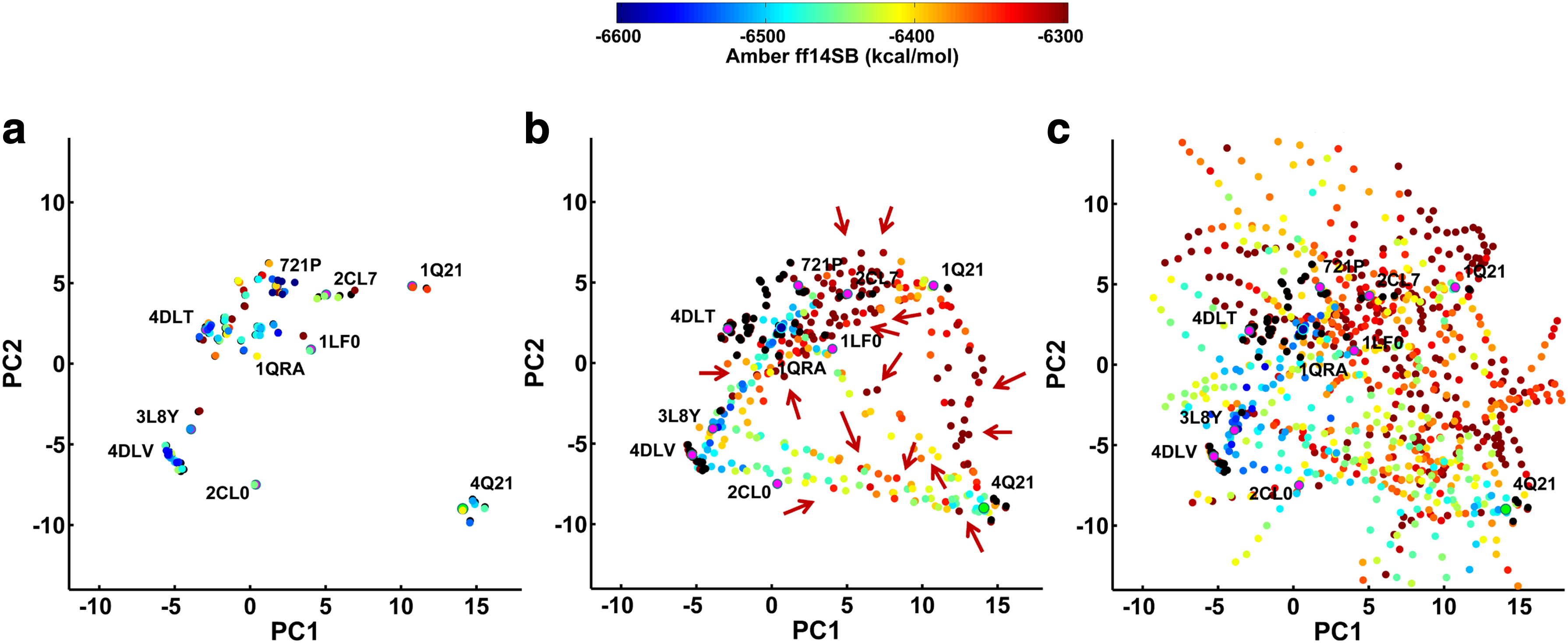
As related in Section 3.6.1, the population (cell counts) of each cell of the 2d grid (over PC1 and PC2) is recorded to obtain the density of state map for each algorithm. Cell width is set so that it corresponds to 1/50 of the maximum pairwise lRMSD among the experimentally known structures: 0.08 Å for H-Ras and 0.42 Å for CaM. Figure 2 color-codes cells by their population counts, using the same red-to-blue color-coding scheme for all three algorithms to indicate high-to-low cell counts. The left panel shows the results of the analysis for H-Ras, and the right panel does so for CaM. The exploration in SoPriM is concentrated on regions populated by the experimentally known structures that initialize its exploration. The exploitation bias in the initial population of known structure apportions away computational resources from exploration. This is particularly striking on CaM (right panel), where there are unpopulated regions separating those populated by known structures.

FIG. 2.

Grid cells are color-coded based on the number of samples per cell (color legend is shown at the top). Experimentally known structures are drawn as black dots.

In both proteins, SoPriMp yields more cells of high density; in particular, the regions missed by SoPriM on CaM are now populated. SoPriMo samples away from the known structures (as it explores directions that are orthogonal to those connecting the known structures). A direct quantitative comparison between SoPriMo and SoPriMp is facilitated by Table 1, where the number of populated cells not in regions containing experimentally known structures is juxtaposed to the number of cells populated by experimentally known structures. Table 1 shows that ordering by low to high exploration capability yields SoPriM, SoPriMp, and SoPriMo in the sorted order.

Table 1.

Number of Populated Cells Not Containing Experimentally Known Structures (New Cells) Versus Number of Cells Containing Experimentally Known Structures (Known Cells)

	Algorithm	No. of new cells	No. of known cells
H-Ras	SoPriM	28	240
	SoPriMp	36	87
	SoPriMo	36	44
CaM	SoPriM	34	98
	SoPriMp	40	81
	SoPriMo	43	56

4.1.2. Comparison of exploitation capability

We now compare the algorithms on their exploitation capability as described in Section 3.6. Figure 3 color-codes cells based on such differences, to show SoPriMp—SoPriM in the top row (the lowest energy reached by SoPriM in a cell is subtracted from the lowest energy reached by SoPriMp in the same cell), SoPriMo—SoPriM in the second row, and SoPriMo—SoPriMp in the third row. The left panel shows the comparisons for H-Ras, and the right panel does so for CaM. Cells with differences ≤10 kcal/mol are in light blue, those with differences in (−10, 10) kcal/mol are in gray, and those with differences ≥10 kcal/mol are in light pink. 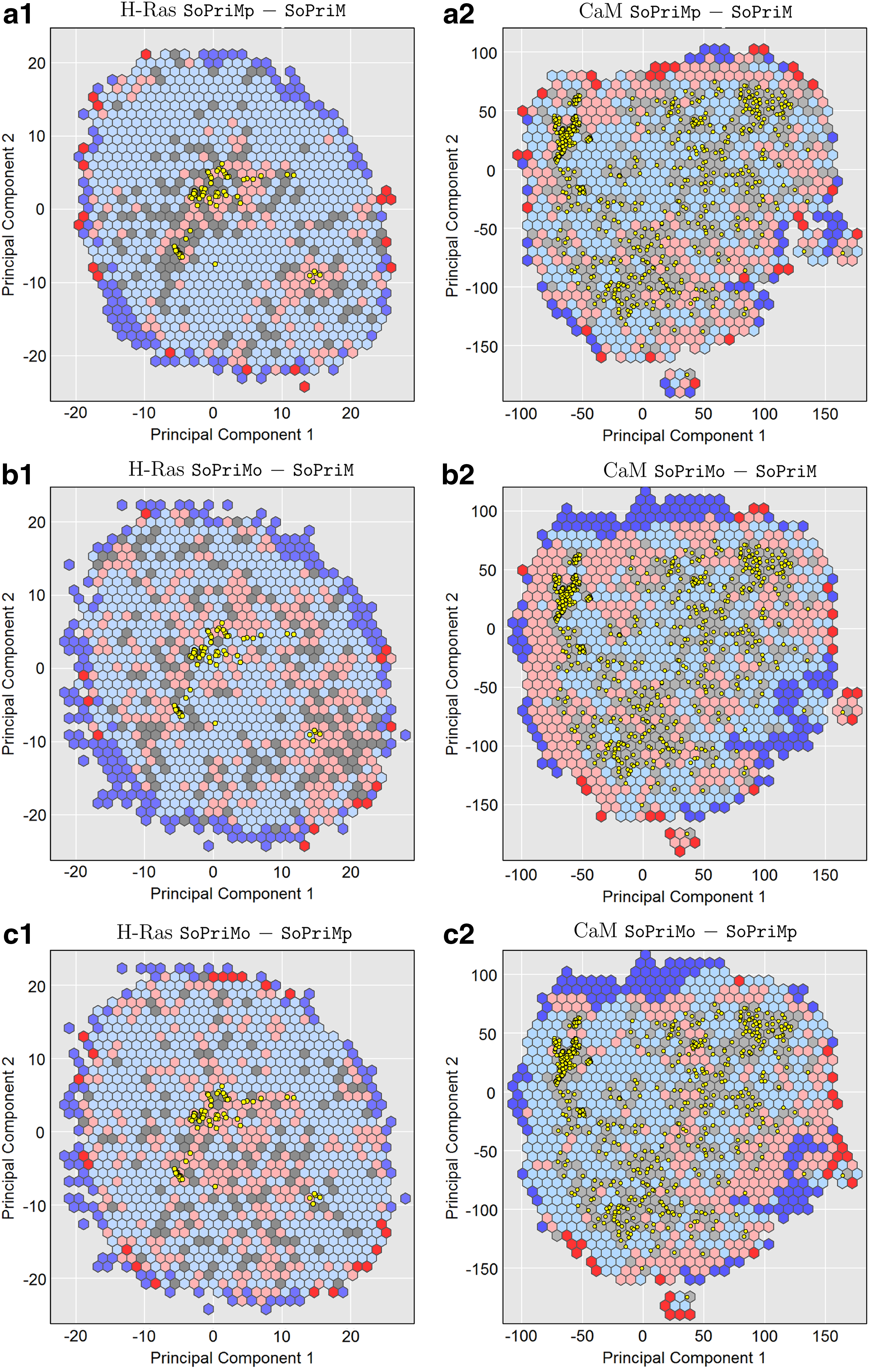In an A–B comparison, dark blue cells indicate those unpopulated by algorithm B, and dark red cells indicate those unpopulated by algorithm A. Projections of experimentally known structures are drawn as yellow dots.

FIG. 3.

Cells are colored based on the difference between the lowest-energy obtained in a cell by algorithm A and the lowest-energy obtained by algorithm B in that same cell. Cells with differences ≤10 kcal/mol are in light blue, (−10, 10) kcal/mol are in gray, and ≥10 kcal/mol are in light pink. Projections of experimentally known structures are drawn as yellow dots.

The exploitation maps for H-Ras in Figure 3a1–b1 suggest that both SoPriMp and SoPriMo populate the structure space with much lower-energy structures over SoPriM (more blue than pink cells). The only regions where SoPriM has more pink cells are those near the experimentally known structures that initialize it, as expected. These observations are supported by direct quantitative comparisons of counts of cells corresponding to the three categories of interest (lower, similar, or higher). Table 2 shows that on H-Ras, SoPriMp and SoPriMo populate 638/905 and 510/835 of the cells with lower-energy structures. These results make the case that on H-Ras, both SoPriMp and SoPriMo have higher exploitation capability than SoPriM.

Table 2.

Counts of 2d Hexagonal Cells with Different Categories of Lowest-Energy Differences

	Comparison	<	∼	>	Populated by both
H-Ras	SoPriMp–SoPriM	638	140	127	905
	SoPriMo–SoPriM	510	148	253	835
	SoPriMo–SoPriMp	599	119	256	974
CaM	SoPriMp–SoPriM	325	312	214	851
	SoPriMo–SoPriM	298	283	279	860
	SoPriMo–SoPriMp	380	282	213	875

CaM, calmodulin.

On CaM, the advantage of these two algorithms over SoPriM is smaller. Figure 3a2–b2 suggests that both SoPriMp and SoPriMo have higher exploitation capability over SoPriM, though not as pronounced as for H-Ras. The cell counts in Table 2 support these observations. On CaM, SoPriMp and SoPriMo populate a little more than a third of the cells with lower-energy structures over SoPriM and a little more two thirds of the cells with lower- or similar-energy structures over SoPriM. These results suggest that on vast configuration spaces (the CaM experimentally known structures span more than 10 Å in spatial scales), the differences may not be as stark; nonetheless, even in this challenging case, SoPriMp and SoPriMo achieve higher exploitation capability than SoPriM. The analysis also allows comparing SoPriMo with SoPriMp directly. Figure 3c1–c2 suggests that SoPriMo has higher exploitation capability than SoPriMp (more blue than pink cells). Table 2 shows that on H-Ras, SoPriMo populates 599/974 of the cells with lower energies than SoPriMp. On CaM, the advantage is less pronounced. SoPriMo populates 380/875 of the cells with lower energies than SoPriMp; the number of cells where both algorithms perform comparably is 282/875.

The results just cited confirm that ordering by low to high exploitation capability yields SoPriM, SoPriMp, and SoPriMo in the sorted order. This conclusion also holds when extending the analysis to 3d (building a grid with hexagonal cells over PC1-PC2-PC3; these three PCs capture more than 75% of the variance on both H-Ras and CaM). The plots that relate the differences between the algorithms are shown in Figure 4. The cell counts are related in Table 3.

FIG. 4.

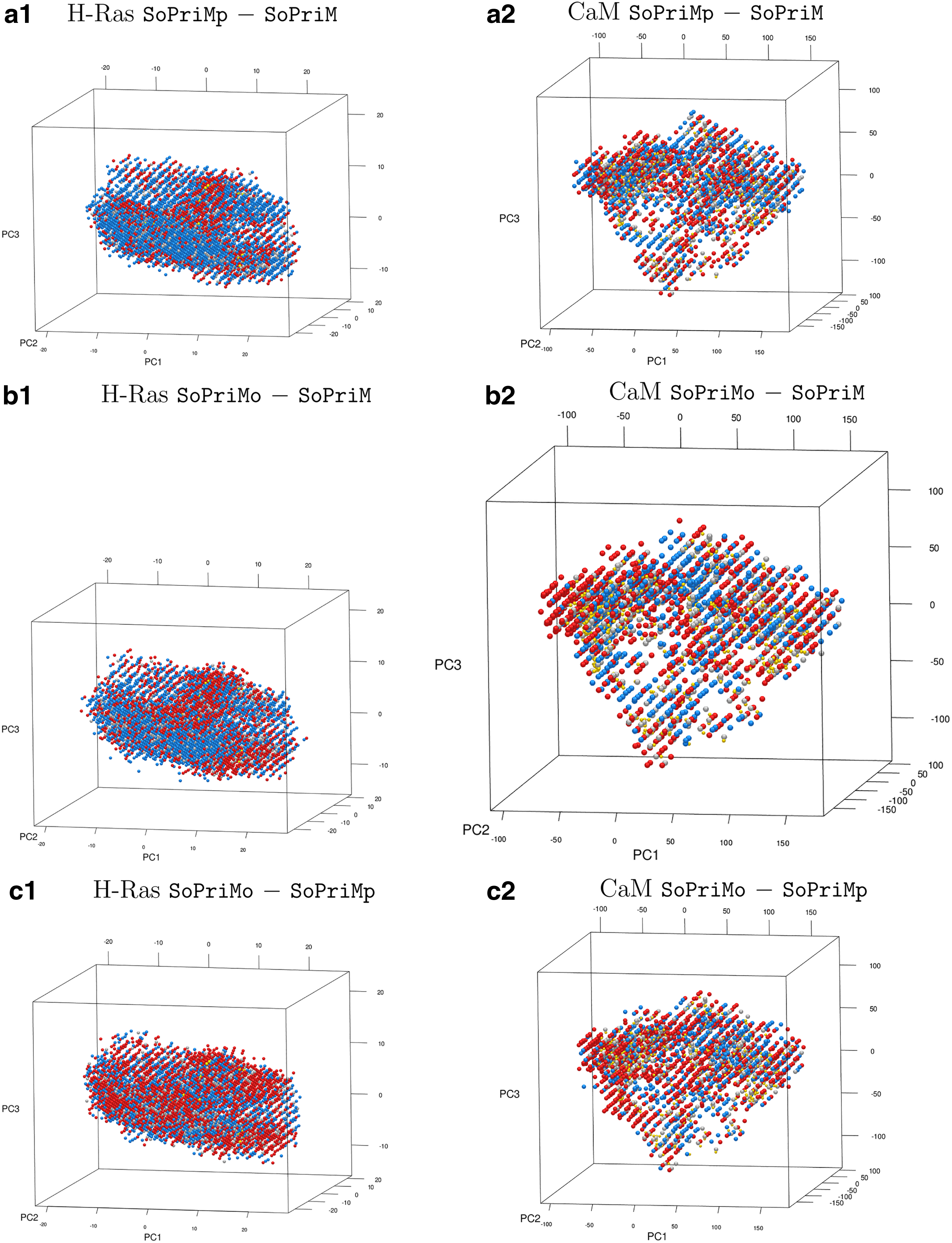
Grid cells are color-coded as in Figure 3. The grid is constructed over the top three PCs. Projections of experimentally known structures are drawn as yellow dots.

Table 3.

Counts of 3d Hexagonal Cells with Different Categories of Lowest-Energy Differences

	Comparison	<	∼	>	Populated by both
H-Ras	SoPriMp–SoPriM	2157	460	906	3523
	SoPriMo–SoPriM	1768	417	1330	3515
	SoPriMo–SoPriMp	1132	473	2008	3613
CaM	SoPriMp–SoPriM	801	441	782	2024
	SoPriMo–SoPriM	620	398	819	1837
	SoPriMo–SoPriMp	524	418	1007	1949

4.2. Comparison of lowest-cost paths

The algorithms are now compared on the quality of the lowest-cost path they find at different values r. On H-Ras, the structural rearrangement of interest here is the one that connects a representative structure of the active state (PDB identifier 1QRA) to representative of the inactive state (4Q21); note that r corresponds to the maximum allowed edge length. Table 4 shows that H-Ras sampling in SoPriM is not dense enough to be able to obtain a connected graph at values lower than 0.250 Å (no paths reported), whereas SoPriMo only fails at the lowest value of 0.1 Å.

Table 4.

Comparison of Lowest-Cost Paths at Varying r on Average and Median Edge Lengths \documentclass{aastex}\usepackage{amsbsy}\usepackage{amsfonts}\usepackage{amssymb}\usepackage{bm}\usepackage{mathrsfs}\usepackage{pifont}\usepackage{stmaryrd}\usepackage{textcomp}\usepackage{portland, xspace}\usepackage{amsmath, amsxtra}\usepackage{upgreek}\pagestyle{empty}\DeclareMathSizes{10}{9}{7}{6}\begin{document} $$( \langle el \rangle , \tilde el )$$ \end{document} , Average and Median Edge Costs ( \documentclass{aastex}\usepackage{amsbsy}\usepackage{amsfonts}\usepackage{amssymb}\usepackage{bm}\usepackage{mathrsfs}\usepackage{pifont}\usepackage{stmaryrd}\usepackage{textcomp}\usepackage{portland, xspace}\usepackage{amsmath, amsxtra}\usepackage{upgreek}\pagestyle{empty}\DeclareMathSizes{10}{9}{7}{6}\begin{document} $$\langle ec \rangle$$ \end{document} , \documentclass{aastex}\usepackage{amsbsy}\usepackage{amsfonts}\usepackage{amssymb}\usepackage{bm}\usepackage{mathrsfs}\usepackage{pifont}\usepackage{stmaryrd}\usepackage{textcomp}\usepackage{portland, xspace}\usepackage{amsmath, amsxtra}\usepackage{upgreek}\pagestyle{empty}\DeclareMathSizes{10}{9}{7}{6}\begin{document} $$\tilde ec$$ \end{document} ), Number of Vertices, and Path Cost

			Edge statistics
	r (Å)	Algorithm	\documentclass{aastex}\usepackage{amsbsy}\usepackage{amsfonts}\usepackage{amssymb}\usepackage{bm}\usepackage{mathrsfs}\usepackage{pifont}\usepackage{stmaryrd}\usepackage{textcomp}\usepackage{portland, xspace}\usepackage{amsmath, amsxtra}\usepackage{upgreek}\pagestyle{empty}\DeclareMathSizes{10}{9}{7}{6}\begin{document} $$\langle el \rangle$$ \end{document} , \documentclass{aastex}\usepackage{amsbsy}\usepackage{amsfonts}\usepackage{amssymb}\usepackage{bm}\usepackage{mathrsfs}\usepackage{pifont}\usepackage{stmaryrd}\usepackage{textcomp}\usepackage{portland, xspace}\usepackage{amsmath, amsxtra}\usepackage{upgreek}\pagestyle{empty}\DeclareMathSizes{10}{9}{7}{6}\begin{document} $$\tilde el$$ \end{document}	\documentclass{aastex}\usepackage{amsbsy}\usepackage{amsfonts}\usepackage{amssymb}\usepackage{bm}\usepackage{mathrsfs}\usepackage{pifont}\usepackage{stmaryrd}\usepackage{textcomp}\usepackage{portland, xspace}\usepackage{amsmath, amsxtra}\usepackage{upgreek}\pagestyle{empty}\DeclareMathSizes{10}{9}{7}{6}\begin{document} $$\langle ec \rangle$$ \end{document} , \documentclass{aastex}\usepackage{amsbsy}\usepackage{amsfonts}\usepackage{amssymb}\usepackage{bm}\usepackage{mathrsfs}\usepackage{pifont}\usepackage{stmaryrd}\usepackage{textcomp}\usepackage{portland, xspace}\usepackage{amsmath, amsxtra}\usepackage{upgreek}\pagestyle{empty}\DeclareMathSizes{10}{9}{7}{6}\begin{document} $$\tilde ec$$ \end{document}	No. of vertices	Cost
		SoPriM	0.14, 0.15	2.90, 6.37	31	129.92
	0.250	SoPriMp	0.17, 0.17	2.45, 3.17	28	83.61
		SoPriMo	0.19, 0.19	4.36, 4.60	20	84.44
H-Ras		SoPriMp	0.13, 0.14	1.51, 2.32	40	86.10
	0.201	SoPriMo	0.18, 0.17	1.89, 4.46	22	86.40
		SoPriMp	0.14, 0.14	1.63, 2.15	46	89.16
	0.167	SoPriMo	0.15, 0.14	2.41, 5.45	29	117.47
		SoPriMp	0.11, 0.11	2.52, 4.21	41	126.95
	0.124	SoPriMo	0.11, 0.11	5.26, 9.56	49	274.49
		SoPriMo	2.16, 1.69	261.37, 89.81	27	1354.55
	4.00	SoPriMp	0.80, 0.78	57.61, 12.27	30	837.00
		SoPriMo	1.04, 0.98	64.67, 10.76	25	777.61
		SoPriMp	0.83, 0.80	61.88, 13.69	28	837.00
	3.50	SoPriMo	1.01, 1.02	55.43, 10.79	29	777.61
CaM		SoPriMp	0.74, 0.77	66.23, 15.74	32	1028.16
	1.00	SoPriMo	0.78, 0.84	88.16, 11.99	26	1103.56
		SoPriMp	0.61, 0.64	72.06, 10.77	35	1226.54
	0.75	SoPriMo	0.62, 0.65	86.72, 18.02	31	1302.35
		SoPriMp	0.40, 0.41	162.26, 15.25	54	4301.51
	0.50	SoPriMo	0.41, 0.43	80.52, 19.60	53	2135.23
	0.42	SoPriMp	0.35, 0.37	134.68, 11.99	66	4378.53

Even when all algorithms report a path at a given value of r, the average and median edge lengths \documentclass{aastex}\usepackage{amsbsy}\usepackage{amsfonts}\usepackage{amssymb}\usepackage{bm}\usepackage{mathrsfs}\usepackage{pifont}\usepackage{stmaryrd}\usepackage{textcomp}\usepackage{portland, xspace}\usepackage{amsmath, amsxtra}\usepackage{upgreek}\pagestyle{empty}\DeclareMathSizes{10}{9}{7}{6}\begin{document} $$( \langle el \rangle , \tilde el )$$ \end{document} in SoPriM are higher than those in SoPriMp and SoPriMo, indicating sparser sampling in SoPriM. The average and median edge costs \documentclass{aastex}\usepackage{amsbsy}\usepackage{amsfonts}\usepackage{amssymb}\usepackage{bm}\usepackage{mathrsfs}\usepackage{pifont}\usepackage{stmaryrd}\usepackage{textcomp}\usepackage{portland, xspace}\usepackage{amsmath, amsxtra}\usepackage{upgreek}\pagestyle{empty}\DeclareMathSizes{10}{9}{7}{6}\begin{document} $$( \langle ec \rangle , \tilde ec )$$ \end{document} along the lowest-cost path are also higher in SoPriM over SoPriMp and SoPriMp at a given value of r, indicating that the better exploration and better exploitation in the latter two algorithms provide alternative routes with both shorter and lower-cost edges. Path costs initially go down at lower values of r, indicating a phase where lower-cost routes are found. Then, at the smallest values possible to find paths, as in 0.124 and 0.100 Å, the path cost goes up. Insisting that edges be short forces a path to go over small hills in the landscape, and thus follow the ruggedness much more closely, resulting in higher cost. Similar observations hold for CaM, supporting the conclusions that higher exploration and exploitation in sampling improve path quality, but that one should insist on higher sampling capability so that paths follow the landscape more closely.

4.3. Graphical statistical analysis of multi-dimensional energy landscapes

Prior work on SoPriM has validated some major energetic features (such as correspondence of visually identified basins with known long-lived structural states) for both H-Ras and CaM (Maximova et al., 2015, 2016c), but the analysis has been limited to visualizing color-coded PC1-PC2 projections of computed structures. Here, we make use of the conditioning technique described in Section 3.6.3 to extend the analysis from 2d to 4d landscapes.

4.3.1. Extracting biological insights from H-Ras multi-dimensional landscape

H-Ras is an enzyme that is central to human biology and is known to switch between different structures to regulate recognition of molecular partners. Structure switching spans 2.5 Å in all-atom lRMSD. Figure 5 relates the conditioned view of the 4d H-Ras energy landscape. The left top panel of Figure 5 (zoomed in to show the axes labels) shows a hexagonal bin plot along PC1 and PC2 conditioned on the first quartile of PC3 and the first quartile of PC4. The color scheme uses thresholds based on binned quantiles of cell minimum-energy distributions without subsetting. Quantiles of \documentclass{aastex}\usepackage{amsbsy}\usepackage{amsfonts}\usepackage{amssymb}\usepackage{bm}\usepackage{mathrsfs}\usepackage{pifont}\usepackage{stmaryrd}\usepackage{textcomp}\usepackage{portland, xspace}\usepackage{amsmath, amsxtra}\usepackage{upgreek}\pagestyle{empty}\DeclareMathSizes{10}{9}{7}{6}\begin{document} $$\{ 0 , 20 , 40 , 60 , 80 , 100 \} $$ \end{document} % correspond to Amber ff14SB energy values of \documentclass{aastex}\usepackage{amsbsy}\usepackage{amsfonts}\usepackage{amssymb}\usepackage{bm}\usepackage{mathrsfs}\usepackage{pifont}\usepackage{stmaryrd}\usepackage{textcomp}\usepackage{portland, xspace}\usepackage{amsmath, amsxtra}\usepackage{upgreek}\pagestyle{empty}\DeclareMathSizes{10}{9}{7}{6}\begin{document} $$\{ - 6703.342 ,$$ \end{document} \documentclass{aastex}\usepackage{amsbsy}\usepackage{amsfonts}\usepackage{amssymb}\usepackage{bm}\usepackage{mathrsfs}\usepackage{pifont}\usepackage{stmaryrd}\usepackage{textcomp}\usepackage{portland, xspace}\usepackage{amsmath, amsxtra}\usepackage{upgreek}\pagestyle{empty}\DeclareMathSizes{10}{9}{7}{6}\begin{document} $$- 6482.059 ,$$ \end{document} \documentclass{aastex}\usepackage{amsbsy}\usepackage{amsfonts}\usepackage{amssymb}\usepackage{bm}\usepackage{mathrsfs}\usepackage{pifont}\usepackage{stmaryrd}\usepackage{textcomp}\usepackage{portland, xspace}\usepackage{amsmath, amsxtra}\usepackage{upgreek}\pagestyle{empty}\DeclareMathSizes{10}{9}{7}{6}\begin{document} $$- 6430.048 ,$$ \end{document} \documentclass{aastex}\usepackage{amsbsy}\usepackage{amsfonts}\usepackage{amssymb}\usepackage{bm}\usepackage{mathrsfs}\usepackage{pifont}\usepackage{stmaryrd}\usepackage{textcomp}\usepackage{portland, xspace}\usepackage{amsmath, amsxtra}\usepackage{upgreek}\pagestyle{empty}\DeclareMathSizes{10}{9}{7}{6}\begin{document} $$- 6370.087$$ \end{document} , \documentclass{aastex}\usepackage{amsbsy}\usepackage{amsfonts}\usepackage{amssymb}\usepackage{bm}\usepackage{mathrsfs}\usepackage{pifont}\usepackage{stmaryrd}\usepackage{textcomp}\usepackage{portland, xspace}\usepackage{amsmath, amsxtra}\usepackage{upgreek}\pagestyle{empty}\DeclareMathSizes{10}{9}{7}{6}\begin{document} $$- 6291.812$$ \end{document} , \documentclass{aastex}\usepackage{amsbsy}\usepackage{amsfonts}\usepackage{amssymb}\usepackage{bm}\usepackage{mathrsfs}\usepackage{pifont}\usepackage{stmaryrd}\usepackage{textcomp}\usepackage{portland, xspace}\usepackage{amsmath, amsxtra}\usepackage{upgreek}\pagestyle{empty}\DeclareMathSizes{10}{9}{7}{6}\begin{document} $$- 4183.799 \} $$ \end{document} kcal/mol. The color scheme runs from dark to light blue, gray, and pink, using pink for the top three quantiles; yellow dots show projections of experimentally known structures.

FIG. 5.

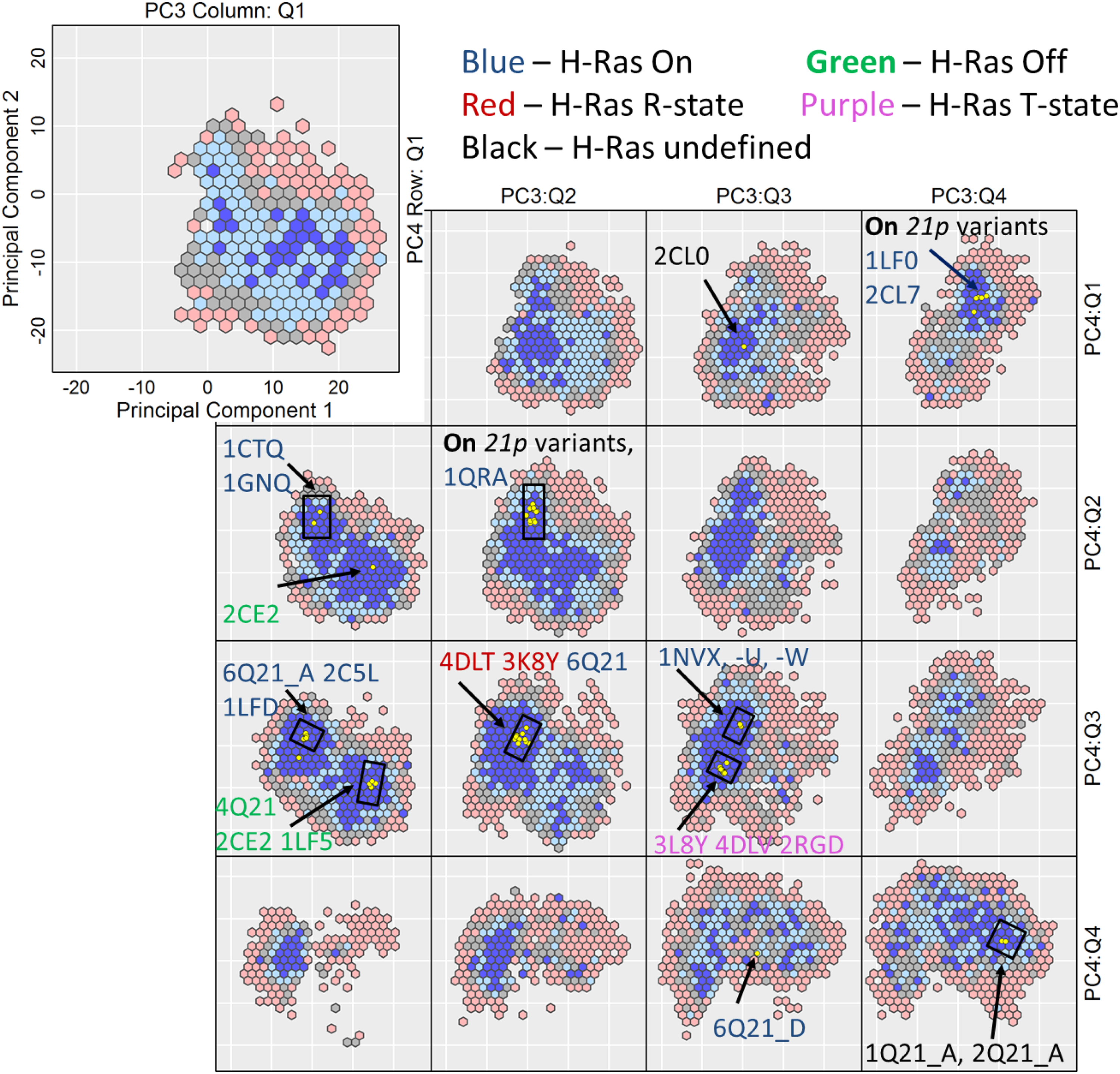
H-Ras: The 4d space in each subplot is discretized via hexagons, plotting for each only the projection of the lowest-energy structure. The blue-to-red color-coding scheme follows the low-to-high energy range. Yellow dots show projections of experimentally known structures.

By smoothing the ruggedness of the landscape, the hexagonal binning in the conditioned views allows seeing the distinct basins that correspond to the GTP- (active) and GDP-bound (inactive) states. The views that contain projections of experimentally known structures have been annotated with PDB ids of the known structures. The on and off basins corresponding to the active and inactive states, respectively, are most visible on the PC1-PC2 scatter plots along the first quartile of PC3 and the second (or third) quartile of PC4 (the [PC3:Q1, PC4:Q2–3] views). The [PC3:Q1, PC4:Q2–3] views show the barrier between the two basins. The R- and T-states are clearly part of the on basin (see the [PC3:Q2–3, PC4:3] views), supporting wet-laboratory evidence of allosteric switching in H-Ras (Buhrman et al., 2010; Johnson and Mattos, 2013). Both the on and off basins gradually disappear along the higher quartiles of PC3 and PC4, but the off basin persists along all quartiles of PC4, unlike the on basin (see [PC3:Q1, PC4:Q4]).

In addition, the experimentally known structures (based on their projections) appear on few (not all) quartiles of PC3 and PC4. There are specific regions of both the on and off basins that do not contain any experimentally known structures (see the [PC3:Q1, PC4:Q1,4], [PC3:Q2, PC4:Q1,4], [PC3:Q3,Q4, PC4:Q2], and [PC3:Q3, PC4:Q3] views). These constitute novel regions of the H-Ras landscape that have yet to be probed but are worth pursuing in wet laboratories, as they represent stable sub-states of possible interest for targeted therapeutic studies (Nussinov et al., 2014).

4.3.2. Extracting biological insights from CaM multi-dimensional landscape

CaM is also a functionally diverse enzyme of great importance to human biology. Structure switching in CaM spans over 20 Å in all-atom lRMSD. Figure 6 relates the conditioned view of the 4d CaM energy landscape. The color scheme is based on the quantiles \documentclass{aastex}\usepackage{amsbsy}\usepackage{amsfonts}\usepackage{amssymb}\usepackage{bm}\usepackage{mathrsfs}\usepackage{pifont}\usepackage{stmaryrd}\usepackage{textcomp}\usepackage{portland, xspace}\usepackage{amsmath, amsxtra}\usepackage{upgreek}\pagestyle{empty}\DeclareMathSizes{10}{9}{7}{6}\begin{document} $$\{ 0 , 20 , 40 , 60 , 80 , 100 \} $$ \end{document} %, which correspond to Amber ff14SB energy values of \documentclass{aastex}\usepackage{amsbsy}\usepackage{amsfonts}\usepackage{amssymb}\usepackage{bm}\usepackage{mathrsfs}\usepackage{pifont}\usepackage{stmaryrd}\usepackage{textcomp}\usepackage{portland, xspace}\usepackage{amsmath, amsxtra}\usepackage{upgreek}\pagestyle{empty}\DeclareMathSizes{10}{9}{7}{6}\begin{document} $$\{ - 5673.000$$ \end{document} , \documentclass{aastex}\usepackage{amsbsy}\usepackage{amsfonts}\usepackage{amssymb}\usepackage{bm}\usepackage{mathrsfs}\usepackage{pifont}\usepackage{stmaryrd}\usepackage{textcomp}\usepackage{portland, xspace}\usepackage{amsmath, amsxtra}\usepackage{upgreek}\pagestyle{empty}\DeclareMathSizes{10}{9}{7}{6}\begin{document} $$- 5066.380 ,$$ \end{document} \documentclass{aastex}\usepackage{amsbsy}\usepackage{amsfonts}\usepackage{amssymb}\usepackage{bm}\usepackage{mathrsfs}\usepackage{pifont}\usepackage{stmaryrd}\usepackage{textcomp}\usepackage{portland, xspace}\usepackage{amsmath, amsxtra}\usepackage{upgreek}\pagestyle{empty}\DeclareMathSizes{10}{9}{7}{6}\begin{document} $$- 4747.600$$ \end{document} , \documentclass{aastex}\usepackage{amsbsy}\usepackage{amsfonts}\usepackage{amssymb}\usepackage{bm}\usepackage{mathrsfs}\usepackage{pifont}\usepackage{stmaryrd}\usepackage{textcomp}\usepackage{portland, xspace}\usepackage{amsmath, amsxtra}\usepackage{upgreek}\pagestyle{empty}\DeclareMathSizes{10}{9}{7}{6}\begin{document} $$- 4493.720$$ \end{document} , \documentclass{aastex}\usepackage{amsbsy}\usepackage{amsfonts}\usepackage{amssymb}\usepackage{bm}\usepackage{mathrsfs}\usepackage{pifont}\usepackage{stmaryrd}\usepackage{textcomp}\usepackage{portland, xspace}\usepackage{amsmath, amsxtra}\usepackage{upgreek}\pagestyle{empty}\DeclareMathSizes{10}{9}{7}{6}\begin{document} $$- 4201.940$$ \end{document} , \documentclass{aastex}\usepackage{amsbsy}\usepackage{amsfonts}\usepackage{amssymb}\usepackage{bm}\usepackage{mathrsfs}\usepackage{pifont}\usepackage{stmaryrd}\usepackage{textcomp}\usepackage{portland, xspace}\usepackage{amsmath, amsxtra}\usepackage{upgreek}\pagestyle{empty}\DeclareMathSizes{10}{9}{7}{6}\begin{document} $$- 70.891 \} $$ \end{document} kcal/mol.

FIG. 6.

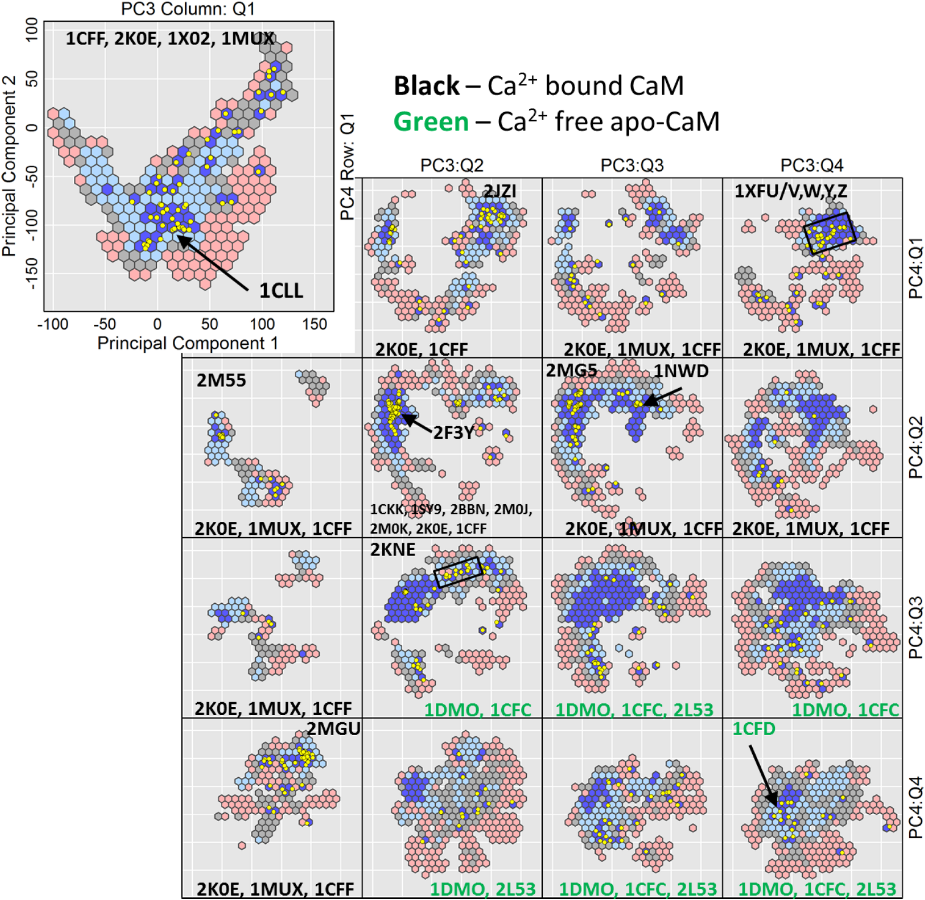
CaM: The 4d space in each subplot is discretized via hexagons, plotting for each only the projection of the lowest-energy structure. The blue-to-red color-coding scheme follows the low-to-high energy range. Yellow dots show projections of experimentally known structures. CaM, calmodulin.

As for H-Ras, several conditioned views show the absence of experimentally known structures in specific low-energy regions (see [PC3:Q2, PC4:Q4]), pointing to novel substates. The conditioned views contain precious information about possible structural rearrangements. In prior work, where we have analyzed the ability of SoPriM to compute lowest-cost paths connecting the calcium-bound state of CaM to the peptide/protein-bound state, we have shown that the lowest-cost path does not go through the calcium-free state (PDB ids 1CFC, 1CFD) (Maximova et al., 2016c). Indeed, tour calculations, where we calculate lowest-cost paths forced to go through specific structures, have shown that paths forced to go through the calcium-free state had higher costs.

The conditioned views in Figure 6 provide complementary insight into these structural rearrangements. The different views show that there are energy barriers that separate many of the small and large basins in the CaM landscape. As the PDB id annotations indicate in Figure 6, the conditioned views show that the calcium-bound and calcium-free open states group in specific regions of the energy landscape; the [PC3:Q1, PC4:Q1] view contains the calcium-bound open structures, whereas the [PC3:Q4, PC4:Q4] view contains the calcium-free open structures. Moreover, the calcium-free, open state of CaM is separated by energy barriers from the calcium-bound, closed state (see view [PC3:Q2, PC4:Q3]). These insights are in agreement with prior work (Maximova et al., 2016c). In summary, they indicate that CaM is able to switch between the calcium-bound closed and open states without releasing calcium ions, thus adding to the biological insight on structure-function mechanisms in CaM.

5. Discussion

This article demonstrates that a careful analysis of how each ingredient in a sample-based algorithm for modeling slow structural rearrangement affects exploration versus exploitation can result in novel design choices to improve both. The analysis demonstrates that novel initialization strategies, interleaved with exploration-driven selection mechanisms and exploitation-driven variation operator(s), improve both exploration and exploitation. Improvements in sampling translate to paths of higher granularity that follow the landscape more faithfully.

The questions posed and addressed in this article regarding sampling capability and its effect on the accuracy of modeled structural rearrangements are being raised among computational biophysicists embedding molecular structures obtained from many physics-based simulations in Markov state models (Gipson et al., 2012). The analysis and strategies proposed here to expose and address current limitations are a first step toward making sample-based models reliable tools for modeling slow structural rearrangements.

Detailed statistical analysis of multi-dimensional landscapes elucidates that sample-based models can yield novel insights regarding the structure-function relationship in two proteins that are of importance to human biology. The algorithms find stable regions not probed in the wet laboratory that may hold valuable information regarding druggability.

Footnotes

Acknowledgments

This work is supported in part by NSF SI2 No. 1440581 and NSF IIS CAREER Award No. 1144106. Computations were run on the ARGO research computing cluster at George Mason University.

Authors' Contributions

T.M., E. P., and A.S conceived the algorithm proposed here. T.M. implemented the algorithm and performed production runs. T.M. and A.S. conceived the experimental design. T.M., A.S., and D.C. conceived the data analysis strategy. T.M., Z.Z., and D.C. carried out the data analysis. T.M. and A.S. wrote the article.

Author Disclosure Statement

No competing financial interests exist.

References

Al-Bluwi

, Vaisset

, Siméon

, et al. 2013. Modeling protein conformational transitions by a combination of coarse-grained normal mode analysis and robotics-inspired methods. BMC Struct. Biol., 13(Suppl 1), S2.

Amaro

R.E.

, and Bansai

2014. Editorial overview: Theory and simulation: Tools for solving the insolvable. Curr. Opin. Struct. Biol., 25, 4–5.

Amato

N.M.

, Dill

K.A.

, and Song

2002. Using motion planning to map protein folding landscapes and analyze folding kinetics of known native structures. J. Comp. Biol., 10, 239–255.

Becker

O.M.

, and Karplus

1997. The topology of multidimensional potential energy surfaces: Theory and application to peptide structure and kinetics. J. Chem. Phys., 106, 1495–1517.

Berman

H.M.

, Henrick

, and Nakamura

2003. Announcing the worldwide Protein Data Bank. Nat. Struct. Biol. 10, 980.

Boehr

D.D.

, Nussinov

, and Wright

P.E.

2009. The role of dynamic conformational ensembles in biomolecular recognition. Nat. Chem. Biol., 5, 789–796.

Buhrman

, Holzapfel

, Fetics

, et al. 2010. Allosteric modulation of Ras positions Q61 for a direct role in catalysis. Proc. Natl. Acad. Sci. USA., 107, 4931–4936.

Carr

D.B.

1991. Looking at large data sets using binned data plots, 7–39. In Buja

, and Tukey

, eds. Computing and Graphics in Statistics. Springer-Verlag, New York, New York.

Carr

D.B.

1995. Scanning a 4-D domain for local minima: A protein folding example. Topics Sci. Vis., 6, 9–12.

10.

Carr

D.B.

, Nicholson

W.L.

, Littlefield

R.J.

, et al. 1986. Interactive color display methods for multivariate data, 215–250. In Wegman

E.J.

, and DePriest

D.J.

, eds. Statistical Image Processing and Graphics. Marcel Decker, New York, New York.

11.

Chiang

T.H.

, Apaydin

M.S.

, Brutlag

D.L.

, et al. 2007. Using stochastic roadmap simulation to predict experimental quantities in protein folding kinetics: Folding rates and phi-values. J. Comp. Biol., 14, 578–593.

12.

Choset

, et al. 2005. Principles of Robot Motion: Theory, Algorithms, and Implementations, 1st ed. MIT Press, Cambridge, MA.

13.

Clausen

, Ma

, Nussinov

, et al. 2015. Mapping the conformation space of wildtype and mutant h-ras with a memetic, cellular, and multiscale evolutionary algorithm. PLoS Comput. Biol. 11, e1004470.

14.

Clausen

, and Shehu

2015. A data-driven evolutionary algorithm for mapping multi-basin protein energy landscapes. J. Comp. Biol., 22, 844–860.

15.

Cleveland

W.S.

1993. Visualizing Data. Hobart Press, Summit, New Jersey.

16.

Dawkins

B.P.

1995. Investigating the geometry of a P-dimensional data sets. J. Amer. Stat. Assoc., 90, 350–359.

17.

Devaurs

, Molloy

, Vaisset

, et al. 2015. Characterizing energy landscapes of peptides using a combination of stochastic algorithms. IEEE Trans. Nanobioscience., 14, 545–552.

18.

Fischer

, and Karplus

1992. Conjugate peak refinement: An algorithm for finding reaction paths and accurate transition states in systems with many degrees of freedom. Chem. Phys. Lett., 194, 252–261.

19.

Gipson

, Hsu

, Kavraki

L.E.

, et al. 2012. Computational models of protein kinematics and dynamics: Beyond simulation. Annu. Rev. Anal. Chem., 5, 273–291.

20.

Haspel

, Moll

, Baker

M.L.

, et al. 2010. Tracing conformational changes in proteins. BMC Struct. Biol., 10(Suppl 1), S1.

21.

Jaillet

, Corcho

F.J.

, Perez

J.-J.

, et al. 2011. Randomized tree construction algorithm to explore energy landscapes. J. Comput. Chem., 32, 3464–3474.

22.

Jaillet

, Cortés

, and Siméon

2008. Transition-based RRT for path planning in continuous cost spaces, 22–26. In IEEE/RSJ International Conference on Intelligent Robots and Systems. AAAI, Stanford, CA.

23.

Johnson

C.W.

, and Mattos

2013. The allosteric switch and conformational states in ras GTPase affected by small molecules. Enzymes. 33(Pt. A), 41–67.

24.

Krivov

G.G.

, Shapovalov

M.V.

, and Dunbrack

R.L.

Jr.

2009. Improved prediction of protein side-chain conformations with SCWRL4. Proteins. 77, 778–795.

25.

Maier

J.A.

, Martinez

, Kasavajhala

, et al. 2015. ff14SB: Improving the accuracy of protein side chain and backbone parameters from ff99SB. J. Chem. Theor. Comput., 11, 3696–3713.

26.

Maximova

, Carr

, Plaku

, et al. 2016a. Sample-based models of protein structural transitions, 128–137. In Conference on Bioinformatics and Computational Biology (BCB). ACM, Seattle, WA. Editors: Shi

, and Shen

27.

Maximova

, Moffatt

, Ma

, et al. 2016b. Principles and overview of sampling methods for modeling macromolecular structure and dynamics. PLoS Comp. Biol., 12, e1004619.

28.

Maximova

, Plaku

, and Shehu

2015. Computing transition paths in multiple-basin proteins with a probabilistic roadmap algorithm guided by structure data, 35–42. In Intelligent Conference on Bioinformatics and Biomedicine. IEEE, Washington, D.C. Editors: Ning

, and Jiang

29.

Maximova

, Plaku

, and Shehu

2016c. Structure-guided protein transition modeling with a probabilistic roadmap algorithm. IEEE/ACM Trans. Bioinf. Comp. Biol., 13, 1–14.

30.

Molloy

, Clausen

, and Shehu

2016. A stochastic roadmap method to model protein structural transitions. Robotica. 34, 1705–1733.

31.

Molloy

, Saleh

, and Shehu

2013. Probabilistic search and energy guidance for biased decoy sampling in ab-initio protein structure prediction. IEEE/ACM Trans. Bioinf. Comp. Biol., 10, 1162–1175.

32.

Molloy

, and Shehu

2013. Elucidating the ensemble of functionally-relevant transitions in protein systems with a robotics-inspired method. BMC Struct. Biol., 13(Suppl 1), S8.

33.

Molloy

, and Shehu

2015. Interleaving global and local search for protein motion computation, 175–186. In Harrison

, Li

, and Mandoiu

, eds. LNCS: Bioinformatics Research and Applications, volume 9096. Springer International Publishing, Norfolk, VA.

34.

Molloy

, and Shehu

2016. A general, adaptive, roadmap-based algorithm for protein motion computation. IEEE Trans. Nanobioscience, 2, 158–165.

35.

Nussinov

, Jang

, and Tsai

C.-J.

2014. The structural basis for cancer treatment decisions. Oncotarget. 5, 7285–7302.

36.

Nussinov

, and Wolynes

P.G.

2014. A second molecular biology revolution? the energy landscapes of biomolecular function. Phys. Chem. Chem. Phys., 16, 6321–6322.

37.

Okazaki

, Koga

, Takada

, et al. 2006. Multiple-basin energy landscapes for large-amplitude conformational motions of proteins: Structure-based molecular dynamics simulations. Proc. Natl. Acad. Sci. USA., 103, 11844–11849.

38.

Olson

, Hashmi

, Molloy

, et al. 2012. Basin hopping as a general and versatile optimization framework for the characterization of biological macromolecules. Adv. Artif. Intell. J. 674832.

39.

Russel

, et al. 2009. The structural dynamics of macromolecular processes. Curr. Opin. Cell. Biol., 21, 97–108.

40.

Shehu

Conformational search for the protein native state. In Rangwala

, and Karypis

, eds. Protein Structure Prediction: Method and Algorithms, chapter 21. Wiley Book Series on Bioinformatics, Fairfax, VA, 2010.

41.

Shehu

Probabilistic search and optimization for protein energy landscapes. In Aluru

, and Singh

, eds. Handbook of Computational Molecular Biology. Chapman & Hall/CRC Computer & Information Science Series, 2013, Boca Raton, FL.

42.

Shehu

, and Olson

2010. Guiding the search for native-like protein conformations with an ab-initio tree-based exploration. Intl. J. Robot. Res., 29, 1106–1127.

43.

Shehu

, and Plaku

2016. A survey of omputational treatments of biomolecules by robotics-inspired methods modeling equilibrium structure and dynamics. J. Artif. Intell. Res., 597, 509–572.

44.

Singh

A.P.

, Latombe

J.-C.

, and Brutlag

D.L.

1999. A motion planning approach to flexible ligand binding, 252–261. In Schneider

, Bork

, Brutlag

D.L.

, Glasgow

J.I.

, Mewes

H.-W.

, and Zimmer

, eds. Proceedings of International Conference on Intelligent Systems for Molecular Biology (ISMB), volume 7. AAAI, Heidelberg, Germany.

45.

Tang

, Thomas

, Tapia

, et al. 2008. Simulating rna folding kinetics on approximated energy landscapes. J. Mol. Biol., 381, 1055–1067.

46.

Tapia

, Tang

, Thomas

et al. 2007. Kinetics analysis methods for approximate folding landscapes. Bioinformatics. 23, i539–i548.

47.

Tapia

, Thomas

and Amato

2010. A motion planning approach to studying molecular motions. Commun. Inf. Sys., 10, 53–68.

48.

Thomas

, Song

, and Amato

N.M.

2005. Protein folding by motion planning. J. Phys. Biol. 2, 148.

49.

Thomas

, Tang

, Tapia

, et al. 2007. Amato. Simulating protein motions with rigidity analysis. J. Comput. Biol., 14, 839–855.