Viral Capsid Assembly: A Quantified Uncertainty Approach

Abstract

Most of the existing research in assembly pathway prediction/analysis of viral capsids makes the simplifying assumption that the configuration of the intermediate states can be extracted directly from the final configuration of the entire capsid. This assumption does not take into account the conformational changes of the constituent proteins as well as minor changes to the binding interfaces that continue throughout the assembly process until stabilization. This article presents a statistical-ensemble-based approach that samples the configurational space for each monomer with the relative local orientation between monomers, to capture the uncertainties in binding and conformations. Further, instead of using larger capsomers (trimers, pentamers) as building blocks, we allow all possible subassemblies to bind in all possible combinations. We represent the resulting assembly graph in two different ways: First, we use the Wilcoxon signed-rank measure to compare the distributions of binding free energy computed on the sampled conformations to predict likely pathways. Second, we represent chemical equilibrium aspects of the transitions as a Bayesian Factor graph where both associations and dissociations are modeled based on concentrations and the binding free energies. We applied these protocols on the feline panleukopenia virus and the Nudaurelia capensis virus. Results from these experiments showed a significant departure from those that one would obtain if only the static configurations of the proteins were considered. Hence, we establish the importance of an uncertainty-aware protocol for pathway analysis, and we provide a statistical framework as an important first step toward assembly pathway prediction with high statistical confidence.

1. Introduction

Viruses are the smallest living organisms on earth, possessing only a minimal genome that can transcribe only a few proteins. Even with such limited resources, viruses exhibit a remarkable ability to not only survive but also parasitically multiply with great efficiency. One phase of their chemical proliferation that is relatively unexplained is the spontaneous assembly/disassembly of hundreds of (capsid) proteins that come together to form the capsid (shell) that encases the viral nucleic acid genetic material. Researchers continue to analyze this remarkable process from different perspectives, and they also aim at using the insights discovered in designing nano-scale cages and shells for drug delivery (Cheng et al., 2008; Zochowska et al., 2009; Lai et al., 2013; Smith et al., 2013). In this article, we present a statistical methodology to analyze the viral assembly process from a free energy perspective. We consider in particular two cases: the feline panleukopenia virus (PDBID:1C8F) (Simpson et al., 2000) and the Nudaurelia capensis virus (PDBID:1OHF) (Helgstrand et al., 2004). Although others have taken a similar perspective earlier (Zlotnick, 1994; Rapaport et al., 1999; Hagan and Chandler, 2006; Zlotnick and Mukhopadhyay, 2011; Hagan, 2014), we are the first to consider positional and conformational uncertainties of the protein structure and their propagated influence on the configurational energetics and binding affinity calculations. This methodology then allows us to infer energetically favorable viral capsomer configurations and assembly pathways, together with improved statistical confidence.

Research at understanding the assembled arrangement of capsid proteins in a viral capsid builds on the work of Caspar and Klug (C-K) (Caspar and Klug, 1962). C-K characterize the symmetric organization of proteins in a spherical viral capsid, building on the mathematical foundations of spherical tilings given by Goldberg (1937). C-K show that the combinatorial arrangement of the capsid proteins can be characterized by using simple triangular tiles, each tile consisting of three copies of the protein (a trimer), that cover an icosahedron. Essentially, the entire capsid can be considered as 20T trimers; or as 12 pentamers and 10(T − 1) examers. This concept, called “quasi-equivalence,” states that all the viral protein chains that form a capsid are identical and have (quasi-) equivalent interfaces—essentially, all proteins are involved in the same number of interactions at similar binding sites.

Recent work (Janner, 2006; Keef and Twarock, 2009) has shown that certain aperiodic arrangements involving pentamers or other types of subassemblies are also possible. Other work (Pawley, 1961) has shown that several other symmetry classes also permit decomposition into symmetric subassemblies, and Rasheed and Bajaj (2015) proved necessary and sufficient conditions for such subassemblies to be possible. Brooks and colleagues, in a series of papers, have characterized the geometric conditions for symmetric capsids, provided methods to measure how much a specific capsid conforms to the concept of quasi-equivalence (Damodaran et al., 2002; Carrillo-Tripp et al., 2008; Mannige and Brooks, 2008), and hence how amenable it is to coarse-grained dynamics analysis as described later. Further, they present a simple classification that characterizes variations of hexamers within a capsid (Mannige and Brooks, 2010).

Many of the researchers working on predicting, analyzing, and/or simulating capsid assembly have taken either a set of trimers or a set of pentamers+hexamers as the building blocks of assembly. For instance, Rapaport et al. (1999) performed a coarse dynamics simulation where trimers were used as building blocks. It successfully showed that even simple shape and binding site conditions are sufficient to drive self-assembly. In their more recent work (Rapaport, 2004, 2010), the model was updated to include more complex energetics, and single proteins (monomers) were used as building blocks, instead of trimers.

Hagan et al. (Hagan and Chandler, 2006; Elrad and Hagan, 2008) applied Brownian dynamics simulation with a simplified force field. They modeled each capsomer (which can also be a monomer) by using a single bead model. Based on prior knowledge about the arrangement of such beads on the capsid, they parametrized each bead based on the angles between each pair of their neighbors, and designed a binding affinity function that allowed binding at specific orientations. This concept is similar to the “local-rules” introduced by Berger et al. (Berger and Shor, 1994; Berger et al., 1994), which has been adopted by other groups (Schwartz et al., 1998; Xie et al., 2012) for kinetics and dynamics analysis of capsids. A discussion contrasting the block-like beads used by Rapaport et al. with shape-driven assembly, and the ones used by Hagan et al. with neighborhood-driven assembly can be found in Hagan (2014). Bona and Sitharam also considered a bead-like model (Bona et al., 2011); however, they modeled the interaction of the beads by using geometric stability conditions and predicted the likelihood of binding based on the simplicity of solving the geometric constraints system (Sitharam et al., 2004).

Unlike the dynamics-based analysis techniques described earlier, Zlotnick (1994) applied the statistical thermodynamics law of mass action to relate the concentrations of the constituents and the product of a binding with the binding free energy. Using pentameric building blocks, he enumerated all unique compositions of one or more pentamers (each arranged exactly as it would be if the entire capsid was formed). This technique, and several following publications (Zlotnick, 2005, 2006), revealed various aspects of assembly for different viruses, including rates of assembly, effect of nucleation, detection of possible kinetic traps, etc. It also provided a simple tool to predict the effect of changing environment parameters and/or presence of other molecules, which can be applied to measure yields under different conditions, designing conditions that are amenable to specific assemblies, etc. (Burns et al., 2009; Zlotnick and Mukhopadhyay, 2011).

This article presents an approach to score and rank conformational ensembles of capsid protein capsomers and capsid subassemblies based on a new configurational sampling and energy analysis approach. The sampled configurations of capsid subassemblies represent the various potential intermediate states of a fully assembled viral capsid. In other words, we recognize that the tertiary structure (fold) of individual subunits as well as binding contacts between subunits may evolve over the span of the entire assembly process, and moreover, may exist in slightly different configurations for the same subassemblies. The presence of such uncertainties implies that any binding free energy computed solely based on the structure and interfaces that exist in the final matured state of the capsid is not always accurate. Similar uncertainty quantification and uncertainty propagation methods have recently been used for single-molecule models (Lei et al., 2014; Rasheed et al., 2015) but not for combinatorial arrangements of viral capsid proteins in various capsomeric states.

In our approach, given prior knowledge (in the form of statistical distributions) of the nature of uncertainty, we can provide additional theoretical upper bounds on the distributional moments (Hoeffding, 1963; Azuma, 1967; McDiarmid, 1989) for different properties of viral capsomers, and other quantities of interest (QOI, e.g., the binding free energy). (See for, e.g., Rasheed et al. (2015) for such Azuma-Hoeffding bounds applied to molecular modeling with atomistic positional uncertainty captured by B-factors.) In addition, if the space of configurations is sampled such that low discrepancy (and also low dispersion) is achieved, then a probability distribution of the QOI can be approximated with bounded error (Niederreiter, 1990; Hoogland et al., 1998). Such estimation of binding free energies, that is, as distributions instead of single values, makes it possible to sample energy landscapes through various configurational ensembles, and to analyze binding pathways in an efficient and robust way (Rasheed et al., 2015). We apply our efficient low-discrepancy product-space sampling technique reported in Bajaj et al. (2014) to generate such low-discrepancy sampled ensembles of viral capsomers. The configuration space for any subassembly of the capsid is a product space of the backbone torsion angles between relatively rigid domains, as well as three-dimensional affine transformations between each pair of neighbors.

We construct an assembly pathway graph consisting of all possible state transitions, and we define a Bayesian factor graph parameterized based on the distributions of binding free energies. The state transitions are designed to capture the effect of the binding free energy and the concentration of the constituents under equilibrium (similar to Zlotnick, 1994). This provides a robust approach to predicting and analyzing stable assembly pathways, and to predicting concentrations of all subassemblies, with quantified uncertainty.

1.1. Differences from the CSBW16 version

The findings reported in this article were originally published in the Computational Structural Bioinformatics Workshop (CSBW’16), held in conjunction with IEEE BIBM. In this JCB special issue version of the article, we have expanded on our presentation of the materials and methods for enhanced clarity. In particular, Section 2.1 has been expanded for clarity; seven paragraphs have been added under Section 2.2.2 with a heading “Sampling the configurational space of capsid assembly,” which exposes the application of sampling algorithms specifically for the viral capsid assembly space. A new section (Section 3.1) has been added, which establishes that the number of samples used to model each assembly state was sufficient. Further, Sections 3.3 and 3.4 describe a statistical ranking procedure and corresponding results for identifying likely subassemblies and pathways. We also report extended results on the N. capensis virus (PDBID:1OHF) (Helgstrand et al., 2004). In addition, we analyzed the capsid assembly of the feline panleukopenia virus (PDBID:1C8F) (Simpson et al., 2000), and showcases when this new capsid exhibits assembly behavior departing from intuition. Several new figures (Fig. 2, Fig. 3e–h, Figs. 4 –6, Fig. 8, Fig. 12b, and Fig. 13b) and an additional table (Table 1) have been added.

Table 1.

Number of Samples Needed to Reach Saturation Across All Samples for Both PDBID:1OHF and PDBID:1C8F, Using Total Free Energy as Measured Statistic

No. of samples needed for saturation	% 1OHF	% 1C8F
\documentclass{aastex}\usepackage{amsbsy}\usepackage{amsfonts}\usepackage{amssymb}\usepackage{bm}\usepackage{mathrsfs}\usepackage{pifont}\usepackage{stmaryrd}\usepackage{textcomp}\usepackage{portland, xspace}\usepackage{amsmath, amsxtra}\usepackage{upgreek}\pagestyle{empty}\DeclareMathSizes{10}{9}{7}{6}\begin{document} $$<$$ \end{document} 100	2.6	0.0
100–200	39.9	92.5
200–300	26.0	7.5
300–400	10.3	0.0
400–500	7.7	0.0
500–600	3.3	0.0
600–700	3.2	0.0
700–800	2.3	0.0
900–900	2.2	0.0
900–950	1.2	0.0
950–975	1.2	0.0
>975	0.0	0.0

Number of samples defined by Chernoff-like bounds for incremental sampling approach. Most of the subassemblies require fewer than 500 samples; only 1 of the subassemblies in either capsid required more than 900 samples.

2. Methods

One of the major goals of this work is to develop a method for viral self-assembly pathway analysis with statistical guarantees. We consider assembly from an equilibrium perspective, where, given prior knowledge of the final assembled structure, we can uniquely determine the possible subassemblies of different sizes and the possible ways they can be associated/disassociated. We assume, similar to the work of Zlotnick et al. (Zlotnick, 1994, 2005; Zlotnick, 2006; Burns et al., 2009; Zlotnick and Mukhopadhyay, 2011), that the binding free energy of the association governs the success and yield of the reaction. However, we apply a more robust estimation of the binding energy under an uncertainty quantification framework. In addition, we consider all possible assembly pathways starting from monomers, instead of assuming that trimers, pentamers, etc. are the basic building blocks.

The overall methodology for this research is as follows. First, we identify all unique interfaces and unique subassemblies of specific sizes (where “size” is defined as the number of constituent monomers) of a given virus. Second, we sample the space of configurations for each of these subassemblies with restricted range of motion to generate an ensemble of structures in an attempt to capture the uncertainty (flexibility, random perturbations, etc.) of the structure. Then, we compute the free energy of each sample of each subassembly to generate a distribution of the energy. Finally, we use these distributions of energies (instead of the traditional single value) to compare the stabilities of the subassemblies, model state transition, and concentrations by using a probabilistic factor graph representation, and we derive statistical predictions on likely pathways. In the following subsections, we discuss each of these in detail.

2.1. Unique subassemblies and transitions

Analysis of self-assembly focusing on only a predetermined set of pathways fails to take into account subassemblies caught into energy traps, which, nonetheless, may be part of a pathway that is globally favorable to the capsid as a whole (Hagan and Chandler, 2006; Elrad and Hagan, 2008). For this reason, we have sought to implement an exhaustive approach. We consider all possible unique subassemblies and all possible pathways for these subassemblies to be formed.

To begin, we consider each chain to be unique. Even though the chains have the same primary structure, in most cases they exhibit minor differences in their tertiary configuration and, hence, it is preferable to consider each of them as unique—especially when computing binding free energies. For subassemblies involving two or more monomers, we consider them to be equivalent if and only if all three following conditions (evaluated in this order) are met: (1) They have the same number of monomers of each type, (2) they have the same number of symmetric interfaces of each type, and (3) when the atoms of both subassemblies are aligned, the root mean square distance (RMSD) is small.

For example, the N. capensis virus (PDBID:1OHF) has 240 proteins on its capsid, and it has four unique monomers: A, B, C, and D. It has several unique symmetric interfaces, with each appearing multiple times on the capsid. In Figure 1, we show a portion of capsid where each of these unique interface types is present at least once. For example, fivefold between A1-A2, A2-A3, etc.; sixfold between C1-B5, B5-D5, C1-D7, etc; threefold between A1-B1, A1-C1, B1-C1, D1-D7, etc.; and twofold between C1-D1, A1-B5, etc. According to our criterion, A1-B1 and A5-B5 are equivalent to each other but not equivalent to A1-B5 (violates criterion 2). A4-A5-A1-B5 is equivalent to A5-A1-A2-B1 but distinct from A1-A2-A3-B1 (violates criterion 3). The panleukopenia virus (PDBID:1C8F; Fig. 2) contains 60 proteins on its capsid, with all proteins arising from the same genetic sequence. Even though this protein contains fewer monomers than the N. capensis capsid, the intertwining nature of the protein interface provides additional interfaces that would not otherwise be available, such as the repeated interface between A1 and A6.

FIG. 1.

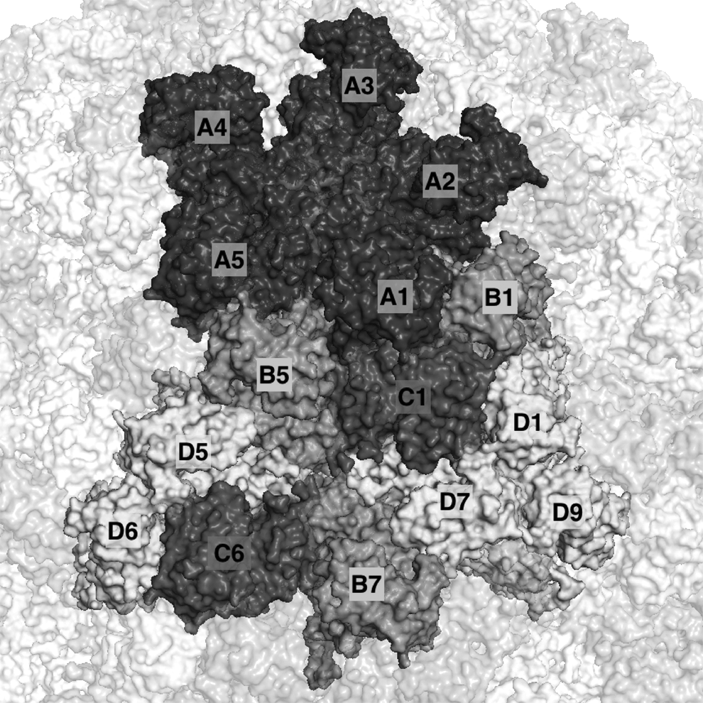
A portion of the Nudaurelia capensis virus capsid (PDBID:1OHF). Labels on the capsid show individual monomeric capsid proteins of different types (A, B, C, or D), at different locations, forming different local subassemblies. For instance, the capsomer A1-A2-A3-A4-A5 forms a pentameric configuration and contains four 5-fold interfaces of the same type. Similarly, A1-B1-C1 and D1-D7-D9 are two trimers, but they involve slightly different interfaces.

FIG. 2.

A portion of the feline panleukopenia virus capsid (PDBID:1C8F). Labels on the capsid shows individual monomeric subunits at different locations. Since all subunits are composed of the same sequence, each monomer is colored different. Capsomer A1-A2-A3-A4-A5 forms a pentameric configuration and contains four 5-fold interfaces of the same type. Also present is the trimeric interface between A1-A7-A9 and the dimeric interfaces between A1-A6 and A1-A7.

We select a set of subassemblies such that no member of the set is equivalent to any other member. For the N. capensis virus, this resulted in 985 unique subassemblies involving up to six monomers. This set includes some of the more distinct capsomers of this capsid: the trimers (A1-B1-C1) and (D1-D7-D9), the pentamer (A1-A2-A3-A4-A5), and the hexamer (B5-C1-D7-B7-C6-D5). There were 199 unique subassemblies for the panleukopenia virus.

We consider a transition from subassembly P to subassembly Q feasible if it is possible to add one monomer to P to make it equivalent to Q. For example, for the case shown in Figure 1, (A1-B1-C1) is reachable from (A1-B1), (B1-C1), and (A1-C1).

2.2. Sampling of subassemblies

As mentioned earlier, instead of considering a static model for a subassembly, we are interested in modeling subassemblies as a distribution of possible structures that have minor differences, but represent the same state. One way to think of this is to consider an energy well that contains the specific subassembly and many others that are just slightly different—in such case, one should not focus on only one of them to characterize the well, but should consider the entire distribution. In this regard, we consider both small changes inside subunit conformation (the natural shift in structure of the protein backbone) and slight perturbations of the interface. We now describe a parameterization of these spaces.

2.2.1. Configuration space of a subassembly

Although, in principle, backbone torsional angles are all relevant for internal flexibility of a protein, for the sake of tractability (especially for the multitude of subassemblies of the capsid), we applied a coarse-grained approach based on domain decomposition. We limited the sampling space to flexible backbone torsion angles between relatively rigid subdomains. To determine the set of flexible backbone torsion angles, we used HingeProt (Emekli et al., 2008) to identify hinge residues, designating the corresponding \documentclass{aastex}\usepackage{amsbsy}\usepackage{amsfonts}\usepackage{amssymb}\usepackage{bm}\usepackage{mathrsfs}\usepackage{pifont}\usepackage{stmaryrd}\usepackage{textcomp}\usepackage{portland, xspace}\usepackage{amsmath, amsxtra}\usepackage{upgreek}\pagestyle{empty}\DeclareMathSizes{10}{9}{7}{6}\begin{document} $$\phi$$ \end{document} and \documentclass{aastex}\usepackage{amsbsy}\usepackage{amsfonts}\usepackage{amssymb}\usepackage{bm}\usepackage{mathrsfs}\usepackage{pifont}\usepackage{stmaryrd}\usepackage{textcomp}\usepackage{portland, xspace}\usepackage{amsmath, amsxtra}\usepackage{upgreek}\pagestyle{empty}\DeclareMathSizes{10}{9}{7}{6}\begin{document} $$\psi$$ \end{document} internal torsion angles of each residue as flexible (i.e., if there were r hinge residues, there were a total of 2r rotatable bonds). This results in a configurational space equivalent to \documentclass{aastex}\usepackage{amsbsy}\usepackage{amsfonts}\usepackage{amssymb}\usepackage{bm}\usepackage{mathrsfs}\usepackage{pifont}\usepackage{stmaryrd}\usepackage{textcomp}\usepackage{portland, xspace}\usepackage{amsmath, amsxtra}\usepackage{upgreek}\pagestyle{empty}\DeclareMathSizes{10}{9}{7}{6}\begin{document} $${ {\mathbb{R}}^{2r}}$$ \end{document} .

We parametrize the space of local affine perturbations of each pairwise interface between every pair of monomers in a subassembly by using 6 degrees of freedom, defined by three Euler angle twists and three translational shifts. Hence, for a subassembly with t pairwise interfaces, the space is equivalent to \documentclass{aastex}\usepackage{amsbsy}\usepackage{amsfonts}\usepackage{amssymb}\usepackage{bm}\usepackage{mathrsfs}\usepackage{pifont}\usepackage{stmaryrd}\usepackage{textcomp}\usepackage{portland, xspace}\usepackage{amsmath, amsxtra}\usepackage{upgreek}\pagestyle{empty}\DeclareMathSizes{10}{9}{7}{6}\begin{document} $${{ \mathbb{R}}^{6t}}$$ \end{document} .

2.2.2. Sampling

Recall that we want to estimate the distribution of free energy over configurations in a local neighborhood of a given subassembly. Computing such distributions analytically over such a space is beyond the scope of our current work. Here, we provide an approximation of the distribution through discrete sampling of the configurational space. We also show that if the set of samples fulfill certain conditions, then the estimated distribution approximates the correct distribution.

Bounded error of estimation through low-discrepancy sampling: For a continuous function f on a d-dimensional product space \documentclass{aastex}\usepackage{amsbsy}\usepackage{amsfonts}\usepackage{amssymb}\usepackage{bm}\usepackage{mathrsfs}\usepackage{pifont}\usepackage{stmaryrd}\usepackage{textcomp}\usepackage{portland, xspace}\usepackage{amsmath, amsxtra}\usepackage{upgreek}\pagestyle{empty}\DeclareMathSizes{10}{9}{7}{6}\begin{document} $${{ \mathcal{I}}^d}$$ \end{document} , the modulus of continuity is defined as \documentclass{aastex}\usepackage{amsbsy}\usepackage{amsfonts}\usepackage{amssymb}\usepackage{bm}\usepackage{mathrsfs}\usepackage{pifont}\usepackage{stmaryrd}\usepackage{textcomp}\usepackage{portland, xspace}\usepackage{amsmath, amsxtra}\usepackage{upgreek}\pagestyle{empty}\DeclareMathSizes{10}{9}{7}{6}\begin{document} $$\omega ( f , t ) = { \rm{su}}{{ \rm{p}}_{u , v \in { \mathcal{I}^d} \& \delta ( u , v ) \le t}} \vert\, f ( u ) - f ( v ) \vert$$ \end{document} , where \documentclass{aastex}\usepackage{amsbsy}\usepackage{amsfonts}\usepackage{amssymb}\usepackage{bm}\usepackage{mathrsfs}\usepackage{pifont}\usepackage{stmaryrd}\usepackage{textcomp}\usepackage{portland, xspace}\usepackage{amsmath, amsxtra}\usepackage{upgreek}\pagestyle{empty}\DeclareMathSizes{10}{9}{7}{6}\begin{document} $$\delta ( u , v )$$ \end{document} is the distance between two configurations/samples. In other words, the value of f does not change without bounds if the parameters are close. Also, given a set of N samples \documentclass{aastex}\usepackage{amsbsy}\usepackage{amsfonts}\usepackage{amssymb}\usepackage{bm}\usepackage{mathrsfs}\usepackage{pifont}\usepackage{stmaryrd}\usepackage{textcomp}\usepackage{portland, xspace}\usepackage{amsmath, amsxtra}\usepackage{upgreek}\pagestyle{empty}\DeclareMathSizes{10}{9}{7}{6}\begin{document} $$P = \{ {x_1} , {x_2} , \ldots , {x_N} \} $$ \end{document} , we can define their discrepancy with respect to a collection of subsets, \documentclass{aastex}\usepackage{amsbsy}\usepackage{amsfonts}\usepackage{amssymb}\usepackage{bm}\usepackage{mathrsfs}\usepackage{pifont}\usepackage{stmaryrd}\usepackage{textcomp}\usepackage{portland, xspace}\usepackage{amsmath, amsxtra}\usepackage{upgreek}\pagestyle{empty}\DeclareMathSizes{10}{9}{7}{6}\begin{document} $${ \cal X}$$ \end{document} , as: \documentclass{aastex}\usepackage{amsbsy}\usepackage{amsfonts}\usepackage{amssymb}\usepackage{bm}\usepackage{mathrsfs}\usepackage{pifont}\usepackage{stmaryrd}\usepackage{textcomp}\usepackage{portland, xspace}\usepackage{amsmath, amsxtra}\usepackage{upgreek}\pagestyle{empty}\DeclareMathSizes{10}{9}{7}{6}\begin{document} \begin{align*} D ( P , { \cal X } ) = \mathop { \max } \limits_ { X \in { \cal X } } \left( { { \frac { \vert P \cap X \vert } { \vert P \vert } } - { \frac { \mu ( X ) } { \mu ( { \cal U } ) } } } \right) , \tag { 1 } \end{align*} \end{document}

where \documentclass{aastex}\usepackage{amsbsy}\usepackage{amsfonts}\usepackage{amssymb}\usepackage{bm}\usepackage{mathrsfs}\usepackage{pifont}\usepackage{stmaryrd}\usepackage{textcomp}\usepackage{portland, xspace}\usepackage{amsmath, amsxtra}\usepackage{upgreek}\pagestyle{empty}\DeclareMathSizes{10}{9}{7}{6}\begin{document} $$\mu$$ \end{document} is the Lebesgue measure (high-dimensional volume), and \documentclass{aastex}\usepackage{amsbsy}\usepackage{amsfonts}\usepackage{amssymb}\usepackage{bm}\usepackage{mathrsfs}\usepackage{pifont}\usepackage{stmaryrd}\usepackage{textcomp}\usepackage{portland, xspace}\usepackage{amsmath, amsxtra}\usepackage{upgreek}\pagestyle{empty}\DeclareMathSizes{10}{9}{7}{6}\begin{document} $${ \cal U}$$ \end{document} is the universe. Discrepancy can be considered as the “distortion away from uniform” of the sample distribution.

We use the following adaptation from Theorem 2.13 of Niederreiter (1992):

Theorem: If f is continuous in \documentclass{aastex}\usepackage{amsbsy}\usepackage{amsfonts}\usepackage{amssymb}\usepackage{bm}\usepackage{mathrsfs}\usepackage{pifont}\usepackage{stmaryrd}\usepackage{textcomp}\usepackage{portland, xspace}\usepackage{amsmath, amsxtra}\usepackage{upgreek}\pagestyle{empty}\DeclareMathSizes{10}{9}{7}{6}\begin{document} $${ \mathcal{I}^d}$$ \end{document} , then, for any set of samples \documentclass{aastex}\usepackage{amsbsy}\usepackage{amsfonts}\usepackage{amssymb}\usepackage{bm}\usepackage{mathrsfs}\usepackage{pifont}\usepackage{stmaryrd}\usepackage{textcomp}\usepackage{portland, xspace}\usepackage{amsmath, amsxtra}\usepackage{upgreek}\pagestyle{empty}\DeclareMathSizes{10}{9}{7}{6}\begin{document} $$P = \{ {x_1} , {x_2} , \ldots , {x_N} \} $$ \end{document} such that \documentclass{aastex}\usepackage{amsbsy}\usepackage{amsfonts}\usepackage{amssymb}\usepackage{bm}\usepackage{mathrsfs}\usepackage{pifont}\usepackage{stmaryrd}\usepackage{textcomp}\usepackage{portland, xspace}\usepackage{amsmath, amsxtra}\usepackage{upgreek}\pagestyle{empty}\DeclareMathSizes{10}{9}{7}{6}\begin{document} $${x_i} \in { \mathcal{I}^d}$$ \end{document} , we have: \documentclass{aastex}\usepackage{amsbsy}\usepackage{amsfonts}\usepackage{amssymb}\usepackage{bm}\usepackage{mathrsfs}\usepackage{pifont}\usepackage{stmaryrd}\usepackage{textcomp}\usepackage{portland, xspace}\usepackage{amsmath, amsxtra}\usepackage{upgreek}\pagestyle{empty}\DeclareMathSizes{10}{9}{7}{6}\begin{document} \begin{align*} \left\vert { \int_ { { \mathcal { I } ^d } } f ( u ) du - \frac { 1 } { N } \mathop \sum \limits_ { n = 1 } ^N f ( { x_n } ) } \right\vert \le 4 \omega \left( { f; { { \left( { D_N^* ( P ) } \right) } ^ { 1 / d } } } \right) \tag { 2 } \end{align*} \end{document}

Essentially, if one ensures that \documentclass{aastex}\usepackage{amsbsy}\usepackage{amsfonts}\usepackage{amssymb}\usepackage{bm}\usepackage{mathrsfs}\usepackage{pifont}\usepackage{stmaryrd}\usepackage{textcomp}\usepackage{portland, xspace}\usepackage{amsmath, amsxtra}\usepackage{upgreek}\pagestyle{empty}\DeclareMathSizes{10}{9}{7}{6}\begin{document} $$D_N^* ( P )$$ \end{document} is low, then the error of approximation for the integral is bounded. In our case, we want to approximate a distribution. Notice that the earlier theorem guarantees that if low-discrepancy sampling is performed, the cumulative distribution function, as well as the moments, will be approximated with bounded error.

However, generating such low-discrepancy sampling in a high-dimensional space is nontrivial.

Efficient low-discrepancy sampling in high-dimensional spaces: In this article, we leverage the product space sampling algorithm described in Bajaj et al. (2014), which guarantees low-discrepancy sampling with only a polynomial (in terms of the dimension) number of samples, instead of the exponential number of samples that typical quasi Monte Carlo sampling approaches require. It was shown in previous work (Rasheed et al., 2015) that for dimensions greater than about 10, this method of sampling far outperformed traditional methods. As our dimension is \documentclass{aastex}\usepackage{amsbsy}\usepackage{amsfonts}\usepackage{amssymb}\usepackage{bm}\usepackage{mathrsfs}\usepackage{pifont}\usepackage{stmaryrd}\usepackage{textcomp}\usepackage{portland, xspace}\usepackage{amsmath, amsxtra}\usepackage{upgreek}\pagestyle{empty}\DeclareMathSizes{10}{9}{7}{6}\begin{document} $$2r + 6t$$ \end{document} (much greater than 10 for practical values of r and t), leveraging this method is essential.

This technique was previously applied in Rasheed et al. (2015) to bound the uncertainties of different proteins and complexes under large conformational shifts as well as local perturbations. It was found that even with high degrees of freedom, if the range of perturbations and flexible motions are constrained within a neighborhood, a relatively small number of samples are sufficient in providing low approximation error for the distribution of different QOI. In this study, we generated 1000 samples for each subassembly.

Sampling the configurational space of capsid assembly: Prior work has either used simplified models for viral assembly or assumed that each viral subunit is a static molecule, so determining the binding free energy \documentclass{aastex}\usepackage{amsbsy}\usepackage{amsfonts}\usepackage{amssymb}\usepackage{bm}\usepackage{mathrsfs}\usepackage{pifont}\usepackage{stmaryrd}\usepackage{textcomp}\usepackage{portland, xspace}\usepackage{amsmath, amsxtra}\usepackage{upgreek}\pagestyle{empty}\DeclareMathSizes{10}{9}{7}{6}\begin{document} $$( \Delta E ( {P_i} + {P_j} ) )$$ \end{document} is straightforward. One of the major contributions of this work was to determine the additional information gained from not assuming these subunits are static, but instead come from a distribution of possible subunit configurations. When multiple subunits come together to form a subassembly, the binding free energy is no longer a single statistic but a distribution of possible binding free energies. First and second moments can then be used to determine the stability or instability of each interface.

We then used low-discrepancy sampling to generate a set of possible conformations for each subunit: \documentclass{aastex}\usepackage{amsbsy}\usepackage{amsfonts}\usepackage{amssymb}\usepackage{bm}\usepackage{mathrsfs}\usepackage{pifont}\usepackage{stmaryrd}\usepackage{textcomp}\usepackage{portland, xspace}\usepackage{amsmath, amsxtra}\usepackage{upgreek}\pagestyle{empty}\DeclareMathSizes{10}{9}{7}{6}\begin{document} $${{ \bf{P}}_X} = \{ P_X^i \} $$ \end{document} . Because this method of torsional sampling is ignorant to atom clashes and might produce conformations that are physically infeasible, we calculated the free energy of each protein, \documentclass{aastex}\usepackage{amsbsy}\usepackage{amsfonts}\usepackage{amssymb}\usepackage{bm}\usepackage{mathrsfs}\usepackage{pifont}\usepackage{stmaryrd}\usepackage{textcomp}\usepackage{portland, xspace}\usepackage{amsmath, amsxtra}\usepackage{upgreek}\pagestyle{empty}\DeclareMathSizes{10}{9}{7}{6}\begin{document} $$E ( P_X^i )$$ \end{document} , and only used the best c configurations in later steps of our pipeline.

We used low-discrepancy sampling to generate a set of t permutation matrices, \documentclass{aastex}\usepackage{amsbsy}\usepackage{amsfonts}\usepackage{amssymb}\usepackage{bm}\usepackage{mathrsfs}\usepackage{pifont}\usepackage{stmaryrd}\usepackage{textcomp}\usepackage{portland, xspace}\usepackage{amsmath, amsxtra}\usepackage{upgreek}\pagestyle{empty}\DeclareMathSizes{10}{9}{7}{6}\begin{document} $${ \bf{T}} = \{ {T^a} \} $$ \end{document} , \documentclass{aastex}\usepackage{amsbsy}\usepackage{amsfonts}\usepackage{amssymb}\usepackage{bm}\usepackage{mathrsfs}\usepackage{pifont}\usepackage{stmaryrd}\usepackage{textcomp}\usepackage{portland, xspace}\usepackage{amsmath, amsxtra}\usepackage{upgreek}\pagestyle{empty}\DeclareMathSizes{10}{9}{7}{6}\begin{document} $$a = 1 \ldots t$$ \end{document} , where each T^a is a \documentclass{aastex}\usepackage{amsbsy}\usepackage{amsfonts}\usepackage{amssymb}\usepackage{bm}\usepackage{mathrsfs}\usepackage{pifont}\usepackage{stmaryrd}\usepackage{textcomp}\usepackage{portland, xspace}\usepackage{amsmath, amsxtra}\usepackage{upgreek}\pagestyle{empty}\DeclareMathSizes{10}{9}{7}{6}\begin{document} $$4 \times 4$$ \end{document} matrix, that is, \documentclass{aastex}\usepackage{amsbsy}\usepackage{amsfonts}\usepackage{amssymb}\usepackage{bm}\usepackage{mathrsfs}\usepackage{pifont}\usepackage{stmaryrd}\usepackage{textcomp}\usepackage{portland, xspace}\usepackage{amsmath, amsxtra}\usepackage{upgreek}\pagestyle{empty}\DeclareMathSizes{10}{9}{7}{6}\begin{document} $${T^a} \in { \mathbb{R}^{4 \times 4}}$$ \end{document} . If the individual subunits are represented by homogeneous coordinates in a \documentclass{aastex}\usepackage{amsbsy}\usepackage{amsfonts}\usepackage{amssymb}\usepackage{bm}\usepackage{mathrsfs}\usepackage{pifont}\usepackage{stmaryrd}\usepackage{textcomp}\usepackage{portland, xspace}\usepackage{amsmath, amsxtra}\usepackage{upgreek}\pagestyle{empty}\DeclareMathSizes{10}{9}{7}{6}\begin{document} $$4 \times N$$ \end{document} matrix, P_X (N is the number of atoms; each row consists of the x, y, and z coordinates plus a 1), then the resulting interface-sampled subunit, \documentclass{aastex}\usepackage{amsbsy}\usepackage{amsfonts}\usepackage{amssymb}\usepackage{bm}\usepackage{mathrsfs}\usepackage{pifont}\usepackage{stmaryrd}\usepackage{textcomp}\usepackage{portland, xspace}\usepackage{amsmath, amsxtra}\usepackage{upgreek}\pagestyle{empty}\DeclareMathSizes{10}{9}{7}{6}\begin{document} $${ \hat P_X}$$ \end{document} , can be computed by \documentclass{aastex}\usepackage{amsbsy}\usepackage{amsfonts}\usepackage{amssymb}\usepackage{bm}\usepackage{mathrsfs}\usepackage{pifont}\usepackage{stmaryrd}\usepackage{textcomp}\usepackage{portland, xspace}\usepackage{amsmath, amsxtra}\usepackage{upgreek}\pagestyle{empty}\DeclareMathSizes{10}{9}{7}{6}\begin{document} $${ \hat P_X} = {T^a} \cdot {P_X}$$ \end{document} . When applied to individual subunits, these rigid-body transformation matrices correspond to slight perturbations in the orientation of interface subunits, or slight perturbations in SE(3).

In addition, as capsids consist of many copies of the same protein chain, each subunit can be constructed by a matrix multiplication with the original protein chain. For example, if Tⁱ is the ith capsid transformation matrix, then the pentamer for 1OHF can be constructed by rigid-body transformations of the same protein, P_A: \documentclass{aastex}\usepackage{amsbsy}\usepackage{amsfonts}\usepackage{amssymb}\usepackage{bm}\usepackage{mathrsfs}\usepackage{pifont}\usepackage{stmaryrd}\usepackage{textcomp}\usepackage{portland, xspace}\usepackage{amsmath, amsxtra}\usepackage{upgreek}\pagestyle{empty}\DeclareMathSizes{10}{9}{7}{6}\begin{document} $${T^i} \cdot {P_A}$$ \end{document} . This reduces the number of samples required in the previous step.

Once both the individual conformations and permutation matrices were generated, each unit of a subassembly can be constructed with a single transformation matrix, T^a, applied to a single subunit conformation, \documentclass{aastex}\usepackage{amsbsy}\usepackage{amsfonts}\usepackage{amssymb}\usepackage{bm}\usepackage{mathrsfs}\usepackage{pifont}\usepackage{stmaryrd}\usepackage{textcomp}\usepackage{portland, xspace}\usepackage{amsmath, amsxtra}\usepackage{upgreek}\pagestyle{empty}\DeclareMathSizes{10}{9}{7}{6}\begin{document} $$P_X^i$$ \end{document} : \documentclass{aastex}\usepackage{amsbsy}\usepackage{amsfonts}\usepackage{amssymb}\usepackage{bm}\usepackage{mathrsfs}\usepackage{pifont}\usepackage{stmaryrd}\usepackage{textcomp}\usepackage{portland, xspace}\usepackage{amsmath, amsxtra}\usepackage{upgreek}\pagestyle{empty}\DeclareMathSizes{10}{9}{7}{6}\begin{document} $${T^a}P_X^i$$ \end{document} . For each subassembly with n subunits, we generated a set of low-discrepancy samples from the six-dimensional product space of integers ranging from 1 to t for the transformation matrices and from 1 to c for the subunit conformations. For example, the trimer from the N. capensis virus (D1-D7-D9, \documentclass{aastex}\usepackage{amsbsy}\usepackage{amsfonts}\usepackage{amssymb}\usepackage{bm}\usepackage{mathrsfs}\usepackage{pifont}\usepackage{stmaryrd}\usepackage{textcomp}\usepackage{portland, xspace}\usepackage{amsmath, amsxtra}\usepackage{upgreek}\pagestyle{empty}\DeclareMathSizes{10}{9}{7}{6}\begin{document} $$n = 3$$ \end{document} ) was constructed with three permutation matrices and three sampled conformations: T^aD \documentclass{aastex}\usepackage{amsbsy}\usepackage{amsfonts}\usepackage{amssymb}\usepackage{bm}\usepackage{mathrsfs}\usepackage{pifont}\usepackage{stmaryrd}\usepackage{textcomp}\usepackage{portland, xspace}\usepackage{amsmath, amsxtra}\usepackage{upgreek}\pagestyle{empty}\DeclareMathSizes{10}{9}{7}{6}\begin{document} $${1^x} + {T^b}$$ \end{document} D \documentclass{aastex}\usepackage{amsbsy}\usepackage{amsfonts}\usepackage{amssymb}\usepackage{bm}\usepackage{mathrsfs}\usepackage{pifont}\usepackage{stmaryrd}\usepackage{textcomp}\usepackage{portland, xspace}\usepackage{amsmath, amsxtra}\usepackage{upgreek}\pagestyle{empty}\DeclareMathSizes{10}{9}{7}{6}\begin{document} $${7^i} + {T^c}$$ \end{document} D \documentclass{aastex}\usepackage{amsbsy}\usepackage{amsfonts}\usepackage{amssymb}\usepackage{bm}\usepackage{mathrsfs}\usepackage{pifont}\usepackage{stmaryrd}\usepackage{textcomp}\usepackage{portland, xspace}\usepackage{amsmath, amsxtra}\usepackage{upgreek}\pagestyle{empty}\DeclareMathSizes{10}{9}{7}{6}\begin{document} $${9^j}$$ \end{document} .

As each transformation matrix and conformation are generated independently, it is possible that certain sampled subassemblies will not preserve the correct interface. To ensure that all interfaces are still considered “native” (i.e., within 4Å RMSD from the original), we computed the atomic RMSD between interface atoms, r, and used rejection sampling with the following acceptance criteria:

1. Let r be the RMSD to native for the interface atoms of the sample

2. Let t be a random draw from a normal distribution with stdev 2Å, that is, \documentclass{aastex}\usepackage{amsbsy}\usepackage{amsfonts}\usepackage{amssymb}\usepackage{bm}\usepackage{mathrsfs}\usepackage{pifont}\usepackage{stmaryrd}\usepackage{textcomp}\usepackage{portland, xspace}\usepackage{amsmath, amsxtra}\usepackage{upgreek}\pagestyle{empty}\DeclareMathSizes{10}{9}{7}{6}\begin{document} $$t \sim {{ \cal N}} ( 0 , 2 )$$ \end{document}

3. Accept if \documentclass{aastex}\usepackage{amsbsy}\usepackage{amsfonts}\usepackage{amssymb}\usepackage{bm}\usepackage{mathrsfs}\usepackage{pifont}\usepackage{stmaryrd}\usepackage{textcomp}\usepackage{portland, xspace}\usepackage{amsmath, amsxtra}\usepackage{upgreek}\pagestyle{empty}\DeclareMathSizes{10}{9}{7}{6}\begin{document} $$r > 4$$ \end{document} or \documentclass{aastex}\usepackage{amsbsy}\usepackage{amsfonts}\usepackage{amssymb}\usepackage{bm}\usepackage{mathrsfs}\usepackage{pifont}\usepackage{stmaryrd}\usepackage{textcomp}\usepackage{portland, xspace}\usepackage{amsmath, amsxtra}\usepackage{upgreek}\pagestyle{empty}\DeclareMathSizes{10}{9}{7}{6}\begin{document} $$r > \vert t \vert$$ \end{document}

This ensured that a high percentage of samples had low RMSD to native, and were presenting the correct interface. We then computed the energy of each valid subassembly sample, and the change in free energy was calculated as \documentclass{aastex}\usepackage{amsbsy}\usepackage{amsfonts}\usepackage{amssymb}\usepackage{bm}\usepackage{mathrsfs}\usepackage{pifont}\usepackage{stmaryrd}\usepackage{textcomp}\usepackage{portland, xspace}\usepackage{amsmath, amsxtra}\usepackage{upgreek}\pagestyle{empty}\DeclareMathSizes{10}{9}{7}{6}\begin{document} $$\Delta E ( {T^a}P_X^i + {T^b}P_Y^{ j} ) = E ( {T^a}P_X^i + {T^b}P_Y^{ j} ) - E ( P_X^i ) - E ( P_Y^{ j} )$$ \end{document} .

2.3. Distribution of E and ΔE

Given a set of samples with low discrepancy, we first compute the free energy for each of the samples. We use Gibbs model of free energy defined as \documentclass{aastex}\usepackage{amsbsy}\usepackage{amsfonts}\usepackage{amssymb}\usepackage{bm}\usepackage{mathrsfs}\usepackage{pifont}\usepackage{stmaryrd}\usepackage{textcomp}\usepackage{portland, xspace}\usepackage{amsmath, amsxtra}\usepackage{upgreek}\pagestyle{empty}\DeclareMathSizes{10}{9}{7}{6}\begin{document} $$E = {E_{bonded}} + {E_{vdw}} + {E_{coul}} + {G_{cav}} + {G_{vdw}} + {G_{pol}} - TS$$ \end{document} , where \documentclass{aastex}\usepackage{amsbsy}\usepackage{amsfonts}\usepackage{amssymb}\usepackage{bm}\usepackage{mathrsfs}\usepackage{pifont}\usepackage{stmaryrd}\usepackage{textcomp}\usepackage{portland, xspace}\usepackage{amsmath, amsxtra}\usepackage{upgreek}\pagestyle{empty}\DeclareMathSizes{10}{9}{7}{6}\begin{document} $${E_{bonded}}$$ \end{document} is bonded energy terms representing the energy required to move away from ideal bond lengths, angles, etc., \documentclass{aastex}\usepackage{amsbsy}\usepackage{amsfonts}\usepackage{amssymb}\usepackage{bm}\usepackage{mathrsfs}\usepackage{pifont}\usepackage{stmaryrd}\usepackage{textcomp}\usepackage{portland, xspace}\usepackage{amsmath, amsxtra}\usepackage{upgreek}\pagestyle{empty}\DeclareMathSizes{10}{9}{7}{6}\begin{document} $${E_{vdw}}$$ \end{document} is the internal van der Waals energy, \documentclass{aastex}\usepackage{amsbsy}\usepackage{amsfonts}\usepackage{amssymb}\usepackage{bm}\usepackage{mathrsfs}\usepackage{pifont}\usepackage{stmaryrd}\usepackage{textcomp}\usepackage{portland, xspace}\usepackage{amsmath, amsxtra}\usepackage{upgreek}\pagestyle{empty}\DeclareMathSizes{10}{9}{7}{6}\begin{document} $${E_{coul}}$$ \end{document} is electrostatic interaction energy, \documentclass{aastex}\usepackage{amsbsy}\usepackage{amsfonts}\usepackage{amssymb}\usepackage{bm}\usepackage{mathrsfs}\usepackage{pifont}\usepackage{stmaryrd}\usepackage{textcomp}\usepackage{portland, xspace}\usepackage{amsmath, amsxtra}\usepackage{upgreek}\pagestyle{empty}\DeclareMathSizes{10}{9}{7}{6}\begin{document} $${G_{cav}}$$ \end{document} is approximated by using the volume of the protein and the exposed surface area, \documentclass{aastex}\usepackage{amsbsy}\usepackage{amsfonts}\usepackage{amssymb}\usepackage{bm}\usepackage{mathrsfs}\usepackage{pifont}\usepackage{stmaryrd}\usepackage{textcomp}\usepackage{portland, xspace}\usepackage{amsmath, amsxtra}\usepackage{upgreek}\pagestyle{empty}\DeclareMathSizes{10}{9}{7}{6}\begin{document} $${G_{vdw}}$$ \end{document} is the Van der Waals interaction between exposed atoms and solvent atoms, \documentclass{aastex}\usepackage{amsbsy}\usepackage{amsfonts}\usepackage{amssymb}\usepackage{bm}\usepackage{mathrsfs}\usepackage{pifont}\usepackage{stmaryrd}\usepackage{textcomp}\usepackage{portland, xspace}\usepackage{amsmath, amsxtra}\usepackage{upgreek}\pagestyle{empty}\DeclareMathSizes{10}{9}{7}{6}\begin{document} $${G_{pol}}$$ \end{document} is the polarization energy (we used Generalized Born approximation), T is the temperature, and S is the entropy (ignored here).

We used MolEnergy (Bajaj and Zhao, 2010; Bajaj et al., 2011) to compute the surface area and volume, and a graphical processing unit (GPU)-accelerated algorithm, PMEOPA (Cha et al., 2015), for computing the van der Waals, Coulombic, and polarization energies. The accuracy of these algorithms was established in Cha et al. (2015) by comparison with AMBER (Case et al., 2005).

It is trivial to compute binding free energies simply as the difference of the total free energies before and after binding, whereas it is nontrivial when the input is in the form of distributions. The general idea, however, is still the same. First, we define the binding free energies for static cases, as follows: Given a complex or assembly, \documentclass{aastex}\usepackage{amsbsy}\usepackage{amsfonts}\usepackage{amssymb}\usepackage{bm}\usepackage{mathrsfs}\usepackage{pifont}\usepackage{stmaryrd}\usepackage{textcomp}\usepackage{portland, xspace}\usepackage{amsmath, amsxtra}\usepackage{upgreek}\pagestyle{empty}\DeclareMathSizes{10}{9}{7}{6}\begin{document} $${ \bf{P}}$$ \end{document} , consisting of a set, \documentclass{aastex}\usepackage{amsbsy}\usepackage{amsfonts}\usepackage{amssymb}\usepackage{bm}\usepackage{mathrsfs}\usepackage{pifont}\usepackage{stmaryrd}\usepackage{textcomp}\usepackage{portland, xspace}\usepackage{amsmath, amsxtra}\usepackage{upgreek}\pagestyle{empty}\DeclareMathSizes{10}{9}{7}{6}\begin{document} $$\mathbb{S}$$ \end{document} , of individual chains, we express the binding free energy of \documentclass{aastex}\usepackage{amsbsy}\usepackage{amsfonts}\usepackage{amssymb}\usepackage{bm}\usepackage{mathrsfs}\usepackage{pifont}\usepackage{stmaryrd}\usepackage{textcomp}\usepackage{portland, xspace}\usepackage{amsmath, amsxtra}\usepackage{upgreek}\pagestyle{empty}\DeclareMathSizes{10}{9}{7}{6}\begin{document} $${ \bf{P}}$$ \end{document} as: \documentclass{aastex}\usepackage{amsbsy}\usepackage{amsfonts}\usepackage{amssymb}\usepackage{bm}\usepackage{mathrsfs}\usepackage{pifont}\usepackage{stmaryrd}\usepackage{textcomp}\usepackage{portland, xspace}\usepackage{amsmath, amsxtra}\usepackage{upgreek}\pagestyle{empty}\DeclareMathSizes{10}{9}{7}{6}\begin{document} $$\Delta E ( { \bf{P}} ) = E ( { \bf{P}} ) - \sum \nolimits_{C \in \mathbb{S}} E ( C ).$$ \end{document}

Now, since each of the components in the earlier equation is a distribution instead of a scalar, we use a probabilistic definition for the distribution of \documentclass{aastex}\usepackage{amsbsy}\usepackage{amsfonts}\usepackage{amssymb}\usepackage{bm}\usepackage{mathrsfs}\usepackage{pifont}\usepackage{stmaryrd}\usepackage{textcomp}\usepackage{portland, xspace}\usepackage{amsmath, amsxtra}\usepackage{upgreek}\pagestyle{empty}\DeclareMathSizes{10}{9}{7}{6}\begin{document} $$\Delta E ( { \bf{P}} )$$ \end{document} . The distribution is approximated based on a collection of 1000 observations. Each observation randomly selects a value from the distribution \documentclass{aastex}\usepackage{amsbsy}\usepackage{amsfonts}\usepackage{amssymb}\usepackage{bm}\usepackage{mathrsfs}\usepackage{pifont}\usepackage{stmaryrd}\usepackage{textcomp}\usepackage{portland, xspace}\usepackage{amsmath, amsxtra}\usepackage{upgreek}\pagestyle{empty}\DeclareMathSizes{10}{9}{7}{6}\begin{document} $$E ( { \bf{P}} )$$ \end{document} , and from each distribution \documentclass{aastex}\usepackage{amsbsy}\usepackage{amsfonts}\usepackage{amssymb}\usepackage{bm}\usepackage{mathrsfs}\usepackage{pifont}\usepackage{stmaryrd}\usepackage{textcomp}\usepackage{portland, xspace}\usepackage{amsmath, amsxtra}\usepackage{upgreek}\pagestyle{empty}\DeclareMathSizes{10}{9}{7}{6}\begin{document} $$E ( C )$$ \end{document} such that \documentclass{aastex}\usepackage{amsbsy}\usepackage{amsfonts}\usepackage{amssymb}\usepackage{bm}\usepackage{mathrsfs}\usepackage{pifont}\usepackage{stmaryrd}\usepackage{textcomp}\usepackage{portland, xspace}\usepackage{amsmath, amsxtra}\usepackage{upgreek}\pagestyle{empty}\DeclareMathSizes{10}{9}{7}{6}\begin{document} $$C \in \mathbb{S}$$ \end{document} .

2.4. Comparing distributions with rank assemblies and transitions

Analyzing assembly pathways requires the ability to quantify and rank different paths in terms of their likelihood, which is most often related to the binding free energy. Since we are dealing with distributions of such energies (rather than simple scalars), we need a slightly involved technique to compare and rank such distributions. One possible approach is to compare the moments (mean and variance, for instance), but this loses information such as whether the distribution is unimodal or bimodal. The pairwise Wilcoxon signed-rank test (Wilcoxon, 1945) uses the entire distribution and provides a way to generate a total ordering among a set of distributions.

For any pair of distributions, X and Y with N points, the Wilcoxon statistic, \documentclass{aastex}\usepackage{amsbsy}\usepackage{amsfonts}\usepackage{amssymb}\usepackage{bm}\usepackage{mathrsfs}\usepackage{pifont}\usepackage{stmaryrd}\usepackage{textcomp}\usepackage{portland, xspace}\usepackage{amsmath, amsxtra}\usepackage{upgreek}\pagestyle{empty}\DeclareMathSizes{10}{9}{7}{6}\begin{document} $$W ( X , Y )$$ \end{document} , is computed as follows:

1. Let \documentclass{aastex}\usepackage{amsbsy}\usepackage{amsfonts}\usepackage{amssymb}\usepackage{bm}\usepackage{mathrsfs}\usepackage{pifont}\usepackage{stmaryrd}\usepackage{textcomp}\usepackage{portland, xspace}\usepackage{amsmath, amsxtra}\usepackage{upgreek}\pagestyle{empty}\DeclareMathSizes{10}{9}{7}{6}\begin{document} $${d_i} = \vert {x_i} - {y_i} \vert$$ \end{document} , \documentclass{aastex}\usepackage{amsbsy}\usepackage{amsfonts}\usepackage{amssymb}\usepackage{bm}\usepackage{mathrsfs}\usepackage{pifont}\usepackage{stmaryrd}\usepackage{textcomp}\usepackage{portland, xspace}\usepackage{amsmath, amsxtra}\usepackage{upgreek}\pagestyle{empty}\DeclareMathSizes{10}{9}{7}{6}\begin{document} $$i \in 1 \ldots N$$ \end{document} , be the absolute difference between two random, independent draws, \documentclass{aastex}\usepackage{amsbsy}\usepackage{amsfonts}\usepackage{amssymb}\usepackage{bm}\usepackage{mathrsfs}\usepackage{pifont}\usepackage{stmaryrd}\usepackage{textcomp}\usepackage{portland, xspace}\usepackage{amsmath, amsxtra}\usepackage{upgreek}\pagestyle{empty}\DeclareMathSizes{10}{9}{7}{6}\begin{document} $${x_i} \in X$$ \end{document} and \documentclass{aastex}\usepackage{amsbsy}\usepackage{amsfonts}\usepackage{amssymb}\usepackage{bm}\usepackage{mathrsfs}\usepackage{pifont}\usepackage{stmaryrd}\usepackage{textcomp}\usepackage{portland, xspace}\usepackage{amsmath, amsxtra}\usepackage{upgreek}\pagestyle{empty}\DeclareMathSizes{10}{9}{7}{6}\begin{document} $${y_i} \in Y$$ \end{document} ; let \documentclass{aastex}\usepackage{amsbsy}\usepackage{amsfonts}\usepackage{amssymb}\usepackage{bm}\usepackage{mathrsfs}\usepackage{pifont}\usepackage{stmaryrd}\usepackage{textcomp}\usepackage{portland, xspace}\usepackage{amsmath, amsxtra}\usepackage{upgreek}\pagestyle{empty}\DeclareMathSizes{10}{9}{7}{6}\begin{document} $${ \sigma _i}$$ \end{document} be the sign of \documentclass{aastex}\usepackage{amsbsy}\usepackage{amsfonts}\usepackage{amssymb}\usepackage{bm}\usepackage{mathrsfs}\usepackage{pifont}\usepackage{stmaryrd}\usepackage{textcomp}\usepackage{portland, xspace}\usepackage{amsmath, amsxtra}\usepackage{upgreek}\pagestyle{empty}\DeclareMathSizes{10}{9}{7}{6}\begin{document} $${x_i} - {y_i}$$ \end{document}

2. Order each d_i from smallest to largest, and let R_i be the rank from this ordering

3. Calculate the Wilcoxon signed-rank statistic, \documentclass{aastex}\usepackage{amsbsy}\usepackage{amsfonts}\usepackage{amssymb}\usepackage{bm}\usepackage{mathrsfs}\usepackage{pifont}\usepackage{stmaryrd}\usepackage{textcomp}\usepackage{portland, xspace}\usepackage{amsmath, amsxtra}\usepackage{upgreek}\pagestyle{empty}\DeclareMathSizes{10}{9}{7}{6}\begin{document} $$W ( X , Y )$$ \end{document} , as:

\documentclass{aastex}\usepackage{amsbsy}\usepackage{amsfonts}\usepackage{amssymb}\usepackage{bm}\usepackage{mathrsfs}\usepackage{pifont}\usepackage{stmaryrd}\usepackage{textcomp}\usepackage{portland, xspace}\usepackage{amsmath, amsxtra}\usepackage{upgreek}\pagestyle{empty}\DeclareMathSizes{10}{9}{7}{6}\begin{document} \begin{align*} W ( X , Y ) = \mathop \sum \limits_{i = 1}^N { \sigma _i} \cdot {R_i} \tag{3} \end{align*} \end{document}

It is easy to see that this statistic is symmetric, and that \documentclass{aastex}\usepackage{amsbsy}\usepackage{amsfonts}\usepackage{amssymb}\usepackage{bm}\usepackage{mathrsfs}\usepackage{pifont}\usepackage{stmaryrd}\usepackage{textcomp}\usepackage{portland, xspace}\usepackage{amsmath, amsxtra}\usepackage{upgreek}\pagestyle{empty}\DeclareMathSizes{10}{9}{7}{6}\begin{document} $$W ( X , Y ) \approx - W ( Y , X )$$ \end{document} .

This can be extended to multiple distributions, \documentclass{aastex}\usepackage{amsbsy}\usepackage{amsfonts}\usepackage{amssymb}\usepackage{bm}\usepackage{mathrsfs}\usepackage{pifont}\usepackage{stmaryrd}\usepackage{textcomp}\usepackage{portland, xspace}\usepackage{amsmath, amsxtra}\usepackage{upgreek}\pagestyle{empty}\DeclareMathSizes{10}{9}{7}{6}\begin{document} $${X_1} , \ldots , {X_m}$$ \end{document} , as follows: \documentclass{aastex}\usepackage{amsbsy}\usepackage{amsfonts}\usepackage{amssymb}\usepackage{bm}\usepackage{mathrsfs}\usepackage{pifont}\usepackage{stmaryrd}\usepackage{textcomp}\usepackage{portland, xspace}\usepackage{amsmath, amsxtra}\usepackage{upgreek}\pagestyle{empty}\DeclareMathSizes{10}{9}{7}{6}\begin{document} \begin{align*} W ( {X_i} \vert {X_1} , \ldots , {X_m} ) = \mathop \sum \limits_{j \ne i}^m W ( {X_i} , {X_j} ) \tag{4} \end{align*} \end{document}

For distributions of energy, a lower value of W is more favorable; thus, the most optimal distribution will have the most negative W statistic. Worse (less favorable) distributions will have an increasingly positive W statistic.

3. Results and Discussion

3.1. Sufficiency of sampling

The first and most important question is to determine whether the number of samples we have generated (1000) is sufficient for accurate methods of moments calculations. In previous work (Rasheed et al., 2015), we used an incremental sampling approach to determine when our sampling was sufficient enough to obtain confident representative distributions. For all of the single proteins in the study, less than 400 samples was sufficient to provide high confidence in error bounds. As capsid protein complexes consist of many different protein subunits, the uncertainty in a single sample can propagate and influence the stability of the complex as a whole. It is important to ensure we have achieved sufficient sampling.

Table 1 shows the required number of samples across all protein complexes when using total free energy as the measured statistic. Most of the subassemblies (86%) required fewer than 500 samples before saturation was reached. Only two of the subassemblies from either capsid required more than 900 samples, and the most unstable subassembly was A1-B5-C1-D1-D5 from 1OHF, requiring 973 samples. (On closer inspection, this subassembly had a single spurious outlier with energy values that were several orders of magnitude larger than the average, possibly due to clashes in the input model.) In our previous study, we showed that even an incremental additive procedure (samples were added until saturation had been reached) with as few as 10 additional samples provided an upper bound on the number of samples needed, so we can safely conclude that the number of samples was sufficient to obtain accurate representative distributions.

3.2. Statistical distribution for subassemblies

We computed the following quantities for each sample of each subassembly: exposed surface area, enclosed volume, Leonard Jones (LJ) and Coulombic potentials, the solute-solvent polarization energy \documentclass{aastex}\usepackage{amsbsy}\usepackage{amsfonts}\usepackage{amssymb}\usepackage{bm}\usepackage{mathrsfs}\usepackage{pifont}\usepackage{stmaryrd}\usepackage{textcomp}\usepackage{portland, xspace}\usepackage{amsmath, amsxtra}\usepackage{upgreek}\pagestyle{empty}\DeclareMathSizes{10}{9}{7}{6}\begin{document} $$( {G_{pol}} )$$ \end{document} , total free energy [generalized born solvent accessible (GBSA) model], and delta energy \documentclass{aastex}\usepackage{amsbsy}\usepackage{amsfonts}\usepackage{amssymb}\usepackage{bm}\usepackage{mathrsfs}\usepackage{pifont}\usepackage{stmaryrd}\usepackage{textcomp}\usepackage{portland, xspace}\usepackage{amsmath, amsxtra}\usepackage{upgreek}\pagestyle{empty}\DeclareMathSizes{10}{9}{7}{6}\begin{document} $$( \Delta G )$$ \end{document} . Sufficiency of the sampling guarantees that the distributions of each of these properties are acceptably accurate. Figure 3 shows the distributions of calculated surface area, exposed volume, energy, and \documentclass{aastex}\usepackage{amsbsy}\usepackage{amsfonts}\usepackage{amssymb}\usepackage{bm}\usepackage{mathrsfs}\usepackage{pifont}\usepackage{stmaryrd}\usepackage{textcomp}\usepackage{portland, xspace}\usepackage{amsmath, amsxtra}\usepackage{upgreek}\pagestyle{empty}\DeclareMathSizes{10}{9}{7}{6}\begin{document} $${G_{pol}}$$ \end{document} for the pentamer of both capsids, A1-A2-A3-A4-A5. As can be seen in these plots, minor perturbations in internal angles and interface contacts can have large effects on all computed quantities. Some of these changes are intuitive (small changes in internal angles have a large effect on exposed surface area, as seen by the large second moment of the PDF), but computing the quantities on all samples provides an accurate measurement as to how much they can change. In addition, most distributions are relatively well behaved (approximately Gaussian with only one peak); whereas for a small number of subassemblies (especially those with potentially few contacts), the PDF is bimodal, providing additional insight into the stability of the complex [see Supplementary Figs. S3, S4, and S6 of Clement et al. (2016)].

FIG. 3.

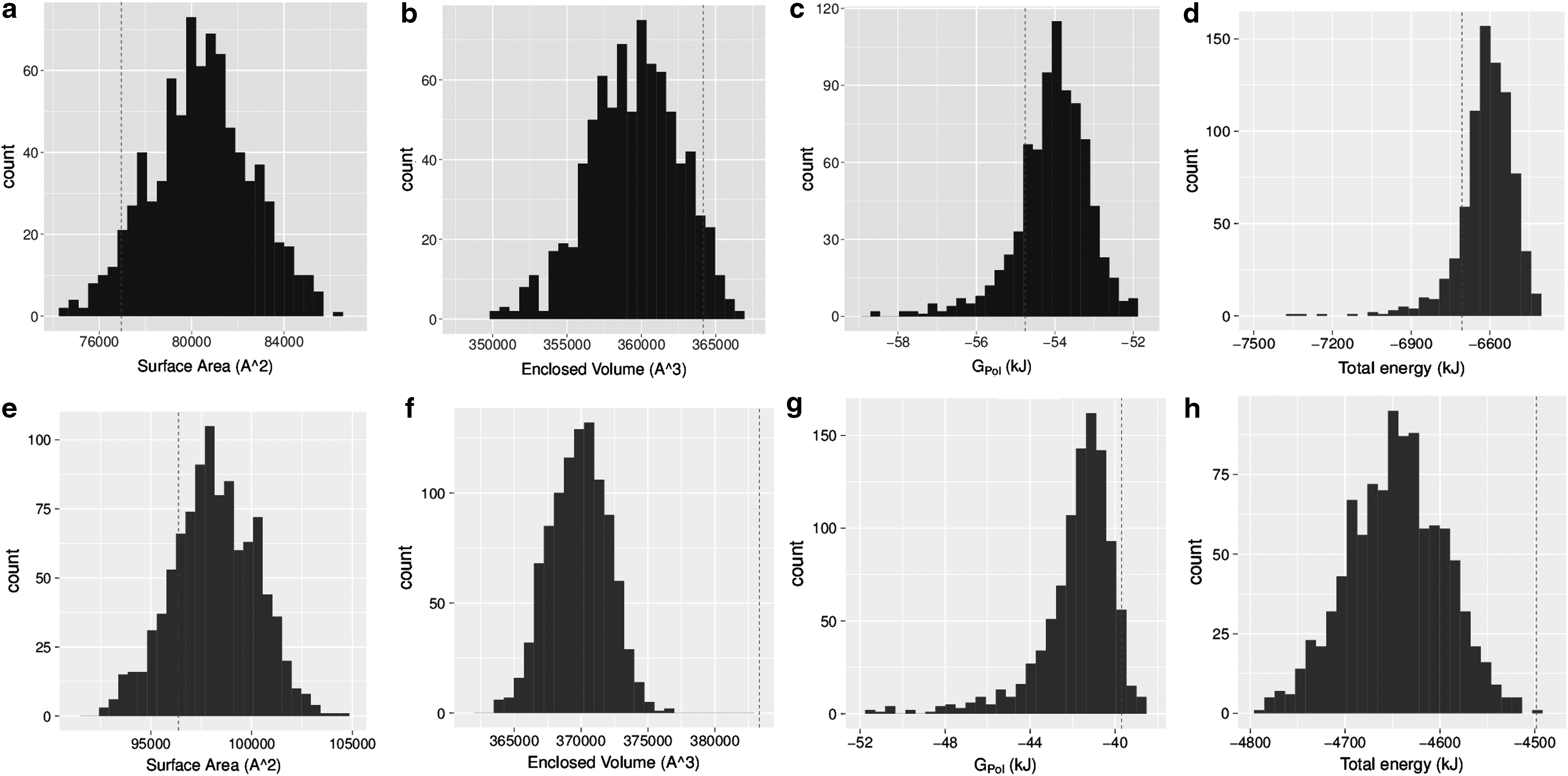
Histogram plots of exposed surface area, enclosed volume, \documentclass{aastex}\usepackage{amsbsy}\usepackage{amsfonts}\usepackage{amssymb}\usepackage{bm}\usepackage{mathrsfs}\usepackage{pifont}\usepackage{stmaryrd}\usepackage{textcomp}\usepackage{portland, xspace}\usepackage{amsmath, amsxtra}\usepackage{upgreek}\pagestyle{empty}\DeclareMathSizes{10}{9}{7}{6}\begin{document} $${G_{pol}}$$ \end{document} , and total energy (GBSA model) for all samples of the pentamer A1-A2-A3-A4-A5 of PDBID:1OHF (a–d) and PDBID:1C8F (e–h). Dotted vertical lines are the quantity computed on the model reported in the PDB. GBSA, generalized born solvent accessible; PDB, protein data bank.

The second observation from these plots is one major motivation for using distributions of quantities instead of single values. In Figure 3, the dotted red line shows the quantity computed on the non-perturbed subassembly. For the pentamer, these values vary wildly from the mean. For the panleukopenia virus (Fig. 3e–h), the energy computed on the original molecule is far worse (more positive) than the majority of the energy values from the sampling protocol. In fact, analyzing the Z-scores for all subassemblies shows that many of them (42%) differ greatly from the sampled mean by more than 1 standard deviation, and many (∼3%) are more than 2 standard deviations away. In addition, subassemblies with a larger number of subunits do not necessarily have higher variance. So, correctly accounting for uncertainty requires distributions of configurations, instead of single molecules.

3.3. Comparing capsomers

Given the distributions of a number of subassemblies for a specific property, we can compare them by using the Wilcoxon signed-rank test and generate a total ordering. This is especially useful in gaining insights (with quantified uncertainty bounds) into the relative binding affinities or stabilities of different capsomers. As the number of potential pathways for the panleukopenia virus are far fewer than those of the N. capensis virus, we will limit the discussion in this section to those of the latter capsid.

Figures 4 and 5 show the distribution of total energy for single subunits and dimer subassemblies of PDBID:1OHF (see Fig. 6 for a surface representation of these complexes), and the top 10 subassemblies of size 3, respectively. According to this test, the most stable subunit is B, the most stable subassembly of size 2 is the B5-C1 dimer, and the most stable subassembly of size 3 is the A1-B1-B5 complex. The least stable complexes are A, the C1-D1 dimer, and the C1-D1-D7 complex (not pictured).

FIG. 4.

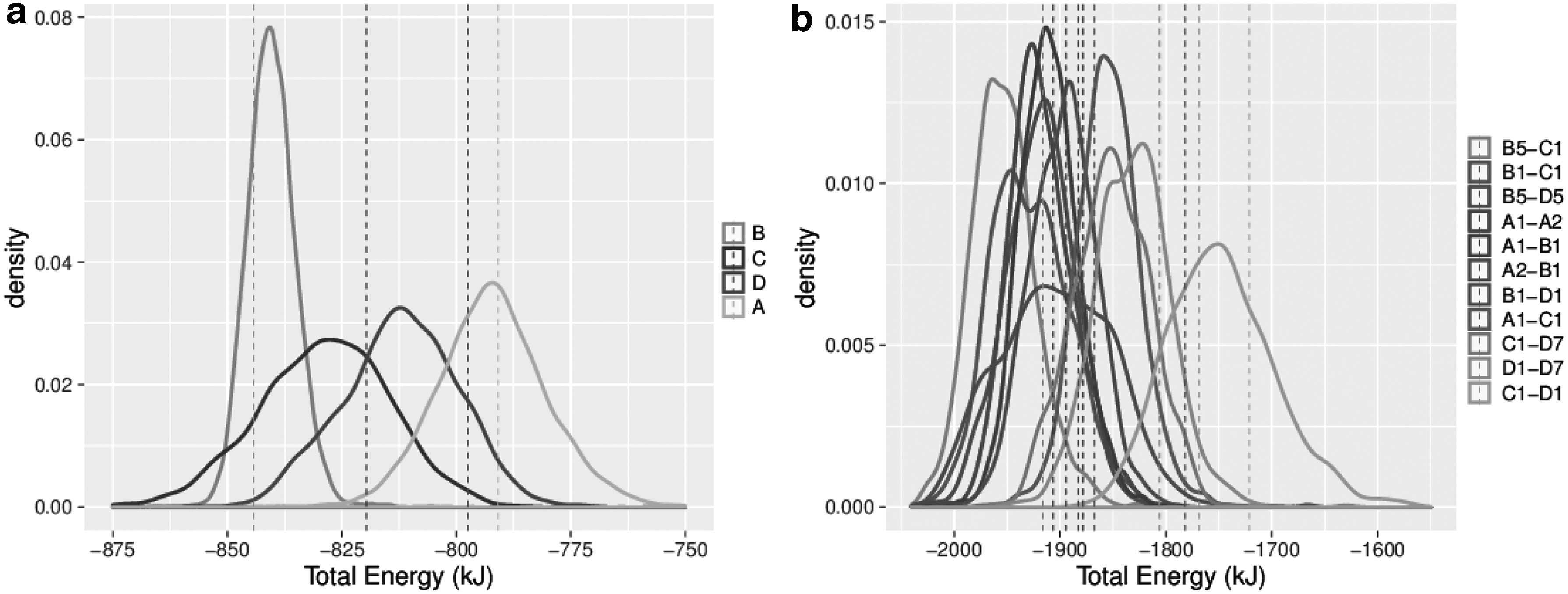
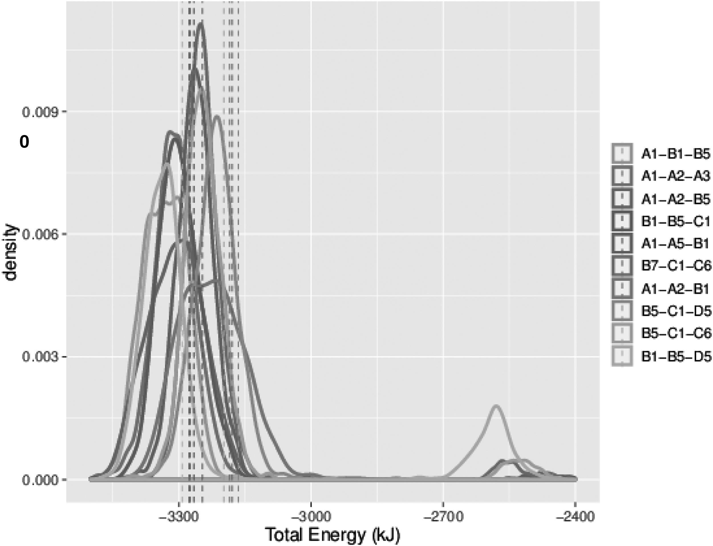
Density plots of distribution of all energy values for all single subunits (a) and subassemblies of size 2 (b) for PDBID:1OHF. Legend is ranked according to the Wilcoxon signed-rank test (top is best), as given in Equation (4).

FIG. 5.

Density plots of distribution of energy values for top 10 subassemblies of size 3 for PDBID:1OHF. Legend is ranked according to the Wilcoxon signed-rank test (top is best), as given in Equation (4).

FIG. 6.

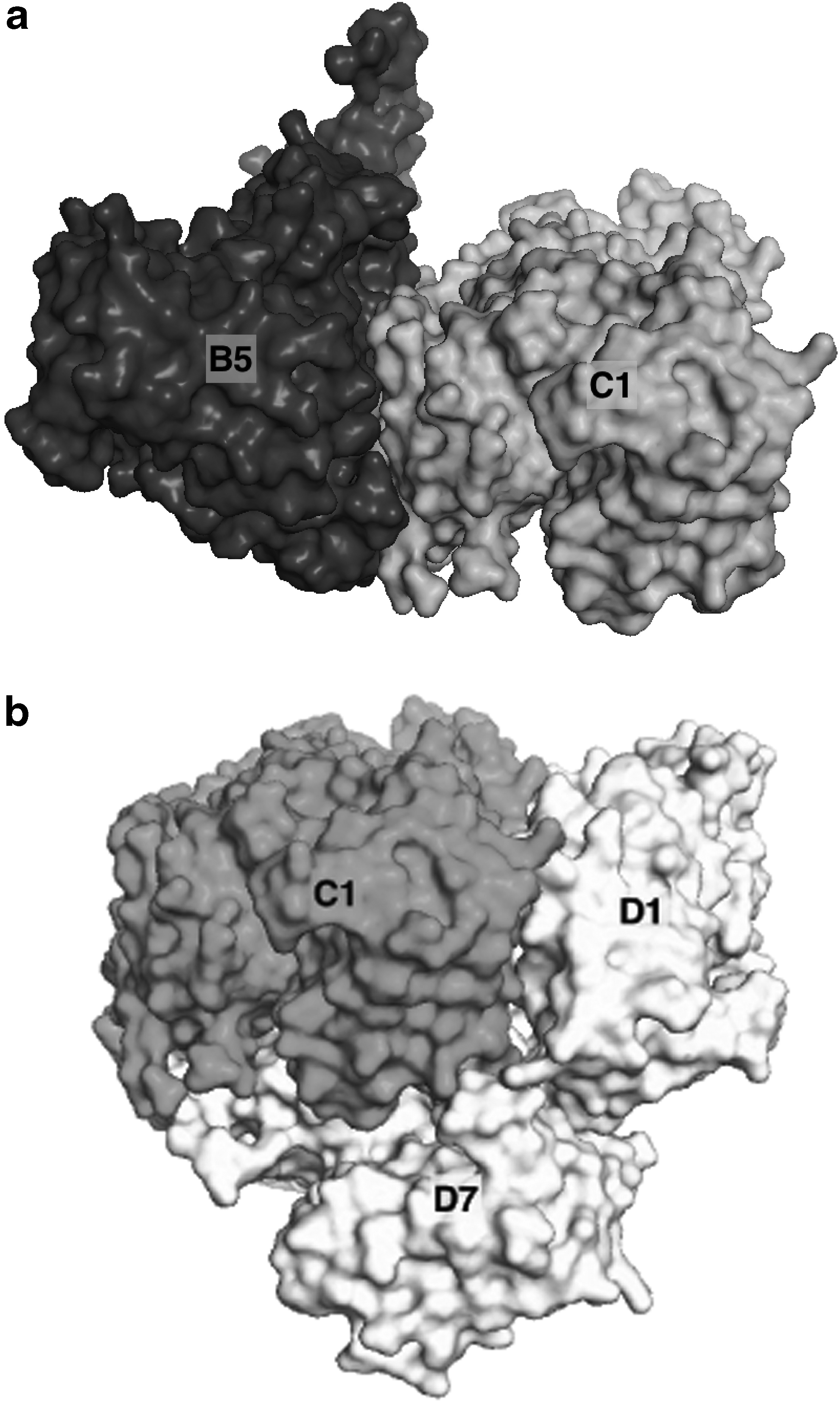
Labeled surface representation of B5-C1 (a), and C1-D1-D7 (b), of PDBID:1OHF. B5-C1 and C1-D1-D7 are the most stable 2- and 3-subunit capsomers.

We also applied the Wilcoxon signed-rank test to rank all possible transitions from any given subassembly, which is a crucial step in predicting/analyzing the assembly pathway. For example, Figure 7 shows the possible state transitions of the N. capensis capsid assembly starting at C1-B5-B1. If only the native configurations were used, one would have reached the conclusion that adding B7 would be the best transition. However, this is an incorrect conclusion since the interface between B7 and B5 has low contact area and is only stable if D7 is also present (see Supplementary Fig. S4 of Clement et al., 2016). That sensitivity is exposed through sampling the local configuration space, which resulted in some configurations with more favorable binding configurations and others that were pulled apart (apparent from the bimodal nature of the distribution). Our method successfully accounted for this uncertainty and, as the Wilcoxon test is robust to these kinds of errors, correctly ranked it lower than other subassemblies.

FIG. 7.

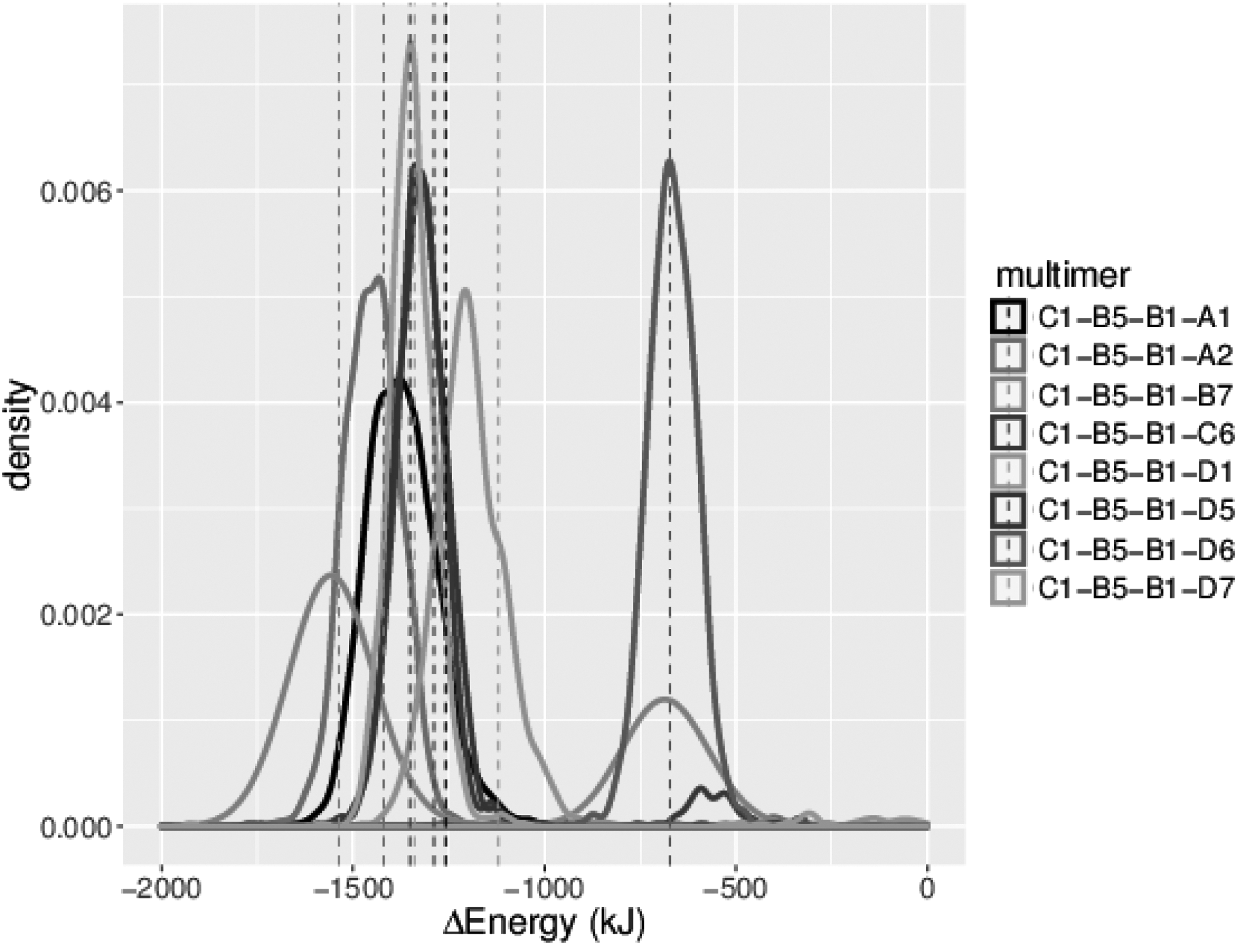
Density plots of distribution of energy values for all possible 4-unit capsomers starting with C1-B5-B1 of PDBID:1OHF. Legend is ranked according to the Wilcoxon signed-rank test (top is best), as given in Equation (4). Dotted vertical lines show the value computed on only the native structure.

3.4. Transitions

Finally, after ranking each transition based off its Wilcoxon score, we construct a complete transition graph showing all possible pathways leading from monomeric subassemblies to the largest subassemblies. Since the entire graph is too large to visually inspect, we present snippets of it here. In addition, limit the discussion in this section to only the N. capensis capsid subassembly. Figure 8 shows transition sub-graphs starting with subunits B5-C1 and C1-D1-D7, respectively. Note that these two were determined to be very stable states according to our analysis presented in the previous subsection. Starting with (C1-B5), the most likely pathway is (C1-B5) \documentclass{aastex}\usepackage{amsbsy}\usepackage{amsfonts}\usepackage{amssymb}\usepackage{bm}\usepackage{mathrsfs}\usepackage{pifont}\usepackage{stmaryrd}\usepackage{textcomp}\usepackage{portland, xspace}\usepackage{amsmath, amsxtra}\usepackage{upgreek}\pagestyle{empty}\DeclareMathSizes{10}{9}{7}{6}\begin{document} $$\to$$ \end{document} B1 \documentclass{aastex}\usepackage{amsbsy}\usepackage{amsfonts}\usepackage{amssymb}\usepackage{bm}\usepackage{mathrsfs}\usepackage{pifont}\usepackage{stmaryrd}\usepackage{textcomp}\usepackage{portland, xspace}\usepackage{amsmath, amsxtra}\usepackage{upgreek}\pagestyle{empty}\DeclareMathSizes{10}{9}{7}{6}\begin{document} $$\to$$ \end{document} A2 \documentclass{aastex}\usepackage{amsbsy}\usepackage{amsfonts}\usepackage{amssymb}\usepackage{bm}\usepackage{mathrsfs}\usepackage{pifont}\usepackage{stmaryrd}\usepackage{textcomp}\usepackage{portland, xspace}\usepackage{amsmath, amsxtra}\usepackage{upgreek}\pagestyle{empty}\DeclareMathSizes{10}{9}{7}{6}\begin{document} $$\to$$ \end{document} A3 \documentclass{aastex}\usepackage{amsbsy}\usepackage{amsfonts}\usepackage{amssymb}\usepackage{bm}\usepackage{mathrsfs}\usepackage{pifont}\usepackage{stmaryrd}\usepackage{textcomp}\usepackage{portland, xspace}\usepackage{amsmath, amsxtra}\usepackage{upgreek}\pagestyle{empty}\DeclareMathSizes{10}{9}{7}{6}\begin{document} $$\to$$ \end{document} A4 (Fig. 8, left). For an assembly process starting with subassembly A1-A2, the most likely pathway is (A1-A2) \documentclass{aastex}\usepackage{amsbsy}\usepackage{amsfonts}\usepackage{amssymb}\usepackage{bm}\usepackage{mathrsfs}\usepackage{pifont}\usepackage{stmaryrd}\usepackage{textcomp}\usepackage{portland, xspace}\usepackage{amsmath, amsxtra}\usepackage{upgreek}\pagestyle{empty}\DeclareMathSizes{10}{9}{7}{6}\begin{document} $$\to$$ \end{document} A3 \documentclass{aastex}\usepackage{amsbsy}\usepackage{amsfonts}\usepackage{amssymb}\usepackage{bm}\usepackage{mathrsfs}\usepackage{pifont}\usepackage{stmaryrd}\usepackage{textcomp}\usepackage{portland, xspace}\usepackage{amsmath, amsxtra}\usepackage{upgreek}\pagestyle{empty}\DeclareMathSizes{10}{9}{7}{6}\begin{document} $$\to$$ \end{document} A4 \documentclass{aastex}\usepackage{amsbsy}\usepackage{amsfonts}\usepackage{amssymb}\usepackage{bm}\usepackage{mathrsfs}\usepackage{pifont}\usepackage{stmaryrd}\usepackage{textcomp}\usepackage{portland, xspace}\usepackage{amsmath, amsxtra}\usepackage{upgreek}\pagestyle{empty}\DeclareMathSizes{10}{9}{7}{6}\begin{document} $$\to$$ \end{document} B5 \documentclass{aastex}\usepackage{amsbsy}\usepackage{amsfonts}\usepackage{amssymb}\usepackage{bm}\usepackage{mathrsfs}\usepackage{pifont}\usepackage{stmaryrd}\usepackage{textcomp}\usepackage{portland, xspace}\usepackage{amsmath, amsxtra}\usepackage{upgreek}\pagestyle{empty}\DeclareMathSizes{10}{9}{7}{6}\begin{document} $$\to$$ \end{document} B1 (Fig. 8, right). This kind of figure can provide a visual method for observing likely state transitions. States that are very likely (such as A2-A3-B1-B5-C1, the last star node on Fig. 8a) have many highly weighted incoming edges (these are “sink” states). States that are not so good can only be reached via poor transitions (such as A1-A5-C1-D1-D7, in Fig. 8b).

FIG. 8.

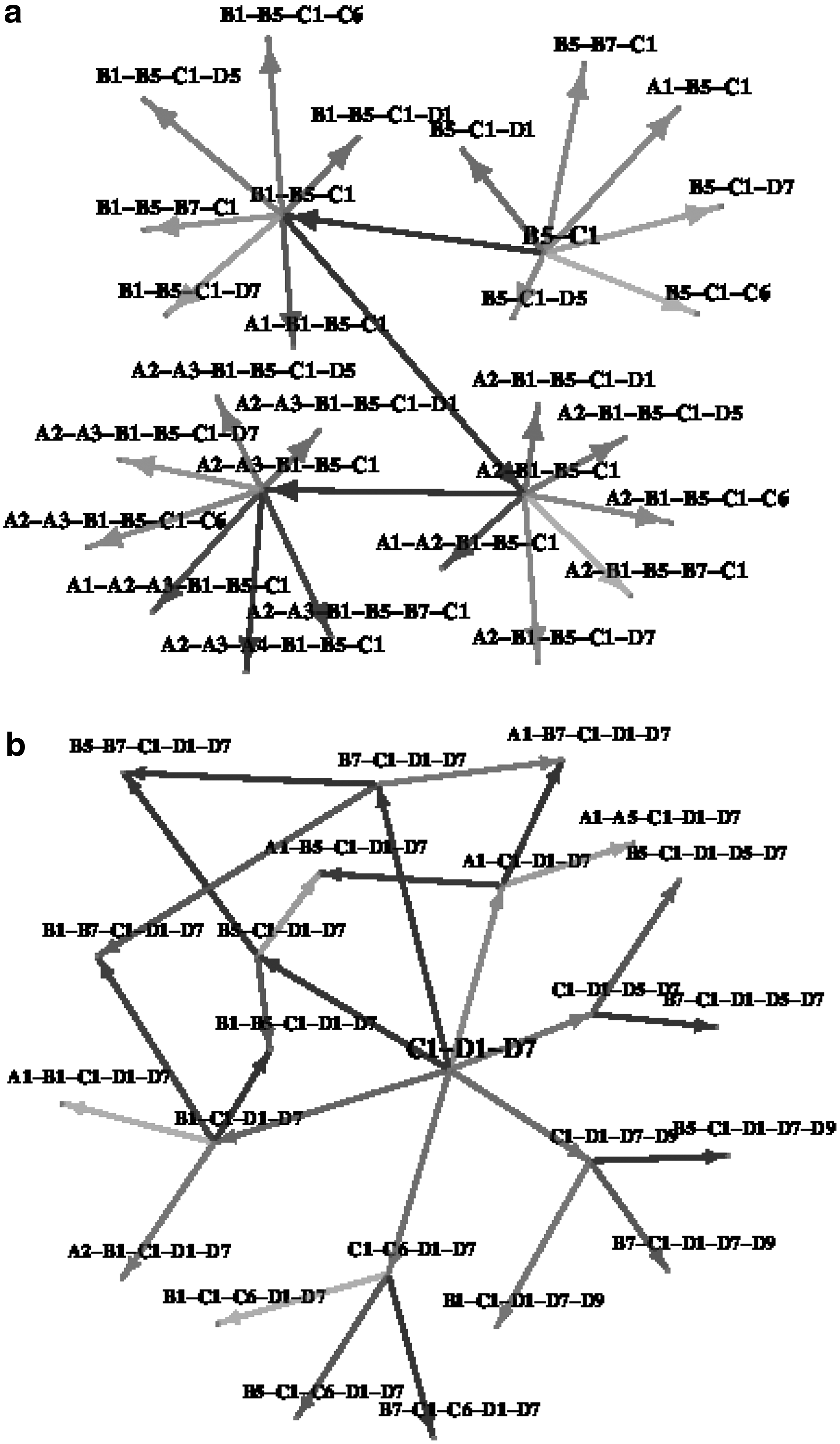
Network graph of possible subassemblies formed when starting from most likely starting points for PDBID:1OHF [(a) B5-C1 dimer and (b) C1-D1-D7 complex]. Color ranges from red (low Wilcoxon score) to gray to blue (high Wilcoxon score). Potential sinks are identified by nodes that have many incoming blue edges, such as A2-B1-B5 on the dimer graph in (a). The B5-C1 complex graph only shows the most likely pathway, and the C1-D1-D7 graph has low-scoring subassemblies removed from the graph for clarity. For more network graphs of individual subunits, please see Supplementary Figures of Clement et al. (2016).

There are several observations that can be made from generating likely pathways. One observation is that A1-A2-A3-A4 is a very stable four-subunit subassembly, whereas A1-A2-A3-A4-B5 is more stable than A1-A2-A3-A4-A5, the pentamer (Fig. 9). This indicates that the pentamer is not fully stabilized until the addition of the B subunit. Such reliance on dimeric interactions may correlate with the size specificity of the virus capsids, since such an interface will not be present in a T = 1 shell. Another insight is that the A-C interface is not at all stable (the C-B or C-D interfaces are much better), and probably does not happen until much later in the assembly process or until other partners on hexameric interfaces provide necessary stabilization.

FIG. 9.

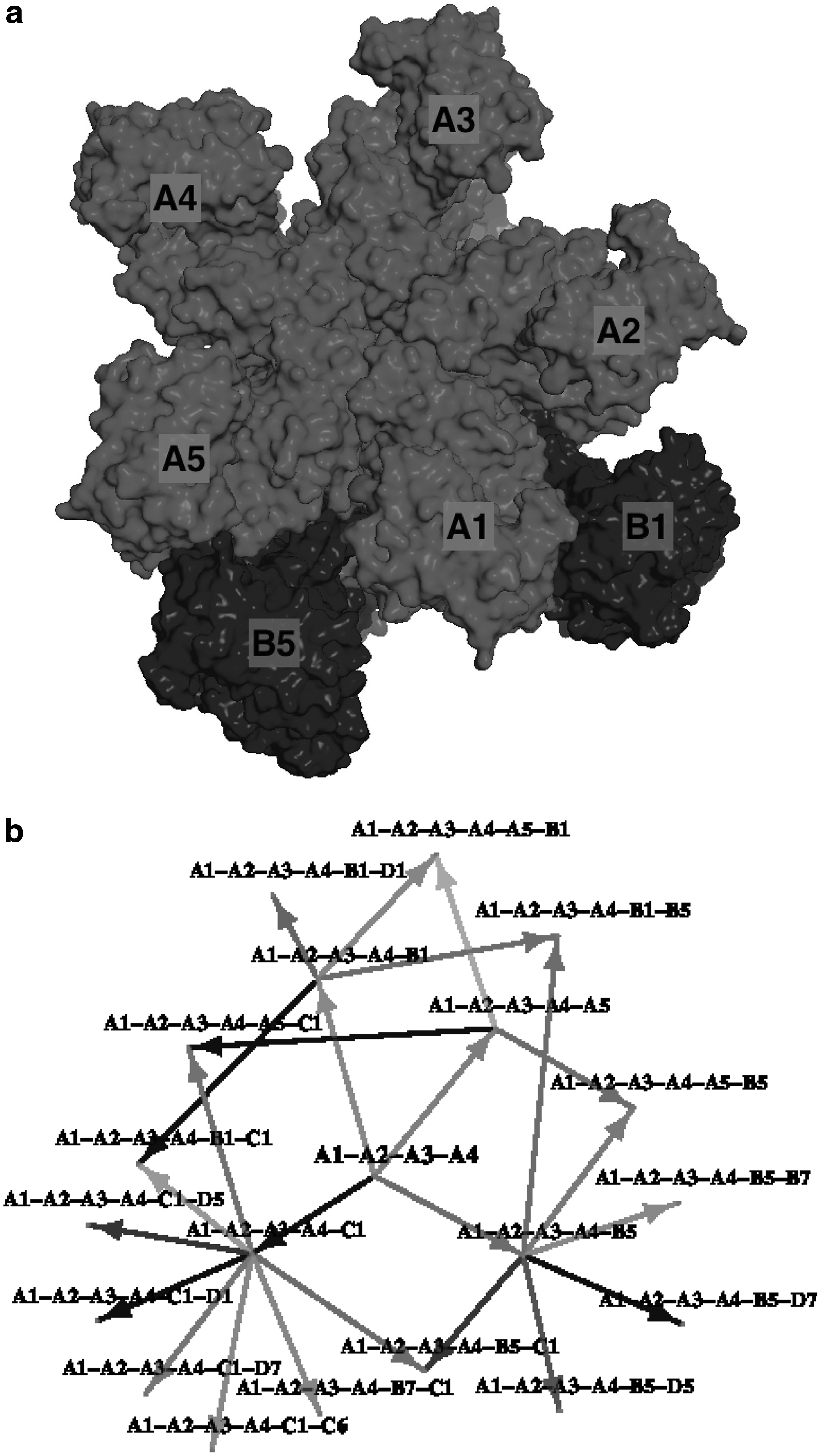
Labeled surface representation of A1-A2-A3-A4-A5-B1-B5 (a), and network graph of possible subassemblies formed when starting from A1-A2-A3-A4 (b) for PDBID:1OHF. Color ranges from red (low Wilcoxon score) to gray to blue (high Wilcoxon score). According to the Wilcoxon test and our results, the final piece of the pentamer does not form until after B1 and B5 have been added.

Finally, we can construct a complete transition graph showing all possible pathways leading from monomeric subassemblies to the largest subassemblies. See Figure 10 for an example where the likely transition pathways based on ΔE are highlighted.

FIG. 10.

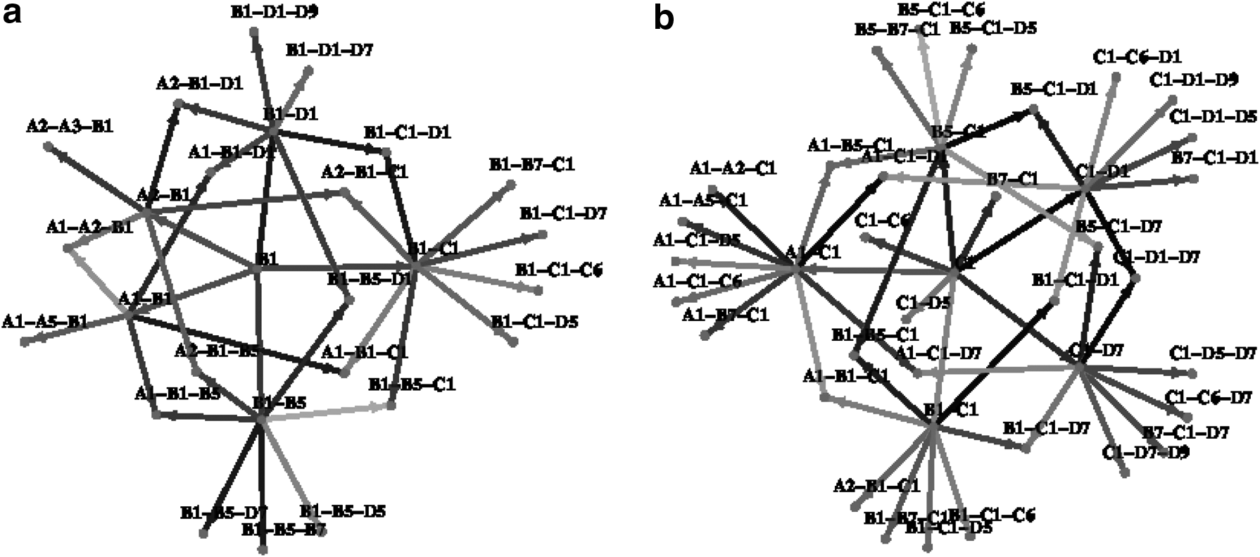
Network graph of possible subassemblies formed up to size 3, when starting from subunit B1 (a) and C1 (b). Color ranges from red (low Wilcoxon score) to gray to blue (high Wilcoxon score).

3.5. Steady-state concentration calculations

Although ΔE is a useful predictor for determining the most likely step in a single-step reaction, it does not take into account one of the major driving forces for chemical reactions: concentrations of the necessary reactants and products. If no reactants are available in a chemical reaction, it cannot take place; likewise, if the concentration of products is too high, the reaction will not proceed. For this reason, we additionally provide a global view of the viral assembly in terms of concentrations of products and reactants.

If the concentration of the reactants, \documentclass{aastex}\usepackage{amsbsy}\usepackage{amsfonts}\usepackage{amssymb}\usepackage{bm}\usepackage{mathrsfs}\usepackage{pifont}\usepackage{stmaryrd}\usepackage{textcomp}\usepackage{portland, xspace}\usepackage{amsmath, amsxtra}\usepackage{upgreek}\pagestyle{empty}\DeclareMathSizes{10}{9}{7}{6}\begin{document} $$[ S ]$$ \end{document} and \documentclass{aastex}\usepackage{amsbsy}\usepackage{amsfonts}\usepackage{amssymb}\usepackage{bm}\usepackage{mathrsfs}\usepackage{pifont}\usepackage{stmaryrd}\usepackage{textcomp}\usepackage{portland, xspace}\usepackage{amsmath, amsxtra}\usepackage{upgreek}\pagestyle{empty}\DeclareMathSizes{10}{9}{7}{6}\begin{document} $$[ {S^{n - 1}} ]$$ \end{document} , and the change in free energy of the subassembly, \documentclass{aastex}\usepackage{amsbsy}\usepackage{amsfonts}\usepackage{amssymb}\usepackage{bm}\usepackage{mathrsfs}\usepackage{pifont}\usepackage{stmaryrd}\usepackage{textcomp}\usepackage{portland, xspace}\usepackage{amsmath, amsxtra}\usepackage{upgreek}\pagestyle{empty}\DeclareMathSizes{10}{9}{7}{6}\begin{document} $$\Delta G ( {S^n} )$$ \end{document} , are known, then it is possible to compute the concentration of the product, \documentclass{aastex}\usepackage{amsbsy}\usepackage{amsfonts}\usepackage{amssymb}\usepackage{bm}\usepackage{mathrsfs}\usepackage{pifont}\usepackage{stmaryrd}\usepackage{textcomp}\usepackage{portland, xspace}\usepackage{amsmath, amsxtra}\usepackage{upgreek}\pagestyle{empty}\DeclareMathSizes{10}{9}{7}{6}\begin{document} $$[ {S^n} ]$$ \end{document} (Zlotnick, 2005): \documentclass{aastex}\usepackage{amsbsy}\usepackage{amsfonts}\usepackage{amssymb}\usepackage{bm}\usepackage{mathrsfs}\usepackage{pifont}\usepackage{stmaryrd}\usepackage{textcomp}\usepackage{portland, xspace}\usepackage{amsmath, amsxtra}\usepackage{upgreek}\pagestyle{empty}\DeclareMathSizes{10}{9}{7}{6}\begin{document} \begin{align*} \left[ { { S^n } } \right] = \left[ { { S^ { n - 1 } } } \right] \left[ S \right] * { \rm { exp } } \left\{ { - { \frac { \Delta G ( { S^n } ) } { RT } } } \right\} \tag { 5 } \end{align*} \end{document}

This can be extended to subassemblies with generic reactants, such as \documentclass{aastex}\usepackage{amsbsy}\usepackage{amsfonts}\usepackage{amssymb}\usepackage{bm}\usepackage{mathrsfs}\usepackage{pifont}\usepackage{stmaryrd}\usepackage{textcomp}\usepackage{portland, xspace}\usepackage{amsmath, amsxtra}\usepackage{upgreek}\pagestyle{empty}\DeclareMathSizes{10}{9}{7}{6}\begin{document} $$B5 - C1$$ \end{document} and \documentclass{aastex}\usepackage{amsbsy}\usepackage{amsfonts}\usepackage{amssymb}\usepackage{bm}\usepackage{mathrsfs}\usepackage{pifont}\usepackage{stmaryrd}\usepackage{textcomp}\usepackage{portland, xspace}\usepackage{amsmath, amsxtra}\usepackage{upgreek}\pagestyle{empty}\DeclareMathSizes{10}{9}{7}{6}\begin{document} $$A1$$ \end{document} , and the product \documentclass{aastex}\usepackage{amsbsy}\usepackage{amsfonts}\usepackage{amssymb}\usepackage{bm}\usepackage{mathrsfs}\usepackage{pifont}\usepackage{stmaryrd}\usepackage{textcomp}\usepackage{portland, xspace}\usepackage{amsmath, amsxtra}\usepackage{upgreek}\pagestyle{empty}\DeclareMathSizes{10}{9}{7}{6}\begin{document} $$A1 - B5 - C1$$ \end{document} , as long as the concentrations of the reactants and \documentclass{aastex}\usepackage{amsbsy}\usepackage{amsfonts}\usepackage{amssymb}\usepackage{bm}\usepackage{mathrsfs}\usepackage{pifont}\usepackage{stmaryrd}\usepackage{textcomp}\usepackage{portland, xspace}\usepackage{amsmath, amsxtra}\usepackage{upgreek}\pagestyle{empty}\DeclareMathSizes{10}{9}{7}{6}\begin{document} $$\Delta G$$ \end{document} of the product formation are known.

It should be noted here that for many chemical reactions, the rate of the reaction is determined by kinetics ( \documentclass{aastex}\usepackage{amsbsy}\usepackage{amsfonts}\usepackage{amssymb}\usepackage{bm}\usepackage{mathrsfs}\usepackage{pifont}\usepackage{stmaryrd}\usepackage{textcomp}\usepackage{portland, xspace}\usepackage{amsmath, amsxtra}\usepackage{upgreek}\pagestyle{empty}\DeclareMathSizes{10}{9}{7}{6}\begin{document} $${k_{{ \rm{assoc}}}}$$ \end{document} and \documentclass{aastex}\usepackage{amsbsy}\usepackage{amsfonts}\usepackage{amssymb}\usepackage{bm}\usepackage{mathrsfs}\usepackage{pifont}\usepackage{stmaryrd}\usepackage{textcomp}\usepackage{portland, xspace}\usepackage{amsmath, amsxtra}\usepackage{upgreek}\pagestyle{empty}\DeclareMathSizes{10}{9}{7}{6}\begin{document} $${k_{{ \rm{dissoc}}}}$$ \end{document} ) and not by thermodynamics \documentclass{aastex}\usepackage{amsbsy}\usepackage{amsfonts}\usepackage{amssymb}\usepackage{bm}\usepackage{mathrsfs}\usepackage{pifont}\usepackage{stmaryrd}\usepackage{textcomp}\usepackage{portland, xspace}\usepackage{amsmath, amsxtra}\usepackage{upgreek}\pagestyle{empty}\DeclareMathSizes{10}{9}{7}{6}\begin{document} $$( \Delta G )$$ \end{document} . However, when the values of \documentclass{aastex}\usepackage{amsbsy}\usepackage{amsfonts}\usepackage{amssymb}\usepackage{bm}\usepackage{mathrsfs}\usepackage{pifont}\usepackage{stmaryrd}\usepackage{textcomp}\usepackage{portland, xspace}\usepackage{amsmath, amsxtra}\usepackage{upgreek}\pagestyle{empty}\DeclareMathSizes{10}{9}{7}{6}\begin{document} $$\Delta G$$ \end{document} are high enough, it can be assumed that the reaction will proceed to completion quickly, and the final ratio of products and reactants will be equal to the equilibrium constant. As the \documentclass{aastex}\usepackage{amsbsy}\usepackage{amsfonts}\usepackage{amssymb}\usepackage{bm}\usepackage{mathrsfs}\usepackage{pifont}\usepackage{stmaryrd}\usepackage{textcomp}\usepackage{portland, xspace}\usepackage{amsmath, amsxtra}\usepackage{upgreek}\pagestyle{empty}\DeclareMathSizes{10}{9}{7}{6}\begin{document} $$\Delta G$$ \end{document} values used in these experiments are very favorable (in the order of 300–3000 kJ/mol), this assumption was made through this section.

Based on Equation (5), it is easy to see that the concentration of a single product is dependent on the concentration of one or more reactants. If concentrations of subassemblies are represented by vertices in a graph, then dependencies can be represented by directional edges in this graph, which have weights proportional to the \documentclass{aastex}\usepackage{amsbsy}\usepackage{amsfonts}\usepackage{amssymb}\usepackage{bm}\usepackage{mathrsfs}\usepackage{pifont}\usepackage{stmaryrd}\usepackage{textcomp}\usepackage{portland, xspace}\usepackage{amsmath, amsxtra}\usepackage{upgreek}\pagestyle{empty}\DeclareMathSizes{10}{9}{7}{6}\begin{document} $$\Delta G$$ \end{document} value for each formation. In this way, we can use a graphical model to describe the assembly process. If we initialize this graphical model with non-zero concentrations for the monomers (A, B, C, and D) and zero concentration for all other nodes and allow concentration to “flow” along edges from one node to another, then the maximum a posteriori probability (MAP) estimate is the steady-state of the graph, where no flow is happening.

3.5.1. Representing capsid assembly as a graph maximum a posteriori probability problem

It is easy to represent the formation of a virus as a Bayesian network consisting of m nodes, where each node represents a possible subassembly, s_k, and the transition probabilities are the rates of formation. A node in the network, \documentclass{aastex}\usepackage{amsbsy}\usepackage{amsfonts}\usepackage{amssymb}\usepackage{bm}\usepackage{mathrsfs}\usepackage{pifont}\usepackage{stmaryrd}\usepackage{textcomp}\usepackage{portland, xspace}\usepackage{amsmath, amsxtra}\usepackage{upgreek}\pagestyle{empty}\DeclareMathSizes{10}{9}{7}{6}\begin{document} $${v_{{s_k}}}$$ \end{document} representing s_k, would have incoming edges from all s_i and s_j, where \documentclass{aastex}\usepackage{amsbsy}\usepackage{amsfonts}\usepackage{amssymb}\usepackage{bm}\usepackage{mathrsfs}\usepackage{pifont}\usepackage{stmaryrd}\usepackage{textcomp}\usepackage{portland, xspace}\usepackage{amsmath, amsxtra}\usepackage{upgreek}\pagestyle{empty}\DeclareMathSizes{10}{9}{7}{6}\begin{document} $$i + j = k$$ \end{document} (e.g., \documentclass{aastex}\usepackage{amsbsy}\usepackage{amsfonts}\usepackage{amssymb}\usepackage{bm}\usepackage{mathrsfs}\usepackage{pifont}\usepackage{stmaryrd}\usepackage{textcomp}\usepackage{portland, xspace}\usepackage{amsmath, amsxtra}\usepackage{upgreek}\pagestyle{empty}\DeclareMathSizes{10}{9}{7}{6}\begin{document} $${s_{k - 1}}$$ \end{document} and s₁, as well as \documentclass{aastex}\usepackage{amsbsy}\usepackage{amsfonts}\usepackage{amssymb}\usepackage{bm}\usepackage{mathrsfs}\usepackage{pifont}\usepackage{stmaryrd}\usepackage{textcomp}\usepackage{portland, xspace}\usepackage{amsmath, amsxtra}\usepackage{upgreek}\pagestyle{empty}\DeclareMathSizes{10}{9}{7}{6}\begin{document} $${s_{k - 2}}$$ \end{document} and s₂, etc.).

However, a limitation of the traditional Bayesian network is that a simple edge weight does not contain all the information necessary to determine forward and backward effects. Instead of a Bayesian network, we can represent the viral assembly process as a Bayesian factor graph, where the factor nodes are states that contain this additional information (Fig. 11). Since we are modeling the creation of a virus from the addition of single subunits, we will enforce an additional constraint that each factor node must have exactly two incoming edges and exactly one outgoing edge.

FIG. 11.

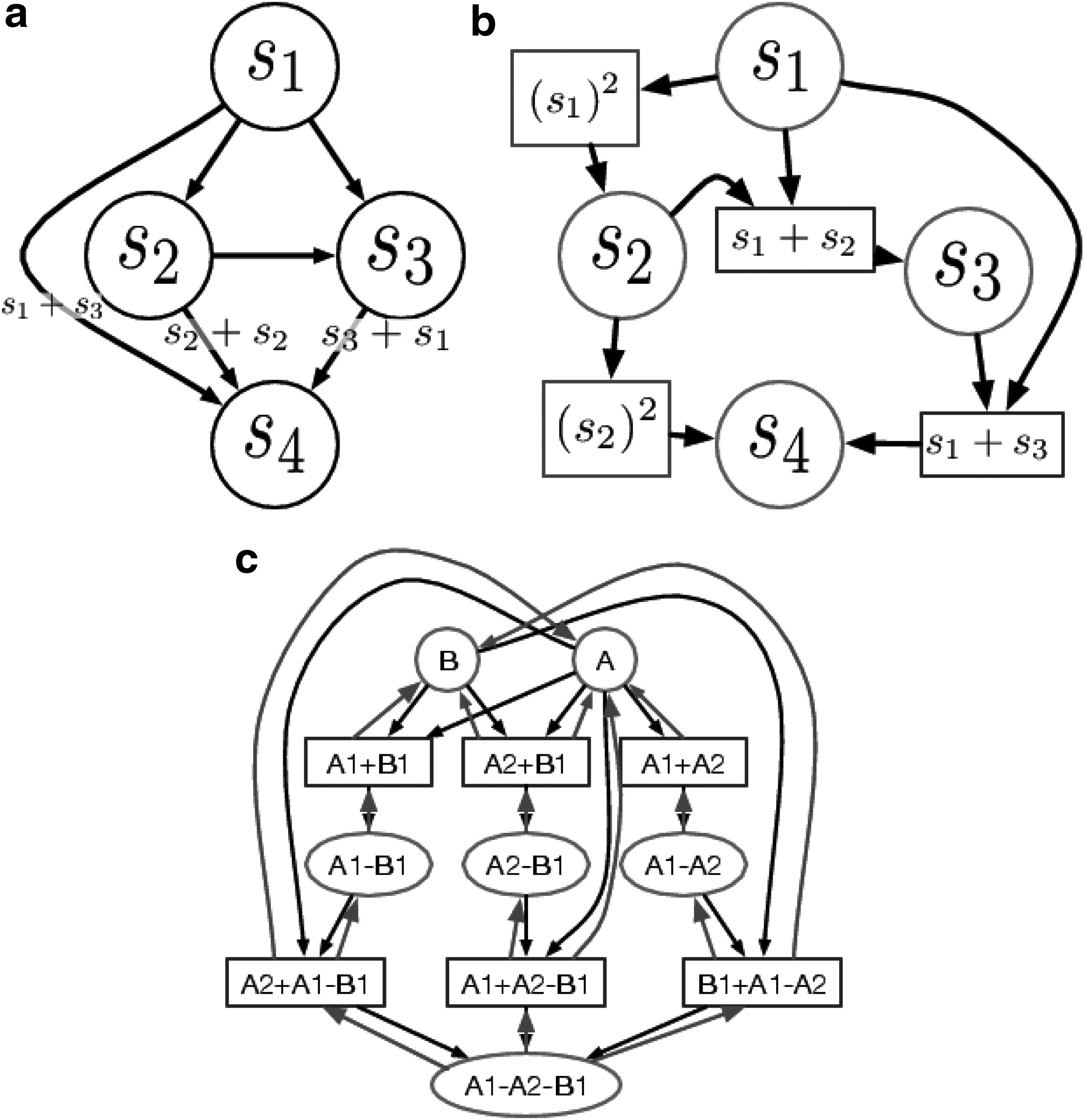
Two different graphical representations of virus formation. (a) A simple directed Bayesian network; (b) the same network represented by a factor graph, where factor nodes are rectangles, representing the combination of a set of smaller nodes. (c) Factor graph for the formation of A1-A2-B1 from all possible units. Variable nodes are red circles, factor nodes are blue rectangles, forward edges are black, and backward edges are green.

3.5.2. Parametrization and solving

Let r be a subunit used to produce more than one product, for example, r and r₁ form p₁, and r and r₂ form p₂. Then, the ratio of the two products can be determined from Equation (5). If we assume that the concentrations of r₁ and r₂ are equal, then: \documentclass{aastex}\usepackage{amsbsy}\usepackage{amsfonts}\usepackage{amssymb}\usepackage{bm}\usepackage{mathrsfs}\usepackage{pifont}\usepackage{stmaryrd}\usepackage{textcomp}\usepackage{portland, xspace}\usepackage{amsmath, amsxtra}\usepackage{upgreek}\pagestyle{empty}\DeclareMathSizes{10}{9}{7}{6}\begin{document} \begin{align*} \left[ {{p_1}} \right] / \left[ {{p_2}} \right] = e ( {p_1} ) / e ( {p_2} ) , \tag{6} \end{align*} \end{document}

For a set of k potential products, \documentclass{aastex}\usepackage{amsbsy}\usepackage{amsfonts}\usepackage{amssymb}\usepackage{bm}\usepackage{mathrsfs}\usepackage{pifont}\usepackage{stmaryrd}\usepackage{textcomp}\usepackage{portland, xspace}\usepackage{amsmath, amsxtra}\usepackage{upgreek}\pagestyle{empty}\DeclareMathSizes{10}{9}{7}{6}\begin{document} $${p_1} \ldots {p_k}$$ \end{document} , the proportional concentration of reactant r that will be used to form product p_i, \documentclass{aastex}\usepackage{amsbsy}\usepackage{amsfonts}\usepackage{amssymb}\usepackage{bm}\usepackage{mathrsfs}\usepackage{pifont}\usepackage{stmaryrd}\usepackage{textcomp}\usepackage{portland, xspace}\usepackage{amsmath, amsxtra}\usepackage{upgreek}\pagestyle{empty}\DeclareMathSizes{10}{9}{7}{6}\begin{document} $$\lambda ( {p_i} )$$ \end{document} , can be written from Equation (6) as: \documentclass{aastex}\usepackage{amsbsy}\usepackage{amsfonts}\usepackage{amssymb}\usepackage{bm}\usepackage{mathrsfs}\usepackage{pifont}\usepackage{stmaryrd}\usepackage{textcomp}\usepackage{portland, xspace}\usepackage{amsmath, amsxtra}\usepackage{upgreek}\pagestyle{empty}\DeclareMathSizes{10}{9}{7}{6}\begin{document} \begin{align*} \lambda ( { p_i } ) = { \frac { e ( { p_i } ) } { \sum \nolimits_ { j = 1 } ^k { e ( { p_j } ) } } } \tag { 7 } \end{align*} \end{document}

Denoting the reverse exponent amount of reactant r as \documentclass{aastex}\usepackage{amsbsy}\usepackage{amsfonts}\usepackage{amssymb}\usepackage{bm}\usepackage{mathrsfs}\usepackage{pifont}\usepackage{stmaryrd}\usepackage{textcomp}\usepackage{portland, xspace}\usepackage{amsmath, amsxtra}\usepackage{upgreek}\pagestyle{empty}\DeclareMathSizes{10}{9}{7}{6}\begin{document} $${e^{ - 1}} ( r )$$ \end{document} and the reverse proportion of a reactant, \documentclass{aastex}\usepackage{amsbsy}\usepackage{amsfonts}\usepackage{amssymb}\usepackage{bm}\usepackage{mathrsfs}\usepackage{pifont}\usepackage{stmaryrd}\usepackage{textcomp}\usepackage{portland, xspace}\usepackage{amsmath, amsxtra}\usepackage{upgreek}\pagestyle{empty}\DeclareMathSizes{10}{9}{7}{6}\begin{document} $${ \lambda ^{ - 1}} ( {r_j} )$$ \end{document} , over a set of potential reactants, \documentclass{aastex}\usepackage{amsbsy}\usepackage{amsfonts}\usepackage{amssymb}\usepackage{bm}\usepackage{mathrsfs}\usepackage{pifont}\usepackage{stmaryrd}\usepackage{textcomp}\usepackage{portland, xspace}\usepackage{amsmath, amsxtra}\usepackage{upgreek}\pagestyle{empty}\DeclareMathSizes{10}{9}{7}{6}\begin{document} $${r_1} \ldots {r_k}$$ \end{document} , we have a similar expression for the reverse reaction: \documentclass{aastex}\usepackage{amsbsy}\usepackage{amsfonts}\usepackage{amssymb}\usepackage{bm}\usepackage{mathrsfs}\usepackage{pifont}\usepackage{stmaryrd}\usepackage{textcomp}\usepackage{portland, xspace}\usepackage{amsmath, amsxtra}\usepackage{upgreek}\pagestyle{empty}\DeclareMathSizes{10}{9}{7}{6}\begin{document} \begin{align*} { \lambda ^ { - 1 } } ( { r_j } ) = { \frac { { e^ { - 1 } } ( { r_i } ) } { \sum \nolimits_ { i = 1 } ^k { { e^ { - 1 } } ( { r_i } ) } } } \tag { 8 } \end{align*} \end{document}

Let \documentclass{aastex}\usepackage{amsbsy}\usepackage{amsfonts}\usepackage{amssymb}\usepackage{bm}\usepackage{mathrsfs}\usepackage{pifont}\usepackage{stmaryrd}\usepackage{textcomp}\usepackage{portland, xspace}\usepackage{amsmath, amsxtra}\usepackage{upgreek}\pagestyle{empty}\DeclareMathSizes{10}{9}{7}{6}\begin{document} $$G = [ E , V , F ]$$ \end{document} be a bipartite graph, G, with edges E and nodes divided into two disjoint groups V (variable nodes, or concentrations of subassemblies) and F (factor “pool” nodes, or hidden nodes where concentrations “pool” before being assembled). Then, the only messages that are passed are from \documentclass{aastex}\usepackage{amsbsy}\usepackage{amsfonts}\usepackage{amssymb}\usepackage{bm}\usepackage{mathrsfs}\usepackage{pifont}\usepackage{stmaryrd}\usepackage{textcomp}\usepackage{portland, xspace}\usepackage{amsmath, amsxtra}\usepackage{upgreek}\pagestyle{empty}\DeclareMathSizes{10}{9}{7}{6}\begin{document} $$v \in V$$ \end{document} to \documentclass{aastex}\usepackage{amsbsy}\usepackage{amsfonts}\usepackage{amssymb}\usepackage{bm}\usepackage{mathrsfs}\usepackage{pifont}\usepackage{stmaryrd}\usepackage{textcomp}\usepackage{portland, xspace}\usepackage{amsmath, amsxtra}\usepackage{upgreek}\pagestyle{empty}\DeclareMathSizes{10}{9}{7}{6}\begin{document} $$a \in F$$ \end{document} and vice versa, and not between two members of the same set. We will also distinguish between forward and backward edges. Forward edges represent the formation of a product by two reactants, and backward edges indicate the break-down of products into reactants. See Figure 11(c) for an example of the formation of A1-A2-B1 from all possible reactants.

The traditional method for solving the steady state of a Bayesian factor graph is through a technique called belief propagation or message passing, where each node in the graph will “propagate” its “belief” about the current state of the network to its neighbors (Yedidia et al., 2003). We adopted the traditional sum-product belief propagation method to our problem (Kschischang et al., 2001). Please see Clement et al. (2016) for further details.

To analyze the steady-state (MAP) estimate of the two viral capsids considered in this study, we set the initial concentration of all monomers (A, B, C, and D) to typical micromolar ranges (100 nM). Weights for the factor graph were set to a single \documentclass{aastex}\usepackage{amsbsy}\usepackage{amsfonts}\usepackage{amssymb}\usepackage{bm}\usepackage{mathrsfs}\usepackage{pifont}\usepackage{stmaryrd}\usepackage{textcomp}\usepackage{portland, xspace}\usepackage{amsmath, amsxtra}\usepackage{upgreek}\pagestyle{empty}\DeclareMathSizes{10}{9}{7}{6}\begin{document} $$\Delta E$$ \end{document} value, and the message-passing algorithm was run until concentration change was below 1e-2 nM, summed over all concentration nodes.

3.5.3. Steady-state concentrations

Figure 12 shows the distribution over successive steps of the message-passing algorithm for both capsids, which attempts to model the self-assembly of the capsid. For the most part, the assemblies with higher concentrations at the steady state (final step of the algorithm) are those with more subunits (e.g., the concentration of the hexamer B5-B7-C1-C6-D5-D7 for PDBID:1OHF was 26 nM, several orders of magnitude higher than the other subassemblies; the concentrations of most dimer and trimer subassemblies for PDBID:1C8F have a quick spike, then rapidly decrease; etc.). This observation would suggest that the subassembly formation largely proceeded toward completion of products, and that the limiting factor was concentration of the products, as was expected. However, not all of the results were consistent with this intuition. Notably, the dimeric interface A1-A6 from the panleukopenia virus was extremely strong (having more than one binding footprint), and it had the highest final concentration (26 nM) (the second highest final concentration was 23 nM for A1-A2-A5-A6-A7-A9, which still did not contain the pentamer).

FIG. 12.

Change in concentration over time for several subassemblies of the N. capensis (a) and panleukopenia (b) virus capsids, when average \documentclass{aastex}\usepackage{amsbsy}\usepackage{amsfonts}\usepackage{amssymb}\usepackage{bm}\usepackage{mathrsfs}\usepackage{pifont}\usepackage{stmaryrd}\usepackage{textcomp}\usepackage{portland, xspace}\usepackage{amsmath, amsxtra}\usepackage{upgreek}\pagestyle{empty}\DeclareMathSizes{10}{9}{7}{6}\begin{document} $$\Delta E$$ \end{document} energy values are considered. The legend in each plot is sorted according to concentration at the final step in the plot. The x-axis has been trimmed to emphasize initial concentration changes, as the steady-state concentrations were reached after 1300 steps of the algorithm.

An important point to note is that this graph would be somewhat different if subassemblies of size greater than 6 were also included, as the intermediate products would be quickly consumed. From Figure 12, this phenomenon can already be observed on both viral capsids; for example, the intermediate product A1-C1 of PDBID:1OHF has an initial high concentration, but then quickly drops off as it is used for later products, such as A1-B1-C1-D1. This also explains why the concentration of monomer C decays so slowly, as there are fewer beneficial reactions involving C (see, for e.g., Fig. 5, where the products involving C are not highly ranked). This might suggest that the configuration of C with the rest of the capsid is meant as a stabilizing subassembly, and is not used until much later in the assembly process.

Finally, we can also plot the distribution of all possible steady-state concentrations, shown in Figure 13. For this plot, initial values of \documentclass{aastex}\usepackage{amsbsy}\usepackage{amsfonts}\usepackage{amssymb}\usepackage{bm}\usepackage{mathrsfs}\usepackage{pifont}\usepackage{stmaryrd}\usepackage{textcomp}\usepackage{portland, xspace}\usepackage{amsmath, amsxtra}\usepackage{upgreek}\pagestyle{empty}\DeclareMathSizes{10}{9}{7}{6}\begin{document} $$\Delta G$$ \end{document} were sampled from the distribution of possible values for each subassembly, and then the steady-state assembly algorithm was run as usual. The final (steady-state) values for each subassembly were recorded, and the distributions of final concentrations were plotted as box-and-whisker plots. In the figure, the red dot shows the steady-state value computed when using just the value of \documentclass{aastex}\usepackage{amsbsy}\usepackage{amsfonts}\usepackage{amssymb}\usepackage{bm}\usepackage{mathrsfs}\usepackage{pifont}\usepackage{stmaryrd}\usepackage{textcomp}\usepackage{portland, xspace}\usepackage{amsmath, amsxtra}\usepackage{upgreek}\pagestyle{empty}\DeclareMathSizes{10}{9}{7}{6}\begin{document} $$\Delta G$$ \end{document} computed on the initial structure from the protein data bank (PDB). For the panleukopenia virus, the results obtained from the original protein are usually within the first and third quartile of the distribution; however, the N. capensis virus (Fig. 13a) shows several subassemblies (A1-B1 and D1-D7-D9) where the value computed with the original statistic is greatly misleading.

FIG. 13.

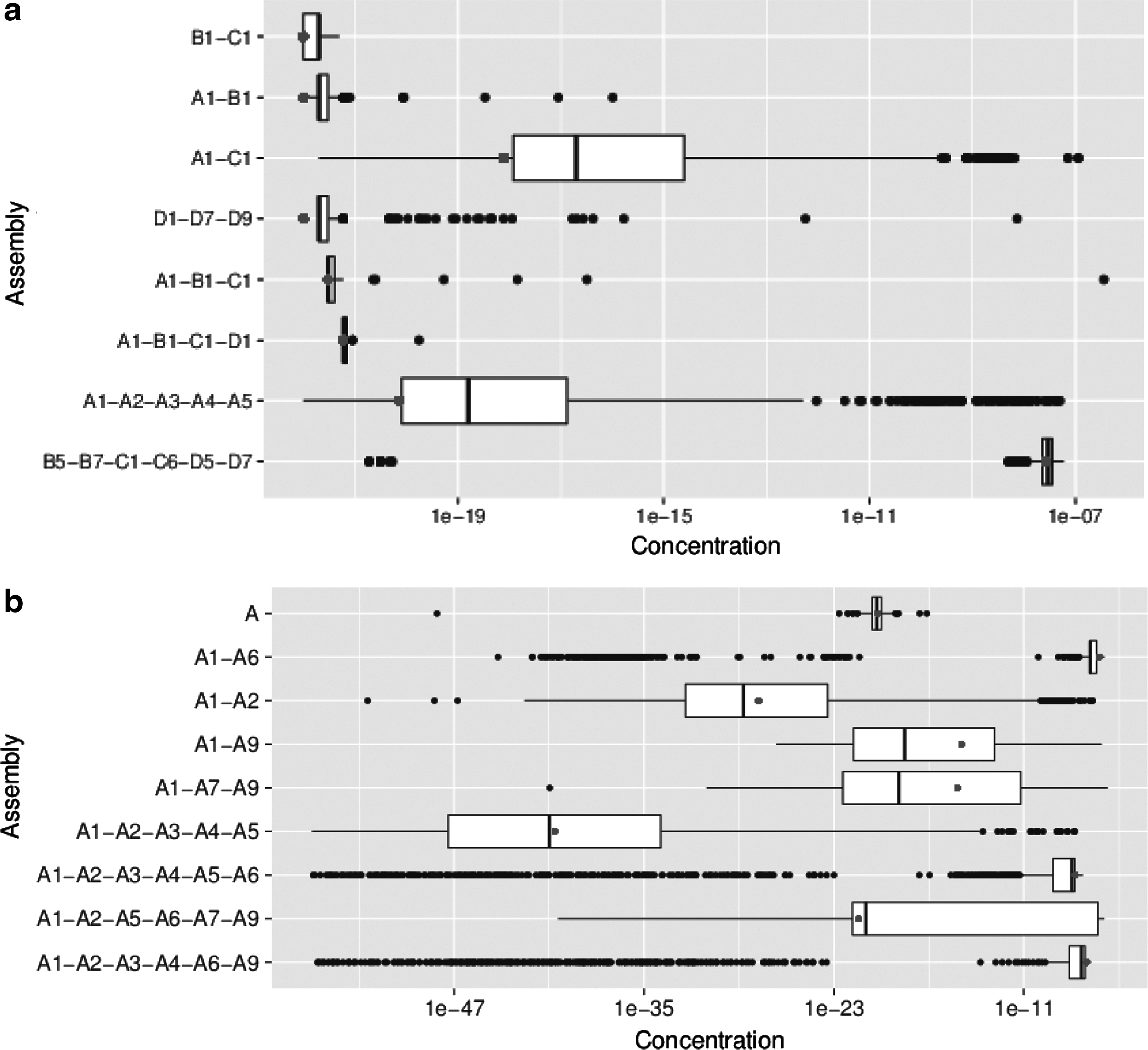
Distribution of concentrations over different input \documentclass{aastex}\usepackage{amsbsy}\usepackage{amsfonts}\usepackage{amssymb}\usepackage{bm}\usepackage{mathrsfs}\usepackage{pifont}\usepackage{stmaryrd}\usepackage{textcomp}\usepackage{portland, xspace}\usepackage{amsmath, amsxtra}\usepackage{upgreek}\pagestyle{empty}\DeclareMathSizes{10}{9}{7}{6}\begin{document} $$\Delta G$$ \end{document} values, for various subassemblies of the N. capensis (a) and panleukopenia (b) virus capsids. x-Axis is log-scale to emphasize differences. Red point is value computed when using just the original PDB.

This kind of plot illuminates several things: first, that the distributions of final concentrations can differ greatly across subassemblies. If only a single input model is used and only a single statistic is reported, the entire landscape of possible values is overlooked. Second, the value computed on the original PDB does not represent the true average across all samples, further supporting the need to analyze capsid assembly through distributions of values.

4. Conclusions

Most of the existing research in assembly pathway prediction/analysis of virus capsids has relied on the final configuration of the capsid to determine the configuration of the intermediate states. This assumption is overly simplified since the capsid proteins may undergo conformational changes, binding interfaces adjustments to allow binding with another subassembly, etc., throughout the assembly process until stabilization. To better capture this phenomenon, we have developed a statistical-ensemble-based approach that sufficiently samples the configurational space of each monomer and the relative local orientation between monomers to capture the uncertainties in their binding. Instead of modeling each subassembly as a static configuration, we model them as distributions of possible configurations. This allows us to compute distributions of free energy over many subassembly samples, and to use distributions of binding free energy on a possible assembly edge instead of a single quantity so that statistical guarantees of accuracy can additionally be derived for each of the resulting assemblies.

Unlike traditional approaches where pentamers, hexamers, or trimers are used as fundamental building blocks in the assembly pathway analysis, we use individual monomers as our starting constituents, and consider all possible unique subassemblies (modulo symmetry), of sizes up to 6. The primary aim is to quantitatively understand the formation of the larger building blocks (i.e., trimers, pentamers, and hexamers).

We additionally adapted the Wilcoxon measure to provide a way to compare the distributions and determine the most likely subassemblies that can be generated in any step. Using this score as weights on an assembly graph revealed that there are some low-energy subassemblies that are unlikely to be formed because there are poor transitions along the path that form the said subassembly. We proposed an assembly prediction algorithm that utilizes both binding free energy and equilibrium concentrations, and we applied it to two different capsid assembly problems. The algorithm uses a Bayesian factor graph where the final concentrations of the subassemblies are posed as a graphical maximum a posteriori problem. Transition probabilities were set up based on the equilibrium constant computed from the binding free energy, and both forward (association) and backward (dissociation) reactions were allowed. The result showed expected patterns, for example, dimers A1-B1, A1-A2, etc., being produced at a fast rate initially and then being consumed as other subassemblies become available, forming the larger subassemblies A1-B1-C1 (trimer), A1-A2-A3-A4-A5 (pentamer), etc. As the concentrations reach their steady state, larger particles had higher final concentrations, as was expected. The algorithm also highlighted several differences between the two viruses considered, some of which were contrary to intuition.

In summary, we contend that the use of ensemble distributions of molecules, instead of single conformations, allows one to make statistical inferences about the stability of molecular subassemblies. We have shown that a full distribution of possible subassemblies is not obtainable if one was to use assembly combinations only from the original PDB conformation. This could often lead to erroneous conclusions. Use of a statistically rigorous procedure, such as the one advocated in this article, yields inferences on capsid assembly that can be made with statistical confidence.

Footnotes

Acknowledgments

This research was supported in part by NIH-R01GM117594, NIH-R41GM116300 and a grant from SETON-Dell Medical 201602388.

Author Disclosure Statement

No competing financial interests exist.

References

Azuma

1967. Weighted sums of certain dependent random variables. Tokuku Math. J. 19, 357–367.

Bajaj

, Bhowmick

, Chattopadhyay

, et al. 2014. On low discrepancy samplings in product spaces of motion groups. arXiv.org e-Print archive. Available at: http://arxiv.org/abs/1411.7753. Last accessed in Nov. 2014.

Bajaj

, Chowdhury

R.A.

, and Rasheed

2011. A dynamic data structure for flexible molecular maintenance and informatics. Bioinformatics, 27, 55–62.

Bajaj

, and Zhao

2010. Fast molecular solvation energetics and forces computation. SIAM J. Sci. Comput. 31, 4524–4552.

Berger

, and Shor

P.W.

1994. On the Mathematics of Virus Shell Assembly. MIT Center for Advanced Education Services. Boston, MA.

Berger

, Shor

P.W.

, Tucker-Kellogg

, et al. 1994. Local rule-based theory of virus shell assembly. Proc. Natl Acad. Sci. U. S. A., 91, 7732–7736.

Bona

, Sitharam

, and Vince

2011. Enumeration of viral capsid assembly pathways: Tree orbits under permutation group action. Bull. Math. Biol., 73, 726–753.

Burns

, Mukherjee

, Keef

, et al. 2009. Altering the energy landscape of virus self-assembly to generate kinetically trapped nanoparticles. Biomacromolecules. 11, 439–442.

Carrillo-Tripp

, Brooks

C.L.

, and Reddy

V.S.

2008. A novel method to map and compare protein-protein interactions in spherical viral capsids. Proteins, 73, 644–655.

10.

Case

D.A.

, Cheatham

T.E.

, Darden

, et al. 2005. The amber biomolecular simulation programs. J. Comput. Chem., 26, 1668–1688.

11.

Caspar

D.L.

, and Klug

1962. Physical principles in the construction of regular viruses. Cold Spring Harb. Symp. Quant. Biol. 27, 1–24.

12.

Cha

, Zhang

, Tithi

J.J.

, et al. (2015). Accelerated molecular mechanical and solvation energetics on multicore CPUs and manycore GPUs. In Proceedings of the 6th ACM Conference on Bioinformatics, Computational Biology and Health Informatics, pp. 222–231. ACM. Washington, DC.

13.

Cheng

, Samia

, Meyers

, et al. 2008. Highly efficient drug delivery with gold nanoparticle vectors for in vivo photodynamic therapy of cancer. J. Am. Chem. Soc., 130, 10643–10647.

14.

Clement

N.L.

, Rasheed

, and Bajaj

C.L.

2016. Uncertainty quantified computational analysis of the energetics of virus capsid assembly. arXiv.org e-Print archive. Available at: https://arxiv.org/abs/1610.00638. Last accessed in Oct. 2016.

15.

Damodaran

, Reddy

V.S.

, Johnson

J.E.

, et al. 2002. A general method to quantify quasi-equivalence in icosahedral viruses. J. Mol. Biol., 324, 723–737.

16.

Elrad

O.M.

, and Hagan

M.F.

2008. Mechanisms of size control and polymorphism in viral capsid assembly. Nano Lett. 8, 3850–3857.

17.

Emekli

, Schneidman-Duhovny

, Wolfson

H. J.

, et al. 2008. HingeProt: Automated prediction of hinges in protein structures. Proteins, 70, 1219–1227.

18.

Goldberg

1937. A class of multi-symmetric polyhedra. Tohoku Math. J. 43, 104–108.

19.

Hagan

M.F.

2014. Modeling viral capsid assembly. Adv. Chem. Phys., 155, 1–68.

20.

Hagan

M.F.

, and Chandler

2006. Dynamic pathways for viral capsid assembly. Biophys. J., 91, 42–54.

21.

Helgstrand

, Munshi

, Johnson

J.E.

, et al. 2004. The refined structure of Nudaurelia capensis

virus reveals control elements for a

capsid maturation. Virology, 318, 192–203.

22.

Hoeffding

1963. Probability inequalities for sums of bounded random variables. J. Am. Stat. Assoc., 58, 13–30.

23.

Hoogland

, James

, and Kleiss

1998. Quasi-monte carlo, discrepancies and error estimates, 266–276. In Niederreiter

, Hellekalek

, Larcher

, and Zinterhof

, eds, Monte Carlo and Quasi-Monte Carlo Methods 1996. Springer New York, New York, NY.

24.

Janner

2006. Towards a classification of icosahedral viruses in terms of indexed polyhedra. Acta Crystallogr. A62, 319–330.

25.

Keef

, and Twarock

2009. Affine extensions of the icosahedral group with applications to the three-dimensional organisation of simple viruses. J. Math. Biol., 3, 287–313.

26.

Kschischang

F.R.

, Frey

B.J.

, and Loeliger

H.-A.

2001. Factor graphs and the sum-product algorithm. IEEE Trans. Inf. Theory, 47, 498–519.

27.

Lai

, Tsai

K.L.

, Sawaya

, et al. 2013. Structure and flexibility of nanoscale protein cages designed by symmetric self-assembly. J. Am. Chem. Soc., 135, 7738–7743.

28.

Lei

, Yang

, Zheng

, et al. 2014. Quantifying the influence of conformational uncertainty in biomolecular solvation. arXiv.org e-Print archive. Available at: http://arxiv.org/abs/1408.5629. Last accessed in Aug. 2015.

29.

Mannige

R.V.

, and Brooks

C.L.

III . 2008. Tilable nature of virus capsids and the role of topological constraints in natural capsid design. Phys. Rev. E Stat. Nonlin. Soft Matter Phys., 77, 051902–051909.

30.

Mannige

R.V.

, and Brooks

C.L.

III , 2010. Periodic table of virus capsids: Implications for natural selection and design. PLoS One. 5, 7.

31.

McDiarmid

1989. On the method of bounded differences. Surv. Combinatorics, 141, 148–188.

32.

Niederreiter

1990. Quasi-Monte Carlo methods. Encyclopedia Quant. Finance, 24, 55–61.

33.

Niederreiter

1992. Random Number Generation and Quasi-Monte Carlo Methods. Society for Industrial and Applied Mathematics, Philadelphia, PA.

34.

Pawley

1961. Plane groups on polyhedra. Acta Crystallogr. 15, 49–53.

35.

Rapaport

D.C.

2004. Self-assembly of polyhedral shells: A molecular dynamics study. Phys. Rev. E., 70, 1–13.

36.

Rapaport

D.C.

2010. Modeling capsid self-assembly: Design and analysis. Phys. Biol. 7, 045001.

37.

Rapaport

D.C.

, Johnson

J.E.

, and Skolnick

1999. Supramolecular self-assembly: Molecular dynamics modeling of polyhedral shell formation. Comput. Phys. Commun., 121, 231–235.

38.

Rasheed

, and Bajaj

2015. Highly symmetric and congruently tiled meshes for shells and domes. Procedia Eng. 124, 213–225.

39.

Rasheed

, Clement

, Bhowmick

, et al. 2015. Quantifying and visualizing uncertainties in molecular models. arXiv.org e-Print archive. Available at: http://arxiv.org/abs/1508.03882v2. Last accessed in May 2016. (Also appears in enhanced form: IEEE/ACM Trans. on Comp. Bio and Bioinformatics, vol. 14, 2017.)

40.

Schwartz

, Shor

, Prevelige

, et al. 1998. Local rules simulation of the kinetics of virus capsid self-assembly. Biophys. J., 75:2626–2636.

41.

Simpson

A.A.

, Chandrasekar

, Hébert

, et al. 2000. Host range and variability of calcium binding by surface loops in the capsids of canine and feline parvoviruses. J Mol Biol. 300:597–610.

42.

Sitharam

, Ozkan

, Pence

, et al. 2004. EASAL: Efficient atlasing, analysis and search of molecular assembly landscapes. arXiv.org e-Print archive. Available at: http://arxiv.org/abs/1203.3811. Last accessed in March 2012.

43.

Smith

M.T.

, Hawes

A.K.

, and Bundy

B.C.

2013. Reengineering viruses and virus-like particles through chemical functionalization strategies. Curr. Opin. Biotechnol., 24, 620–626.

44.

Wilcoxon

1945. Individual comparisons by ranking methods. Biometr. Bull., 1, 80–83.

45.

Xie

, Smith

G. R.

, Feng

, et al. 2012. Surveying capsid assembly pathways through simulation-based data fitting. Biophys. J., 103, 1545–1554.

46.

Yedidia

J.S.

, Freeman

W.T.

, and Weiss

2003. Understanding belief propagation and its generalizations, 236–239. In Exploring Artificial Intelligence in the New Millennium, Vol. 8. Morgan Kaufmann Publishers, San Francisco, CA.

47.

Zlotnick

1994. To build a virus capsid: An equilibrium model of the self assembly of polyhedral protein complexes. J. Mol. Biol., 241, 59–67.

48.

Zlotnick

2005. Theoretical aspects of virus capsid assembly. J. Mol. Recognit., 18, 479–490.

49.

Zlotnick

2006. Distinguishing reversible from irreversible virus capsid assembly. J. Mol. Biol., 366, 14–18.

50.

Zlotnick

, and Mukhopadhyay

2011. Virus assembly, allostery and antivirals. Trends Microbiol. 19, 14–23.

51.

Zochowska

, Paca

, Schoehn

, et al. 2009. Adenovirus dodecahedron, as a drug delivery vector. PLoS One, 4, 1–12.