Machine learning methods for learning network structure are applied to quantitative proteomics experiments and reverse-engineer intracellular signal transduction networks. They provide insight into the rewiring of signaling within the context of a disease or a phenotype. To learn the causal patterns of influence between proteins in the network, the methods require experiments that include targeted interventions that fix the activity of specific proteins. However, the interventions are costly and add experimental complexity.
We describe an active learning strategy for selecting optimal interventions. Our approach takes as inputs pathway databases and historic data sets, expresses them in form of prior probability distributions on network structures, and selects interventions that maximize their expected contribution to structure learning. Evaluations on simulated and real data show that the strategy reduces the detection error of validated edges as compared with an unguided choice of interventions and avoids redundant interventions, thereby increasing the effectiveness of the experiment.
1. Introduction
Signaling networks describe chains of protein interactions that determine how cells process signals from their environment. The deregulation of signaling networks occurs under many conditions, for example, in diseases such as cancer (Pawson and Warner, 2007), gene knockouts, or introduction of a drug. The patterns of such deregulation can be inferred from quantitative proteomic experiments conducted under the conditions of interest, using causal inference and Bayesian networks (Friedman, 2004; Sachs et al., 2005).
In these investigations, signaling is induced with a stimulus perturbation, and a measurement technology acquires information on the activity of signaling proteins (Terfve et al., 2012). Bulk experiments quantify aggregate signaling activity across a sample. In contrast, single-cell technologies provide cell-level resolution of signaling activity. For example, in flow cytometry, cells are chemically fixed, and intracellular signaling proteins are tagged with fluorescently labeled antibodies. The cytometer then records the antibodies' fluorescence in individual cells, each reflecting the relative abundance of signaling proteins in different states of enzymatic activity (Perez and Nolan 2002). Similarly, in mass cytometry (CyTOF) experiments, intracellular signaling proteins are tagged with heavy-metal isotopes, and the mass spectrometer records the mass-to-charge ratio of the charged isotope tags (Bandura et al., 2009).
Causal Bayesian networks represent signaling proteins as nodes and regulatory relationships as directed edges. It interprets a network as a topological map of the underlying signaling network. By comparing the structure inferred under a condition with canonical pathways in sources such as KEGG and Reactome, we can learn the patterns of network deregulation. Data repositories, such as Cytobank (Chen and Kotecha, 2014), provide historic data, which can be incorporated in the analysis and interpretation of experimental results (Friedman, 2004; Werhli and Husmeier, 2007). This prior information is especially important for higher throughput experiments because it helps eliminate spurious correlations and false discoveries of relationships between proteins (Ness et al., 2016).
To distinguish causal relationships from statistical associations, causal network inference requires targeted interventions on some proteins (Eaton and Murphy, 2007; Ness et al., 2016), for example, using small-molecule inhibitors that block a protein's enzymatic activity. An insufficient set of interventions results in only a partially causally oriented network (Pearl, 2000). At the same time, increasing the number of interventions increases the complexity of the experiment and the cost. This cost is wasted when targeted interventions redundantly orient the same edges.
In this article, we propose a strategy for optimal design of bulk or single-cell proteomic experiments aiming at causal inference. The design prioritizes targeted interventions and provides a criterion to stop adding interventions. It combines prior knowledge in the form of canonical pathways imported from sources such as KEGG (Kanehisa et al., 2016) with historic data. The strategy outputs a sequence of interventions that we call a “batch,” that is, a minimal subset of candidate interventions that contributes maximal causal information given the available data. We then describe an active learning framework, which iterates between selecting interventions and acquiring data to obtain a fully inferred causal network. To the best of our knowledge, this is the first active learning approach to experimental design for inference of signaling networks. Accurate signaling network structure inference depends on the “right” data; the proposed design approach provides experimentalists with a roadmap for generating those data.
2. Background
2.1. Directed graphs as causal models of signaling
A causal Bayesian network denotes a set of p signaling proteins with p nodes \documentclass{aastex}\usepackage{amsbsy}\usepackage{amsfonts}\usepackage{amssymb}\usepackage{bm}\usepackage{mathrsfs}\usepackage{pifont}\usepackage{stmaryrd}\usepackage{textcomp}\usepackage{portland, xspace}\usepackage{amsmath, amsxtra}\usepackage{upgreek}\pagestyle{empty}\DeclareMathSizes{10}{9}{7}{6}\begin{document}
$$V = \{ {v_1} , \ldots , {v_p} \} $$
\end{document}. The nodes are variables representing levels of signaling activity of the proteins. For example, v1 can take discrete signaling states “active” or “inactive,” or continuous values quantifying the abundance of a protein form. The model expresses causal relationships between nodes with a directed acyclic graph (DAG) structure G. The edge direction in the DAG represents the causal effect of a change in the signaling state of a parent node on the state of the child. The DAG is best interpreted as a snapshot of a dynamic system (Ideker and Krogan, 2012). This interpretation is strongest when the signaling response has reached some quasi-steady state.
Each node in the DAG has a conditional probability distribution given its parents. It is a probabilistic representation of the regulatory influences of the parents on the child (Pearl, 2000). A key advantage of the probabilistic interpretation is that it encodes conditional independence, that is, the probability that the state of a protein is independent of the state of all its upstream proteins, if we know (i.e., condition on) the states of its direct parents. This allows us to ignore the correlation between a protein and proteins more than one step upstream.
From the statistical perspective, the goal of causal inference is to infer the DAG structure representing the signaling network, using associations between proteins as input. However, statistical associations are not sufficient to orient the edges in the DAG (Ness et al., 2016). We illustrate this with the simple three-protein canonical MAPK signaling pathway \documentclass{aastex}\usepackage{amsbsy}\usepackage{amsfonts}\usepackage{amssymb}\usepackage{bm}\usepackage{mathrsfs}\usepackage{pifont}\usepackage{stmaryrd}\usepackage{textcomp}\usepackage{portland, xspace}\usepackage{amsmath, amsxtra}\usepackage{upgreek}\pagestyle{empty}\DeclareMathSizes{10}{9}{7}{6}\begin{document}
$${Raf} \to { Mek} \to { Erk}$$
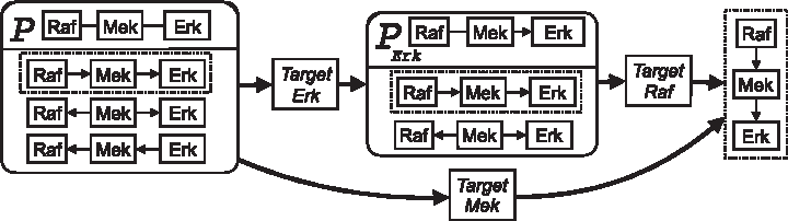
\end{document}. Imagine that the structure of the pathway is unknown and needs to be inferred. A causal inference algorithm would (1) detect pairwise statistical correlations between abundances of each pair of the three proteins, pointing to the three candidate edges, (2) test Raf and Erk for conditional independence, given the state of Mek, and (3) in the presence of conditional independence eliminate the edge between Raf and Erk. After that, additional interventions are required to orient the edges between Raf and Mek, and between Mek and Erk. The left box shown in Figure 1 illustrates that, in the absence of interventions, the ground truth is statistically indistinguishable from the other two causally incorrect DAGs.
Illustration of DAG equivalence classes. The DAG \documentclass{aastex}\usepackage{amsbsy}\usepackage{amsfonts}\usepackage{amssymb}\usepackage{bm}\usepackage{mathrsfs}\usepackage{pifont}\usepackage{stmaryrd}\usepackage{textcomp}\usepackage{portland, xspace}\usepackage{amsmath, amsxtra}\usepackage{upgreek}\pagestyle{empty}\DeclareMathSizes{10}{9}{7}{6}\begin{document}
$${Raf} \to {Mek} \to {Erk}$$
\end{document} is the “ground truth” canonical MAPK signaling pathway, which we seek to learn by causal inference. The left box shows the equivalence class P, represented by the PDAG \documentclass{aastex}\usepackage{amsbsy}\usepackage{amsfonts}\usepackage{amssymb}\usepackage{bm}\usepackage{mathrsfs}\usepackage{pifont}\usepackage{stmaryrd}\usepackage{textcomp}\usepackage{portland, xspace}\usepackage{amsmath, amsxtra}\usepackage{upgreek}\pagestyle{empty}\DeclareMathSizes{10}{9}{7}{6}\begin{document}
$${Raf} - {Mek} - {Erk}$$
\end{document}. The PDAG contains three DAGs, all statistically indistinguishable in the absence of interventions. The cardinality of P is 3. The middle box shows the PDAG \documentclass{aastex}\usepackage{amsbsy}\usepackage{amsfonts}\usepackage{amssymb}\usepackage{bm}\usepackage{mathrsfs}\usepackage{pifont}\usepackage{stmaryrd}\usepackage{textcomp}\usepackage{portland, xspace}\usepackage{amsmath, amsxtra}\usepackage{upgreek}\pagestyle{empty}\DeclareMathSizes{10}{9}{7}{6}\begin{document}
$${P_{Erk}}$$
\end{document}, obtained after an intervention or Erk. \documentclass{aastex}\usepackage{amsbsy}\usepackage{amsfonts}\usepackage{amssymb}\usepackage{bm}\usepackage{mathrsfs}\usepackage{pifont}\usepackage{stmaryrd}\usepackage{textcomp}\usepackage{portland, xspace}\usepackage{amsmath, amsxtra}\usepackage{upgreek}\pagestyle{empty}\DeclareMathSizes{10}{9}{7}{6}\begin{document}
$${P_{Erk}}$$
\end{document} is a subclass of P that has eliminated \documentclass{aastex}\usepackage{amsbsy}\usepackage{amsfonts}\usepackage{amssymb}\usepackage{bm}\usepackage{mathrsfs}\usepackage{pifont}\usepackage{stmaryrd}\usepackage{textcomp}\usepackage{portland, xspace}\usepackage{amsmath, amsxtra}\usepackage{upgreek}\pagestyle{empty}\DeclareMathSizes{10}{9}{7}{6}\begin{document}
$${Raf} \leftarrow {Mek} \leftarrow {Erk}$$
\end{document}. The cardinality of \documentclass{aastex}\usepackage{amsbsy}\usepackage{amsfonts}\usepackage{amssymb}\usepackage{bm}\usepackage{mathrsfs}\usepackage{pifont}\usepackage{stmaryrd}\usepackage{textcomp}\usepackage{portland, xspace}\usepackage{amsmath, amsxtra}\usepackage{upgreek}\pagestyle{empty}\DeclareMathSizes{10}{9}{7}{6}\begin{document}
$${P_{Erk}}$$
\end{document} is 2. The right box shows the single ground truth DAG obtained after an additional intervention on Raf. An alternative single intervention on Mek simultaneously compels the direction of both edges, and is more effective at discovering the ground truth. DAG, directed acyclic graph; PDAG, partially DAG.
A set of statistically indistinguishable DAGs forms a Markov equivalence class P, comprising DAGs with same edges but varying orientations, which have equal statistical likelihood for the data set (Pearl, 2000; Koller and Friedman, 2009). A Markov equivalence class is represented with a partially DAG (PDAG). The directed edges in a PDAG have the same orientation in all the DAGs in P. The undirected edges in the PDAG have varying directions in the DAGs and, therefore, represent edges with uncertain causality. Figure 1 illustrates PDAGs and DAGs in the MAPK pathway example. The cardinality of a PDAG is defined as the number of its DAGs.
Targeted interventions proceed by fixing the state of a node, such that it does not vary with that of its parents (Pearl, 2000; Eaton and Murphy, 2007; Koller and Friedman, 2009). Fixing the node introduces an additional constraint and eliminates members of the equivalence class that fail to satisfy this constraint. For example, in Figure 1, a small inhibitor fixes Erk's enzymatic activity state to “off,” such that the activity of Erk becomes independent of the state of Mek. The intervention fails to regulate the activity of Mek and, therefore, eliminates the DAG with an edge \documentclass{aastex}\usepackage{amsbsy}\usepackage{amsfonts}\usepackage{amssymb}\usepackage{bm}\usepackage{mathrsfs}\usepackage{pifont}\usepackage{stmaryrd}\usepackage{textcomp}\usepackage{portland, xspace}\usepackage{amsmath, amsxtra}\usepackage{upgreek}\pagestyle{empty}\DeclareMathSizes{10}{9}{7}{6}\begin{document}
$${Erk} \to {Mek}$$
\end{document}.
The reduced equivalence class is formally defined as a transition-sequence Markov equivalence class, that is, the equivalence class after a sequence of “transitions” (interventions) (Tian and Pearl, 2001). Each additional intervention orients more edges in a PDAG, and a sufficiently large set of interventions compels all the edges. As shown in Figure 1, interventions on Erk and Raf eliminated all but the ground truth from the equivalence class.
As the example illustrates, a batch of interventions targeting Erk and Raf would reveal the ground truth DAG. However, so would a batch containing a single intervention on Mek. The goal of this work is to identify batches of interventions, which reveal the most causality while minimizing the number of interventions they contain, and by extension the experimental complexity and cost.
2.2. Bayesian inference of causal networks
This work focuses on a Bayesian approach to learning causal PDAG representations of signaling, where experimentalists (1) start with background knowledge about the signaling network, such as likely pathways or motifs, (2) use the background knowledge to construct a prior distribution on graph structures, (3) collect experimental measurements of the signaling states of proteins, and (4) estimate a posterior distribution on structures based on the prior and the experimental measurements. The Bayesian approach is advantageous, as it reveals the “rewiring” of signaling between conditions by examining differences between the prior and the posterior distributions.
More formally, the approach uses the background knowledge \documentclass{aastex}\usepackage{amsbsy}\usepackage{amsfonts}\usepackage{amssymb}\usepackage{bm}\usepackage{mathrsfs}\usepackage{pifont}\usepackage{stmaryrd}\usepackage{textcomp}\usepackage{portland, xspace}\usepackage{amsmath, amsxtra}\usepackage{upgreek}\pagestyle{empty}\DeclareMathSizes{10}{9}{7}{6}\begin{document}
$$\delta$$
\end{document} to construct a prior probability distribution of possible DAG structures \documentclass{aastex}\usepackage{amsbsy}\usepackage{amsfonts}\usepackage{amssymb}\usepackage{bm}\usepackage{mathrsfs}\usepackage{pifont}\usepackage{stmaryrd}\usepackage{textcomp}\usepackage{portland, xspace}\usepackage{amsmath, amsxtra}\usepackage{upgreek}\pagestyle{empty}\DeclareMathSizes{10}{9}{7}{6}\begin{document}
$$\pi ( G \vert \delta )$$
\end{document} in the space of possible structures \documentclass{aastex}\usepackage{amsbsy}\usepackage{amsfonts}\usepackage{amssymb}\usepackage{bm}\usepackage{mathrsfs}\usepackage{pifont}\usepackage{stmaryrd}\usepackage{textcomp}\usepackage{portland, xspace}\usepackage{amsmath, amsxtra}\usepackage{upgreek}\pagestyle{empty}\DeclareMathSizes{10}{9}{7}{6}\begin{document}
$$\mathbb{G}$$
\end{document}. The experimentalist collects a data set D of measurements on the proteins \documentclass{aastex}\usepackage{amsbsy}\usepackage{amsfonts}\usepackage{amssymb}\usepackage{bm}\usepackage{mathrsfs}\usepackage{pifont}\usepackage{stmaryrd}\usepackage{textcomp}\usepackage{portland, xspace}\usepackage{amsmath, amsxtra}\usepackage{upgreek}\pagestyle{empty}\DeclareMathSizes{10}{9}{7}{6}\begin{document}
$$V \in G$$
\end{document}, acquired under a batch of targeted interventions S. A statistical likelihood function \documentclass{aastex}\usepackage{amsbsy}\usepackage{amsfonts}\usepackage{amssymb}\usepackage{bm}\usepackage{mathrsfs}\usepackage{pifont}\usepackage{stmaryrd}\usepackage{textcomp}\usepackage{portland, xspace}\usepackage{amsmath, amsxtra}\usepackage{upgreek}\pagestyle{empty}\DeclareMathSizes{10}{9}{7}{6}\begin{document}
$$p ( D \vert S , G )$$
\end{document} quantifies the likelihood that the observations were generated from a graph G. Finally, inference of the DAG structure relies on a posterior probability distribution \documentclass{aastex}\usepackage{amsbsy}\usepackage{amsfonts}\usepackage{amssymb}\usepackage{bm}\usepackage{mathrsfs}\usepackage{pifont}\usepackage{stmaryrd}\usepackage{textcomp}\usepackage{portland, xspace}\usepackage{amsmath, amsxtra}\usepackage{upgreek}\pagestyle{empty}\DeclareMathSizes{10}{9}{7}{6}\begin{document}
$$\pi ( G \vert D , S , \delta )$$
\end{document}\documentclass{aastex}\usepackage{amsbsy}\usepackage{amsfonts}\usepackage{amssymb}\usepackage{bm}\usepackage{mathrsfs}\usepackage{pifont}\usepackage{stmaryrd}\usepackage{textcomp}\usepackage{portland, xspace}\usepackage{amsmath, amsxtra}\usepackage{upgreek}\pagestyle{empty}\DeclareMathSizes{10}{9}{7}{6}\begin{document}
\begin{align*}
\pi ( G \vert D , S , \delta ) \propto p ( D \vert S , G ) \pi ( G \vert \delta ) . \tag{1}
\end{align*}
\end{document}
In many biological applications, inferring a single DAG with high posterior probability is not of the main interest. Instead, we are interested in local features of the graph, such as the presence of particular edges or network motifs. This is expressed through a function f on a graph that quantifies the feature of interest and through its posterior expectation \documentclass{aastex}\usepackage{amsbsy}\usepackage{amsfonts}\usepackage{amssymb}\usepackage{bm}\usepackage{mathrsfs}\usepackage{pifont}\usepackage{stmaryrd}\usepackage{textcomp}\usepackage{portland, xspace}\usepackage{amsmath, amsxtra}\usepackage{upgreek}\pagestyle{empty}\DeclareMathSizes{10}{9}{7}{6}\begin{document}
$$E \{ f \vert D , S , \delta \} $$
\end{document} across all graphs.
\documentclass{aastex}\usepackage{amsbsy}\usepackage{amsfonts}\usepackage{amssymb}\usepackage{bm}\usepackage{mathrsfs}\usepackage{pifont}\usepackage{stmaryrd}\usepackage{textcomp}\usepackage{portland, xspace}\usepackage{amsmath, amsxtra}\usepackage{upgreek}\pagestyle{empty}\DeclareMathSizes{10}{9}{7}{6}\begin{document}
\begin{align*}
E \{ f \vert D , S , \delta \} = \mathop \sum \limits_ \mathbb{G} f ( G ) \pi ( G \vert D , S , \delta ) . \tag{2}
\end{align*}
\end{document}
For example, if f is an indicator of the presence of an edge in the network, then \documentclass{aastex}\usepackage{amsbsy}\usepackage{amsfonts}\usepackage{amssymb}\usepackage{bm}\usepackage{mathrsfs}\usepackage{pifont}\usepackage{stmaryrd}\usepackage{textcomp}\usepackage{portland, xspace}\usepackage{amsmath, amsxtra}\usepackage{upgreek}\pagestyle{empty}\DeclareMathSizes{10}{9}{7}{6}\begin{document}
$$E \{ f \vert D , S , \delta \} $$
\end{document} is the posterior probability of the presence of that edge. In this work, our feature of interest quantifies the causal insight provided by an intervention.
Bayesian inference of DAG structures relies on a Bayesian scoring function\documentclass{aastex}\usepackage{amsbsy}\usepackage{amsfonts}\usepackage{amssymb}\usepackage{bm}\usepackage{mathrsfs}\usepackage{pifont}\usepackage{stmaryrd}\usepackage{textcomp}\usepackage{portland, xspace}\usepackage{amsmath, amsxtra}\usepackage{upgreek}\pagestyle{empty}\DeclareMathSizes{10}{9}{7}{6}\begin{document}
$$Score ( G , D , S , \delta )$$
\end{document} that takes as arguments a DAG, a data set quantifying protein activity, a set of interventions, and the structured prior knowledge. It returns values proportional to the posterior distribution \documentclass{aastex}\usepackage{amsbsy}\usepackage{amsfonts}\usepackage{amssymb}\usepackage{bm}\usepackage{mathrsfs}\usepackage{pifont}\usepackage{stmaryrd}\usepackage{textcomp}\usepackage{portland, xspace}\usepackage{amsmath, amsxtra}\usepackage{upgreek}\pagestyle{empty}\DeclareMathSizes{10}{9}{7}{6}\begin{document}
$$\pi ( G \vert D , S , \delta )$$
\end{document}. Algorithms searching for DAGs with high \documentclass{aastex}\usepackage{amsbsy}\usepackage{amsfonts}\usepackage{amssymb}\usepackage{bm}\usepackage{mathrsfs}\usepackage{pifont}\usepackage{stmaryrd}\usepackage{textcomp}\usepackage{portland, xspace}\usepackage{amsmath, amsxtra}\usepackage{upgreek}\pagestyle{empty}\DeclareMathSizes{10}{9}{7}{6}\begin{document}
$$Score ( G , D , S , \delta )$$
\end{document} must explore the combinatorially large search space of possible DAGs (Margaritis, 2003; Russel et al., 2003; Korb and Nicholson, 2010). For computational tractability, some algorithms approximate the posterior probabilities \documentclass{aastex}\usepackage{amsbsy}\usepackage{amsfonts}\usepackage{amssymb}\usepackage{bm}\usepackage{mathrsfs}\usepackage{pifont}\usepackage{stmaryrd}\usepackage{textcomp}\usepackage{portland, xspace}\usepackage{amsmath, amsxtra}\usepackage{upgreek}\pagestyle{empty}\DeclareMathSizes{10}{9}{7}{6}\begin{document}
$$\pi ( G \vert D , S , \delta )$$
\end{document} (see Cooper and Yoo, 1999; Koller and Friedman, 2009; and Scutari, 2013 for background, and Heckerman et al., 1995; Cooper and Yoo, 1999 for an example). Since the full search space over all possible DAGs \documentclass{aastex}\usepackage{amsbsy}\usepackage{amsfonts}\usepackage{amssymb}\usepackage{bm}\usepackage{mathrsfs}\usepackage{pifont}\usepackage{stmaryrd}\usepackage{textcomp}\usepackage{portland, xspace}\usepackage{amsmath, amsxtra}\usepackage{upgreek}\pagestyle{empty}\DeclareMathSizes{10}{9}{7}{6}\begin{document}
$$\mathbb{G}$$
\end{document} is combinatorially large, the common practice is to sample a set of DAGs from their posterior distribution through a random process such as bootstrap (Friedman et al., 1999; Imoto et al., 2002) or Markov Chain Monte Carlo (MCMC) (Friedman and Koller, 2003), and keep a sample of high scoring networks. \documentclass{aastex}\usepackage{amsbsy}\usepackage{amsfonts}\usepackage{amssymb}\usepackage{bm}\usepackage{mathrsfs}\usepackage{pifont}\usepackage{stmaryrd}\usepackage{textcomp}\usepackage{portland, xspace}\usepackage{amsmath, amsxtra}\usepackage{upgreek}\pagestyle{empty}\DeclareMathSizes{10}{9}{7}{6}\begin{document}
$$E \{ f \vert D , S , \delta \} $$
\end{document} is then approximated as
\documentclass{aastex}\usepackage{amsbsy}\usepackage{amsfonts}\usepackage{amssymb}\usepackage{bm}\usepackage{mathrsfs}\usepackage{pifont}\usepackage{stmaryrd}\usepackage{textcomp}\usepackage{portland, xspace}\usepackage{amsmath, amsxtra}\usepackage{upgreek}\pagestyle{empty}\DeclareMathSizes{10}{9}{7}{6}\begin{document}
\begin{align*}
E \ { f \vert D , S , \delta \ } \approx \mathop \sum \limits_ { G \in \Omega } f ( G ) { \frac { Score ( G , D , S , \delta ) } { \sum \nolimits_ { G;G \in \Omega } { Score ( G , D , S , \delta ) } } } , \tag { 3 }
\end{align*}
\end{document}
where \documentclass{aastex}\usepackage{amsbsy}\usepackage{amsfonts}\usepackage{amssymb}\usepackage{bm}\usepackage{mathrsfs}\usepackage{pifont}\usepackage{stmaryrd}\usepackage{textcomp}\usepackage{portland, xspace}\usepackage{amsmath, amsxtra}\usepackage{upgreek}\pagestyle{empty}\DeclareMathSizes{10}{9}{7}{6}\begin{document}
$$\Omega$$
\end{document} denotes a sample of high scoring DAGs.
2.3. PDAG representation of uncertainty in causal effects
Experiments with incomplete sets of interventions lack information to fully infer the causal orientation of the edges in a DAG. To characterize this uncertainty, algorithms take a single DAG and determine the space of DAGs having the same conditional independence structure, topology and likelihood \documentclass{aastex}\usepackage{amsbsy}\usepackage{amsfonts}\usepackage{amssymb}\usepackage{bm}\usepackage{mathrsfs}\usepackage{pifont}\usepackage{stmaryrd}\usepackage{textcomp}\usepackage{portland, xspace}\usepackage{amsmath, amsxtra}\usepackage{upgreek}\pagestyle{empty}\DeclareMathSizes{10}{9}{7}{6}\begin{document}
$$p ( D \vert S , G )$$
\end{document}, but different edge orientations as the input DAG (Chickering, 1995; Tian and Pearl, 2001). These DAGs form a Markov equivalence class. The algorithms return a PDAG, which represents the class by preserving the shared edge structure, while presenting edges with conflicting orientations as undirected.
In Bayesian inference of causal networks, we are interested in Markov equivalent graphs with not only the same likelihood but also the same posterior probability and the same score \documentclass{aastex}\usepackage{amsbsy}\usepackage{amsfonts}\usepackage{amssymb}\usepackage{bm}\usepackage{mathrsfs}\usepackage{pifont}\usepackage{stmaryrd}\usepackage{textcomp}\usepackage{portland, xspace}\usepackage{amsmath, amsxtra}\usepackage{upgreek}\pagestyle{empty}\DeclareMathSizes{10}{9}{7}{6}\begin{document}
$$Score ( G , D , S , \delta )$$
\end{document} (Chickering, 1995). As seen from Equation (1), Markov equivalent graphs have the same posterior only if they have the same prior probability \documentclass{aastex}\usepackage{amsbsy}\usepackage{amsfonts}\usepackage{amssymb}\usepackage{bm}\usepackage{mathrsfs}\usepackage{pifont}\usepackage{stmaryrd}\usepackage{textcomp}\usepackage{portland, xspace}\usepackage{amsmath, amsxtra}\usepackage{upgreek}\pagestyle{empty}\DeclareMathSizes{10}{9}{7}{6}\begin{document}
$$\pi ( G \vert \delta )$$
\end{document}. This last condition does not hold when the prior probabilities encode available causal information, such that for some edges orientation in one direction is more probable than the other. A contribution of this article is an implementation of a DAG-to-PDAG conversion algorithm that accounts for informative prior probabilities of causal direction of edges, and outputs a PDAG representing a class of DAGs that are Markov equivalent and have the same posterior and score.
2.4. Active learning for the optimal design of causal network inference experiments
In the context of causal inference from experiments, active learning is the task of including targeted interventions in the design to optimize the inference of edge orientation. For example, as shown in Figure 1, an intervention on Mek compels both edges in the graph and is thus more valuable than an intervention on Erk, which only orients one edge.
Previous work used active learning to distinguish members of statistically equivalent graphs (Tian and Pearl, 2001; Pournara and Wernisch, 2004; Meganck et al., 2006; He and Geng, 2008; Eberhardt et al., 2012). However, these approaches work with either a single PDAG or a selection of highly likely PDAGs. The approach in this article differs by working with the entire probability distribution of PDAGs, characterizing each PDAG by its posterior probability of containing the causal truth.
Alternative Bayesian approaches to active learning of causal networks also exist. Some of these require the experimentalists to represent their background knowledge in terms of topological orderings (Murphy, 2001; Tong and Koller, 2001), that is, an ordering of nodes such that the “from” node for every edge occurs earlier in the ordering of the “to” node. Cho et al. (2016) use Gaussian Bayesian networks with a normal-inverse gamma prior. In contrast, this article represents background knowledge in terms of probabilities of edge presence and orientation. This more intuitive approach simplifies the experimentalists' work with pathways. The proposed active learning approach also works with Gaussian continuous, discrete, and general structural assumptions on the Bayesian network joint probability distribution.
Finally, the proposed approach is similar in spirit to other methods in the bioinformatics literature that use historic data to inform experimental design. For example, Rossel and Muller (2013) used a sequential Bayesian method to plan sample size. Guan et al. (2010) used available data to find optimal orderings of high-throughput experiments. King et al. (2004) constructed a “robot scientist” that applied an active-learning strategy to functional genomics. To our knowledge, this article is the first to apply active learning to inferring the structure of cell signaling pathways.
3. Methodology
3.1. Prior knowledge for causal graph structure learning
3.1.1. Quantifying causal knowledge with edge probabilities
We propose to use probabilities of edge presence and edge orientation as a means of modeling signaling events. A set of signaling proteins, represented by nodes in V, has up to \documentclass{aastex}\usepackage{amsbsy}\usepackage{amsfonts}\usepackage{amssymb}\usepackage{bm}\usepackage{mathrsfs}\usepackage{pifont}\usepackage{stmaryrd}\usepackage{textcomp}\usepackage{portland, xspace}\usepackage{amsmath, amsxtra}\usepackage{upgreek}\pagestyle{empty}\DeclareMathSizes{10}{9}{7}{6}\begin{document}
$$ \frac { { \vert V \vert ( \vert V \vert - 1 ) } } { 2 } $$
\end{document} possible edges. Presence probability of an edge between nodes \documentclass{aastex}\usepackage{amsbsy}\usepackage{amsfonts}\usepackage{amssymb}\usepackage{bm}\usepackage{mathrsfs}\usepackage{pifont}\usepackage{stmaryrd}\usepackage{textcomp}\usepackage{portland, xspace}\usepackage{amsmath, amsxtra}\usepackage{upgreek}\pagestyle{empty}\DeclareMathSizes{10}{9}{7}{6}\begin{document}
$$\{ u , v \} $$
\end{document}, denoted \documentclass{aastex}\usepackage{amsbsy}\usepackage{amsfonts}\usepackage{amssymb}\usepackage{bm}\usepackage{mathrsfs}\usepackage{pifont}\usepackage{stmaryrd}\usepackage{textcomp}\usepackage{portland, xspace}\usepackage{amsmath, amsxtra}\usepackage{upgreek}\pagestyle{empty}\DeclareMathSizes{10}{9}{7}{6}\begin{document}
$$P ( u - v )$$
\end{document} or \documentclass{aastex}\usepackage{amsbsy}\usepackage{amsfonts}\usepackage{amssymb}\usepackage{bm}\usepackage{mathrsfs}\usepackage{pifont}\usepackage{stmaryrd}\usepackage{textcomp}\usepackage{portland, xspace}\usepackage{amsmath, amsxtra}\usepackage{upgreek}\pagestyle{empty}\DeclareMathSizes{10}{9}{7}{6}\begin{document}
$${ \overline \pi _{uv}}$$
\end{document} as a shorthand, quantifies the confidence that the edge is present in G. Orientation probability for the edge from u to v, denoted \documentclass{aastex}\usepackage{amsbsy}\usepackage{amsfonts}\usepackage{amssymb}\usepackage{bm}\usepackage{mathrsfs}\usepackage{pifont}\usepackage{stmaryrd}\usepackage{textcomp}\usepackage{portland, xspace}\usepackage{amsmath, amsxtra}\usepackage{upgreek}\pagestyle{empty}\DeclareMathSizes{10}{9}{7}{6}\begin{document}
$$P ( u \to v \vert u - v )$$
\end{document} or \documentclass{aastex}\usepackage{amsbsy}\usepackage{amsfonts}\usepackage{amssymb}\usepackage{bm}\usepackage{mathrsfs}\usepackage{pifont}\usepackage{stmaryrd}\usepackage{textcomp}\usepackage{portland, xspace}\usepackage{amsmath, amsxtra}\usepackage{upgreek}\pagestyle{empty}\DeclareMathSizes{10}{9}{7}{6}\begin{document}
$${ \overrightarrow \pi _{uv}}$$
\end{document} as a shorthand, is the conditional probability of this orientation, given that the edge is present. Since only two orientations are possible, \documentclass{aastex}\usepackage{amsbsy}\usepackage{amsfonts}\usepackage{amssymb}\usepackage{bm}\usepackage{mathrsfs}\usepackage{pifont}\usepackage{stmaryrd}\usepackage{textcomp}\usepackage{portland, xspace}\usepackage{amsmath, amsxtra}\usepackage{upgreek}\pagestyle{empty}\DeclareMathSizes{10}{9}{7}{6}\begin{document}
$$P ( u \to v \vert u - v ) = 1 - P ( u \leftarrow v \vert u - v )$$
\end{document}. The goal of targeted interventions is to resolve the orientations of the edges, that is, coerce orientation probabilities toward 0 or 1.
Let \documentclass{aastex}\usepackage{amsbsy}\usepackage{amsfonts}\usepackage{amssymb}\usepackage{bm}\usepackage{mathrsfs}\usepackage{pifont}\usepackage{stmaryrd}\usepackage{textcomp}\usepackage{portland, xspace}\usepackage{amsmath, amsxtra}\usepackage{upgreek}\pagestyle{empty}\DeclareMathSizes{10}{9}{7}{6}\begin{document}
$$\delta$$
\end{document} be a set of edge probabilities \documentclass{aastex}\usepackage{amsbsy}\usepackage{amsfonts}\usepackage{amssymb}\usepackage{bm}\usepackage{mathrsfs}\usepackage{pifont}\usepackage{stmaryrd}\usepackage{textcomp}\usepackage{portland, xspace}\usepackage{amsmath, amsxtra}\usepackage{upgreek}\pagestyle{empty}\DeclareMathSizes{10}{9}{7}{6}\begin{document}
$${ \delta _{u , v}}$$
\end{document}, where
\documentclass{aastex}\usepackage{amsbsy}\usepackage{amsfonts}\usepackage{amssymb}\usepackage{bm}\usepackage{mathrsfs}\usepackage{pifont}\usepackage{stmaryrd}\usepackage{textcomp}\usepackage{portland, xspace}\usepackage{amsmath, amsxtra}\usepackage{upgreek}\pagestyle{empty}\DeclareMathSizes{10}{9}{7}{6}\begin{document}
\begin{align*}
{ \delta _{u , v}} \mathop = \limits^{{ \rm{def}}} \{ { \overline \pi _{uv}} , { \overrightarrow \pi _{uv}} \} . \tag{4}
\end{align*}
\end{document}
In Bayesian setting, we wish to use the edge probabilities to quantify prior causal knowledge. Let \documentclass{aastex}\usepackage{amsbsy}\usepackage{amsfonts}\usepackage{amssymb}\usepackage{bm}\usepackage{mathrsfs}\usepackage{pifont}\usepackage{stmaryrd}\usepackage{textcomp}\usepackage{portland, xspace}\usepackage{amsmath, amsxtra}\usepackage{upgreek}\pagestyle{empty}\DeclareMathSizes{10}{9}{7}{6}\begin{document}
$${ \overline I _{uv}} ( G )$$
\end{document} be an indicator function for the presence of an edge between u and v in G, and \documentclass{aastex}\usepackage{amsbsy}\usepackage{amsfonts}\usepackage{amssymb}\usepackage{bm}\usepackage{mathrsfs}\usepackage{pifont}\usepackage{stmaryrd}\usepackage{textcomp}\usepackage{portland, xspace}\usepackage{amsmath, amsxtra}\usepackage{upgreek}\pagestyle{empty}\DeclareMathSizes{10}{9}{7}{6}\begin{document}
$${ \overrightarrow I _{uv}} ( G )$$
\end{document} be an indicator function for the orientation of the edge from u to v. We map edge probabilities \documentclass{aastex}\usepackage{amsbsy}\usepackage{amsfonts}\usepackage{amssymb}\usepackage{bm}\usepackage{mathrsfs}\usepackage{pifont}\usepackage{stmaryrd}\usepackage{textcomp}\usepackage{portland, xspace}\usepackage{amsmath, amsxtra}\usepackage{upgreek}\pagestyle{empty}\DeclareMathSizes{10}{9}{7}{6}\begin{document}
$$\delta$$
\end{document} to a probability distribution on DAG structures using an edge-wise prior\documentclass{aastex}\usepackage{amsbsy}\usepackage{amsfonts}\usepackage{amssymb}\usepackage{bm}\usepackage{mathrsfs}\usepackage{pifont}\usepackage{stmaryrd}\usepackage{textcomp}\usepackage{portland, xspace}\usepackage{amsmath, amsxtra}\usepackage{upgreek}\pagestyle{empty}\DeclareMathSizes{10}{9}{7}{6}\begin{document}
\begin{align*}
\pi ( G \vert \delta ) = c \prod \limits_{uv \in G} { ( 1 - { \overline \pi _{uv}} ) ^{1 - {{ \overline { I} }_{uv}} ( G ) }}{ ( { \overline \pi _{uv}}{ \overrightarrow \pi _{uv}} ) ^{{{ \overline { I} }_{uv}} ( G ) {{ \overrightarrow I }_{uv}} ( G ) }} , \tag{5}
\end{align*}
\end{document}
where c is a normalizing function on the space of graphs that corrects for the acyclicity constraint (Castelo and Siebes, 2000).
When nothing is known about the presence or orientation of the edges, we specify the uninformative edge probabilities (Scutari, 2013), where
\documentclass{aastex}\usepackage{amsbsy}\usepackage{amsfonts}\usepackage{amssymb}\usepackage{bm}\usepackage{mathrsfs}\usepackage{pifont}\usepackage{stmaryrd}\usepackage{textcomp}\usepackage{portland, xspace}\usepackage{amsmath, amsxtra}\usepackage{upgreek}\pagestyle{empty}\DeclareMathSizes{10}{9}{7}{6}\begin{document}
\begin{align*}
{ \overline \pi _ { uv } } \approx \frac { 1 } { 2 } + \frac { 1 } { { 2 ( \vert V \vert - 1 ) } } , \quad { \kern 1pt } { \rm and } { \kern 1pt } \quad \frac { } { rightarrow \pi _ { uv } } = \frac { 1 } { 2 } . \tag { 6 }
\end{align*}
\end{document}
The intuition behind Equation (6) is that two nodes are more likely to be linked in a small network than in a large network. Therefore, the uninformative presence probability approaches 0.5 as network size increases. The uninformative orientation probability is 0.5 for either direction. These uninformative edge-wise priors correspond to the marginal probabilities of an edge in the case when there is a uniform probability distribution on the space of graphs (Scutari, 2013).
Upon conducting an experiment with interventions S and collecting a data set D, the next step is to update the DAG probability distribution with condition-specific information in the data using Bayes rule
\documentclass{aastex}\usepackage{amsbsy}\usepackage{amsfonts}\usepackage{amssymb}\usepackage{bm}\usepackage{mathrsfs}\usepackage{pifont}\usepackage{stmaryrd}\usepackage{textcomp}\usepackage{portland, xspace}\usepackage{amsmath, amsxtra}\usepackage{upgreek}\pagestyle{empty}\DeclareMathSizes{10}{9}{7}{6}\begin{document}
\begin{align*}
\pi ( G \vert D , S , \delta ) \propto p ( D \vert S , G ) \pi ( G \vert \delta ) . \tag{7}
\end{align*}
\end{document}
Note that the Bayes rule is agnostic of the process that selected the interventions in S. S can be selected by any approach, such as applying the available inhibitors, or using the proposed active learning approach hereunder.
The updated probability distribution \documentclass{aastex}\usepackage{amsbsy}\usepackage{amsfonts}\usepackage{amssymb}\usepackage{bm}\usepackage{mathrsfs}\usepackage{pifont}\usepackage{stmaryrd}\usepackage{textcomp}\usepackage{portland, xspace}\usepackage{amsmath, amsxtra}\usepackage{upgreek}\pagestyle{empty}\DeclareMathSizes{10}{9}{7}{6}\begin{document}
$$\pi ( G \vert D , S , \delta )$$
\end{document} maps back to edge probabilities using the approach in Equation (2). Let \documentclass{aastex}\usepackage{amsbsy}\usepackage{amsfonts}\usepackage{amssymb}\usepackage{bm}\usepackage{mathrsfs}\usepackage{pifont}\usepackage{stmaryrd}\usepackage{textcomp}\usepackage{portland, xspace}\usepackage{amsmath, amsxtra}\usepackage{upgreek}\pagestyle{empty}\DeclareMathSizes{10}{9}{7}{6}\begin{document}
$$f (. )$$
\end{document} in Equation (2) be an indicator function \documentclass{aastex}\usepackage{amsbsy}\usepackage{amsfonts}\usepackage{amssymb}\usepackage{bm}\usepackage{mathrsfs}\usepackage{pifont}\usepackage{stmaryrd}\usepackage{textcomp}\usepackage{portland, xspace}\usepackage{amsmath, amsxtra}\usepackage{upgreek}\pagestyle{empty}\DeclareMathSizes{10}{9}{7}{6}\begin{document}
$${ \overline I _{uv}} ( G )$$
\end{document} for the presence, and an indicator function \documentclass{aastex}\usepackage{amsbsy}\usepackage{amsfonts}\usepackage{amssymb}\usepackage{bm}\usepackage{mathrsfs}\usepackage{pifont}\usepackage{stmaryrd}\usepackage{textcomp}\usepackage{portland, xspace}\usepackage{amsmath, amsxtra}\usepackage{upgreek}\pagestyle{empty}\DeclareMathSizes{10}{9}{7}{6}\begin{document}
$${ \overrightarrow I _{uv}} ( G )$$
\end{document} for the orientation, of an edge between nodes u and v in a DAG. Then, the updated presence and orientation probabilities of an edge after observing data D are defined as
\documentclass{aastex}\usepackage{amsbsy}\usepackage{amsfonts}\usepackage{amssymb}\usepackage{bm}\usepackage{mathrsfs}\usepackage{pifont}\usepackage{stmaryrd}\usepackage{textcomp}\usepackage{portland, xspace}\usepackage{amsmath, amsxtra}\usepackage{upgreek}\pagestyle{empty}\DeclareMathSizes{10}{9}{7}{6}\begin{document}
\begin{align*}
\begin{split}
{ \overline \pi _ { uv \vert D , S } } & = \mathop \sum \limits_
\mathbb { G } { \overline I _ { uv } } ( G ) \pi ( G \vert D , S ,
\delta ) \\ { \overrightarrow \pi _ { uv \vert D , S } } & =
\frac { 1 } { { { { \overline \pi } _ { uv } } } } \mathop \sum
\limits_ \mathbb { G } { \overrightarrow I _ { uv } } ( G ) \pi
( G \vert D , S , \delta ) .\end{split} \tag { 8 }
\end{align*}
\end{document}
In other words, these are average frequencies of edge presence and orientation over all the DAGs, weighted by the posterior probabilities of the DAGs.
3.1.2. Incorporating pathway knowledge and historic data
When prior information is available, we propose to construct informative edge probabilities \documentclass{aastex}\usepackage{amsbsy}\usepackage{amsfonts}\usepackage{amssymb}\usepackage{bm}\usepackage{mathrsfs}\usepackage{pifont}\usepackage{stmaryrd}\usepackage{textcomp}\usepackage{portland, xspace}\usepackage{amsmath, amsxtra}\usepackage{upgreek}\pagestyle{empty}\DeclareMathSizes{10}{9}{7}{6}\begin{document}
$${ \delta _{u , v}}$$
\end{document}. In the simplest case, a directed edge between u and v in the canonical pathway is viewed as a hypothesis that an edge linking these nodes is also present under the condition of interest, and is oriented from u to v. Denoting the set of edges in the canonical pathway as \documentclass{aastex}\usepackage{amsbsy}\usepackage{amsfonts}\usepackage{amssymb}\usepackage{bm}\usepackage{mathrsfs}\usepackage{pifont}\usepackage{stmaryrd}\usepackage{textcomp}\usepackage{portland, xspace}\usepackage{amsmath, amsxtra}\usepackage{upgreek}\pagestyle{empty}\DeclareMathSizes{10}{9}{7}{6}\begin{document}
$$\mathbb{K}$$
\end{document}, the background knowledge \documentclass{aastex}\usepackage{amsbsy}\usepackage{amsfonts}\usepackage{amssymb}\usepackage{bm}\usepackage{mathrsfs}\usepackage{pifont}\usepackage{stmaryrd}\usepackage{textcomp}\usepackage{portland, xspace}\usepackage{amsmath, amsxtra}\usepackage{upgreek}\pagestyle{empty}\DeclareMathSizes{10}{9}{7}{6}\begin{document}
$${ \delta _{u , v}}$$
\end{document} is defined as in Equation (4) where
\documentclass{aastex}\usepackage{amsbsy}\usepackage{amsfonts}\usepackage{amssymb}\usepackage{bm}\usepackage{mathrsfs}\usepackage{pifont}\usepackage{stmaryrd}\usepackage{textcomp}\usepackage{portland, xspace}\usepackage{amsmath, amsxtra}\usepackage{upgreek}\pagestyle{empty}\DeclareMathSizes{10}{9}{7}{6}\begin{document}
\begin{align*}
\begin{split}{ \overline \pi _{uv}} & = {\begin{cases}{ \ \sim
1} \ {{ \rm{if}} \ u - v \in \mathbb{K}} \\ { \ \sim 0} \ {{
\rm{otherwise}}} \hfill \\ \end{cases} } \\ { \overrightarrow \pi
_{uv}} & = \begin{cases} {\ \sim 1} & {{ \rm{if}} \it u - v {
\rm{is}} { \rm{oriented}} u \to \,v \in \ \mathbb{K} \vert u -
v \in \ \mathbb{K}} \\ {\ \sim 0} & {{ \rm{if}} \it u - v \;{
\rm{ is}} \;{ \rm{ oriented}} u \leftarrow v \in \ \mathbb{K}
\vert u - v \in \ \mathbb{K}}\ . \\ \end{cases} \end{split}
\tag{9}
\end{align*}
\end{document}
The notation \documentclass{aastex}\usepackage{amsbsy}\usepackage{amsfonts}\usepackage{amssymb}\usepackage{bm}\usepackage{mathrsfs}\usepackage{pifont}\usepackage{stmaryrd}\usepackage{textcomp}\usepackage{portland, xspace}\usepackage{amsmath, amsxtra}\usepackage{upgreek}\pagestyle{empty}\DeclareMathSizes{10}{9}{7}{6}\begin{document}
$$\sim 1$$
\end{document} (probability near 1) and \documentclass{aastex}\usepackage{amsbsy}\usepackage{amsfonts}\usepackage{amssymb}\usepackage{bm}\usepackage{mathrsfs}\usepackage{pifont}\usepackage{stmaryrd}\usepackage{textcomp}\usepackage{portland, xspace}\usepackage{amsmath, amsxtra}\usepackage{upgreek}\pagestyle{empty}\DeclareMathSizes{10}{9}{7}{6}\begin{document}
$$\sim 0$$
\end{document} (probability near 0) emphasizes that the Bayesian approach avoids the boundary probabilities of 0 and 1.
In some cases, experimentalists may wish to use alternative specifications. For example, in the absence of canonical pathway information, it may be inappropriate to assign \documentclass{aastex}\usepackage{amsbsy}\usepackage{amsfonts}\usepackage{amssymb}\usepackage{bm}\usepackage{mathrsfs}\usepackage{pifont}\usepackage{stmaryrd}\usepackage{textcomp}\usepackage{portland, xspace}\usepackage{amsmath, amsxtra}\usepackage{upgreek}\pagestyle{empty}\DeclareMathSizes{10}{9}{7}{6}\begin{document}
$${ \overline \pi _{uv}} \sim 0$$
\end{document} to each edge, and subjective edge probabilities may be a better choice. For edges where no assessments can be made, we use the uninformative edge probabilities in Equation (6).
In addition to incorporating prior knowledge from canonical pathways, we also seek to make use of information in historic data sets. We define historic data D0 as previous experiments, which quantified the activity of the proteins in the same network, under the same signaling conditions as the pending causal inference experiment, but lacking targeted interventions. We update the canonical knowledge \documentclass{aastex}\usepackage{amsbsy}\usepackage{amsfonts}\usepackage{amssymb}\usepackage{bm}\usepackage{mathrsfs}\usepackage{pifont}\usepackage{stmaryrd}\usepackage{textcomp}\usepackage{portland, xspace}\usepackage{amsmath, amsxtra}\usepackage{upgreek}\pagestyle{empty}\DeclareMathSizes{10}{9}{7}{6}\begin{document}
$$\pi ( G \vert \delta )$$
\end{document} with the condition-specific information in the historic data
\documentclass{aastex}\usepackage{amsbsy}\usepackage{amsfonts}\usepackage{amssymb}\usepackage{bm}\usepackage{mathrsfs}\usepackage{pifont}\usepackage{stmaryrd}\usepackage{textcomp}\usepackage{portland, xspace}\usepackage{amsmath, amsxtra}\usepackage{upgreek}\pagestyle{empty}\DeclareMathSizes{10}{9}{7}{6}\begin{document}
\begin{align*}
\pi ( G \vert {D_0} , \delta ) \propto p ( {D_0} \vert G ) \pi ( G \vert \delta ) . \tag{10}
\end{align*}
\end{document}
Here \documentclass{aastex}\usepackage{amsbsy}\usepackage{amsfonts}\usepackage{amssymb}\usepackage{bm}\usepackage{mathrsfs}\usepackage{pifont}\usepackage{stmaryrd}\usepackage{textcomp}\usepackage{portland, xspace}\usepackage{amsmath, amsxtra}\usepackage{upgreek}\pagestyle{empty}\DeclareMathSizes{10}{9}{7}{6}\begin{document}
$$p ( {D_0} \vert G )$$
\end{document} is the likelihood that the historic data came from graph G, and \documentclass{aastex}\usepackage{amsbsy}\usepackage{amsfonts}\usepackage{amssymb}\usepackage{bm}\usepackage{mathrsfs}\usepackage{pifont}\usepackage{stmaryrd}\usepackage{textcomp}\usepackage{portland, xspace}\usepackage{amsmath, amsxtra}\usepackage{upgreek}\pagestyle{empty}\DeclareMathSizes{10}{9}{7}{6}\begin{document}
$$\pi ( G \vert {D_0} , \delta )$$
\end{document} is the updated distribution on graph structures, which now captures the full state of our prior information before the interventions.
3.1.3. Sampling DAGS from a DAG distribution
Similar to Equations (2) and (3), the proposed Bayesian inference on causal networks relies on sampling a set of DAGs \documentclass{aastex}\usepackage{amsbsy}\usepackage{amsfonts}\usepackage{amssymb}\usepackage{bm}\usepackage{mathrsfs}\usepackage{pifont}\usepackage{stmaryrd}\usepackage{textcomp}\usepackage{portland, xspace}\usepackage{amsmath, amsxtra}\usepackage{upgreek}\pagestyle{empty}\DeclareMathSizes{10}{9}{7}{6}\begin{document}
$$\Omega$$
\end{document} from a distribution \documentclass{aastex}\usepackage{amsbsy}\usepackage{amsfonts}\usepackage{amssymb}\usepackage{bm}\usepackage{mathrsfs}\usepackage{pifont}\usepackage{stmaryrd}\usepackage{textcomp}\usepackage{portland, xspace}\usepackage{amsmath, amsxtra}\usepackage{upgreek}\pagestyle{empty}\DeclareMathSizes{10}{9}{7}{6}\begin{document}
$$\pi ( G \vert D , S , \delta )$$
\end{document}. Our implementation uses Bayesian bootstrap sampling from a distribution of DAGs (Friedman et al., 1999; Imoto et al., 2002) with random graph starts (Ide and Cozman, 2002) and greedy search, and the posterior distributions are derived using Bayesian Dirichlet approximation (Heckerman et al., 1995). When the signal-to-noise ratio in the historic data is high and/or the edge-wise prior is informative, the sampling concentrates on a smaller set of most probable DAGs. When the signal-to-noise ratio is low, weight is distributed more evenly among graphs, and the sampling must cover a larger number of graphs with similar \documentclass{aastex}\usepackage{amsbsy}\usepackage{amsfonts}\usepackage{amssymb}\usepackage{bm}\usepackage{mathrsfs}\usepackage{pifont}\usepackage{stmaryrd}\usepackage{textcomp}\usepackage{portland, xspace}\usepackage{amsmath, amsxtra}\usepackage{upgreek}\pagestyle{empty}\DeclareMathSizes{10}{9}{7}{6}\begin{document}
$$\pi ( G \vert D , S , \delta )$$
\end{document}.
3.1.4. Representing uncertainty in causal effects with PDAGs
We incorporate the informative edge orientation probabilities in \documentclass{aastex}\usepackage{amsbsy}\usepackage{amsfonts}\usepackage{amssymb}\usepackage{bm}\usepackage{mathrsfs}\usepackage{pifont}\usepackage{stmaryrd}\usepackage{textcomp}\usepackage{portland, xspace}\usepackage{amsmath, amsxtra}\usepackage{upgreek}\pagestyle{empty}\DeclareMathSizes{10}{9}{7}{6}\begin{document}
$$\delta$$
\end{document} to express the uncertainty in edge orientation using PDAGs. We view the conversion of a DAG to a PDAG as a function f in Equations (2) and (3). Applying these equations requires that DAG members of the same equivalence class have the same posterior probability, otherwise different instances of the same PDAG would have different probabilities, that is, the same f would have different probabilities in Equation (2) and scores in Equation (3). Current conversion algorithms are not compatible with edge-wise prior probabilities.
Algorithm 1 is a DAG-to-PDAG conversion algorithm that incorporates informative edge-wise prior probabilities. It starts with a DAG from \documentclass{aastex}\usepackage{amsbsy}\usepackage{amsfonts}\usepackage{amssymb}\usepackage{bm}\usepackage{mathrsfs}\usepackage{pifont}\usepackage{stmaryrd}\usepackage{textcomp}\usepackage{portland, xspace}\usepackage{amsmath, amsxtra}\usepackage{upgreek}\pagestyle{empty}\DeclareMathSizes{10}{9}{7}{6}\begin{document}
$$\Omega$$
\end{document}. Next, every directed edge is converted to an undirected edge if it meets three conditions. The first two conditions are the same as in the literature (Chickering, 1995; Tian and Pearl, 2001). First (lines 4 and 10 in Algorithm 1), reversing edge direction should not change the number of immoral v-structures (i.e., three-node motifs with one child and two parents, with no edge between parents). Second (line 6 of Algorithm 1), the child node of the edge should not be targeted by an intervention in S. In this article we introduce a third condition (line 8 in Algorithm 1), stating that the edge should have an uninformative prior orientation probability of 0.5. These conditions create an equivalence class P and its PDAG, where all the members have the same value for \documentclass{aastex}\usepackage{amsbsy}\usepackage{amsfonts}\usepackage{amssymb}\usepackage{bm}\usepackage{mathrsfs}\usepackage{pifont}\usepackage{stmaryrd}\usepackage{textcomp}\usepackage{portland, xspace}\usepackage{amsmath, amsxtra}\usepackage{upgreek}\pagestyle{empty}\DeclareMathSizes{10}{9}{7}{6}\begin{document}
$$\pi ( G \vert {D_0} , \delta )$$
\end{document}. If the algorithm is applied to two Markov equivalent DAGs with different causal information in their informative edge-wise priors, two different PDAGs are returned.
DAG to PDAG algorithm
Inputs: A DAG G, an (optional) set of selected intervention targets S, and a set of edge probabilities δ.
3.2. Bayesian active learning with causal information gain
3.2.1. Overview
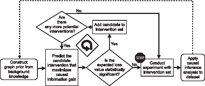
The strategy for selecting optimal interventions is overviewed in Figure 2. The active learning algorithm takes as input a sample of DAGs from a DAG distribution, and a set of candidate interventions. The algorithm sequentially evaluates the expected causal information gain of the interventions and outputs a minimally sized batch of interventions that maximizes the expected information gain. We detail the components of the algorithm hereunder.
Overview of the proposed method. A probability distribution of possible graph structures is constructed from canonical pathways and historic data. Interventions are iteratively added to the design until the expected causal information gain we can expect from an additional intervention becomes small. We then stop adding interventions to the design and use the newly acquired data to infer the causal network.
3.2.2. Defining the causal information gain of an intervention
Suppose that the true causal DAG G were known. Let \documentclass{aastex}\usepackage{amsbsy}\usepackage{amsfonts}\usepackage{amssymb}\usepackage{bm}\usepackage{mathrsfs}\usepackage{pifont}\usepackage{stmaryrd}\usepackage{textcomp}\usepackage{portland, xspace}\usepackage{amsmath, amsxtra}\usepackage{upgreek}\pagestyle{empty}\DeclareMathSizes{10}{9}{7}{6}\begin{document}
$$S \subseteq V$$
\end{document} denote a batch of candidate interventions. As discussed in Section 2.3, a PDAG is derived directly from a DAG's topology and a set of interventions, and can be determined before collecting data. Therefore, we could devise an algorithm \documentclass{aastex}\usepackage{amsbsy}\usepackage{amsfonts}\usepackage{amssymb}\usepackage{bm}\usepackage{mathrsfs}\usepackage{pifont}\usepackage{stmaryrd}\usepackage{textcomp}\usepackage{portland, xspace}\usepackage{amsmath, amsxtra}\usepackage{upgreek}\pagestyle{empty}\DeclareMathSizes{10}{9}{7}{6}\begin{document}
$$H ( G , S )$$
\end{document} that first determines a PDAG then counts the number of oriented edges in the PDAG, that is, the number of oriented edges in G that could be inferred from data with interventions S.
Suppose that we consider an additional intervention on node v, which leads to \documentclass{aastex}\usepackage{amsbsy}\usepackage{amsfonts}\usepackage{amssymb}\usepackage{bm}\usepackage{mathrsfs}\usepackage{pifont}\usepackage{stmaryrd}\usepackage{textcomp}\usepackage{portland, xspace}\usepackage{amsmath, amsxtra}\usepackage{upgreek}\pagestyle{empty}\DeclareMathSizes{10}{9}{7}{6}\begin{document}
$$H ( G , \{ S , v \} )$$
\end{document} correctly oriented edges. We define the causal information gain\documentclass{aastex}\usepackage{amsbsy}\usepackage{amsfonts}\usepackage{amssymb}\usepackage{bm}\usepackage{mathrsfs}\usepackage{pifont}\usepackage{stmaryrd}\usepackage{textcomp}\usepackage{portland, xspace}\usepackage{amsmath, amsxtra}\usepackage{upgreek}\pagestyle{empty}\DeclareMathSizes{10}{9}{7}{6}\begin{document}
$$IG ( G , S , v )$$
\end{document} of the intervention on v as the increase in correctly oriented edges, that is, \documentclass{aastex}\usepackage{amsbsy}\usepackage{amsfonts}\usepackage{amssymb}\usepackage{bm}\usepackage{mathrsfs}\usepackage{pifont}\usepackage{stmaryrd}\usepackage{textcomp}\usepackage{portland, xspace}\usepackage{amsmath, amsxtra}\usepackage{upgreek}\pagestyle{empty}\DeclareMathSizes{10}{9}{7}{6}\begin{document}
$$IG ( G , S , v ) = H ( G , \{ S , v \} ) - H ( G , S )$$
\end{document}. \documentclass{aastex}\usepackage{amsbsy}\usepackage{amsfonts}\usepackage{amssymb}\usepackage{bm}\usepackage{mathrsfs}\usepackage{pifont}\usepackage{stmaryrd}\usepackage{textcomp}\usepackage{portland, xspace}\usepackage{amsmath, amsxtra}\usepackage{upgreek}\pagestyle{empty}\DeclareMathSizes{10}{9}{7}{6}\begin{document}
$$IG ( G , S , v )$$
\end{document} is non-negative, and can be 0 if v fails to orient any edges beyond those oriented by S. Note that an equivalent definition of information gain is the reduction in the number or unoriented edges. This definition parallels the information theory notation of entropy, where the information gain is viewed as entropy reduction.
3.2.3. Selecting interventions that maximize the expected information gain
Of course in practice the true causal DAG G is unknown. Therefore, similar to Equation (2) we consider the expected information gain, which averages the information gain over all possible graphs, weighted by their prior distribution \documentclass{aastex}\usepackage{amsbsy}\usepackage{amsfonts}\usepackage{amssymb}\usepackage{bm}\usepackage{mathrsfs}\usepackage{pifont}\usepackage{stmaryrd}\usepackage{textcomp}\usepackage{portland, xspace}\usepackage{amsmath, amsxtra}\usepackage{upgreek}\pagestyle{empty}\DeclareMathSizes{10}{9}{7}{6}\begin{document}
$$\pi ( G \vert {D_0} , \delta )$$
\end{document}\documentclass{aastex}\usepackage{amsbsy}\usepackage{amsfonts}\usepackage{amssymb}\usepackage{bm}\usepackage{mathrsfs}\usepackage{pifont}\usepackage{stmaryrd}\usepackage{textcomp}\usepackage{portland, xspace}\usepackage{amsmath, amsxtra}\usepackage{upgreek}\pagestyle{empty}\DeclareMathSizes{10}{9}{7}{6}\begin{document}
\begin{align*}
EI{G_{S , v}} = \mathop \sum \limits_ \mathbb{G} IG ( G , S , v ) \pi ( G \vert {D_0} , \delta ). \tag{11}
\end{align*}
\end{document}
Moreover, similar to Equation (3), we approximate the expected information gain as
\documentclass{aastex}\usepackage{amsbsy}\usepackage{amsfonts}\usepackage{amssymb}\usepackage{bm}\usepackage{mathrsfs}\usepackage{pifont}\usepackage{stmaryrd}\usepackage{textcomp}\usepackage{portland, xspace}\usepackage{amsmath, amsxtra}\usepackage{upgreek}\pagestyle{empty}\DeclareMathSizes{10}{9}{7}{6}\begin{document}
\begin{align*}
EI { G_ { S , v } } \approx \mathop \sum \limits_ { G \in \Omega } IG ( G , S , v ) { \frac { Score ( G , { D_0 } , S , v , \delta ) } { \sum \nolimits_ { G;G \in \Omega } { Score ( G , { D_0 } , S , v , \delta ) } } } , \tag { 12 }
\end{align*}
\end{document}
where \documentclass{aastex}\usepackage{amsbsy}\usepackage{amsfonts}\usepackage{amssymb}\usepackage{bm}\usepackage{mathrsfs}\usepackage{pifont}\usepackage{stmaryrd}\usepackage{textcomp}\usepackage{portland, xspace}\usepackage{amsmath, amsxtra}\usepackage{upgreek}\pagestyle{empty}\DeclareMathSizes{10}{9}{7}{6}\begin{document}
$$\Omega$$
\end{document} denotes a sample of high-scoring DAGs, and Score is a Bayesian scoring function returning a value proportional to \documentclass{aastex}\usepackage{amsbsy}\usepackage{amsfonts}\usepackage{amssymb}\usepackage{bm}\usepackage{mathrsfs}\usepackage{pifont}\usepackage{stmaryrd}\usepackage{textcomp}\usepackage{portland, xspace}\usepackage{amsmath, amsxtra}\usepackage{upgreek}\pagestyle{empty}\DeclareMathSizes{10}{9}{7}{6}\begin{document}
$$\pi ( G \vert {D_0} , \delta )$$
\end{document}. We then select the candidate v that maximizes the approximated expected information gain. Algorithm 2 details these steps. Note that in Bayesian decision theory, \documentclass{aastex}\usepackage{amsbsy}\usepackage{amsfonts}\usepackage{amssymb}\usepackage{bm}\usepackage{mathrsfs}\usepackage{pifont}\usepackage{stmaryrd}\usepackage{textcomp}\usepackage{portland, xspace}\usepackage{amsmath, amsxtra}\usepackage{upgreek}\pagestyle{empty}\DeclareMathSizes{10}{9}{7}{6}\begin{document}
$$- IG$$
\end{document} is a loss function and we select the candidate v that minimizes the expected loss (Berger, 2013).
Expected information gain
Inputs: A set of DAGs \documentclass{aastex}\usepackage{amsbsy}\usepackage{amsfonts}\usepackage{amssymb}\usepackage{bm}\usepackage{mathrsfs}\usepackage{pifont}\usepackage{stmaryrd}\usepackage{textcomp}\usepackage{portland, xspace}\usepackage{amsmath, amsxtra}\usepackage{upgreek}\pagestyle{empty}\DeclareMathSizes{10}{9}{7}{6}\begin{document}
$$\Omega$$
\end{document}, Bayesian scoring function Score, a set of preselected intervention targets S, a candidate for next intervention v, and a set of edge probabilities \documentclass{aastex}\usepackage{amsbsy}\usepackage{amsfonts}\usepackage{amssymb}\usepackage{bm}\usepackage{mathrsfs}\usepackage{pifont}\usepackage{stmaryrd}\usepackage{textcomp}\usepackage{portland, xspace}\usepackage{amsmath, amsxtra}\usepackage{upgreek}\pagestyle{empty}\DeclareMathSizes{10}{9}{7}{6}\begin{document}
$$\delta$$
\end{document}.
3.2.4. Starting point, iterations, and stopping criteria
The proposed active learning strategy is summarized in Algorithm 3. It starts with the empty set of selected interventions \documentclass{aastex}\usepackage{amsbsy}\usepackage{amsfonts}\usepackage{amssymb}\usepackage{bm}\usepackage{mathrsfs}\usepackage{pifont}\usepackage{stmaryrd}\usepackage{textcomp}\usepackage{portland, xspace}\usepackage{amsmath, amsxtra}\usepackage{upgreek}\pagestyle{empty}\DeclareMathSizes{10}{9}{7}{6}\begin{document}
$$S = \emptyset$$
\end{document}, a set of candidate interventions U, and a set of DAGs \documentclass{aastex}\usepackage{amsbsy}\usepackage{amsfonts}\usepackage{amssymb}\usepackage{bm}\usepackage{mathrsfs}\usepackage{pifont}\usepackage{stmaryrd}\usepackage{textcomp}\usepackage{portland, xspace}\usepackage{amsmath, amsxtra}\usepackage{upgreek}\pagestyle{empty}\DeclareMathSizes{10}{9}{7}{6}\begin{document}
$$\Omega$$
\end{document}. For each intervention \documentclass{aastex}\usepackage{amsbsy}\usepackage{amsfonts}\usepackage{amssymb}\usepackage{bm}\usepackage{mathrsfs}\usepackage{pifont}\usepackage{stmaryrd}\usepackage{textcomp}\usepackage{portland, xspace}\usepackage{amsmath, amsxtra}\usepackage{upgreek}\pagestyle{empty}\DeclareMathSizes{10}{9}{7}{6}\begin{document}
$$v \in U$$
\end{document} and each DAG G in \documentclass{aastex}\usepackage{amsbsy}\usepackage{amsfonts}\usepackage{amssymb}\usepackage{bm}\usepackage{mathrsfs}\usepackage{pifont}\usepackage{stmaryrd}\usepackage{textcomp}\usepackage{portland, xspace}\usepackage{amsmath, amsxtra}\usepackage{upgreek}\pagestyle{empty}\DeclareMathSizes{10}{9}{7}{6}\begin{document}
$$\Omega$$
\end{document}, the \documentclass{aastex}\usepackage{amsbsy}\usepackage{amsfonts}\usepackage{amssymb}\usepackage{bm}\usepackage{mathrsfs}\usepackage{pifont}\usepackage{stmaryrd}\usepackage{textcomp}\usepackage{portland, xspace}\usepackage{amsmath, amsxtra}\usepackage{upgreek}\pagestyle{empty}\DeclareMathSizes{10}{9}{7}{6}\begin{document}
$${ \rm{EIG}} ( \Omega , Score , S , v )$$
\end{document} algorithm calculates PS, \documentclass{aastex}\usepackage{amsbsy}\usepackage{amsfonts}\usepackage{amssymb}\usepackage{bm}\usepackage{mathrsfs}\usepackage{pifont}\usepackage{stmaryrd}\usepackage{textcomp}\usepackage{portland, xspace}\usepackage{amsmath, amsxtra}\usepackage{upgreek}\pagestyle{empty}\DeclareMathSizes{10}{9}{7}{6}\begin{document}
$${P_{S , v}}$$
\end{document}, and \documentclass{aastex}\usepackage{amsbsy}\usepackage{amsfonts}\usepackage{amssymb}\usepackage{bm}\usepackage{mathrsfs}\usepackage{pifont}\usepackage{stmaryrd}\usepackage{textcomp}\usepackage{portland, xspace}\usepackage{amsmath, amsxtra}\usepackage{upgreek}\pagestyle{empty}\DeclareMathSizes{10}{9}{7}{6}\begin{document}
$$IG ( G , S , v )$$
\end{document}, and returns the expected information gain. The candidate with the maximum expected information gain is added to the batch S. In the next iteration, the expected information gain for the remaining candidates is evaluated, while accounting for the effect of the interventions that are already in the batch.
Active learning
Inputs: A set of DAGs \documentclass{aastex}\usepackage{amsbsy}\usepackage{amsfonts}\usepackage{amssymb}\usepackage{bm}\usepackage{mathrsfs}\usepackage{pifont}\usepackage{stmaryrd}\usepackage{textcomp}\usepackage{portland, xspace}\usepackage{amsmath, amsxtra}\usepackage{upgreek}\pagestyle{empty}\DeclareMathSizes{10}{9}{7}{6}\begin{document}
$$\Omega$$
\end{document}, Bayesian scoring function Score, a set U of candidates for next intervention, and a set of edge probabilities \documentclass{aastex}\usepackage{amsbsy}\usepackage{amsfonts}\usepackage{amssymb}\usepackage{bm}\usepackage{mathrsfs}\usepackage{pifont}\usepackage{stmaryrd}\usepackage{textcomp}\usepackage{portland, xspace}\usepackage{amsmath, amsxtra}\usepackage{upgreek}\pagestyle{empty}\DeclareMathSizes{10}{9}{7}{6}\begin{document}
$$\delta$$
\end{document}.
Parameter: \documentclass{aastex}\usepackage{amsbsy}\usepackage{amsfonts}\usepackage{amssymb}\usepackage{bm}\usepackage{mathrsfs}\usepackage{pifont}\usepackage{stmaryrd}\usepackage{textcomp}\usepackage{portland, xspace}\usepackage{amsmath, amsxtra}\usepackage{upgreek}\pagestyle{empty}\DeclareMathSizes{10}{9}{7}{6}\begin{document}
$$\alpha$$
\end{document}, stopping criterion for information gain.
12: S \documentclass{aastex}\usepackage{amsbsy}\usepackage{amsfonts}\usepackage{amssymb}\usepackage{bm}\usepackage{mathrsfs}\usepackage{pifont}\usepackage{stmaryrd}\usepackage{textcomp}\usepackage{portland, xspace}\usepackage{amsmath, amsxtra}\usepackage{upgreek}\pagestyle{empty}\DeclareMathSizes{10}{9}{7}{6}\begin{document}
$$\leftarrow$$
\end{document} cat(S, TopCandidate)
13: U \documentclass{aastex}\usepackage{amsbsy}\usepackage{amsfonts}\usepackage{amssymb}\usepackage{bm}\usepackage{mathrsfs}\usepackage{pifont}\usepackage{stmaryrd}\usepackage{textcomp}\usepackage{portland, xspace}\usepackage{amsmath, amsxtra}\usepackage{upgreek}\pagestyle{empty}\DeclareMathSizes{10}{9}{7}{6}\begin{document}
$$\leftarrow$$
\end{document} U[-TopCandidate]
14: else
15: return (S)
After a certain point, additional interventions to the batch become counterproductive. For example, as shown in Figure 1, an intervention on Mek would orient the \documentclass{aastex}\usepackage{amsbsy}\usepackage{amsfonts}\usepackage{amssymb}\usepackage{bm}\usepackage{mathrsfs}\usepackage{pifont}\usepackage{stmaryrd}\usepackage{textcomp}\usepackage{portland, xspace}\usepackage{amsmath, amsxtra}\usepackage{upgreek}\pagestyle{empty}\DeclareMathSizes{10}{9}{7}{6}\begin{document}
$$Mek - Erk$$
\end{document} edge. Including an additional intervention on Erk would provide no additional information. In the case of Figure 1, the true graph is known, and we stop adding interventions when the information gain is 0. Since in real-life situations the structure of the true DAG is unknown, we stop adding interventions when the probability that at least some information gain occurs is below a parameter \documentclass{aastex}\usepackage{amsbsy}\usepackage{amsfonts}\usepackage{amssymb}\usepackage{bm}\usepackage{mathrsfs}\usepackage{pifont}\usepackage{stmaryrd}\usepackage{textcomp}\usepackage{portland, xspace}\usepackage{amsmath, amsxtra}\usepackage{upgreek}\pagestyle{empty}\DeclareMathSizes{10}{9}{7}{6}\begin{document}
$$\alpha$$
\end{document}. Similar to Equations (3) and (12), the probability that at least some information gain occurs is
\documentclass{aastex}\usepackage{amsbsy}\usepackage{amsfonts}\usepackage{amssymb}\usepackage{bm}\usepackage{mathrsfs}\usepackage{pifont}\usepackage{stmaryrd}\usepackage{textcomp}\usepackage{portland, xspace}\usepackage{amsmath, amsxtra}\usepackage{upgreek}\pagestyle{empty}\DeclareMathSizes{10}{9}{7}{6}\begin{document}
\begin{align*}
{ q_ { S , v } } = \mathop \sum \limits_ { G \in \Omega } { I_ { \ { IG ( G , S , v ) > 0 \ } } } { \frac { Score ( G , { D_0 } , S , v , \delta ) } { \sum \nolimits_ { G \in \Omega } { Score ( G , { D_0 } , S , v , \delta ) } } } , \tag { 13 }
\end{align*}
\end{document}
where v is the candidate that maximizes expected information gain (EIG) and \documentclass{aastex}\usepackage{amsbsy}\usepackage{amsfonts}\usepackage{amssymb}\usepackage{bm}\usepackage{mathrsfs}\usepackage{pifont}\usepackage{stmaryrd}\usepackage{textcomp}\usepackage{portland, xspace}\usepackage{amsmath, amsxtra}\usepackage{upgreek}\pagestyle{empty}\DeclareMathSizes{10}{9}{7}{6}\begin{document}
$${I_{ \{ \} }}$$
\end{document} is the indicator function. We add v to the set of interventions if \documentclass{aastex}\usepackage{amsbsy}\usepackage{amsfonts}\usepackage{amssymb}\usepackage{bm}\usepackage{mathrsfs}\usepackage{pifont}\usepackage{stmaryrd}\usepackage{textcomp}\usepackage{portland, xspace}\usepackage{amsmath, amsxtra}\usepackage{upgreek}\pagestyle{empty}\DeclareMathSizes{10}{9}{7}{6}\begin{document}
$${q_{S , v}} > \alpha$$
\end{document} and stop if \documentclass{aastex}\usepackage{amsbsy}\usepackage{amsfonts}\usepackage{amssymb}\usepackage{bm}\usepackage{mathrsfs}\usepackage{pifont}\usepackage{stmaryrd}\usepackage{textcomp}\usepackage{portland, xspace}\usepackage{amsmath, amsxtra}\usepackage{upgreek}\pagestyle{empty}\DeclareMathSizes{10}{9}{7}{6}\begin{document}
$${q_{S , v}} \le \alpha$$
\end{document}. Higher values of \documentclass{aastex}\usepackage{amsbsy}\usepackage{amsfonts}\usepackage{amssymb}\usepackage{bm}\usepackage{mathrsfs}\usepackage{pifont}\usepackage{stmaryrd}\usepackage{textcomp}\usepackage{portland, xspace}\usepackage{amsmath, amsxtra}\usepackage{upgreek}\pagestyle{empty}\DeclareMathSizes{10}{9}{7}{6}\begin{document}
$$\alpha$$
\end{document} will result in a smaller intervention batch. Setting probability threshold \documentclass{aastex}\usepackage{amsbsy}\usepackage{amsfonts}\usepackage{amssymb}\usepackage{bm}\usepackage{mathrsfs}\usepackage{pifont}\usepackage{stmaryrd}\usepackage{textcomp}\usepackage{portland, xspace}\usepackage{amsmath, amsxtra}\usepackage{upgreek}\pagestyle{empty}\DeclareMathSizes{10}{9}{7}{6}\begin{document}
$$\alpha$$
\end{document} to \documentclass{aastex}\usepackage{amsbsy}\usepackage{amsfonts}\usepackage{amssymb}\usepackage{bm}\usepackage{mathrsfs}\usepackage{pifont}\usepackage{stmaryrd}\usepackage{textcomp}\usepackage{portland, xspace}\usepackage{amsmath, amsxtra}\usepackage{upgreek}\pagestyle{empty}\DeclareMathSizes{10}{9}{7}{6}\begin{document}
$$\sim 0$$
\end{document} (i.e., stopping when the probability of at least some information gain is near 0) is equivalent to stopping when expected information gain is near 0.
When the signal-to-noise ratio in the historic data is low, there is greater weight on graphs where the most optimal intervention candidates have no information gain. This leads to triggering of the stopping criteria with a smaller batch of interventions. Thus when there is more uncertainty in the data, the procedure avoids the risk of wasteful use of interventions, instead favoring running the experiment with a smaller batch and then relying on the new experimental data to evaluate unused interventions.
3.3. Inference of causal network from data acquired postintervention
The next step in the investigation is to apply the selected interventions and collect a new data set D. The new data set updates Equation (7) as
\documentclass{aastex}\usepackage{amsbsy}\usepackage{amsfonts}\usepackage{amssymb}\usepackage{bm}\usepackage{mathrsfs}\usepackage{pifont}\usepackage{stmaryrd}\usepackage{textcomp}\usepackage{portland, xspace}\usepackage{amsmath, amsxtra}\usepackage{upgreek}\pagestyle{empty}\DeclareMathSizes{10}{9}{7}{6}\begin{document}
\begin{align*}
\pi ( G \vert S , {D_0} , D , \delta ) \propto p ( D \vert S , G ) \pi ( G \vert {D_0} , \delta ). \tag{14}
\end{align*}
\end{document}
The updated edge probabilities are obtained as in Equations (8) and (9). They balance the canonical representation of the signaling with the condition-specific signaling behavior quantified under the condition of interest, after the interventions. A large deviation of the posterior edge probability from the prior in \documentclass{aastex}\usepackage{amsbsy}\usepackage{amsfonts}\usepackage{amssymb}\usepackage{bm}\usepackage{mathrsfs}\usepackage{pifont}\usepackage{stmaryrd}\usepackage{textcomp}\usepackage{portland, xspace}\usepackage{amsmath, amsxtra}\usepackage{upgreek}\pagestyle{empty}\DeclareMathSizes{10}{9}{7}{6}\begin{document}
$$\delta$$
\end{document} indicates network rewiring or deregulation.
The active learning procedure is iterative in nature, in that the results of the intervention experiment can be viewed as a new instance of historic data. They can inform the selection of new interventions by substituting \documentclass{aastex}\usepackage{amsbsy}\usepackage{amsfonts}\usepackage{amssymb}\usepackage{bm}\usepackage{mathrsfs}\usepackage{pifont}\usepackage{stmaryrd}\usepackage{textcomp}\usepackage{portland, xspace}\usepackage{amsmath, amsxtra}\usepackage{upgreek}\pagestyle{empty}\DeclareMathSizes{10}{9}{7}{6}\begin{document}
$$\pi ( G \vert S , {D_0} , D , \delta )$$
\end{document} in Equations (11) and (12) and repeating the overall procedure.
3.4. Implementation and computational complexity
The proposed strategy is implemented in an open-source R package bninfo, available on Github. The edge-wise prior is constructed as a data frame in R, either manually or through an interface to the API of KEGG provided by bninfo. Historic data are represented as a data frame and preselected interventions S as an array. The package bninfo implements the algorithms for converting a DAG and an edge-wise to PDAG, calculating the expected gain and selecting the optimal batch of interventions. The Bayesian network structure learning is performed with the existing R package bnlearn (Scutari, 2010).
The main scalability bottleneck in the proposed strategy is the selection of interventions in the while loop in Algorithm 3. The complexity of calculating the expected information gain for a single intervention (Algorithm 2 and line 7 in Algorithm 3) is in the order of the number of edges in the input DAG. However, the interventions in a batch are selected sequentially (i.e., the selection of the jth member of the batch depends on the \documentclass{aastex}\usepackage{amsbsy}\usepackage{amsfonts}\usepackage{amssymb}\usepackage{bm}\usepackage{mathrsfs}\usepackage{pifont}\usepackage{stmaryrd}\usepackage{textcomp}\usepackage{portland, xspace}\usepackage{amsmath, amsxtra}\usepackage{upgreek}\pagestyle{empty}\DeclareMathSizes{10}{9}{7}{6}\begin{document}
$$j - 1$$
\end{document} previously selected interventions). Therefore, the selection of j candidate interventions requires up to \documentclass{aastex}\usepackage{amsbsy}\usepackage{amsfonts}\usepackage{amssymb}\usepackage{bm}\usepackage{mathrsfs}\usepackage{pifont}\usepackage{stmaryrd}\usepackage{textcomp}\usepackage{portland, xspace}\usepackage{amsmath, amsxtra}\usepackage{upgreek}\pagestyle{empty}\DeclareMathSizes{10}{9}{7}{6}\begin{document}
$$j!$$
\end{document} calculations of the expected gain. The running time can be reduced by parallelization of Algorithm 2 or by limiting the number of candidate interventions. Moreover, sampling \documentclass{aastex}\usepackage{amsbsy}\usepackage{amsfonts}\usepackage{amssymb}\usepackage{bm}\usepackage{mathrsfs}\usepackage{pifont}\usepackage{stmaryrd}\usepackage{textcomp}\usepackage{portland, xspace}\usepackage{amsmath, amsxtra}\usepackage{upgreek}\pagestyle{empty}\DeclareMathSizes{10}{9}{7}{6}\begin{document}
$$\Omega$$
\end{document} from a distribution of DAGs has well-known scalability challenges in Bayesian literature. In the worst case, the computational time scales exponentially with the number of proteins. Bayesian bootstrap sampling can be split among nodes on a cluster and sped up by parallelization. For the data sets described hereunder, the generation of intervention batches took 70 minutes (17 protein DREAM4 network with 14 candidate interventions and 500 sampled graphs) and 20 minutes (11 protein T cell network with 5 candidate interventions and 500 sampled graphs) on a 16 node cluster.
3.5. Metrics used for performance evaluation
We evaluated the proposed strategy using data sets containing some notion of “ground truth,” that is, situations where the true structure of the causal graph is known. We used the proposed active learning strategy to determine an optimal intervention batch S. To evaluate the performance of S, we considered data D that would be experimentally acquired with the selected interventions. We then inferred causal networks from D and derived posterior edge probabilities as described in Section 2.2. Finally, we evaluated whether S can lead to network inference that correctly detects edges in the “ground truth” graph.
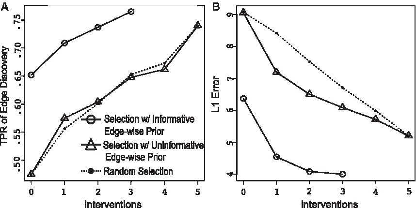
We evaluated the performance of edge detection using two metrics. The first is the true positive rate of edge detection, that is, the proportion of correctly detected edges among the edges in the ground truth network (Friedman et al., 1999). Our cutoff for edge's detection is the presence and orientation probabilities greater than uninformative prior probabilities described in Equation (6). The second metric is the L1 edge error, which quantifies the overall probability of prediction error, that is, the probability of either discovering a false edge or missing a true edge (Murphy, 2001; Tong and Koller, 2001). Given the set of interventions S and the ground truth network, the L1 edge detection error is defined as
\documentclass{aastex}\usepackage{amsbsy}\usepackage{amsfonts}\usepackage{amssymb}\usepackage{bm}\usepackage{mathrsfs}\usepackage{pifont}\usepackage{stmaryrd}\usepackage{textcomp}\usepackage{portland, xspace}\usepackage{amsmath, amsxtra}\usepackage{upgreek}\pagestyle{empty}\DeclareMathSizes{10}{9}{7}{6}\begin{document}
\begin{align*}
\begin{split} {L_1} ( G , S ) \ & = \mathop \sum \limits_{u , v} {
\overrightarrow I _{uv}} ( G ) ( 1 - { \overrightarrow \pi _{uv
\vert D , S}} )
\\ & + ( 1 - { \overrightarrow I _{uv}} ( G ) ) ( {
\overrightarrow \pi _{uv \vert D , S}} ) \\ & + ( 1 - { \overline
I _{uv}} ( G ) ) ( { \overline \pi _{uv \vert D , S}} )
\quad\quad\quad ,
\\ \end{split}
\tag{15}
\end{align*}
\end{document}
where \documentclass{aastex}\usepackage{amsbsy}\usepackage{amsfonts}\usepackage{amssymb}\usepackage{bm}\usepackage{mathrsfs}\usepackage{pifont}\usepackage{stmaryrd}\usepackage{textcomp}\usepackage{portland, xspace}\usepackage{amsmath, amsxtra}\usepackage{upgreek}\pagestyle{empty}\DeclareMathSizes{10}{9}{7}{6}\begin{document}
$${ \overrightarrow I _{uv}} ( G )$$
\end{document} and \documentclass{aastex}\usepackage{amsbsy}\usepackage{amsfonts}\usepackage{amssymb}\usepackage{bm}\usepackage{mathrsfs}\usepackage{pifont}\usepackage{stmaryrd}\usepackage{textcomp}\usepackage{portland, xspace}\usepackage{amsmath, amsxtra}\usepackage{upgreek}\pagestyle{empty}\DeclareMathSizes{10}{9}{7}{6}\begin{document}
$${ \overline I _{uv}} ( G )$$
\end{document} are as in Equation (9).
4. Data Sets
There are currently no publicly available data sets that implement active learning approach to causal network inference. We, therefore, use two publicly available data sets, adapted to provide a measure of “ground truth.”
4.1. DREAM4 Network
4.1.1. “Ground truth” network
The 17-node network shown in Figure 3A was used in the DREAM4 Predictive Signaling Network Challenge (Prill et al., 2011). The network contains canonical pathways downstream of four receptors (dark gray nodes shown in Fig. 3A): two inflammatory (TNFa, IL1a), one insulin (IGF-I), and one growth factor receptor (TGFa). We use this network to evaluate the relative advantages of active learning and the importance of the use of prior information.
The “ground truth” networks in the experimental data sets. (A) The DREAM4 Predictive Signaling Network Challenge network. Dark nodes indicate receptors. (B) Native T cell signaling network in response to antigen. The edges in the \documentclass{aastex}\usepackage{amsbsy}\usepackage{amsfonts}\usepackage{amssymb}\usepackage{bm}\usepackage{mathrsfs}\usepackage{pifont}\usepackage{stmaryrd}\usepackage{textcomp}\usepackage{portland, xspace}\usepackage{amsmath, amsxtra}\usepackage{upgreek}\pagestyle{empty}\DeclareMathSizes{10}{9}{7}{6}\begin{document}
$${PKC} \to {Raf} \to {Mek} \to {Erk}$$
\end{document} cascade and the edge \documentclass{aastex}\usepackage{amsbsy}\usepackage{amsfonts}\usepackage{amssymb}\usepackage{bm}\usepackage{mathrsfs}\usepackage{pifont}\usepackage{stmaryrd}\usepackage{textcomp}\usepackage{portland, xspace}\usepackage{amsmath, amsxtra}\usepackage{upgreek}\pagestyle{empty}\DeclareMathSizes{10}{9}{7}{6}\begin{document}
$${PKA} \to {Raf}$$
\end{document} belong to the canonical MAPK pathway. Dark nodes indicate targets of experimental interventions.
4.1.2. Prior information regarding the network structure
We used as the background information the fact that TNFa, IL1a, IGF-I, and TGFa are receptors, that is, proteins that receive signals from the environment and activate downstream proteins. This presents causal information, in that the remaining proteins in the pathway are downstream of the receptors.
4.1.3. Historic data
We use the DREAM4 challenge as a historic data set. The challenge provided antibody-based measurements (sandwich immunoassays with the Luminex xMAP platform) from hepatocellular carcinoma cell lines (HepG2), which quantified the activity levels of the signaling proteins at bulk (i.e., nonsingle-cell) resolution. The data set comprises samples with five stimulus conditions, namely no stimulus, stimulus on TNFa, on IL1a, on IGF1, and on TGFa. The data set also includes five intervention conditions, namely no inhibition, inhibition on ikk, on mek12, on pi3k, and on p38. In total there were 25 samples, one for each stimulus and intervention pair.
We processed the historic data set as follows. We imputed missing values using a neural network model that predicted missing values of a protein given the values of the protein's neighbors in the ground truth network. Several proteins from the pathway (map3k7, ras, map3k1, and mkk4) were not quantified in the historic data set. Approaches exist for learning Bayesian network structure with hidden variables (Chickering and Heckerman, 1997, Friedman, 1997), but these are beyond the scope of this article. So to eliminate this artifact, we applied a model that predicts a protein's values given the values of its parents in the model and common biochemical assumptions on signaling dynamics (Terfve et al., 2012) and used the model to predict the values for the hidden nodes. The publicly available challenge data are normalized to the 0–1 range, we then discretized the quantification values to binary on/off variables using 0.5 as a cutoff.
4.1.4. Candidate interventions
All the nonreceptor nodes in the network were considered as candidates for interventions. Owing to the small number of samples and inhibitions, it was not possible to set aside a portion of this data set for performance evaluation. Therefore, we fit a causal network model to the challenge data and the ground truth network and used the model fit to generate synthetic postintervention data sets. The simulation mimicked the design of the challenge data, in that it contained one biological sample for each intervention. We then evaluated the performance of the selected interventions on these synthetic data sets.
4.2. Flow cytometry measurements of T cell signaling
4.2.1. “Ground truth” network
The network shown in Figure 3B contains 11 phosphoproteins and phospholipids involved in the native CD4+ T cell signaling response to antigen and their canonical edges. The network was used to validate causal inference from an experimental data set (Sachs et al., 2005), and has been subsequently used as a benchmark in multiple causal inference studies (Eaton and Murphy, 2007; Friedman et al., 2008).
4.2.2. Prior information regarding the network structure
We used as the background knowledge the edges in the canonical MAPK pathway. Although CD4+ T cell signaling has been extensively studied, we assumed that no prior information is available regarding the remaining edges. This assumption allowed us to compare the case of a minimally informative prior the case of an uninformative prior, and focus performance evaluation on detection edges that were not addressed in the background knowledge.
4.2.3. Historic data
The experimental data set given in Sachs et al. (2005) contains single-cell fluorescence-based quantifications of 11 phosphoproteins and phospholipids in human primary naive CD4+ T cells. These analytes are downstream of the receptors CD3 and CD28 that provide costimulatory signals required for T cell activation. We used as the “historic data” a portion of this data set that was acquired without any targeted interventions. This portion of the data set contained 11,672 cells.
4.2.4. Candidate interventions
The data set given in Sachs et al. (2005) also contained single-cell quantifications, acquired after activating or inhibiting five signaling proteins (dark nodes shown in Fig. 3B). These five proteins were considered as candidates for interventions in this article. The postintervention experimental data sets were used to compare the information gain projected in our approach with the actual information gain after the interventions.
5. Results
5.1. Informative prior edge probabilities reduced the required number of interventions in the DREAM4 data set
In the DREAM4 data set, we compared (1) random ordering of interventions, (2) proposed active learning strategy with uninformative prior probabilities of edge presence [Eq. (6)], and (3) the same active learning strategy, but with informative priors. The informative priors encoded the fact that the receptor nodes have upstream positions in the network. All the receptor-originating edges were assigned the prior orientation probability of \documentclass{aastex}\usepackage{amsbsy}\usepackage{amsfonts}\usepackage{amssymb}\usepackage{bm}\usepackage{mathrsfs}\usepackage{pifont}\usepackage{stmaryrd}\usepackage{textcomp}\usepackage{portland, xspace}\usepackage{amsmath, amsxtra}\usepackage{upgreek}\pagestyle{empty}\DeclareMathSizes{10}{9}{7}{6}\begin{document}
$$\sim 1$$
\end{document}, all receptor-terminating edges were assigned the presence probability of \documentclass{aastex}\usepackage{amsbsy}\usepackage{amsfonts}\usepackage{amssymb}\usepackage{bm}\usepackage{mathrsfs}\usepackage{pifont}\usepackage{stmaryrd}\usepackage{textcomp}\usepackage{portland, xspace}\usepackage{amsmath, amsxtra}\usepackage{upgreek}\pagestyle{empty}\DeclareMathSizes{10}{9}{7}{6}\begin{document}
$$\sim 0$$
\end{document}, and the remaining edges were assigned the uniformed prior presence probability in Equation (6). All the nonreceptor nodes in the network were candidate targets for interventions. To exhaust the information in the prior and historic data, the active learning approach with both priors used the most liberal stopping criteria for growing a batch. It only stopped adding interventions when all the additional candidates have expected information gain of \documentclass{aastex}\usepackage{amsbsy}\usepackage{amsfonts}\usepackage{amssymb}\usepackage{bm}\usepackage{mathrsfs}\usepackage{pifont}\usepackage{stmaryrd}\usepackage{textcomp}\usepackage{portland, xspace}\usepackage{amsmath, amsxtra}\usepackage{upgreek}\pagestyle{empty}\DeclareMathSizes{10}{9}{7}{6}\begin{document}
$$\sim 0$$
\end{document}.
Figure 4 summarizes the results. With uninformative edge-wise priors, random selection of interventions performed similar to the proposed active learning in both true positive rate of edge detection and L1 loss. Both metrics depend on correct detection of edge presence as well as edge orientation. The contribution to edge detection of the added samples provided by each intervention experiment overshadowed the selection strategies prioritization of interventions that better resolve edge orientation.
Performance of the proposed strategy on the DREAM4 data set. Dotted line: uninformative edge-wise priors, randomly selected interventions. Solid line with triangles: uninformative edge-wise priors, interventions selected with active learning. Solid line with circles: informative edge-wise priors, interventions selected active learning. (A) TPR of detecting ground truth edges. (B)L1 error of detecting ground truth edges. TPR, true positive rate.
At the same time, the results demonstrate the efficiency gain in selecting the interventions, brought by encoding the knowledge of receptor identities into the prior. For example, although with the uninformative prior the true positive rate of more than 0.35 could be achieved with on average nine interventions, the informative prior only required on average 6 interventions. Table 2 shows the specific interventions that were selected at a conservative cutoff (\documentclass{aastex}\usepackage{amsbsy}\usepackage{amsfonts}\usepackage{amssymb}\usepackage{bm}\usepackage{mathrsfs}\usepackage{pifont}\usepackage{stmaryrd}\usepackage{textcomp}\usepackage{portland, xspace}\usepackage{amsmath, amsxtra}\usepackage{upgreek}\pagestyle{empty}\DeclareMathSizes{10}{9}{7}{6}\begin{document}
$${q_{S , v}} \le 0.01$$
\end{document}). The results indicate that informative edge-wise priors are important for such bulk experiments with a small number of replicate samples. The prior knowledge removed uncertainty in edge presence, increasing the contribution of improved detection of edge orientation to overall performance.
Intervention Targets Selected by Active Learning in the T Cell Data Set. The Use of an Informative Edge-Wise Prior Eliminates Two Interventions from the Batch
Prior
Intervention targets selected by active learning
Informative
(1) PKA, (2) PKC, (3) PIP2
Uninformative
(1) PKA, (2) PIP2, (3) PKC, (4) Akt, (5) Mek
5.2. The ordering of T cell interventions by active learning matched their contribution to causal inference
As already mentioned, for the T cell data set, we compared (1) random ordering of interventions, (2) proposed active learning strategy with uninformative prior probabilities of edge presence [Eq. (6)], and (3) the same active learning strategy, but with informative priors. In the latter case, we assumed the prior knowledge of the canonical MAPK pathway and assigned a high prior probability (\documentclass{aastex}\usepackage{amsbsy}\usepackage{amsfonts}\usepackage{amssymb}\usepackage{bm}\usepackage{mathrsfs}\usepackage{pifont}\usepackage{stmaryrd}\usepackage{textcomp}\usepackage{portland, xspace}\usepackage{amsmath, amsxtra}\usepackage{upgreek}\pagestyle{empty}\DeclareMathSizes{10}{9}{7}{6}\begin{document}
$$\sim 1$$
\end{document}) to the edges in the \documentclass{aastex}\usepackage{amsbsy}\usepackage{amsfonts}\usepackage{amssymb}\usepackage{bm}\usepackage{mathrsfs}\usepackage{pifont}\usepackage{stmaryrd}\usepackage{textcomp}\usepackage{portland, xspace}\usepackage{amsmath, amsxtra}\usepackage{upgreek}\pagestyle{empty}\DeclareMathSizes{10}{9}{7}{6}\begin{document}
$${PKC} \to {Raf} \to {Mek} \to {Erk}$$
\end{document} cascade and to the edge \documentclass{aastex}\usepackage{amsbsy}\usepackage{amsfonts}\usepackage{amssymb}\usepackage{bm}\usepackage{mathrsfs}\usepackage{pifont}\usepackage{stmaryrd}\usepackage{textcomp}\usepackage{portland, xspace}\usepackage{amsmath, amsxtra}\usepackage{upgreek}\pagestyle{empty}\DeclareMathSizes{10}{9}{7}{6}\begin{document}
$${PKA} \to {Raf}$$
\end{document}. The remaining potential edges were assigned the uninformative prior probability of both presence and orientation. We then considered the five interventions given in Sachs et al. (2005) as the set of candidate interventions.
Figure 5 summarizes the results. Selection with an uninformative edge-wise prior did not outperform random selection of interventions in terms of true positive rate of detecting edges. However, it had a smaller L1 error for the first three selected interventions. With this experiment, the intervention data sets served not just to resolve causality but also to improve edge detection by adding variation in signaling activity not present is preceding data sets. As with the DREAM4 data, this led to performance gains due to improved edge detection overshadowed gains owed to the selection strategy.
Performance of the proposed strategy on the T cell signaling data set. Lines and panels are as shown in Figure 4.
In contrast, active learning with the edge-wise prior encoding the MAPK edges outperformed random selection in terms of both greater true positive rate and smaller L1 error. Table 1 shows the specific interventions that were selected at a conservative cutoff \documentclass{aastex}\usepackage{amsbsy}\usepackage{amsfonts}\usepackage{amssymb}\usepackage{bm}\usepackage{mathrsfs}\usepackage{pifont}\usepackage{stmaryrd}\usepackage{textcomp}\usepackage{portland, xspace}\usepackage{amsmath, amsxtra}\usepackage{upgreek}\pagestyle{empty}\DeclareMathSizes{10}{9}{7}{6}\begin{document}
$$( {q_{S , v}} \le 0.01 )$$
\end{document}. For example, although with the uninformative prior the true positive rate of 0.75 could be achieved with on average five interventions, the informative prior only required on average three interventions.
Intervention Targets Selected by Active Learning in the DREAM4 Data Set
The informative prior edge probabilities required a smaller intervention batch.
The network structure provides some insight into the role of informative edge-wise priors in improving the performance. Since the orientation probability of an edge depends on the orientation probability of its neighbors, the edge-wise prior reduced error by reducing uncertainty in the orientation of edges neighboring the MAPK edges. In addition, the edge-wise prior enabled the causal inference procedure to down weight graphs where the MAPK edges were not present or had the wrong orientation, increasing sensitivity. Finally, additional causal information encoded in the prior made interventions on Mek and Akt interventions less useful, enabling the stopping criteria to eliminate them from the batch.
6. Conclusions
Our results showed that an active learning strategy, combined with informative priors, is the most effective at suggesting the smallest batch of target interventions for inference of causal networks. It optimizes the causal information in the intervention experiments, while controlling the experiment time and cost.
The background information comes in the form of prior knowledge on the presence and orientation of edges in the system available, for example, in pathway databases such as KEGG, as well as from historic data sets available, for example, from repositories such as Cytobank. The proposed strategy can be used with any level of prior information or uncertainty. When prior information and historic data indicate an intervention is potentially wasteful, it will tend to omit it from the batch, electing rather to reserving it for potential use in future experiments.
The active learning strategy in this article suggests interventions based on the prior information and on the topology of the network. In practice, however, other factors can affect the utility of an intervention. For example, small molecule inhibitors vary in both cost and efficacy. Their inhibitory effects may only occur with some probability and may also have off-target effects. The proposed framework can be easily extended to incorporate this type of “soft intervention” (Eaton and Murphy, 2007), as well as cost considerations into the expected information gain. Alternatively, it can produce a batch of interventions with a fixed prespecified number of targets, while selecting the targets with the most expected causal information gain.
The proposed methodology relies on signaling network modeling by means of DAGs. In practice, however, cell signaling often displays feedback loops. This can be addressed by refining the biological interpretation of the graph structures. In particular, cycles in signaling often involve regulatory feedback loops that involve transcription. In this case, an activation of the signaling pathways causes transcription, which then results in the translation of new signaling proteins that then change the initial signaling pathway. Since the time scale of signaling is in seconds and minutes, and the time scale of transcription is in minutes and hours, collecting the data at an appropriate time point can help resolve the confounding between the initial causal effect of the signaling and the feedback.
This work addressed both the inference of causal networks from bulk experiments and single-cell experiments. Inferring an edges orientation depends on first detecting its presence, and, since many edges between the proteins can potentially exist, bulk experiments often lack replicates to confidently detect the edges. Therefore, in bulk experiments, it is often useful to add interventions not only to improve the detection of edge orientation but also to improve the detection of edge presence through increased sample size.
In contrast, single-cell experiments characterize protein signaling activity in thousands to millions of individual cells and increase our confidence in the inferred edge. If the historic data were collected under a minimal number of conditions, intervention data may resolve both edge orientation and presence by virtue of adding variation in signaling activity. Moreover, single-cell experiments do not eliminate the need for true biological replication. The proposed approach can be extended to population level inference by modeling subjects as additional nodes in the network (Sachs et al., 2009).
Overall, we believe that the proposed strategy is an important step toward an informed experimental design for inference of causal networks and advocate its practical use.
Footnotes
Acknowledgments
We thank M. Scutari for guidance in using the R package bnlearn. This work was supported, in part, by the NSF CAREER award DBI-1054826 and by the Sy and Laurie Sternberg award to O.V.
Author Disclosure Statement
The authors declare that no competing financial interests exist.
References
1.
BanduraD.R., BaranovV.I., TannerS.D., et al.2009. Mass cytometry: Technique for real time single cell multi-target immunoassay based on inductively coupled plasma time-of-flight mass spectrometry. Anal. Chem., 81, 6813–6822.
2.
BergerJ.O.2013. Statistical Decision Theory and Bayesian Analysis. Springer Science and Business Media, New York.
3.
CasteloR., and SiebesA.2000. Priors on network structures. Biasing the search for Bayesian networks. Int. J. Approx. Reason., 24, 39–57.
4.
ChenT.J., and KotechaN.2014. Cytobank: Providing an analytics platform for community cytometry data analysis and collaboration. Curr. Top. Microbiol. Immunol., 377, 127–157.
5.
ChickeringD.M.1995. A transformational characterization of equivalent Bayesian network structures, 87–98. In Proceedings of the Eleventh Conference on Uncertainty in Artificial Intelligence. Eds: BesnardP., and HanksS.Morgan Kaufmann Publishers Inc., San Francisco.
6.
ChickeringD.M., and HeckermanD.1997. Efficient approximations for the marginal likelihood of bayesian networks with hidden variables. Mach. Learn., 29, 181–212.
7.
ChoH., BergerB., and PengJ.2016. Reconstructing causal biological networks through active learning. PLoS One, 11, e0150611.
8.
CooperG.F., and YooC.1999. Causal discovery from a mixture of experimental and observational data, 116–125. In Proceedings of the Fifteenth Conference on Uncertainty in Artificial Intelligence. Eds: LaskeyK., and PradeH. Morgan Kaufmann Publishers Inc., San Francisco.
9.
EatonD., and MurphyK.P.2007. Exact Bayesian structure learning from uncertain interventions, 107–114. In International Conference on Artificial Intelligence and Statistics. Eds: MeilaM., and SherX.Proceedings of Machine Learning Research, San Juan, Puerto Rico.
10.
EberhardtF., GlymourC., and ScheinesR.2012. On the number of experiments sufficient and in the worst case necessary to identify all causal relations among n variables. arXiv Preprint arXiv:1207.1389.
11.
FriedmanJ., HastieT., and TibshiraniR.2008. Sparse inverse covariance estimation with the Graphical LASSO. Biostatistics, 9, 432–441.
12.
FriedmanN.1997. Learning belief networks in the presence of missing values and hidden variables. ICML, 97, 125–133.
FriedmanN., GoldszmidtM., and WynerA.1999. Data analysis with Bayesian networks: A bootstrap approach, 196–205. In Proceedings of the Fifteenth Conference on Uncertainty in Artificial Intelligence. Eds: LaskerK., and PradeH.Morgan Kaufmann Publishers Inc., San Francisco.
15.
FriedmanN., and KollerD.2003. Being Bayesian about network structure A Bayesian approach to structure discovery in Bayesian networks. Mach. Learn., 50, 95–125.
16.
GuanY., DunhamM., CaudyA., and TroyanskayaO.2010. Systematic planning of genome-scale experiments in poorly studied species. PLoS Comput. Biol. 6, e1000698.
17.
HeY.-B., and GengZ.2008. Active learning of causal networks with intervention experiments and optimal designs. J. Mach. Learn. Res. 9, 11.
18.
HeckermanD., GeigerD., and ChickeringD.M.1995. Learning Bayesian networks: The combination of knowledge and statistical data. Mach. Learn., 20, 197–243.
19.
IdeJ.S., and CozmanF.G.2002. Random generation of Bayesian networks, 366–376. In Advances in Artificial Intelligence. Ed: Bittencourt, G. Springer, Berlin-Heidelberg.
ImotoS., KimS.Y., MiyanoS., et al.2002. Bootstrap analysis of gene networks based on Bayesian networks and nonparametric regression. Genome Inform. 13, 369–370.
22.
KanehisaM., SatoY., TanabeM., et al.2016. KEGG as a reference resource for gene and protein annotation. Nucleic Acids Res. 44, D457–D462.
23.
KingR.D., WhelanK. E., OliverS.G., et al.2004. Functional genomic hypothesis generation and experimentation by a robot scientist. Nature, 427, 247–252.
24.
KollerD., and FriedmanN.2009. Probabilistic Graphical Models: Principles and Techniques. MIT Press, Cambridge, MA.
25.
KorbK.B., and NicholsonA.E.2010. Bayesian Artificial Intelligence. CRC Press, Boca Raton.
26.
MargaritisD.2003. Learning Bayesian Network Model Structure from Data [Ph.D. dissertation]. CMU, Pittsburgh, PA.
27.
MeganckS., LerayP., and ManderickB.2006. Learning causal Bayesian networks from observations and experiments: A decision theoretic approach, 58–69. In Modeling Decisions for Artificial Intelligence. Eds: TorraV., NarukawaY., VallsA., and Domingo-FerrerJ.Springer, Berlin-Heidelberg.
28.
MurphyK.P.2001. Active learning of causal Bayes net structure. Technical Report. Department of Computer Science, U.C.Berkeley.
29.
NessR.O., SachsK., and VitekO.2016. From correlation to causality: Statistical approaches to learning regulatory relationships in large-scale biomolecular investigations. J. Proteome. Res., 15, 683–690.
30.
PawsonT., and WarnerN.2007. Oncogenic re-wiring of cellular signaling pathways. Oncogene, 26, 1268–1275.
31.
PearlJ.2000. Causality: Models, Reasoning and Inference, vol. 29. Cambridge University Press, Cambridge.
32.
PerezO.D., and NolanG.P.2002. Simultaneous measurement of multiple active kinase states using polychromatic flow cytometry. Nat. Biotechnol., 20, 155–162.
33.
PournaraI., and WernischL.2004. Reconstruction of gene networks using Bayesian learning and manipulation experiments. Bioinformatics, 20, 2934–2942.
34.
PrillR. J., Saez-RodriguezJ., StolovitzkyG., et al.2011. Crowdsourcing network inference: The DREAM predictive signaling network challenge. Sci. Signal. 4, mr7.
35.
RossellD., and MullerP.2013. Sequential stopping for high-throughput experiments. Biostatistics, 14, 75–86.
36.
RussellS.J., NorvigP., EdwardsD.D., et al.2003. Artificial Intelligence: A Modern Approach, vol. 2. Prentice Hall, Upper Saddle River.
37.
SachsK., GentlesA.J., PlevritisS.K., et al.2009. Characterization of patient specific signaling via augmentation of bayesian networks with disease and patient state nodes, 6624–6627. In Annual International Conference of the IEEE Engineering in Medicine and Biology Society. IEEE, Red Hook, New York.
38.
SachsK., Pe'erD., NolanG.P., et al.2005. Causal protein-signaling networks derived from multiparameter single-cell data. Science, 308, 523–529.
39.
ScutariM.2010. Learning Bayesian networks with the bnlearn R package. J. Stat. Softw., 35, 1–22.
40.
ScutariM.2013. On the prior and posterior distributions used in graphical modeling. Bayesian Anal. 8, 505–532.
41.
TerfveC., LauffenburgerD.A., Saez-RodriguezJ., et al.2012. CellNOptR: A flexible toolkit to train protein signaling networks to data using multiple logic formalisms. BMC Syst. Biol. 6, 1.
42.
TerfveC., and Saez-RodriguezJ.2012. Modeling signaling networks using high-throughput phospho-proteomics, 19–57. In Advances in Systems Biology. Eds: GoryaninI.I., and GoryachevA.B.Springer, New York.
43.
TianJ., and PearlJ.2001. Causal discovery from changes, 512–521. In Proceedings of the Seventeenth Conference on Uncertainty in Artificial Intelligence. Morgan Kaufmann Publishers Inc.
44.
TongS., and KollerD.2001. Active learning for structure in Bayesian networks, 863–869. In International Joint Conference on Artificial Intelligence, vol. 17. Lawrence Erlbaum Associates Ltd.
45.
WerhliA.V., and HusmeierD.2007. Reconstructing gene regulatory networks with Bayesian networks by combining expression data with multiple sources of prior knowledge. Stat. Appl. Genet. Mol. Biol., 6, 1.