iRNA-2OM: A Sequence-Based Predictor for Identifying 2′-O-Methylation Sites in Homo sapiens

2.1. Benchmark data set

The original data containing experimentally validated 2′-O-methylation sites in H. sapiens were downloaded from RMBase (Sun et al., 2016). The RMBase (http://mirlab.sysu.edu.cn/rmbase) is a database of RNA-modified genome-wide data identified in 18 independent studies of high-throughput modified data.

In the previous study (Chen et al., 2016b), based on RMBase, to avoid redundancy and reduce homology deviations, 80% similarity RNA sequences were removed by using the CD-HIT procedure (Fu et al., 2012). Finally, a total of 147 2′-O-methylation site contained sequences in H. sapiens were obtained and treated as positive samples. These sequences are all 41-nt long with the 2′-O-methylation site in the center.

The negative samples were produced by selecting the 41-nt long sequences, in which the central nucleotides were not 2′-O-methylated. A large number of negative samples could be obtained. It is well known that an imbalanced data set can significantly affect the evaluation results of the proposed models. Therefore, 147 negative samples were randomly picked out to balance positive and negative samples. Thus, the final benchmark data set was formulated as \documentclass{aastex}\usepackage{amsbsy}\usepackage{amsfonts}\usepackage{amssymb}\usepackage{bm}\usepackage{mathrsfs}\usepackage{pifont}\usepackage{stmaryrd}\usepackage{textcomp}\usepackage{portland, xspace}\usepackage{amsmath, amsxtra}\usepackage{upgreek}\pagestyle{empty}\DeclareMathSizes{10}{9}{7}{6}\begin{document} \begin{align*} { \rm{S}} = {S^ + }{ \rm{ \;}} \cup { \rm{ \;}}{S^ - } , \tag{1} \end{align*} \end{document}

where \documentclass{aastex}\usepackage{amsbsy}\usepackage{amsfonts}\usepackage{amssymb}\usepackage{bm}\usepackage{mathrsfs}\usepackage{pifont}\usepackage{stmaryrd}\usepackage{textcomp}\usepackage{portland, xspace}\usepackage{amsmath, amsxtra}\usepackage{upgreek}\pagestyle{empty}\DeclareMathSizes{10}{9}{7}{6}\begin{document} $${ \rm{S}}$$ \end{document} is the benchmark data set, \documentclass{aastex}\usepackage{amsbsy}\usepackage{amsfonts}\usepackage{amssymb}\usepackage{bm}\usepackage{mathrsfs}\usepackage{pifont}\usepackage{stmaryrd}\usepackage{textcomp}\usepackage{portland, xspace}\usepackage{amsmath, amsxtra}\usepackage{upgreek}\pagestyle{empty}\DeclareMathSizes{10}{9}{7}{6}\begin{document} $${S^ + }$$ \end{document} is the positive subset containing 147 true 2′-Omethylation site contained sequences, \documentclass{aastex}\usepackage{amsbsy}\usepackage{amsfonts}\usepackage{amssymb}\usepackage{bm}\usepackage{mathrsfs}\usepackage{pifont}\usepackage{stmaryrd}\usepackage{textcomp}\usepackage{portland, xspace}\usepackage{amsmath, amsxtra}\usepackage{upgreek}\pagestyle{empty}\DeclareMathSizes{10}{9}{7}{6}\begin{document} $${S^ - }$$ \end{document} is the negative subset containing 147 false 2′-O-methylation site contained sequences of H. sapiens, which are available at (http://lin-group.cn/server/iRNA-2OM).

2.2. Support vector machine

SVM is a supervised learning model for pattern recognition, classification, and regression analysis. It has been successfully applied in the field of bioinformatics (Cao et al., 2014; Chen et al., 2016d; Tang et al., 2016; Yang et al., 2016; Zhao et al., 2016, 2017; Zou et al., 2016a; Dao et al., 2017; Lai et al., 2017; Lin et al., 2017; Manavalan and Lee, 2017; Manavalan et al., 2017, 2018a, 2018b; Feng et al., 2018). The basic idea of SVM is to transform the data into a high-dimensional feature space and then determine the optimal separating hyperplane. Gaussian radial basis function (RBF) is a widely used kernel function due to its wonderful performance in nonline classification. Thus, the RBF kernel function was used in the study. Some software packages have been developed for reducing the programming burden of researchers, including LIBSVM, mySVM, and SVM^Light (Sch and Burges, 1999; Chang et al., 2000). In this study, we used the free software the LIBSVM 3.20 package to implement SVM (Chang et al., 2000). In the SVM operation engine, the grid search method was applied to optimize the regularization parameter C and kernel parameter γ: \documentclass{aastex}\usepackage{amsbsy}\usepackage{amsfonts}\usepackage{amssymb}\usepackage{bm}\usepackage{mathrsfs}\usepackage{pifont}\usepackage{stmaryrd}\usepackage{textcomp}\usepackage{portland, xspace}\usepackage{amsmath, amsxtra}\usepackage{upgreek}\pagestyle{empty}\DeclareMathSizes{10}{9}{7}{6}\begin{document} \begin{align*} \left\{ { \begin{matrix} {{2^{ - 5}} \le C \le {2^{15}} \; \; \; \; \; \; \; \;{ \rm{with \;step \;}} \Delta C = 2 \; \; \; \;} \\ {{2^{ - 15}} \le \gamma \le {2^{ - 5}} \; \; \; \; \; \;{ \rm{with \;step}} \; \Delta \gamma = {2^{ - 1}}} \hfill\\ \end{matrix} } \right. \tag{2} \end{align*} \end{document}

2.3. Chemical properties

A RNA chain is composed of four types of nucleotides: adenine (A), guanine (G), cytosine (C), and uracil (U).

In this article, RNA chemical properties were used to encode RNA sequence (Chen et al., 2016a,b,c). According to their chemical properties, the four nucleotides can be classified into three different groups (Chen et al., 2017), as shown in Table 1.

In terms of ring structure, adenine and guanine have two rings, whereas cytosine and uracil have only one ring. When forming secondary structures, guanine and cytosine have strong hydrogen bonds, whereas adenine and uracil have weak hydrogen bonds. In terms of chemical functionality, adenine and cytosine can be classified into the same group, called amino group, whereas guanine and uracil can be classified into the keto group.

To reflect these chemical properties, we denote the i-th nucleotide as \documentclass{aastex}\usepackage{amsbsy}\usepackage{amsfonts}\usepackage{amssymb}\usepackage{bm}\usepackage{mathrsfs}\usepackage{pifont}\usepackage{stmaryrd}\usepackage{textcomp}\usepackage{portland, xspace}\usepackage{amsmath, amsxtra}\usepackage{upgreek}\pagestyle{empty}\DeclareMathSizes{10}{9}{7}{6}\begin{document} \begin{align*} {N_i} = \left( {{x_i} , {y_i} , {z_i}} \right) \;. \tag{3} \end{align*} \end{document}

Three coordinates \documentclass{aastex}\usepackage{amsbsy}\usepackage{amsfonts}\usepackage{amssymb}\usepackage{bm}\usepackage{mathrsfs}\usepackage{pifont}\usepackage{stmaryrd}\usepackage{textcomp}\usepackage{portland, xspace}\usepackage{amsmath, amsxtra}\usepackage{upgreek}\pagestyle{empty}\DeclareMathSizes{10}{9}{7}{6}\begin{document} $$\left( {{x_i} , {y_i} , {z_i}} \right) { \rm{ \;}}$$ \end{document} were used to represent the three chemical properties and the value of 1 or 0 was assigned to the coordinates. Each nucleotide can be encoded by the following formula: \documentclass{aastex}\usepackage{amsbsy}\usepackage{amsfonts}\usepackage{amssymb}\usepackage{bm}\usepackage{mathrsfs}\usepackage{pifont}\usepackage{stmaryrd}\usepackage{textcomp}\usepackage{portland, xspace}\usepackage{amsmath, amsxtra}\usepackage{upgreek}\pagestyle{empty}\DeclareMathSizes{10}{9}{7}{6}\begin{document} \begin{align*} {x_i} = \left\{ { \begin{matrix} {1 \; \; \; \;if \;{S_i} \epsilon \left\{ {A , G} \right\} } \\ {0 \; \; \; \;if \;{S_i} \epsilon \left\{ {C , U} \right\} } \\ \end{matrix} } \right. \tag{4} \end{align*} \end{document} \documentclass{aastex}\usepackage{amsbsy}\usepackage{amsfonts}\usepackage{amssymb}\usepackage{bm}\usepackage{mathrsfs}\usepackage{pifont}\usepackage{stmaryrd}\usepackage{textcomp}\usepackage{portland, xspace}\usepackage{amsmath, amsxtra}\usepackage{upgreek}\pagestyle{empty}\DeclareMathSizes{10}{9}{7}{6}\begin{document} \begin{align*} {y_i} = \left\{ { \begin{matrix} {1 \; \; \; \;if \;{S_i} \epsilon \left\{ {A , C} \right\} } \\ {0 \; \; \; \;if \;{S_i} \epsilon \left\{ {G , U} \right\} } \\ \end{matrix} \;} \right. \tag{5} \end{align*} \end{document} \documentclass{aastex}\usepackage{amsbsy}\usepackage{amsfonts}\usepackage{amssymb}\usepackage{bm}\usepackage{mathrsfs}\usepackage{pifont}\usepackage{stmaryrd}\usepackage{textcomp}\usepackage{portland, xspace}\usepackage{amsmath, amsxtra}\usepackage{upgreek}\pagestyle{empty}\DeclareMathSizes{10}{9}{7}{6}\begin{document} \begin{align*} {z_i} = \left\{ { \begin{matrix} {1 \; \; \; \;if \;{S_i} \epsilon \left\{ {A , U} \right\} } \\ {0 \; \; \; \;if \;{S_i} \epsilon \left\{ {C , G} \right\} } \\ \end{matrix} } \right.{ \rm{ \;}}. \tag{6} \end{align*} \end{document}

Thus, A, C, G, and U can be, respectively, represented with the coordinates (1, 1, 1), (0, 1, 0), (1, 0, 0), and (0, 0, 1).

2.4. Nucleotide composition

The density d_i of any nucleotide n_j at position i in an RNA sequence from the nucleotide composition surrounding the 2′-Omethylation site in the training data set of the sequence is defined as (Chen et al., 2016b; Feng et al., 2017): \documentclass{aastex}\usepackage{amsbsy}\usepackage{amsfonts}\usepackage{amssymb}\usepackage{bm}\usepackage{mathrsfs}\usepackage{pifont}\usepackage{stmaryrd}\usepackage{textcomp}\usepackage{portland, xspace}\usepackage{amsmath, amsxtra}\usepackage{upgreek}\pagestyle{empty}\DeclareMathSizes{10}{9}{7}{6}\begin{document} \begin{align*} {d_i} = {1 \over { \left\vert {{N_i}} \right\vert }} \mathop \sum \limits_{j = 1}^l f \left( {{n_j}} \right) , { \rm{ \; \; \; \; \; \; \; \; \;}}f \left( {{n_j}} \right) = \left\{ { \begin{matrix} {1 \; \; \; \; \;if \;{n_j} = q \;} \\ {0 \; \;othercases} \\ \end{matrix} } \right.{ \rm{ \;}} \tag{7} \end{align*} \end{document}

where l is the sequence length, \documentclass{aastex}\usepackage{amsbsy}\usepackage{amsfonts}\usepackage{amssymb}\usepackage{bm}\usepackage{mathrsfs}\usepackage{pifont}\usepackage{stmaryrd}\usepackage{textcomp}\usepackage{portland, xspace}\usepackage{amsmath, amsxtra}\usepackage{upgreek}\pagestyle{empty}\DeclareMathSizes{10}{9}{7}{6}\begin{document} $$\left\vert {{N_i}} \right\vert$$ \end{document} is the length of the i-th prefix string \documentclass{aastex}\usepackage{amsbsy}\usepackage{amsfonts}\usepackage{amssymb}\usepackage{bm}\usepackage{mathrsfs}\usepackage{pifont}\usepackage{stmaryrd}\usepackage{textcomp}\usepackage{portland, xspace}\usepackage{amsmath, amsxtra}\usepackage{upgreek}\pagestyle{empty}\DeclareMathSizes{10}{9}{7}{6}\begin{document} $$\left\{ {{n_1} , {n_2} , \ldots , {n_i}} \right\} $$ \end{document} in the sequence, and \documentclass{aastex}\usepackage{amsbsy}\usepackage{amsfonts}\usepackage{amssymb}\usepackage{bm}\usepackage{mathrsfs}\usepackage{pifont}\usepackage{stmaryrd}\usepackage{textcomp}\usepackage{portland, xspace}\usepackage{amsmath, amsxtra}\usepackage{upgreek}\pagestyle{empty}\DeclareMathSizes{10}{9}{7}{6}\begin{document} $${ \rm{q}} \in \left\{ {A , C , G , U} \right\} $$ \end{document} .

2.5. Type 2 PseKNC

To consider the global information and the local information of the sequence, type 2 PseKNC method was adopted (Chen et al., 2014). The new feature data reflect both the local and the global sequence information of the nucleotide sequence.

The type 2 PseKNC can be expressed as \documentclass{aastex}\usepackage{amsbsy}\usepackage{amsfonts}\usepackage{amssymb}\usepackage{bm}\usepackage{mathrsfs}\usepackage{pifont}\usepackage{stmaryrd}\usepackage{textcomp}\usepackage{portland, xspace}\usepackage{amsmath, amsxtra}\usepackage{upgreek}\pagestyle{empty}\DeclareMathSizes{10}{9}{7}{6}\begin{document} \begin{align*} D = { \left[ {{d_1} , {d_2} , \cdots {d_{{4^k}}} , {d_{{4^k} + 1}} , {d_{{4^k} + 2}} , \cdots {d_{{4^k} + \Lambda }} , \cdots {d_{{4^k} + \Lambda \lambda - 1}} , {d_{{4^k} + \Lambda \lambda }}} \right] ^T} , \tag{8} \end{align*} \end{document}

where \documentclass{aastex}\usepackage{amsbsy}\usepackage{amsfonts}\usepackage{amssymb}\usepackage{bm}\usepackage{mathrsfs}\usepackage{pifont}\usepackage{stmaryrd}\usepackage{textcomp}\usepackage{portland, xspace}\usepackage{amsmath, amsxtra}\usepackage{upgreek}\pagestyle{empty}\DeclareMathSizes{10}{9}{7}{6}\begin{document} \begin{align*} {d_u} = \left\{ { \begin{matrix} {{{{f_u}} \over { \sum \nolimits_{i = 1}^{{4^k}} {f_u} + \omega \sum \nolimits_{j = 1}^{ \Lambda \lambda } { \tau _j}}} , \; \left( {1 \le u \le {4^k}} \right) \; \; \; \; \; \; \; \; \; \; \; \; \; \; \; \; \; \; \; \; \; \; \;} \\ {{{ \omega { \tau _u}} \over { \sum \nolimits_{i = 1}^{{4^k}} {f_u} + \omega \sum \nolimits_{j = 1}^{ \Lambda \lambda } { \tau _j}}} , \left( {{4^k} + 1 \le u \le {4^k} + \Lambda \lambda } \right) , }\hfill \\ \end{matrix} } \right. \tag{9} \end{align*} \end{document}

where ω is weight factor for sequence order effect and f_u is the normalized frequency expressed in Equation(10): \documentclass{aastex}\usepackage{amsbsy}\usepackage{amsfonts}\usepackage{amssymb}\usepackage{bm}\usepackage{mathrsfs}\usepackage{pifont}\usepackage{stmaryrd}\usepackage{textcomp}\usepackage{portland, xspace}\usepackage{amsmath, amsxtra}\usepackage{upgreek}\pagestyle{empty}\DeclareMathSizes{10}{9}{7}{6}\begin{document} \begin{align*} { \tau _1 } &= \frac { 1 } { { L - K - 1 } } \sum \nolimits_ { i = 1 } ^ { L - K - 1 } \, \,H_ { i , i + 1 } ^1 \\ { \tau _2 } &= \frac { 1 } { { L - K - 1 } } \sum \nolimits_ { i = 1 } ^ { L - K - 1 } \, \,H_ { i , i + 1 } ^2 \\ & \, \, \, \, \, \, \, \, \, \, \, \, \, \, \, \, \, \, \, \, \, \, \, \, \, \, \, \, \, \, \, \, \, \, \, \, \, \, \vdots \\ { \tau _ \Lambda } &= \frac { 1 } { { L - K - 1 } } \sum \nolimits_ { i = 1 } ^ { L - K - 1 } \, \,H_ { i , i + 1 } ^ \Lambda \, \, \, \, \, \, \, \, \, \, \lambda < ( L - K ) \\ & \, \, \, \, \, \, \, \, \, \, \, \, \, \, \, \, \, \, \, \, \, \, \, \, \, \, \, \, \, \, \, \, \, \, \, \, \, \, \vdots \\ { \tau _ { \Lambda \lambda - 1 } } &= \frac { 1 } { { L - K - \lambda } } \sum \nolimits_ { i = 1 } ^ { L - K - \lambda } \, \,H_ { i , i + \lambda } ^ { \Lambda - 1 } \\ { \tau _ { \Lambda \lambda } } &= \frac { 1 } { { L - K - \lambda } } \sum \nolimits_ { i = 1 } ^ { L - K - \lambda } \, \,H_ { i , i + \lambda } ^ \Lambda \\ \tag { 10 } \end{align*} \end{document}

where \documentclass{aastex}\usepackage{amsbsy}\usepackage{amsfonts}\usepackage{amssymb}\usepackage{bm}\usepackage{mathrsfs}\usepackage{pifont}\usepackage{stmaryrd}\usepackage{textcomp}\usepackage{portland, xspace}\usepackage{amsmath, amsxtra}\usepackage{upgreek}\pagestyle{empty}\DeclareMathSizes{10}{9}{7}{6}\begin{document} $$\Lambda$$ \end{document} represents the number of nucleotide physical properties and \documentclass{aastex}\usepackage{amsbsy}\usepackage{amsfonts}\usepackage{amssymb}\usepackage{bm}\usepackage{mathrsfs}\usepackage{pifont}\usepackage{stmaryrd}\usepackage{textcomp}\usepackage{portland, xspace}\usepackage{amsmath, amsxtra}\usepackage{upgreek}\pagestyle{empty}\DeclareMathSizes{10}{9}{7}{6}\begin{document} $${d_i}{ \rm{ \;}}$$ \end{document} represents the structural relationship of the \documentclass{aastex}\usepackage{amsbsy}\usepackage{amsfonts}\usepackage{amssymb}\usepackage{bm}\usepackage{mathrsfs}\usepackage{pifont}\usepackage{stmaryrd}\usepackage{textcomp}\usepackage{portland, xspace}\usepackage{amsmath, amsxtra}\usepackage{upgreek}\pagestyle{empty}\DeclareMathSizes{10}{9}{7}{6}\begin{document} $$\lambda-{ \rm{th}}$$ \end{document} layer of the nucleotide sequence: \documentclass{aastex}\usepackage{amsbsy}\usepackage{amsfonts}\usepackage{amssymb}\usepackage{bm}\usepackage{mathrsfs}\usepackage{pifont}\usepackage{stmaryrd}\usepackage{textcomp}\usepackage{portland, xspace}\usepackage{amsmath, amsxtra}\usepackage{upgreek}\pagestyle{empty}\DeclareMathSizes{10}{9}{7}{6}\begin{document} \begin{align*} \left\{ { \begin{matrix} {H_{i , i + j}^v = {P_v} \left( {{R_i}{R_{i + 1}}} \right) \cdot {P_v} \left( {{R_{i + j}}{R_{i + j + 1}}} \right) \; \; \; \; \; \; \; \; \; \; \; \; \; \; \; \; \; \; \; \; \; \;} \\ {v = 1 , 2 ,.. , \Lambda; j = 1 , 2 , \ldots , \lambda; i = 1 , 2 , \ldots , L - K - \lambda } \\ \end{matrix} } \right. , \tag{11} \end{align*} \end{document}

where \documentclass{aastex}\usepackage{amsbsy}\usepackage{amsfonts}\usepackage{amssymb}\usepackage{bm}\usepackage{mathrsfs}\usepackage{pifont}\usepackage{stmaryrd}\usepackage{textcomp}\usepackage{portland, xspace}\usepackage{amsmath, amsxtra}\usepackage{upgreek}\pagestyle{empty}\DeclareMathSizes{10}{9}{7}{6}\begin{document} $${P_v} \left( {{R_i}{R_{i + 1}}} \right)$$ \end{document} represents the value of the physical properties of the v nucleotides of \documentclass{aastex}\usepackage{amsbsy}\usepackage{amsfonts}\usepackage{amssymb}\usepackage{bm}\usepackage{mathrsfs}\usepackage{pifont}\usepackage{stmaryrd}\usepackage{textcomp}\usepackage{portland, xspace}\usepackage{amsmath, amsxtra}\usepackage{upgreek}\pagestyle{empty}\DeclareMathSizes{10}{9}{7}{6}\begin{document} $${R_i}{R_{i + 1}}$$ \end{document} and \documentclass{aastex}\usepackage{amsbsy}\usepackage{amsfonts}\usepackage{amssymb}\usepackage{bm}\usepackage{mathrsfs}\usepackage{pifont}\usepackage{stmaryrd}\usepackage{textcomp}\usepackage{portland, xspace}\usepackage{amsmath, amsxtra}\usepackage{upgreek}\pagestyle{empty}\DeclareMathSizes{10}{9}{7}{6}\begin{document} $${R_{i + j}}{R_{i + j + 1}}$$ \end{document} .

In general, the spatial position between the two base pairs can be described by six parameters, including three translation parameters and three rotation parameters. The three rotation parameters are, respectively, twist \documentclass{aastex}\usepackage{amsbsy}\usepackage{amsfonts}\usepackage{amssymb}\usepackage{bm}\usepackage{mathrsfs}\usepackage{pifont}\usepackage{stmaryrd}\usepackage{textcomp}\usepackage{portland, xspace}\usepackage{amsmath, amsxtra}\usepackage{upgreek}\pagestyle{empty}\DeclareMathSizes{10}{9}{7}{6}\begin{document} $${P_1} \left( {{R_i}{R_{i + 1}}} \right)$$ \end{document} , tilt \documentclass{aastex}\usepackage{amsbsy}\usepackage{amsfonts}\usepackage{amssymb}\usepackage{bm}\usepackage{mathrsfs}\usepackage{pifont}\usepackage{stmaryrd}\usepackage{textcomp}\usepackage{portland, xspace}\usepackage{amsmath, amsxtra}\usepackage{upgreek}\pagestyle{empty}\DeclareMathSizes{10}{9}{7}{6}\begin{document} $${P_2} \left( {{R_i}{R_{i + 1}}} \right)$$ \end{document} , and roll \documentclass{aastex}\usepackage{amsbsy}\usepackage{amsfonts}\usepackage{amssymb}\usepackage{bm}\usepackage{mathrsfs}\usepackage{pifont}\usepackage{stmaryrd}\usepackage{textcomp}\usepackage{portland, xspace}\usepackage{amsmath, amsxtra}\usepackage{upgreek}\pagestyle{empty}\DeclareMathSizes{10}{9}{7}{6}\begin{document} $${P_3} \left( {{R_i}{R_{i + 1}}} \right)$$ \end{document} , and the three translation parameters are, respectively, shift \documentclass{aastex}\usepackage{amsbsy}\usepackage{amsfonts}\usepackage{amssymb}\usepackage{bm}\usepackage{mathrsfs}\usepackage{pifont}\usepackage{stmaryrd}\usepackage{textcomp}\usepackage{portland, xspace}\usepackage{amsmath, amsxtra}\usepackage{upgreek}\pagestyle{empty}\DeclareMathSizes{10}{9}{7}{6}\begin{document} $${P_4} \left( {{R_i}{R_{i + 1}}} \right)$$ \end{document} , slide \documentclass{aastex}\usepackage{amsbsy}\usepackage{amsfonts}\usepackage{amssymb}\usepackage{bm}\usepackage{mathrsfs}\usepackage{pifont}\usepackage{stmaryrd}\usepackage{textcomp}\usepackage{portland, xspace}\usepackage{amsmath, amsxtra}\usepackage{upgreek}\pagestyle{empty}\DeclareMathSizes{10}{9}{7}{6}\begin{document} $${P_5} \left( {{R_i}{R_{i + 1}}} \right)$$ \end{document} , and rise \documentclass{aastex}\usepackage{amsbsy}\usepackage{amsfonts}\usepackage{amssymb}\usepackage{bm}\usepackage{mathrsfs}\usepackage{pifont}\usepackage{stmaryrd}\usepackage{textcomp}\usepackage{portland, xspace}\usepackage{amsmath, amsxtra}\usepackage{upgreek}\pagestyle{empty}\DeclareMathSizes{10}{9}{7}{6}\begin{document} $${P_6} \left( {{R_i}{R_{i + 1}}} \right)$$ \end{document} , where \documentclass{aastex}\usepackage{amsbsy}\usepackage{amsfonts}\usepackage{amssymb}\usepackage{bm}\usepackage{mathrsfs}\usepackage{pifont}\usepackage{stmaryrd}\usepackage{textcomp}\usepackage{portland, xspace}\usepackage{amsmath, amsxtra}\usepackage{upgreek}\pagestyle{empty}\DeclareMathSizes{10}{9}{7}{6}\begin{document} $$\left( {{R_i}{R_{i + 1}}} \right)$$ \end{document} represents the 16 possible dinucleotides AA, AC, AG, AU, …, UU (Chen et al., 2013). It should be noted that the data should be normalized: \documentclass{aastex}\usepackage{amsbsy}\usepackage{amsfonts}\usepackage{amssymb}\usepackage{bm}\usepackage{mathrsfs}\usepackage{pifont}\usepackage{stmaryrd}\usepackage{textcomp}\usepackage{portland, xspace}\usepackage{amsmath, amsxtra}\usepackage{upgreek}\pagestyle{empty}\DeclareMathSizes{10}{9}{7}{6}\begin{document} \begin{align*} { P_v } \left( { { R_i } { R_ { i + 1 } } } \right) = { \frac { { P_v } \left( { { R_i } { R_ { i + 1 } } } \right) - \left\langle { { P_v } \left( { { R_i } { R_ { i + 1 } } } \right) } \right\rangle } { SD \left\langle { { P_v } \left( { { R_i } { R_ { i + 1 } } } \right) } \right\rangle } } , \tag { 12 } \end{align*} \end{document}

where < > represents the mean and SD represents the standard deviation. For the oligonucleotides, the values of original physicochemical property can be obtained from previous studies (Brukner et al., 1995; Chen et al., 2015). The six structural properties of RNA and their corresponding standard-converted values are given in Table 2.

2.6. mRMR-based feature selection

Feature selection is a process to select the most effective features from a set of features to reduce the feature space dimension, and it is one of the key problems of pattern recognition (Zou et al., 2016b; Tang et al., 2017). Feature selection can save the computation time, reduce the requirement of measurement and storage, avoid over-fitting, and improve the prediction performance. In this study, mRMR method (Peng et al., 2005) was employed to pick out optimal features.

mRMR algorithm is a method to obtain the maximum correlation features and remove the redundant features. It takes into account not only the correlation between the feature and the label, but also the correlation between features. Metrics are mutual information and measure the dependency. mRMR can be considered as an approximation of the dependency relationship between the joint distribution of the maximized feature subset and the target variable:

Maximum relevance. The relevance of features and categories is the highest: \documentclass{aastex}\usepackage{amsbsy}\usepackage{amsfonts}\usepackage{amssymb}\usepackage{bm}\usepackage{mathrsfs}\usepackage{pifont}\usepackage{stmaryrd}\usepackage{textcomp}\usepackage{portland, xspace}\usepackage{amsmath, amsxtra}\usepackage{upgreek}\pagestyle{empty}\DeclareMathSizes{10}{9}{7}{6}\begin{document} \begin{align*} \max D \left( { S , c } \right) , { \rm { \; \; } } D = \frac { 1 } { { \left\vert s \right\vert } } \mathop \sum \limits_ { { x_i } \in S } I \left( { { x_i } ;c } \right). \tag { 13 } \end{align*} \end{document}

Minimum redundancy. The minimum redundancy between features \documentclass{aastex}\usepackage{amsbsy}\usepackage{amsfonts}\usepackage{amssymb}\usepackage{bm}\usepackage{mathrsfs}\usepackage{pifont}\usepackage{stmaryrd}\usepackage{textcomp}\usepackage{portland, xspace}\usepackage{amsmath, amsxtra}\usepackage{upgreek}\pagestyle{empty}\DeclareMathSizes{10}{9}{7}{6}\begin{document} \begin{align*} \min R \left( { S , c } \right) , { \rm { \; \; } } R = \frac { 1 } { { { { \left\vert s \right\vert } ^2 } } } \mathop \sum \limits_ { { x_i } , { x_j } \in S } I \left( { { x_i } ; { x_j } } \right). \tag { 14 } \end{align*} \end{document}

In Equations (13) and (14), S represents the subset of features that have been chosen, c is class label, and x represents the feature. The final selection criteria are \documentclass{aastex}\usepackage{amsbsy}\usepackage{amsfonts}\usepackage{amssymb}\usepackage{bm}\usepackage{mathrsfs}\usepackage{pifont}\usepackage{stmaryrd}\usepackage{textcomp}\usepackage{portland, xspace}\usepackage{amsmath, amsxtra}\usepackage{upgreek}\pagestyle{empty}\DeclareMathSizes{10}{9}{7}{6}\begin{document} \begin{align*} { \rm{max}} \emptyset \left( {D , R} \right) , \emptyset = D - R. \tag{15} \end{align*} \end{document}

The resulting subset can ensure that the correlation between the feature and the category is maximum and that the redundancy of the feature is minimal.

2.7. Performance evaluation

To measure the prediction quality, the following four metrics: sensitivity (Sn), specificity (Sp), overall accuracy (Acc), and Matthews correlation coefficient (MCC) were used in this study (Feng et al., 2013a,b; Lin et al., 2014; Zhu et al., 2015; Jia et al., 2018). These measures are defined as follows: \documentclass{aastex}\usepackage{amsbsy}\usepackage{amsfonts}\usepackage{amssymb}\usepackage{bm}\usepackage{mathrsfs}\usepackage{pifont}\usepackage{stmaryrd}\usepackage{textcomp}\usepackage{portland, xspace}\usepackage{amsmath, amsxtra}\usepackage{upgreek}\pagestyle{empty}\DeclareMathSizes{10}{9}{7}{6}\begin{document} \begin{align*} \left\{ { \begin{matrix} {Sn = 1 - {{N_ - ^ + } \over {{N^ + }}}} & {0 \le Sn \le 1} \\ {Sp = 1 - {{N_ + ^ - } \over {{N^ - }}}} & {0 \le Sp \le 1} \\ {Acc = 1 - {{N_ - ^ + + N_ + ^ - } \over {{N^ + } + {N^ - }}}} & {0 \le Acc \le 1} \\ \displaystyle{MCC = {{1 - \Big( {{N_ - ^ + } \over {{N^ + }}} + {{N_ + ^ - } \over {{N^ - }}}\Big) } \over { \sqrt { \Big( 1 + {{N_ + ^ - - N_ - ^ + } \over {{N^ + }}} \Big) \Big(1 + {{N_ - ^ + - N_ + ^ - } \over {{N^ - }}} \Big) } }}} & {0 \le MCC \le 1} \\ \end{matrix} } \right. , \tag{16} \end{align*} \end{document}

where \documentclass{aastex}\usepackage{amsbsy}\usepackage{amsfonts}\usepackage{amssymb}\usepackage{bm}\usepackage{mathrsfs}\usepackage{pifont}\usepackage{stmaryrd}\usepackage{textcomp}\usepackage{portland, xspace}\usepackage{amsmath, amsxtra}\usepackage{upgreek}\pagestyle{empty}\DeclareMathSizes{10}{9}{7}{6}\begin{document} $${N^ + }$$ \end{document} is the total number of the 2′-O-methylation site sequences investigated, \documentclass{aastex}\usepackage{amsbsy}\usepackage{amsfonts}\usepackage{amssymb}\usepackage{bm}\usepackage{mathrsfs}\usepackage{pifont}\usepackage{stmaryrd}\usepackage{textcomp}\usepackage{portland, xspace}\usepackage{amsmath, amsxtra}\usepackage{upgreek}\pagestyle{empty}\DeclareMathSizes{10}{9}{7}{6}\begin{document} $$N_ - ^ +$$ \end{document} is the number of 2′-O-methylation site sequences incorrectly predicted as the non-2′-O-methylation site sequence, \documentclass{aastex}\usepackage{amsbsy}\usepackage{amsfonts}\usepackage{amssymb}\usepackage{bm}\usepackage{mathrsfs}\usepackage{pifont}\usepackage{stmaryrd}\usepackage{textcomp}\usepackage{portland, xspace}\usepackage{amsmath, amsxtra}\usepackage{upgreek}\pagestyle{empty}\DeclareMathSizes{10}{9}{7}{6}\begin{document} $${N^ - }$$ \end{document} is the total number of the non-2′-O-methylation site sequences investigated, and \documentclass{aastex}\usepackage{amsbsy}\usepackage{amsfonts}\usepackage{amssymb}\usepackage{bm}\usepackage{mathrsfs}\usepackage{pifont}\usepackage{stmaryrd}\usepackage{textcomp}\usepackage{portland, xspace}\usepackage{amsmath, amsxtra}\usepackage{upgreek}\pagestyle{empty}\DeclareMathSizes{10}{9}{7}{6}\begin{document} $$N_ + ^ - { \rm{ \;}}$$ \end{document} is the number of the non-2′-O-methylation site sequences incorrectly predicted as the 2′-O-methylation site sequence.

Sn and Sp reflect the ability to correctly identify 2′-O-methylation sites and correctly recognize non-2′-O-methylation sites, respectively. Acc is the overall accuracy of the discrimination between 2′-O-methylation sites and non-2′-O-methylation sites. MCC values can intuitively measure a binary classification problem.

Meanwhile, the receiver operating characteristic (ROC) curve was also used to measure the prediction performance of the current method. Its vertical coordinate represents the true positive rate (sensitivity) and the horizontal coordinate represents the false positive rate. The area under the ROC curve, called AUC, is an objective index to evaluate a predictor. An AUC value of 0.5 is equivalent to random prediction and an AUC value of 1 represents a perfect one.

3.1. Cross-validation

Cross-validation is a commonly used statistical analysis method for objectively evaluating the performance of a classification model.

There are three commonly used cross-validation methods, independent data set test, n-fold cross-validation test, and jackknife cross-validation test (Chou, 2011). To save computational time, the fivefold cross-validation test was used to evaluate the performance of the proposed method in the study.

3.2. Parameter optimization

It can be seen from Equations (8) to (12) that there are three parameters to be optimized in our prediction model: \documentclass{aastex}\usepackage{amsbsy}\usepackage{amsfonts}\usepackage{amssymb}\usepackage{bm}\usepackage{mathrsfs}\usepackage{pifont}\usepackage{stmaryrd}\usepackage{textcomp}\usepackage{portland, xspace}\usepackage{amsmath, amsxtra}\usepackage{upgreek}\pagestyle{empty}\DeclareMathSizes{10}{9}{7}{6}\begin{document} $$\omega$$ \end{document} , k, and λ. Parameter ω represents the weight, and its value range is 0 to 1. Parameter k represents the short-range information of the RNA sequence and λ represents the long-range information of the sequence. It is obvious that the larger the values of k and λ are, the more the features were extracted. If the two values can be arbitrarily increased, it will usually cause excessive fitting and high-dimensional disaster and then decrease the accuracy of the prediction. Here, the optimal parameters are obtained through grid search as follows: \documentclass{aastex}\usepackage{amsbsy}\usepackage{amsfonts}\usepackage{amssymb}\usepackage{bm}\usepackage{mathrsfs}\usepackage{pifont}\usepackage{stmaryrd}\usepackage{textcomp}\usepackage{portland, xspace}\usepackage{amsmath, amsxtra}\usepackage{upgreek}\pagestyle{empty}\DeclareMathSizes{10}{9}{7}{6}\begin{document} \begin{align*} \left\{ { \begin{matrix} {2 \le k \le 6 , \; \; \hfill \Delta = 1\hfill} \\ {1 \le \lambda \le 5 , \; \; \hfill \Delta = 1\hfill} \\ {0 \le \omega \le 1 , \; \; \hfill \Delta = 0.1\hfill}\end{matrix} } \right.. \tag{17} \end{align*} \end{document}

Thus, we finally obtained 275 (5 × 5 × 11) results. We found that \documentclass{aastex}\usepackage{amsbsy}\usepackage{amsfonts}\usepackage{amssymb}\usepackage{bm}\usepackage{mathrsfs}\usepackage{pifont}\usepackage{stmaryrd}\usepackage{textcomp}\usepackage{portland, xspace}\usepackage{amsmath, amsxtra}\usepackage{upgreek}\pagestyle{empty}\DeclareMathSizes{10}{9}{7}{6}\begin{document} $$\omega = 1$$ \end{document} , k = 3, and λ = 2 were the optimal values and produce the highest overall accuracy of 95.57%.

3.3. Feature selection results

We encoded RNA sequence by integrating the three nucleotide chemical properties, nucleotide composition, and type 2 PseKNC. Therefore, each sample in the benchmark data set was encoded by a 240-dimensional vector (3 × 41 + 41 + (4³ + 6 × 2) = 240).

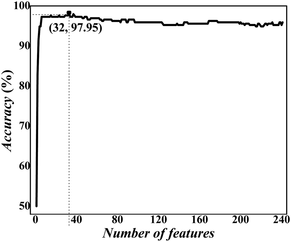
According to previous descriptions, to construct a robust and credible model, it is necessary to screen out key features from the 240 feature vectors. The mRMR method was used to rank the features. By adding the ranked features one by one according to the evaluations from mRMR, we established 240 SVM-based predictors. We then tested the prediction performance for the predictors and plotted the incremental feature selection curve as shown in Figure 2. When the top ranked 32 features were used, the maximum overall accuracy in the fivefold cross-validation test reached 97.95%. We also investigated the model's performance using jackknife cross-validation. Results showed that the overall accuracy of 97.62% was obtained, which was almost as high as that in fivefold cross-validated results. Interestingly, the 32 optimal features are all chemical properties, indicating that chemical properties play an important role in the prediction of 2′-O-methylation sites, whereas the nucleotide composition and type 2 PseKNC exist as noise. The principle of mRMR is to investigate whether there is correlation redundancy between features. Thus, we may conclude that sequence information and PseKNC cannot provide extra information to chemical properties for prediction. The chemical features are sufficient to describe the prediction problem of 2′-O-methylation sites.

OPEN IN VIEWER

FIG. 2.

A plot showing the incremental feature selection (IFS) procedure for identifying 2′-O-methylation site. When the top 32 features were used to perform prediction, the overall success rate reaches an IFS peak of 97.95% in fivefold cross-validation. IFS.

The detailed predictive performance of the predictors constructed from these 32 optimal features is expressed as follows: \documentclass{aastex}\usepackage{amsbsy}\usepackage{amsfonts}\usepackage{amssymb}\usepackage{bm}\usepackage{mathrsfs}\usepackage{pifont}\usepackage{stmaryrd}\usepackage{textcomp}\usepackage{portland, xspace}\usepackage{amsmath, amsxtra}\usepackage{upgreek}\pagestyle{empty}\DeclareMathSizes{10}{9}{7}{6}\begin{document} \begin{align*} \left\{ { \begin{matrix} {Sn = 97.27 \% \; \;} \\ {Sp = 98.63 \% \; \;} \\ {Acc = 97.95 \% } \\ {MCC = 0.959 \; \;} \\ \end{matrix} } \right.. \tag{18} \end{align*} \end{document}

We also drew the ROC curve as shown in Figure 3. The AUC reached 0.9955, indicating that the proposed method was a promising high-throughput tool for predicting 2′-O-methylation sites. Then, we compared it with the previous method (Chen et al., 2016b) and found that the feature screening could dramatically improve the accuracy (Table 3).

OPEN IN VIEWER

FIG. 3.

The receiver operating characteristic curve for identifying 2′-O-methylation sites.

In the process of modeling, a suitable classification method is important for fast and reliable model construction. Neural network has been widely used in pattern recognition, especially for deep learning (Cao et al., 2016, 2017a,b). However, deep learning is more suitable for high-dimensional and large-sized samples. Moreover, it consumes more time and computational resources for optimizing model parameters. However, SVM is suitable for modeling small samples. Furthermore, the accuracy of SVM is high enough.

In SVM, four kernel functions (linear kernel, polynomial kernel, RBF kernel, and sigmoid kernel) have been used in classification. RBF kernel function has been widely used in biological data classification because it can map a sample into a higher dimensional space. However, it is necessary to investigate the performances of different kernel functions for comparison. Table 4 gives the prediction results of four kernel functions. Four kernel functions produced high prediction accuracies (>95%), demonstrating that the optimized features could reflect the intrinsic characteristics of 2′-O-methylation. Among the four kernel functions, RBF produced the maximum accuracy. Thus, the final model was established based on the RBF kernel function.

3.4. Feature analysis

The mentioned results showed that our model could produce high accuracy. However, we also noticed that eight samples were not correctly predicted. Thus, we should further investigate why these samples were not correctly identified. At first, we statistically analyzed the distribution difference of the 32 optimal features between positive and negative samples with Equation (19). \documentclass{aastex}\usepackage{amsbsy}\usepackage{amsfonts}\usepackage{amssymb}\usepackage{bm}\usepackage{mathrsfs}\usepackage{pifont}\usepackage{stmaryrd}\usepackage{textcomp}\usepackage{portland, xspace}\usepackage{amsmath, amsxtra}\usepackage{upgreek}\pagestyle{empty}\DeclareMathSizes{10}{9}{7}{6}\begin{document} \begin{align*} { u_i } = \frac { { f_i^P - f_i^N } } { S } , \tag { 19 } \end{align*} \end{document}

where \documentclass{aastex}\usepackage{amsbsy}\usepackage{amsfonts}\usepackage{amssymb}\usepackage{bm}\usepackage{mathrsfs}\usepackage{pifont}\usepackage{stmaryrd}\usepackage{textcomp}\usepackage{portland, xspace}\usepackage{amsmath, amsxtra}\usepackage{upgreek}\pagestyle{empty}\DeclareMathSizes{10}{9}{7}{6}\begin{document} $$f_i^P$$ \end{document} and \documentclass{aastex}\usepackage{amsbsy}\usepackage{amsfonts}\usepackage{amssymb}\usepackage{bm}\usepackage{mathrsfs}\usepackage{pifont}\usepackage{stmaryrd}\usepackage{textcomp}\usepackage{portland, xspace}\usepackage{amsmath, amsxtra}\usepackage{upgreek}\pagestyle{empty}\DeclareMathSizes{10}{9}{7}{6}\begin{document} $$f_i^N$$ \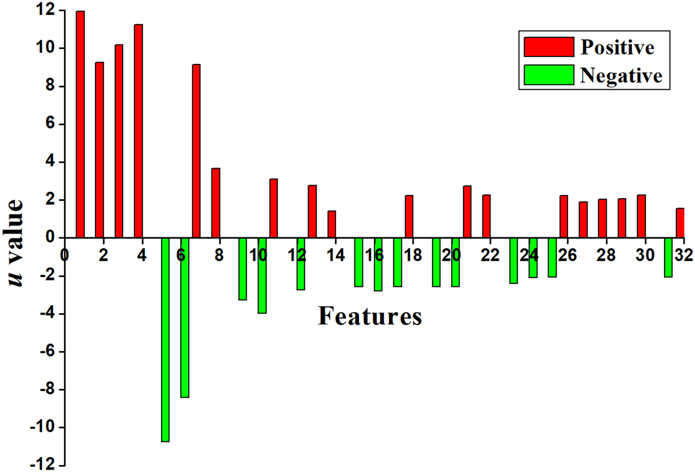end{document} , respectively, denote the occurrence frequencies of the i-th feature (i = 1, 2, …, 32) in positive and negative samples. The denominator S is a standard error. The 32 u values from 32 optimal features are plotted in Figure 4. Red (green) bars indicate that the features prefer to occur in positive (negative) samples.

OPEN IN VIEWER

FIG. 4.

A chromaticity diagram for the 32 optimal features. The red bars indicate that the features prefer positive samples, whereas green bars indicate the features prefer negative samples.

The eight incorrectly predicted samples including six incorrectly positive samples and two incorrectly negative samples. Further statistical results showed that the features of the six negative samples always occurred in positive samples. For example, all of them contain first four features (red) and excluded the fifth and sixth features. The two positive samples possessed the features that usually occurred in negative samples. Therefore, the eight samples were incorrectly predicted.

3.5. Web server guide

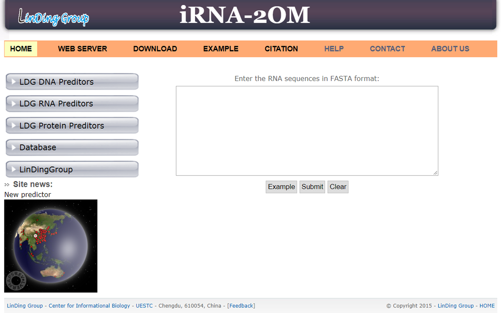
A web server can provide convenience for experimental scholars (Liang et al., 2017; Zhang et al., 2017). Thus, a novel platform obtained through the mentioned procedures has been developed and named “iRNA-2OM,” in which “i” means identify, “RNA” means the samples of RNA sequences, and “2OM” means 2′-O-methylation. A step-by-step guide of the web server is given as follows:

Step 1. Open the HOME at http://lin-group.cn/server/iRNA-2OM/ and you will see a brief introduction about the predictor.

OPEN IN VIEWER

FIG. 5.

A semiscreenshot for the WEBSERVER page of the iRNA-2OM web server at (http://lin-group.cn/server/iRNA-2OM).