With the rapid development of high-throughput genotyping and neuroimaging techniques, imaging genetics has drawn significant attention in the study of complex brain diseases such as Alzheimer's disease (AD). Research on the associations between genotype and phenotype improves the understanding of the genetic basis and biological mechanisms of brain structure and function. AD is a progressive neurodegenerative disease; therefore, the study on the relationship between single nucleotide polymorphism (SNP) and longitudinal variations of neuroimaging phenotype is crucial. Although some machine learning models have recently been proposed to capture longitudinal patterns in genotype–phenotype association studies, most machine-learning models base the learning on fixed structure among longitudinal prediction tasks rather than automatically learning the interrelationships. In response to this challenge, we propose a new automated time structure learning model to automatically reveal the longitudinal genotype–phenotype interactions and exploits such learned structure to enhance the phenotypic predictions. We proposed an efficient optimization algorithm for our model and provided rigorous theoretical convergence proof. We performed experiments on the Alzheimer's Disease Neuroimaging Initiative (ADNI) cohort for longitudinal phenotype prediction, including 3123 SNPs and 2 biomarkers (Voxel-Based Morphometry and FreeSurfer). The empirical results validate that our proposed model is superior to the counterparts. In addition, the best SNPs identified by our model have been replicated in the literature, which justifies our prediction.
1. Introduction
Alzheimer's Disease (AD) is the most prevalent and severe type of neurodegenerative disorder, which strongly affects human's memory, thinking, and behavior (Khachaturian, 1985). This disease is characterized by progressive memory impairment and other cognitive disabilities triggered by neuronal damage (Burns and Iliffe, 2009). AD usually progresses continuously, initially starting from the preclinical stage, then into mild cognitive impairment (MCI) and eventually into AD (Wenk, 2003). According to Alzheimer's Association (2016), AD is the sixth leading cause of death in the United States. Every 66 seconds, one person in the United States is developing AD. Until 2016, an estimate of 5.4 million people is living with AD in the United States, compared with 44 million worldwide. Worse, the world will see even more dramatic growth in these numbers in the short term if no breakthroughs are found.
With these facts, AD is gaining growing attention in this day and age. The current consensus emphasizes the need to understand the genetic causes of AD to prevent or slow down the progression in worsening the disease (Petrella et al., 2003). Recent advances in neuroimaging and microbiology have improved understanding of the links between genes, brain structure, and behavior (Hariri et al., 2006). At the same time, the rapid development of high-throughput genotyping enables the simultaneous measurement of hundreds of thousands or even millions of single nucleotide polymorphisms (SNPs) (Potkin et al., 2009a). These progresses have facilitated the pullulation of imaging genetics, which holds great promise for better understanding complex neurobiological systems.
In imaging genetics, an emerging strategy to facilitate the identification of susceptible disease-related genes is to use outcome-related biomarkers as quantitative traits (QTs) for genetic variation evaluation. Correlation studies between genetic variations and imaging studies often have significant advantages over case–control studies due to the following reason: QT is a quantitative measure with four to eight times more statistical power and significantly reduces the required sample size (Potkin et al., 2009b). A number of works have been reported to identify genetic factors affecting imaging phenotypes of biomedical importance (Harold et al., 2009; Shen et al., 2010; Bis et al., 2012).
In the genotype–phenotype association study, we can denote our inputs in the matrix format as follows: the SNP matrix \documentclass{aastex}\usepackage{amsbsy}\usepackage{amsfonts}\usepackage{amssymb}\usepackage{bm}\usepackage{mathrsfs}\usepackage{pifont}\usepackage{stmaryrd}\usepackage{textcomp}\usepackage{portland, xspace}\usepackage{amsmath, amsxtra}\usepackage{upgreek}\pagestyle{empty}\DeclareMathSizes{10}{9}{7}{6}\begin{document}
$$X \in { \mathbb{R}^{d \times n}}$$
\end{document} (n is the number or samples, d is the number of SNPs) and the imaging phenotype matrices \documentclass{aastex}\usepackage{amsbsy}\usepackage{amsfonts}\usepackage{amssymb}\usepackage{bm}\usepackage{mathrsfs}\usepackage{pifont}\usepackage{stmaryrd}\usepackage{textcomp}\usepackage{portland, xspace}\usepackage{amsmath, amsxtra}\usepackage{upgreek}\pagestyle{empty}\DeclareMathSizes{10}{9}{7}{6}\begin{document}
$$Y = [ {Y_1} , {Y_2} , \ldots , {Y_T} ] \in { \mathbb{R}^{n \times cT}}$$
\end{document} (c is the number of QTs, T is the number of time points, and \documentclass{aastex}\usepackage{amsbsy}\usepackage{amsfonts}\usepackage{amssymb}\usepackage{bm}\usepackage{mathrsfs}\usepackage{pifont}\usepackage{stmaryrd}\usepackage{textcomp}\usepackage{portland, xspace}\usepackage{amsmath, amsxtra}\usepackage{upgreek}\pagestyle{empty}\DeclareMathSizes{10}{9}{7}{6}\begin{document}
$${Y_t} \in { \mathbb{R}^{n \times c}}$$
\end{document} is the phenotype matrix at time t). The goal is to find the weight matrix \documentclass{aastex}\usepackage{amsbsy}\usepackage{amsfonts}\usepackage{amssymb}\usepackage{bm}\usepackage{mathrsfs}\usepackage{pifont}\usepackage{stmaryrd}\usepackage{textcomp}\usepackage{portland, xspace}\usepackage{amsmath, amsxtra}\usepackage{upgreek}\pagestyle{empty}\DeclareMathSizes{10}{9}{7}{6}\begin{document}
$$W = [ {W_1} , {W_2} , \ldots , {W_T} ] \in { \mathbb{R}^{d \times cT}}$$
\end{document}, which properly reflect the relations between SNPs and QTs and capture a subset of SNPs responsible for phenotype prediction at the same time. If we treat the prediction of one phenotype at one time point as a task, then the association study between genotypes with multiple longitudinal phenotypes can be seen as a multitask learning problem.
Conventional strategies (Ashford and Schmitt, 2001; Sabatti et al., 2008; Kim et al., 2009), which perform standard regression at all time points, are equivalent to carrying out regression at individual time point separately, thus ignore the longitudinal variations in brain phenotypes. Because AD is a progressive disorder, the imaging phenotype is a quantitative reflection of its neurodegenerative status, and predictive tasks at different points in time are reasonably assumed to be related. For a certain QT, its value at different times may be related, and different QTs at a certain time may also maintain a certain mutual influence. To explore the correlation between longitudinal prediction tasks, several multitasking models have been proposed based on sparse learning (Wang et al., 2012a,b). The main idea of these models is to apply the low-rank constraint to the entire parameter matrix such that the common subspace globally shared by different forecasting tasks can be extracted.
However, longitudinal forecasting tasks are interrelated rather than holistic. Existing methods cannot learn the correct relationship between tasks. Finding such a task group structure is tricky. The straightforward idea is to conduct clustering analysis on the prediction tasks and extract the group structure as a preprocessing step. However, such heuristic steps are not related to the overall longitudinal learning model, so the detected group structure is not optimal for longitudinal study. To bridge this gap, we propose a novel self-learned low-rank structured multitask learning model to simultaneously uncover the interrelations among different imaging phenotype predictions at different time points and utilize such interrelated structures to enhance the prediction tasks. We utilize the Schatten p-norm to identify the shared low-rank common subspace and impose the structure sparsity constraint through \documentclass{aastex}\usepackage{amsbsy}\usepackage{amsfonts}\usepackage{amssymb}\usepackage{bm}\usepackage{mathrsfs}\usepackage{pifont}\usepackage{stmaryrd}\usepackage{textcomp}\usepackage{portland, xspace}\usepackage{amsmath, amsxtra}\usepackage{upgreek}\pagestyle{empty}\DeclareMathSizes{10}{9}{7}{6}\begin{document}
$${ \ell _{2 , 0 + }}$$
\end{document}-norm. The new optimization algorithm is derived for the proposed objective. Our new model is applied to the Alzheimer's Disease Neuroimaging Initiative (ADNI) cohort for imaging phenotype prediction. All empirical results show that the proposed longitudinal feature learning model can more accurately predict phenotypes than related approaches.
Notations: In this article, matrices are all written as uppercase letters whereas vectors as bold lower case letters. For a matrix \documentclass{aastex}\usepackage{amsbsy}\usepackage{amsfonts}\usepackage{amssymb}\usepackage{bm}\usepackage{mathrsfs}\usepackage{pifont}\usepackage{stmaryrd}\usepackage{textcomp}\usepackage{portland, xspace}\usepackage{amsmath, amsxtra}\usepackage{upgreek}\pagestyle{empty}\DeclareMathSizes{10}{9}{7}{6}\begin{document}
$$M \in { \mathbb{R}^{d \times n}}$$
\end{document}, its i-th row and j-th column are denoted by \documentclass{aastex}\usepackage{amsbsy}\usepackage{amsfonts}\usepackage{amssymb}\usepackage{bm}\usepackage{mathrsfs}\usepackage{pifont}\usepackage{stmaryrd}\usepackage{textcomp}\usepackage{portland, xspace}\usepackage{amsmath, amsxtra}\usepackage{upgreek}\pagestyle{empty}\DeclareMathSizes{10}{9}{7}{6}\begin{document}
$${{ \bf m}^i}$$
\end{document}, \documentclass{aastex}\usepackage{amsbsy}\usepackage{amsfonts}\usepackage{amssymb}\usepackage{bm}\usepackage{mathrsfs}\usepackage{pifont}\usepackage{stmaryrd}\usepackage{textcomp}\usepackage{portland, xspace}\usepackage{amsmath, amsxtra}\usepackage{upgreek}\pagestyle{empty}\DeclareMathSizes{10}{9}{7}{6}\begin{document}
$${{ \bf m}_j}$$
\end{document}, respectively, whereas its ij-th element is written as \documentclass{aastex}\usepackage{amsbsy}\usepackage{amsfonts}\usepackage{amssymb}\usepackage{bm}\usepackage{mathrsfs}\usepackage{pifont}\usepackage{stmaryrd}\usepackage{textcomp}\usepackage{portland, xspace}\usepackage{amsmath, amsxtra}\usepackage{upgreek}\pagestyle{empty}\DeclareMathSizes{10}{9}{7}{6}\begin{document}
$${m_{ij}}$$
\end{document} or M(i,j) For a positive value p, the \documentclass{aastex}\usepackage{amsbsy}\usepackage{amsfonts}\usepackage{amssymb}\usepackage{bm}\usepackage{mathrsfs}\usepackage{pifont}\usepackage{stmaryrd}\usepackage{textcomp}\usepackage{portland, xspace}\usepackage{amsmath, amsxtra}\usepackage{upgreek}\pagestyle{empty}\DeclareMathSizes{10}{9}{7}{6}\begin{document}
$${ \ell _{2 , p}}$$
\end{document}-norm of M is defined as \documentclass{aastex}\usepackage{amsbsy}\usepackage{amsfonts}\usepackage{amssymb}\usepackage{bm}\usepackage{mathrsfs}\usepackage{pifont}\usepackage{stmaryrd}\usepackage{textcomp}\usepackage{portland, xspace}\usepackage{amsmath, amsxtra}\usepackage{upgreek}\pagestyle{empty}\DeclareMathSizes{10}{9}{7}{6}\begin{document}
$$ { \parallel M \parallel_ { 2 , p } } = { \left( { \mathop { \sum } \nolimits_ { i = 1 } ^d { { \left( { \mathop { \sum } \nolimits_ { j = 1 } ^n \;m_ { ij } ^2 } \right) } ^ { \frac { p } { 2 } } } } \right) ^ { \frac { 1 } { p } } } = { \left( { \mathop { \sum } \nolimits_ { i = 1 } ^d { { \left( { { { \parallel { { { \bf m } ^i } } \parallel } _2 } } \right) } ^p } } \right) ^ { \frac { 1 } { p } } } $$
\end{document}.
2. Temporal Structure Auto-Learning Predictive Model
2.1. Illustration of our idea
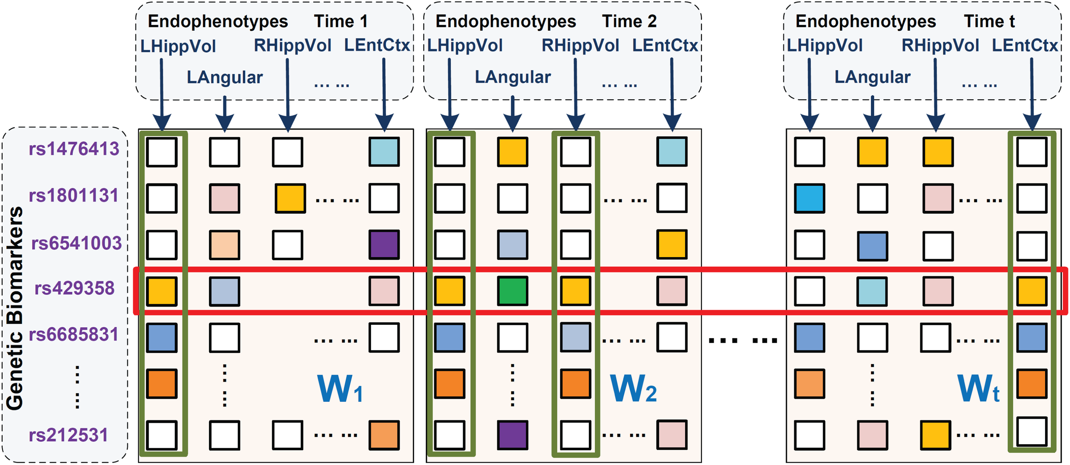
Our main purpose is to construct a model to simultaneously detect the latent group structure of longitudinal phenotype prediction tasks and study SNP associations across all endophenotypes. As is shown in Figure 1, the four phenotypes marked by the green rectangles have similar distributions and are very likely to be correlated. However, previous models are not capable of capturing such interlinked structures in different task groups. In our model, we expect to uncover such latent subspaces in different groups through low-rank constraints. Meanwhile, the SNP loci marked by the red rectangle, rs429358, appear to be predominant for most response variables. Correspondingly, we impose a sparsity constraint to pick it out. In consequence, our model should be able to capture the group structure within the prediction tasks and utilize this information to select prominent SNPs across the relevant phenotypes. In the next subsection, we will elaborate how to translate these ideas into the new learning model.
Illustration of our temporal structure auto-learning regression model. In this figure, parameter matrices at different time points are arranged in the column order. Four tasks marked out by green rectangles obey similar patterns thus have high interrelations while one SNP loci rs429358 enclosed by a red rectangle appears to be correlated with most phenotypes. Our model is meant to uncover the group information among all prediction tasks along the time continuum, that is, cluster the phenotypes in the same latent subspace (phenotypes marked out by green rectangles) into the same group and meanwhile discover genetic biomarkers responsible for most prediction tasks (SNPs marked out by red rectangles). SNPs, single nucleotide polymorphisms.
2.2. New objective function
To discover the group structure of phenotype prediction tasks, we introduce and optimize a group index matrix set Q. Suppose the tasks come from g groups, then we have \documentclass{aastex}\usepackage{amsbsy}\usepackage{amsfonts}\usepackage{amssymb}\usepackage{bm}\usepackage{mathrsfs}\usepackage{pifont}\usepackage{stmaryrd}\usepackage{textcomp}\usepackage{portland, xspace}\usepackage{amsmath, amsxtra}\usepackage{upgreek}\pagestyle{empty}\DeclareMathSizes{10}{9}{7}{6}\begin{document}
$$Q = \{ {Q_1} , {Q_2} , \ldots , {Q_g} \} $$
\end{document}, where Qi is a diagonal matrix and \documentclass{aastex}\usepackage{amsbsy}\usepackage{amsfonts}\usepackage{amssymb}\usepackage{bm}\usepackage{mathrsfs}\usepackage{pifont}\usepackage{stmaryrd}\usepackage{textcomp}\usepackage{portland, xspace}\usepackage{amsmath, amsxtra}\usepackage{upgreek}\pagestyle{empty}\DeclareMathSizes{10}{9}{7}{6}\begin{document}
$${Q_i} \in { \{ 0 , 1 \} ^{cT \times cT}}$$
\end{document}. For each Qi, \documentclass{aastex}\usepackage{amsbsy}\usepackage{amsfonts}\usepackage{amssymb}\usepackage{bm}\usepackage{mathrsfs}\usepackage{pifont}\usepackage{stmaryrd}\usepackage{textcomp}\usepackage{portland, xspace}\usepackage{amsmath, amsxtra}\usepackage{upgreek}\pagestyle{empty}\DeclareMathSizes{10}{9}{7}{6}\begin{document}
$${ ( {Q_i} ) _{ ( k , k ) }} = 1$$
\end{document} means the k-th feature belongs to the i-th group, whereas \documentclass{aastex}\usepackage{amsbsy}\usepackage{amsfonts}\usepackage{amssymb}\usepackage{bm}\usepackage{mathrsfs}\usepackage{pifont}\usepackage{stmaryrd}\usepackage{textcomp}\usepackage{portland, xspace}\usepackage{amsmath, amsxtra}\usepackage{upgreek}\pagestyle{empty}\DeclareMathSizes{10}{9}{7}{6}\begin{document}
$${ ( {Q_i} ) _{ ( k , k ) }} = 0$$
\end{document} means not. To avoid overlap of subspaces, we maintain the constraint that \documentclass{aastex}\usepackage{amsbsy}\usepackage{amsfonts}\usepackage{amssymb}\usepackage{bm}\usepackage{mathrsfs}\usepackage{pifont}\usepackage{stmaryrd}\usepackage{textcomp}\usepackage{portland, xspace}\usepackage{amsmath, amsxtra}\usepackage{upgreek}\pagestyle{empty}\DeclareMathSizes{10}{9}{7}{6}\begin{document}
$$\sum \nolimits_{i = 1}^g \;{Q_i} = I$$
\end{document}.
On the other hand, since SNPs are often correlated and have an overlap in impacting phenotypes, we impose low-rank constraint to uncover the common subspaces shared by prediction tasks. The traditional method to impose low-rank constraint is minimizing trace norm, which is a convex relaxation of rank minimization problem. However, trace norm is not an ideal approximation of the rank minimization. In this study, we use the Schatten p-norm regularization term instead, which approximates the rank minimization better than trace norm (Nie et al., 2012). The definition of Schatten p-norm of a matrix \documentclass{aastex}\usepackage{amsbsy}\usepackage{amsfonts}\usepackage{amssymb}\usepackage{bm}\usepackage{mathrsfs}\usepackage{pifont}\usepackage{stmaryrd}\usepackage{textcomp}\usepackage{portland, xspace}\usepackage{amsmath, amsxtra}\usepackage{upgreek}\pagestyle{empty}\DeclareMathSizes{10}{9}{7}{6}\begin{document}
$$M \in { \mathbb{R}^{m \times n}}$$
\end{document} is:
\documentclass{aastex}\usepackage{amsbsy}\usepackage{amsfonts}\usepackage{amssymb}\usepackage{bm}\usepackage{mathrsfs}\usepackage{pifont}\usepackage{stmaryrd}\usepackage{textcomp}\usepackage{portland, xspace}\usepackage{amsmath, amsxtra}\usepackage{upgreek}\pagestyle{empty}\DeclareMathSizes{10}{9}{7}{6}\begin{document}
\begin{align*}
{ \parallel M \parallel_ { { S_p } } } = ( Tr ( ( { M^T } M { ) ^ { \frac { p } { 2 } } } { ) ) ^ { \frac { 1 } { p } } } = \left( \mathop \sum \limits_ { i = 1 } ^ { \min \ { m , n \ } } \sigma _i^p \right) { ^ { \frac { 1 } { p } } } { \kern 1pt } , \tag { 1 }
\end{align*}
\end{document}
where \documentclass{aastex}\usepackage{amsbsy}\usepackage{amsfonts}\usepackage{amssymb}\usepackage{bm}\usepackage{mathrsfs}\usepackage{pifont}\usepackage{stmaryrd}\usepackage{textcomp}\usepackage{portland, xspace}\usepackage{amsmath, amsxtra}\usepackage{upgreek}\pagestyle{empty}\DeclareMathSizes{10}{9}{7}{6}\begin{document}
$${ \sigma _i}$$
\end{document} is the i-th singular value of M. Specially, when p = 1, the Schatten p-norm of M is exactly the trace norm since
\documentclass{aastex}\usepackage{amsbsy}\usepackage{amsfonts}\usepackage{amssymb}\usepackage{bm}\usepackage{mathrsfs}\usepackage{pifont}\usepackage{stmaryrd}\usepackage{textcomp}\usepackage{portland, xspace}\usepackage{amsmath, amsxtra}\usepackage{upgreek}\pagestyle{empty}\DeclareMathSizes{10}{9}{7}{6}\begin{document}
\begin{align*}
{ \parallel M \parallel _* } = { \parallel M \parallel _ { { S_1 } } } = Tr ( ( { M^T } M { ) ^ { \frac { 1 } { 2 } } } ) = \mathop \sum \limits_ { i = 1 } ^ { \min \ { m , n \ } } { \sigma _i } { \kern 1pt } . \tag { 2 }
\end{align*}
\end{document}
As we recall, the rank of M can be denoted as \documentclass{aastex}\usepackage{amsbsy}\usepackage{amsfonts}\usepackage{amssymb}\usepackage{bm}\usepackage{mathrsfs}\usepackage{pifont}\usepackage{stmaryrd}\usepackage{textcomp}\usepackage{portland, xspace}\usepackage{amsmath, amsxtra}\usepackage{upgreek}\pagestyle{empty}\DeclareMathSizes{10}{9}{7}{6}\begin{document}
$${ \rm{rank}} ( M ) = \sum \nolimits_{i = 1}^{ \min \{ m , n \} } \sigma _i^0$$
\end{document}, where \documentclass{aastex}\usepackage{amsbsy}\usepackage{amsfonts}\usepackage{amssymb}\usepackage{bm}\usepackage{mathrsfs}\usepackage{pifont}\usepackage{stmaryrd}\usepackage{textcomp}\usepackage{portland, xspace}\usepackage{amsmath, amsxtra}\usepackage{upgreek}\pagestyle{empty}\DeclareMathSizes{10}{9}{7}{6}\begin{document}
$${0^0} = 0$$
\end{document}. Thus, when \documentclass{aastex}\usepackage{amsbsy}\usepackage{amsfonts}\usepackage{amssymb}\usepackage{bm}\usepackage{mathrsfs}\usepackage{pifont}\usepackage{stmaryrd}\usepackage{textcomp}\usepackage{portland, xspace}\usepackage{amsmath, amsxtra}\usepackage{upgreek}\pagestyle{empty}\DeclareMathSizes{10}{9}{7}{6}\begin{document}
$$0 < p < 1$$
\end{document}, Schatten p-norm is a better low-rank regularization than trace norm.
Moreover, since we intend to integrate the SNP selection procedure across multiple learning tasks, here we impose a sparsity constraint. One possible approach is \documentclass{aastex}\usepackage{amsbsy}\usepackage{amsfonts}\usepackage{amssymb}\usepackage{bm}\usepackage{mathrsfs}\usepackage{pifont}\usepackage{stmaryrd}\usepackage{textcomp}\usepackage{portland, xspace}\usepackage{amsmath, amsxtra}\usepackage{upgreek}\pagestyle{empty}\DeclareMathSizes{10}{9}{7}{6}\begin{document}
$${ \ell _{2 , 1}}$$
\end{document}-norm regularization (Obozinski et al., 2006), which is popularly utilized owing to its convex property. However, the real data usually do not satisfy the restricted isometry property (RIP), thus the solution of \documentclass{aastex}\usepackage{amsbsy}\usepackage{amsfonts}\usepackage{amssymb}\usepackage{bm}\usepackage{mathrsfs}\usepackage{pifont}\usepackage{stmaryrd}\usepackage{textcomp}\usepackage{portland, xspace}\usepackage{amsmath, amsxtra}\usepackage{upgreek}\pagestyle{empty}\DeclareMathSizes{10}{9}{7}{6}\begin{document}
$${ \ell _{2 , 1}}$$
\end{document}-norm may not be sparse enough. See (Candès, 2008; Cai and Zhang, 2013) for details. To solve this problem, in our model, we resort to a stricter sparsity constraint, \documentclass{aastex}\usepackage{amsbsy}\usepackage{amsfonts}\usepackage{amssymb}\usepackage{bm}\usepackage{mathrsfs}\usepackage{pifont}\usepackage{stmaryrd}\usepackage{textcomp}\usepackage{portland, xspace}\usepackage{amsmath, amsxtra}\usepackage{upgreek}\pagestyle{empty}\DeclareMathSizes{10}{9}{7}{6}\begin{document}
$${ \ell _{2 , 0 + }}$$
\end{document}-norm, which is defined as follows:
\documentclass{aastex}\usepackage{amsbsy}\usepackage{amsfonts}\usepackage{amssymb}\usepackage{bm}\usepackage{mathrsfs}\usepackage{pifont}\usepackage{stmaryrd}\usepackage{textcomp}\usepackage{portland, xspace}\usepackage{amsmath, amsxtra}\usepackage{upgreek}\pagestyle{empty}\DeclareMathSizes{10}{9}{7}{6}\begin{document}
\begin{align*}
{\parallel M \parallel _{2 , q}} = \left( \mathop { \sum } \limits_{i = 1}^d { \left( \mathop { \sum } \limits_{j = 1}^n m_{ij}^2 \right) ^{{q \over 2}}} \right) ^{{1 \over q}} = \left( \mathop \sum\limits_{i = 1}^d { ( { \parallel {{{\bf m}^i}} \parallel_2})^q}\right)^{{1 \over q}} ,
\end{align*}
\end{document}
where q is a positive value. Similarly to the previous discussion, when \documentclass{aastex}\usepackage{amsbsy}\usepackage{amsfonts}\usepackage{amssymb}\usepackage{bm}\usepackage{mathrsfs}\usepackage{pifont}\usepackage{stmaryrd}\usepackage{textcomp}\usepackage{portland, xspace}\usepackage{amsmath, amsxtra}\usepackage{upgreek}\pagestyle{empty}\DeclareMathSizes{10}{9}{7}{6}\begin{document}
$$0 < q < 1$$
\end{document}, \documentclass{aastex}\usepackage{amsbsy}\usepackage{amsfonts}\usepackage{amssymb}\usepackage{bm}\usepackage{mathrsfs}\usepackage{pifont}\usepackage{stmaryrd}\usepackage{textcomp}\usepackage{portland, xspace}\usepackage{amsmath, amsxtra}\usepackage{upgreek}\pagestyle{empty}\DeclareMathSizes{10}{9}{7}{6}\begin{document}
$${ \ell _{2 , 0 + }}$$
\end{document}-norm can achieve a more sparse solution than \documentclass{aastex}\usepackage{amsbsy}\usepackage{amsfonts}\usepackage{amssymb}\usepackage{bm}\usepackage{mathrsfs}\usepackage{pifont}\usepackage{stmaryrd}\usepackage{textcomp}\usepackage{portland, xspace}\usepackage{amsmath, amsxtra}\usepackage{upgreek}\pagestyle{empty}\DeclareMathSizes{10}{9}{7}{6}\begin{document}
$${ \ell _{2 , 1}}$$
\end{document} norm.
In Equation (3), we adopt the k-power of Schatten p-norm to make our model more robust. The use of parameter k will be articulated in Section 4. Since it is difficult to solve the proposed new nonconvex and nonsmooth objective, in the next section we propose a novel alternating optimization method for Problem (3).
3. Optimization Algorithm
In this section, we first introduce an optimization algorithm for general problems with Problem (3) being a special case, and then discuss the detailed optimization steps of Problem (3).
Lemma 1Let\documentclass{aastex}\usepackage{amsbsy}\usepackage{amsfonts}\usepackage{amssymb}\usepackage{bm}\usepackage{mathrsfs}\usepackage{pifont}\usepackage{stmaryrd}\usepackage{textcomp}\usepackage{portland, xspace}\usepackage{amsmath, amsxtra}\usepackage{upgreek}\pagestyle{empty}\DeclareMathSizes{10}{9}{7}{6}\begin{document}
$${g_i} ( x )$$
\end{document}denote a general function over x, where x can be a scalar, vector or matrix, then we can claim:
When\documentclass{aastex}\usepackage{amsbsy}\usepackage{amsfonts}\usepackage{amssymb}\usepackage{bm}\usepackage{mathrsfs}\usepackage{pifont}\usepackage{stmaryrd}\usepackage{textcomp}\usepackage{portland, xspace}\usepackage{amsmath, amsxtra}\usepackage{upgreek}\pagestyle{empty}\DeclareMathSizes{10}{9}{7}{6}\begin{document}
$$\delta \to 0$$
\end{document}, The optimization problem\documentclass{aastex}\usepackage{amsbsy}\usepackage{amsfonts}\usepackage{amssymb}\usepackage{bm}\usepackage{mathrsfs}\usepackage{pifont}\usepackage{stmaryrd}\usepackage{textcomp}\usepackage{portland, xspace}\usepackage{amsmath, amsxtra}\usepackage{upgreek}\pagestyle{empty}\DeclareMathSizes{10}{9}{7}{6}\begin{document}
\begin{align*}
\mathop { \min } \limits_ { x \in { \cal C } } f ( x ) + \mathop \sum \limits_i Tr ( ( g_i^T ( x ) { g_i } ( x { ) ) ^ { \frac { p } { 2 } } } )
\end{align*}
\end{document}
is equivalent to\documentclass{aastex}\usepackage{amsbsy}\usepackage{amsfonts}\usepackage{amssymb}\usepackage{bm}\usepackage{mathrsfs}\usepackage{pifont}\usepackage{stmaryrd}\usepackage{textcomp}\usepackage{portland, xspace}\usepackage{amsmath, amsxtra}\usepackage{upgreek}\pagestyle{empty}\DeclareMathSizes{10}{9}{7}{6}\begin{document}
\begin{align*}
\mathop { \min } \limits_ { x \in { \cal C } } f ( x ) + \mathop \sum \limits_i Tr ( g_i^T ( x ) { g_i } ( x ) { D_i } ) , \quad where \ { D_i } = \frac { p } { 2 } { ( g_i^T ( x ) { g_i } ( x ) + \delta I ) ^ { \frac { { p - 2 } } { 2 } } } { \kern 1pt } . \tag { 4 }
\end{align*}
\end{document}
Proof. When \documentclass{aastex}\usepackage{amsbsy}\usepackage{amsfonts}\usepackage{amssymb}\usepackage{bm}\usepackage{mathrsfs}\usepackage{pifont}\usepackage{stmaryrd}\usepackage{textcomp}\usepackage{portland, xspace}\usepackage{amsmath, amsxtra}\usepackage{upgreek}\pagestyle{empty}\DeclareMathSizes{10}{9}{7}{6}\begin{document}
$$\delta \to 0$$
\end{document}, it is apparent that the optimization problem
\documentclass{aastex}\usepackage{amsbsy}\usepackage{amsfonts}\usepackage{amssymb}\usepackage{bm}\usepackage{mathrsfs}\usepackage{pifont}\usepackage{stmaryrd}\usepackage{textcomp}\usepackage{portland, xspace}\usepackage{amsmath, amsxtra}\usepackage{upgreek}\pagestyle{empty}\DeclareMathSizes{10}{9}{7}{6}\begin{document}
\begin{align*}
\mathop { \min } \limits_ { x \in { \cal C } } f ( x ) + \mathop \sum \limits_i Tr ( ( g_i^T ( x ) { g_i } ( x ) + \delta I { ) ^ { \frac { p } { 2 } } } ) \tag { 5 }
\end{align*}
\end{document}
will reduce to
\documentclass{aastex}\usepackage{amsbsy}\usepackage{amsfonts}\usepackage{amssymb}\usepackage{bm}\usepackage{mathrsfs}\usepackage{pifont}\usepackage{stmaryrd}\usepackage{textcomp}\usepackage{portland, xspace}\usepackage{amsmath, amsxtra}\usepackage{upgreek}\pagestyle{empty}\DeclareMathSizes{10}{9}{7}{6}\begin{document}
\begin{align*}
\mathop { \min } \limits_ { x \in { \cal C } } f ( x ) + \mathop \sum \limits_i Tr ( ( g_i^T ( x ) { g_i } ( x { ) ) ^ { \frac { p } { 2 } } } ) { \kern 1pt } . \tag { 6 }
\end{align*}
\end{document}
So we turn the nonsmooth Problem (6) to the smooth Problem (5) where \documentclass{aastex}\usepackage{amsbsy}\usepackage{amsfonts}\usepackage{amssymb}\usepackage{bm}\usepackage{mathrsfs}\usepackage{pifont}\usepackage{stmaryrd}\usepackage{textcomp}\usepackage{portland, xspace}\usepackage{amsmath, amsxtra}\usepackage{upgreek}\pagestyle{empty}\DeclareMathSizes{10}{9}{7}{6}\begin{document}
$$\delta$$
\end{document} is fairly small.
The Lagrangian function of Problem (5) is:
\documentclass{aastex}\usepackage{amsbsy}\usepackage{amsfonts}\usepackage{amssymb}\usepackage{bm}\usepackage{mathrsfs}\usepackage{pifont}\usepackage{stmaryrd}\usepackage{textcomp}\usepackage{portland, xspace}\usepackage{amsmath, amsxtra}\usepackage{upgreek}\pagestyle{empty}\DeclareMathSizes{10}{9}{7}{6}\begin{document}
\begin{align*}
\mathcal { L } ( x , \lambda ) = f ( x ) + \mathop \sum \limits_i Tr ( ( g_i^T ( x ) { g_i } ( x ) + \delta I { ) ^ { \frac { p } { 2 } } } ) - r ( x , \lambda ) { \kern 1pt } , \tag { 7 }
\end{align*}
\end{document}
where \documentclass{aastex}\usepackage{amsbsy}\usepackage{amsfonts}\usepackage{amssymb}\usepackage{bm}\usepackage{mathrsfs}\usepackage{pifont}\usepackage{stmaryrd}\usepackage{textcomp}\usepackage{portland, xspace}\usepackage{amsmath, amsxtra}\usepackage{upgreek}\pagestyle{empty}\DeclareMathSizes{10}{9}{7}{6}\begin{document}
$$r ( x , \lambda )$$
\end{document} is a Lagrangian term for the domain constraint \documentclass{aastex}\usepackage{amsbsy}\usepackage{amsfonts}\usepackage{amssymb}\usepackage{bm}\usepackage{mathrsfs}\usepackage{pifont}\usepackage{stmaryrd}\usepackage{textcomp}\usepackage{portland, xspace}\usepackage{amsmath, amsxtra}\usepackage{upgreek}\pagestyle{empty}\DeclareMathSizes{10}{9}{7}{6}\begin{document}
$$x \in { \cal C}$$
\end{document}. Take derivative w.r.t. x and set it to 0, we have:
\documentclass{aastex}\usepackage{amsbsy}\usepackage{amsfonts}\usepackage{amssymb}\usepackage{bm}\usepackage{mathrsfs}\usepackage{pifont}\usepackage{stmaryrd}\usepackage{textcomp}\usepackage{portland, xspace}\usepackage{amsmath, amsxtra}\usepackage{upgreek}\pagestyle{empty}\DeclareMathSizes{10}{9}{7}{6}\begin{document}
\begin{align*}
f ^\prime ( x ) + \mathop \sum \limits_i { \frac { \partial Tr ( ( g_i^T ( x ) { g_i } ( x ) + \delta I { ) ^ { \frac { p } { 2 } } } ) } { \partial x } } - { \frac { \partial r ( x , \lambda ) } { \partial x } } = 0 { \kern 1pt } . \tag { 8 }
\end{align*}
\end{document}
Based on the chain rule (Bentler and Lee, 1978), Equation (8) can be rewritten as:
\documentclass{aastex}\usepackage{amsbsy}\usepackage{amsfonts}\usepackage{amssymb}\usepackage{bm}\usepackage{mathrsfs}\usepackage{pifont}\usepackage{stmaryrd}\usepackage{textcomp}\usepackage{portland, xspace}\usepackage{amsmath, amsxtra}\usepackage{upgreek}\pagestyle{empty}\DeclareMathSizes{10}{9}{7}{6}\begin{document}
\begin{align*}
f^\prime ( x ) + \mathop \sum \limits_i { \frac { tr \left( { 2 { p } { 2 } { { ( g_i^T ( x ) { g_i } ( x ) + \delta I ) } ^ {\frac { { p - 2 } } { 2 } } } g_i^T ( x ) \partial { g_i } ( x ) } \right) } {\partial x } } - { \frac { \partial r ( x , \lambda ) } {\partial x } } = 0 . \tag {9}
\end{align*}
\end{document}
According to the Karush–Kuhn–Tucker conditions (Rockafellar, 1970), if we can find a solution x that satisfies Equation (9), then we usually find a local/global optimal solution to Problem (5). However, it is intractable to directly find the solution x that satisfies Equation (9). Here we come up with a strategy as follows:
If we define \documentclass{aastex}\usepackage{amsbsy}\usepackage{amsfonts}\usepackage{amssymb}\usepackage{bm}\usepackage{mathrsfs}\usepackage{pifont}\usepackage{stmaryrd}\usepackage{textcomp}\usepackage{portland, xspace}\usepackage{amsmath, amsxtra}\usepackage{upgreek}\pagestyle{empty}\DeclareMathSizes{10}{9}{7}{6}\begin{document}
$$ { D_i } = \frac { p } { 2 } { ( g_i^T ( x ) { g_i } ( x ) + \delta I ) ^ { \frac { { p - 2 } } { 2 } } } $$
\end{document} as a given constant, then Equation (9) can be reduced to
\documentclass{aastex}\usepackage{amsbsy}\usepackage{amsfonts}\usepackage{amssymb}\usepackage{bm}\usepackage{mathrsfs}\usepackage{pifont}\usepackage{stmaryrd}\usepackage{textcomp}\usepackage{portland, xspace}\usepackage{amsmath, amsxtra}\usepackage{upgreek}\pagestyle{empty}\DeclareMathSizes{10}{9}{7}{6}\begin{document}
\begin{align*}
f ^\prime ( x ) + \mathop \sum \limits_i { \frac { tr \left( { 2 { D_i } g_i^T ( x ) \partial { g_i } ( x ) } \right) } { \partial x } } - { \frac { \partial r ( x , \lambda ) } { \partial x } } = 0 { \kern 1pt } . \tag { 10 }
\end{align*}
\end{document}
Based on the chain rule (Bentler and Lee, 1978), the optimal solution \documentclass{aastex}\usepackage{amsbsy}\usepackage{amsfonts}\usepackage{amssymb}\usepackage{bm}\usepackage{mathrsfs}\usepackage{pifont}\usepackage{stmaryrd}\usepackage{textcomp}\usepackage{portland, xspace}\usepackage{amsmath, amsxtra}\usepackage{upgreek}\pagestyle{empty}\DeclareMathSizes{10}{9}{7}{6}\begin{document}
$${x^*}$$
\end{document} of Equation (10) is also an optimal solution to the following problem:
\documentclass{aastex}\usepackage{amsbsy}\usepackage{amsfonts}\usepackage{amssymb}\usepackage{bm}\usepackage{mathrsfs}\usepackage{pifont}\usepackage{stmaryrd}\usepackage{textcomp}\usepackage{portland, xspace}\usepackage{amsmath, amsxtra}\usepackage{upgreek}\pagestyle{empty}\DeclareMathSizes{10}{9}{7}{6}\begin{document}
\begin{align*}
\mathop { \min } \limits_{x \in { \cal C}} f ( x ) + \mathop \sum \limits_i Tr ( g_i^T ( x ) {g_i} ( x ) {D_i} ) { \kern 1pt} . \tag{11}
\end{align*}
\end{document}
Based on this observation, we can first guess a solution x, next calculate Di based on the current solution x, and then update the current solution x by the optimal solution of Problem (11) on the basis of the calculated Di. We can iteratively perform this procedure until it converges. ▪
where Di is defined as:
\documentclass{aastex}\usepackage{amsbsy}\usepackage{amsfonts}\usepackage{amssymb}\usepackage{bm}\usepackage{mathrsfs}\usepackage{pifont}\usepackage{stmaryrd}\usepackage{textcomp}\usepackage{portland, xspace}\usepackage{amsmath, amsxtra}\usepackage{upgreek}\pagestyle{empty}\DeclareMathSizes{10}{9}{7}{6}\begin{document}
\begin{align*}
{ D_i } = \frac { { kp } } { 2 } { ( \parallel { W { Q_i } } \parallel_ { { S_p } } ^p ) ^ { k - 1 } } { ( W { Q_i } { W^T } + { \delta _1 } I ) ^ { \frac { { p - 2 } } { 2 } } } { \kern 1pt } , \tag { 13 }
\end{align*}
\end{document}
and B is defined as a diagonal matrix with the l-th diagonal element to be:
\documentclass{aastex}\usepackage{amsbsy}\usepackage{amsfonts}\usepackage{amssymb}\usepackage{bm}\usepackage{mathrsfs}\usepackage{pifont}\usepackage{stmaryrd}\usepackage{textcomp}\usepackage{portland, xspace}\usepackage{amsmath, amsxtra}\usepackage{upgreek}\pagestyle{empty}\DeclareMathSizes{10}{9}{7}{6}\begin{document}
\begin{align*}
{ b_ { ll } } = \frac { q } { 2 } { ( { { \bf { w } } ^l } { ( { { \bf { w } } ^l } ) ^T } + { \delta _2 } I ) ^ { \frac { { q - 2 } } { 2 } } } { \kern 1pt } , \tag { 14 }
\end{align*}
\end{document}
and \documentclass{aastex}\usepackage{amsbsy}\usepackage{amsfonts}\usepackage{amssymb}\usepackage{bm}\usepackage{mathrsfs}\usepackage{pifont}\usepackage{stmaryrd}\usepackage{textcomp}\usepackage{portland, xspace}\usepackage{amsmath, amsxtra}\usepackage{upgreek}\pagestyle{empty}\DeclareMathSizes{10}{9}{7}{6}\begin{document}
$${ \delta _1}$$
\end{document} and \documentclass{aastex}\usepackage{amsbsy}\usepackage{amsfonts}\usepackage{amssymb}\usepackage{bm}\usepackage{mathrsfs}\usepackage{pifont}\usepackage{stmaryrd}\usepackage{textcomp}\usepackage{portland, xspace}\usepackage{amsmath, amsxtra}\usepackage{upgreek}\pagestyle{empty}\DeclareMathSizes{10}{9}{7}{6}\begin{document}
$${ \delta _2}$$
\end{document} are two fairly small parameters close to 0.
We can solve Problem (12) through alternating optimization.
Let \documentclass{aastex}\usepackage{amsbsy}\usepackage{amsfonts}\usepackage{amssymb}\usepackage{bm}\usepackage{mathrsfs}\usepackage{pifont}\usepackage{stmaryrd}\usepackage{textcomp}\usepackage{portland, xspace}\usepackage{amsmath, amsxtra}\usepackage{upgreek}\pagestyle{empty}\DeclareMathSizes{10}{9}{7}{6}\begin{document}
$${A_i} = {W^T}{D_i}W$$
\end{document}, then the solution of each Qi is as follows:
\documentclass{aastex}\usepackage{amsbsy}\usepackage{amsfonts}\usepackage{amssymb}\usepackage{bm}\usepackage{mathrsfs}\usepackage{pifont}\usepackage{stmaryrd}\usepackage{textcomp}\usepackage{portland, xspace}\usepackage{amsmath, amsxtra}\usepackage{upgreek}\pagestyle{empty}\DeclareMathSizes{10}{9}{7}{6}\begin{document}
\begin{align*}
{Q_i} ( k , k ) = \left\{ \begin{matrix} 1 , \quad \quad \quad i = {\rm arg} \mathop { \min } \limits_j \,{A_j} ( k , \,k ) \hfill \\ 0 , \quad \quad \quad \quad \; \;{ \rm{otherwise}} \hfill \\\end{matrix} \right. \tag{15}
\end{align*}
\end{document}
The second step is fixing Q and solving W. Problem (12) becomes:
\documentclass{aastex}\usepackage{amsbsy}\usepackage{amsfonts}\usepackage{amssymb}\usepackage{bm}\usepackage{mathrsfs}\usepackage{pifont}\usepackage{stmaryrd}\usepackage{textcomp}\usepackage{portland, xspace}\usepackage{amsmath, amsxtra}\usepackage{upgreek}\pagestyle{empty}\DeclareMathSizes{10}{9}{7}{6}\begin{document}
\begin{align*}
\mathop { \min } \limits_W \parallel {{X^T}W - Y} \parallel_F^2 + { \gamma _1}{ \kern 1pt} \mathop \sum \limits_{i = 1}^g { \kern 1pt} Tr ( W{Q_i}{W^T}{D_i} ) + { \gamma _2}Tr ( W{W^T}B ) { \kern 1pt} ,
\end{align*}
\end{document}
which can be further decoupled for each column of W as follows:
\documentclass{aastex}\usepackage{amsbsy}\usepackage{amsfonts}\usepackage{amssymb}\usepackage{bm}\usepackage{mathrsfs}\usepackage{pifont}\usepackage{stmaryrd}\usepackage{textcomp}\usepackage{portland, xspace}\usepackage{amsmath, amsxtra}\usepackage{upgreek}\pagestyle{empty}\DeclareMathSizes{10}{9}{7}{6}\begin{document}
\begin{align*}
\mathop { \min } \limits_{{{ \bf{w}}_K}} \parallel {{X^T}{{ \bf{w}}_k} - {{ \bf{y}}_k}} \parallel_2^2 + { \gamma _1} \mathop \sum \limits_{i = 1}^g ( {Q_i} ( k , k ) { \bf{w}}_k^T{D_i}{{ \bf{w}}_k} ) + { \gamma _2}{ \bf{w}}_k^TB{{ \bf{w}}_k}{ \kern 1pt}.
\end{align*}
\end{document}
Taking derivative w.r.t. \documentclass{aastex}\usepackage{amsbsy}\usepackage{amsfonts}\usepackage{amssymb}\usepackage{bm}\usepackage{mathrsfs}\usepackage{pifont}\usepackage{stmaryrd}\usepackage{textcomp}\usepackage{portland, xspace}\usepackage{amsmath, amsxtra}\usepackage{upgreek}\pagestyle{empty}\DeclareMathSizes{10}{9}{7}{6}\begin{document}
$${{ \bf{w}}_k}$$
\end{document} in the above problem and set it to 0, we get:
\documentclass{aastex}\usepackage{amsbsy}\usepackage{amsfonts}\usepackage{amssymb}\usepackage{bm}\usepackage{mathrsfs}\usepackage{pifont}\usepackage{stmaryrd}\usepackage{textcomp}\usepackage{portland, xspace}\usepackage{amsmath, amsxtra}\usepackage{upgreek}\pagestyle{empty}\DeclareMathSizes{10}{9}{7}{6}\begin{document}
\begin{align*}
{{ \bf{w}}_k} = ( X{X^T} + { \gamma _1}{ \kern 1pt} ( \mathop \sum \limits_{i = 1}^g \,{Q_i} ( k , k ) {D_i} ) + { \gamma _2}B{ ) ^{ - 1}}X{{ \bf{y}}_k}{ \kern 1pt} . \tag{16}
\end{align*}
\end{document}
We can iteratively update D, Q, B, and W with the alternative steps mentioned above and the algorithm for Problem (12) is summarized in Algorithm 1.
Algorithm 1 Algorithm to solve Problem (12).
Input:
SNP matrix \documentclass{aastex}\usepackage{amsbsy}\usepackage{amsfonts}\usepackage{amssymb}\usepackage{bm}\usepackage{mathrsfs}\usepackage{pifont}\usepackage{stmaryrd}\usepackage{textcomp}\usepackage{portland, xspace}\usepackage{amsmath, amsxtra}\usepackage{upgreek}\pagestyle{empty}\DeclareMathSizes{10}{9}{7}{6}\begin{document}
$$X \in { \mathbb{R}^{d \times n}}$$
\end{document}, longitudinal phenotype matrix \documentclass{aastex}\usepackage{amsbsy}\usepackage{amsfonts}\usepackage{amssymb}\usepackage{bm}\usepackage{mathrsfs}\usepackage{pifont}\usepackage{stmaryrd}\usepackage{textcomp}\usepackage{portland, xspace}\usepackage{amsmath, amsxtra}\usepackage{upgreek}\pagestyle{empty}\DeclareMathSizes{10}{9}{7}{6}\begin{document}
$$Y = [ {Y_1} {Y_2} \ldots {Y_T} ]$$
\end{document} where \documentclass{aastex}\usepackage{amsbsy}\usepackage{amsfonts}\usepackage{amssymb}\usepackage{bm}\usepackage{mathrsfs}\usepackage{pifont}\usepackage{stmaryrd}\usepackage{textcomp}\usepackage{portland, xspace}\usepackage{amsmath, amsxtra}\usepackage{upgreek}\pagestyle{empty}\DeclareMathSizes{10}{9}{7}{6}\begin{document}
$${{Y_t}} \vert _{t = 1}^T \in { \mathbb{R}^{n \times c}}$$
\end{document}, parameter \documentclass{aastex}\usepackage{amsbsy}\usepackage{amsfonts}\usepackage{amssymb}\usepackage{bm}\usepackage{mathrsfs}\usepackage{pifont}\usepackage{stmaryrd}\usepackage{textcomp}\usepackage{portland, xspace}\usepackage{amsmath, amsxtra}\usepackage{upgreek}\pagestyle{empty}\DeclareMathSizes{10}{9}{7}{6}\begin{document}
$${ \delta _1}{ = 10^{ - 12}}$$
\end{document}, and \documentclass{aastex}\usepackage{amsbsy}\usepackage{amsfonts}\usepackage{amssymb}\usepackage{bm}\usepackage{mathrsfs}\usepackage{pifont}\usepackage{stmaryrd}\usepackage{textcomp}\usepackage{portland, xspace}\usepackage{amsmath, amsxtra}\usepackage{upgreek}\pagestyle{empty}\DeclareMathSizes{10}{9}{7}{6}\begin{document}
$${ \delta _2}{ = 10^{ - 12}}$$
\end{document}, number of groups g.
Output:
Weight matrix \documentclass{aastex}\usepackage{amsbsy}\usepackage{amsfonts}\usepackage{amssymb}\usepackage{bm}\usepackage{mathrsfs}\usepackage{pifont}\usepackage{stmaryrd}\usepackage{textcomp}\usepackage{portland, xspace}\usepackage{amsmath, amsxtra}\usepackage{upgreek}\pagestyle{empty}\DeclareMathSizes{10}{9}{7}{6}\begin{document}
$$W = [ {W_1} {W_2} \ldots {W_T} ]$$
\end{document} where \documentclass{aastex}\usepackage{amsbsy}\usepackage{amsfonts}\usepackage{amssymb}\usepackage{bm}\usepackage{mathrsfs}\usepackage{pifont}\usepackage{stmaryrd}\usepackage{textcomp}\usepackage{portland, xspace}\usepackage{amsmath, amsxtra}\usepackage{upgreek}\pagestyle{empty}\DeclareMathSizes{10}{9}{7}{6}\begin{document}
$${{W_t}} \vert _{t = 1}^T \in { \mathbb{R}^{d \times c}}$$
\end{document} and g different group matrices \documentclass{aastex}\usepackage{amsbsy}\usepackage{amsfonts}\usepackage{amssymb}\usepackage{bm}\usepackage{mathrsfs}\usepackage{pifont}\usepackage{stmaryrd}\usepackage{textcomp}\usepackage{portland, xspace}\usepackage{amsmath, amsxtra}\usepackage{upgreek}\pagestyle{empty}\DeclareMathSizes{10}{9}{7}{6}\begin{document}
$${{Q_i}} \vert_{i = 1}^g \in { \mathbb{R}^{cT \times cT}}$$
\end{document}, which groups the tasks into exactly g subspaces.
InitializeW by the optimal solution to the ridge regression problem: \documentclass{aastex}\usepackage{amsbsy}\usepackage{amsfonts}\usepackage{amssymb}\usepackage{bm}\usepackage{mathrsfs}\usepackage{pifont}\usepackage{stmaryrd}\usepackage{textcomp}\usepackage{portland, xspace}\usepackage{amsmath, amsxtra}\usepackage{upgreek}\pagestyle{empty}\DeclareMathSizes{10}{9}{7}{6}\begin{document}
$$\mathop { \min } \limits_W \parallel {W^T}X - Y \parallel _F^2 + \parallel W \parallel _F^2$$
\end{document}
InitializeQ matrices randomly
while not converge do
1. Update D according to the definition in Equation (13).
2. Update Q according to the solution in Equation (15).
3. Update B according to the definition in Equation (14).
4. Update W, where the solution to the k-th column of W is displayed in Equation (16).
end while
3.1. Convergence analysis of the reweighted algorithm
Our algorithm uses the alternating optimization method to update variables, whose convergence has already been proved in Bezdek and Hathaway (2003). As for the newly proposed reweighted algorithm, we will provide its convergence proof as follows. Before proving convergence of the reweighted algorithm shown in Lemma 1, we first introduce several lemmas:
Lemma 2For any\documentclass{aastex}\usepackage{amsbsy}\usepackage{amsfonts}\usepackage{amssymb}\usepackage{bm}\usepackage{mathrsfs}\usepackage{pifont}\usepackage{stmaryrd}\usepackage{textcomp}\usepackage{portland, xspace}\usepackage{amsmath, amsxtra}\usepackage{upgreek}\pagestyle{empty}\DeclareMathSizes{10}{9}{7}{6}\begin{document}
$$\sigma > 0$$
\end{document}, the following inequality holds when\documentclass{aastex}\usepackage{amsbsy}\usepackage{amsfonts}\usepackage{amssymb}\usepackage{bm}\usepackage{mathrsfs}\usepackage{pifont}\usepackage{stmaryrd}\usepackage{textcomp}\usepackage{portland, xspace}\usepackage{amsmath, amsxtra}\usepackage{upgreek}\pagestyle{empty}\DeclareMathSizes{10}{9}{7}{6}\begin{document}
$$0 < p \le 2$$
\end{document}:
Obviously, when \documentclass{aastex}\usepackage{amsbsy}\usepackage{amsfonts}\usepackage{amssymb}\usepackage{bm}\usepackage{mathrsfs}\usepackage{pifont}\usepackage{stmaryrd}\usepackage{textcomp}\usepackage{portland, xspace}\usepackage{amsmath, amsxtra}\usepackage{upgreek}\pagestyle{empty}\DeclareMathSizes{10}{9}{7}{6}\begin{document}
$$\sigma > 0$$
\end{document} and \documentclass{aastex}\usepackage{amsbsy}\usepackage{amsfonts}\usepackage{amssymb}\usepackage{bm}\usepackage{mathrsfs}\usepackage{pifont}\usepackage{stmaryrd}\usepackage{textcomp}\usepackage{portland, xspace}\usepackage{amsmath, amsxtra}\usepackage{upgreek}\pagestyle{empty}\DeclareMathSizes{10}{9}{7}{6}\begin{document}
$$0 < p \le 2$$
\end{document}, then \documentclass{aastex}\usepackage{amsbsy}\usepackage{amsfonts}\usepackage{amssymb}\usepackage{bm}\usepackage{mathrsfs}\usepackage{pifont}\usepackage{stmaryrd}\usepackage{textcomp}\usepackage{portland, xspace}\usepackage{amsmath, amsxtra}\usepackage{upgreek}\pagestyle{empty}\DeclareMathSizes{10}{9}{7}{6}\begin{document}
$$f {^\prime} {^\prime} ( \sigma ) \ge 0$$
\end{document} and \documentclass{aastex}\usepackage{amsbsy}\usepackage{amsfonts}\usepackage{amssymb}\usepackage{bm}\usepackage{mathrsfs}\usepackage{pifont}\usepackage{stmaryrd}\usepackage{textcomp}\usepackage{portland, xspace}\usepackage{amsmath, amsxtra}\usepackage{upgreek}\pagestyle{empty}\DeclareMathSizes{10}{9}{7}{6}\begin{document}
$$\sigma = 1$$
\end{document} is the only point that \documentclass{aastex}\usepackage{amsbsy}\usepackage{amsfonts}\usepackage{amssymb}\usepackage{bm}\usepackage{mathrsfs}\usepackage{pifont}\usepackage{stmaryrd}\usepackage{textcomp}\usepackage{portland, xspace}\usepackage{amsmath, amsxtra}\usepackage{upgreek}\pagestyle{empty}\DeclareMathSizes{10}{9}{7}{6}\begin{document}
$$f ^\prime ( \sigma ) = 0$$
\end{document}. Note that \documentclass{aastex}\usepackage{amsbsy}\usepackage{amsfonts}\usepackage{amssymb}\usepackage{bm}\usepackage{mathrsfs}\usepackage{pifont}\usepackage{stmaryrd}\usepackage{textcomp}\usepackage{portland, xspace}\usepackage{amsmath, amsxtra}\usepackage{upgreek}\pagestyle{empty}\DeclareMathSizes{10}{9}{7}{6}\begin{document}
$$f ( 1 ) = 0$$
\end{document}, thus when \documentclass{aastex}\usepackage{amsbsy}\usepackage{amsfonts}\usepackage{amssymb}\usepackage{bm}\usepackage{mathrsfs}\usepackage{pifont}\usepackage{stmaryrd}\usepackage{textcomp}\usepackage{portland, xspace}\usepackage{amsmath, amsxtra}\usepackage{upgreek}\pagestyle{empty}\DeclareMathSizes{10}{9}{7}{6}\begin{document}
$$\sigma > 0$$
\end{document} and \documentclass{aastex}\usepackage{amsbsy}\usepackage{amsfonts}\usepackage{amssymb}\usepackage{bm}\usepackage{mathrsfs}\usepackage{pifont}\usepackage{stmaryrd}\usepackage{textcomp}\usepackage{portland, xspace}\usepackage{amsmath, amsxtra}\usepackage{upgreek}\pagestyle{empty}\DeclareMathSizes{10}{9}{7}{6}\begin{document}
$$0 < p \le 2$$
\end{document}, then \documentclass{aastex}\usepackage{amsbsy}\usepackage{amsfonts}\usepackage{amssymb}\usepackage{bm}\usepackage{mathrsfs}\usepackage{pifont}\usepackage{stmaryrd}\usepackage{textcomp}\usepackage{portland, xspace}\usepackage{amsmath, amsxtra}\usepackage{upgreek}\pagestyle{empty}\DeclareMathSizes{10}{9}{7}{6}\begin{document}
$$f ( \sigma ) \ge 0$$
\end{document}, which indicates Equation (17). ▪
Lemma 3 (Ruhe, 1970)For any positive definite matrices\documentclass{aastex}\usepackage{amsbsy}\usepackage{amsfonts}\usepackage{amssymb}\usepackage{bm}\usepackage{mathrsfs}\usepackage{pifont}\usepackage{stmaryrd}\usepackage{textcomp}\usepackage{portland, xspace}\usepackage{amsmath, amsxtra}\usepackage{upgreek}\pagestyle{empty}\DeclareMathSizes{10}{9}{7}{6}\begin{document}
$$\tilde M , M$$
\end{document}with the same size, suppose the eigendecomposition\documentclass{aastex}\usepackage{amsbsy}\usepackage{amsfonts}\usepackage{amssymb}\usepackage{bm}\usepackage{mathrsfs}\usepackage{pifont}\usepackage{stmaryrd}\usepackage{textcomp}\usepackage{portland, xspace}\usepackage{amsmath, amsxtra}\usepackage{upgreek}\pagestyle{empty}\DeclareMathSizes{10}{9}{7}{6}\begin{document}
$$\tilde M = U \Sigma {U^T}$$
\end{document},\documentclass{aastex}\usepackage{amsbsy}\usepackage{amsfonts}\usepackage{amssymb}\usepackage{bm}\usepackage{mathrsfs}\usepackage{pifont}\usepackage{stmaryrd}\usepackage{textcomp}\usepackage{portland, xspace}\usepackage{amsmath, amsxtra}\usepackage{upgreek}\pagestyle{empty}\DeclareMathSizes{10}{9}{7}{6}\begin{document}
$$M = V \Lambda {V^T}$$
\end{document}, where the eigenvalues in Σ is in increasing order and the eigenvalues in Λ is in decreasing order. Then the following inequality holds:
Lemma 4For any positive definite matrices\documentclass{aastex}\usepackage{amsbsy}\usepackage{amsfonts}\usepackage{amssymb}\usepackage{bm}\usepackage{mathrsfs}\usepackage{pifont}\usepackage{stmaryrd}\usepackage{textcomp}\usepackage{portland, xspace}\usepackage{amsmath, amsxtra}\usepackage{upgreek}\pagestyle{empty}\DeclareMathSizes{10}{9}{7}{6}\begin{document}
$$\tilde M , M$$
\end{document}with the same size, the following inequality holds when\documentclass{aastex}\usepackage{amsbsy}\usepackage{amsfonts}\usepackage{amssymb}\usepackage{bm}\usepackage{mathrsfs}\usepackage{pifont}\usepackage{stmaryrd}\usepackage{textcomp}\usepackage{portland, xspace}\usepackage{amsmath, amsxtra}\usepackage{upgreek}\pagestyle{empty}\DeclareMathSizes{10}{9}{7}{6}\begin{document}
$$0 < p \le 2$$
\end{document}:
Theorem 1The reweighted algorithm shown in Lemma 1, which optimizes Problem (4) instead of Problem (5), will monotonically decrease the objective of Problem (5) in each iteration, until the algorithm converges.
Proof: In Problem (4), suppose the updated x is \documentclass{aastex}\usepackage{amsbsy}\usepackage{amsfonts}\usepackage{amssymb}\usepackage{bm}\usepackage{mathrsfs}\usepackage{pifont}\usepackage{stmaryrd}\usepackage{textcomp}\usepackage{portland, xspace}\usepackage{amsmath, amsxtra}\usepackage{upgreek}\pagestyle{empty}\DeclareMathSizes{10}{9}{7}{6}\begin{document}
$$\tilde x$$
\end{document}. Thus we know
\documentclass{aastex}\usepackage{amsbsy}\usepackage{amsfonts}\usepackage{amssymb}\usepackage{bm}\usepackage{mathrsfs}\usepackage{pifont}\usepackage{stmaryrd}\usepackage{textcomp}\usepackage{portland, xspace}\usepackage{amsmath, amsxtra}\usepackage{upgreek}\pagestyle{empty}\DeclareMathSizes{10}{9}{7}{6}\begin{document}
\begin{align*}
\begin{matrix} {f ( \tilde x ) + \mathop \sum \limits_i { \kern 1pt} Tr ( g_i^T ( \tilde x ) {g_i} ( \tilde x ) {D_i} ) \le f ( x ) + \mathop \sum \limits_i Tr ( g_i^T ( x ) {g_i} ( x ) {D_i} ) { \kern 1pt} , } \hfill \\ \end{matrix} \tag{23}
\end{align*}
\end{document}
where the equality holds when and only when the algorithm converges.
For each i, according to Lemma 4, we have
\documentclass{aastex}\usepackage{amsbsy}\usepackage{amsfonts}\usepackage{amssymb}\usepackage{bm}\usepackage{mathrsfs}\usepackage{pifont}\usepackage{stmaryrd}\usepackage{textcomp}\usepackage{portland, xspace}\usepackage{amsmath, amsxtra}\usepackage{upgreek}\pagestyle{empty}\DeclareMathSizes{10}{9}{7}{6}\begin{document}
\begin{align*}
\begin{split} & \quad Tr ( ( g_i^T ( \tilde x ) { g_i } ( \tilde x ) + \delta I ){ ^ { \frac { p } { 2 } } } ) - \frac { p } { 2 } Tr ( g_i^T ( \tilde x ) { g_i } ( \tilde x ) ( g_i^T ( x ) { g_i } ( x ) + \delta I { ) ^ { \frac { { p - 2 } } { 2 } } } ) \\ & \le Tr ( ( g_i^T ( x ) { g_i } ( x ) + \delta I { ) ^ { \frac { p } { 2 } } } ) - \frac { p } { 2 } Tr ( g_i^T ( x ) { g_i } ( x ) ( g_i^T ( x ) { g_i } ( x ) + \delta I { ) ^ { \frac { { p - 2 } } { 2 } } } ) . \\\end{split} \tag {24}
\end{align*}
\end{document}
Note that \documentclass{aastex}\usepackage{amsbsy}\usepackage{amsfonts}\usepackage{amssymb}\usepackage{bm}\usepackage{mathrsfs}\usepackage{pifont}\usepackage{stmaryrd}\usepackage{textcomp}\usepackage{portland, xspace}\usepackage{amsmath, amsxtra}\usepackage{upgreek}\pagestyle{empty}\DeclareMathSizes{10}{9}{7}{6}\begin{document}
$$ { D_i } = { } { \frac { p } { 2 } } { ( g_i^T ( x ) { g_i } ( x ) + \delta I ) ^ { \frac { { p - 2 } } { 2 } } } $$
\end{document}, so for each i we have
\documentclass{aastex}\usepackage{amsbsy}\usepackage{amsfonts}\usepackage{amssymb}\usepackage{bm}\usepackage{mathrsfs}\usepackage{pifont}\usepackage{stmaryrd}\usepackage{textcomp}\usepackage{portland, xspace}\usepackage{amsmath, amsxtra}\usepackage{upgreek}\pagestyle{empty}\DeclareMathSizes{10}{9}{7}{6}\begin{document}
\begin{align*}
\begin{split} & \quad Tr ( ( g_i^T ( \tilde x ) { g_i } ( \tilde x ) + \delta I { ) ^ { \frac { p } { 2 } } } ) - Tr ( g_i^T ( \tilde x ) { g_i } ( \tilde x ) { D_i } ) \\ & \le Tr ( ( g_i^T ( x ) { g_i } ( x ) + \delta I { ) ^ { \frac { p } { 2 } } } ) - Tr ( g_i^T ( x ) { g_i } ( x ) { D_i } ) . \\\end{split} \tag { 25}
\end{align*}
\end{document}
Then we have
\documentclass{aastex}\usepackage{amsbsy}\usepackage{amsfonts}\usepackage{amssymb}\usepackage{bm}\usepackage{mathrsfs}\usepackage{pifont}\usepackage{stmaryrd}\usepackage{textcomp}\usepackage{portland, xspace}\usepackage{amsmath, amsxtra}\usepackage{upgreek}\pagestyle{empty}\DeclareMathSizes{10}{9}{7}{6}\begin{document}
\begin{align*}
\begin{split} & \quad\mathop \sum \limits_i Tr ( ( g_i^T ( \tilde x ) { g_i } ( \tilde x ) + \delta I { ) ^ { \frac { p } { 2 } } } ) -\mathop \sum \limits_i Tr ( g_i^T ( \tilde x ) { g_i } ( \tilde x ) { D_i } ) \\ & \le\mathop \sum \limits_i Tr ( ( g_i^T ( x ) { g_i } ( x ) + \delta I { ) ^ { \frac { p } { 2 } } } ) -\mathop \sum \limits_i Tr ( g_i^T ( x ) { g_i } ( x ) { D_i } )
. \\\end{split} \tag { 26 }
\end{align*}
\end{document}
Summing Equations (23) and (26) in the two sides, we arrive at
\documentclass{aastex}\usepackage{amsbsy}\usepackage{amsfonts}\usepackage{amssymb}\usepackage{bm}\usepackage{mathrsfs}\usepackage{pifont}\usepackage{stmaryrd}\usepackage{textcomp}\usepackage{portland, xspace}\usepackage{amsmath, amsxtra}\usepackage{upgreek}\pagestyle{empty}\DeclareMathSizes{10}{9}{7}{6}\begin{document}
\begin{align*}
\begin{split} & \quad f ( \tilde x ) +\mathop \sum \limits_i Tr ( ( g_i^T ( \tilde x ) { g_i } ( \tilde x ) + \delta I { ) ^ { \frac { p } { 2 } } } ) \\ & \le f ( x ) +\mathop \sum \limits_i Tr ( ( g_i^T ( x ) { g_i } ( x ) + \delta I { ) ^ { \frac { p } { 2 } } } ) . \\\end{split} \tag { 27 }
\end{align*}
\end{document}
Note that the equality in Equation (27) holds only when the algorithm converges. Thus the reweighted algorithm shown in Lemma 1 will monotonically decrease the objective of Problem (5) in each iteration until the algorithm converges.
4. Discussion of Parameters
In our model, we introduced several parameters to make it more general and adaptive to various circumstances. In this study, we analyze the functionality of each parameter in detail.
In Problem (3), parameter p and q are norm parameters proposed for the two regularization terms. For p, it adjusts the stringency of the low-rank constraint. As analyzed in Section 3, Schatten p-norm makes a stricter low-rank constraint than trace norm when \documentclass{aastex}\usepackage{amsbsy}\usepackage{amsfonts}\usepackage{amssymb}\usepackage{bm}\usepackage{mathrsfs}\usepackage{pifont}\usepackage{stmaryrd}\usepackage{textcomp}\usepackage{portland, xspace}\usepackage{amsmath, amsxtra}\usepackage{upgreek}\pagestyle{empty}\DeclareMathSizes{10}{9}{7}{6}\begin{document}
$$0 < p < 1$$
\end{document}. The closer p is to 0, the more rigorous low-rank constraint the regularization term \documentclass{aastex}\usepackage{amsbsy}\usepackage{amsfonts}\usepackage{amssymb}\usepackage{bm}\usepackage{mathrsfs}\usepackage{pifont}\usepackage{stmaryrd}\usepackage{textcomp}\usepackage{portland, xspace}\usepackage{amsmath, amsxtra}\usepackage{upgreek}\pagestyle{empty}\DeclareMathSizes{10}{9}{7}{6}\begin{document}
$$\parallel M \parallel_{{S_p}}^p$$
\end{document} imposes. The rationale is similar for parameter q. The \documentclass{aastex}\usepackage{amsbsy}\usepackage{amsfonts}\usepackage{amssymb}\usepackage{bm}\usepackage{mathrsfs}\usepackage{pifont}\usepackage{stmaryrd}\usepackage{textcomp}\usepackage{portland, xspace}\usepackage{amsmath, amsxtra}\usepackage{upgreek}\pagestyle{empty}\DeclareMathSizes{10}{9}{7}{6}\begin{document}
$${ \ell _{2 , 0 + }}$$
\end{document}-norm is a better approximation of \documentclass{aastex}\usepackage{amsbsy}\usepackage{amsfonts}\usepackage{amssymb}\usepackage{bm}\usepackage{mathrsfs}\usepackage{pifont}\usepackage{stmaryrd}\usepackage{textcomp}\usepackage{portland, xspace}\usepackage{amsmath, amsxtra}\usepackage{upgreek}\pagestyle{empty}\DeclareMathSizes{10}{9}{7}{6}\begin{document}
$${ \ell _{2 , 0}}$$
\end{document}-norm than \documentclass{aastex}\usepackage{amsbsy}\usepackage{amsfonts}\usepackage{amssymb}\usepackage{bm}\usepackage{mathrsfs}\usepackage{pifont}\usepackage{stmaryrd}\usepackage{textcomp}\usepackage{portland, xspace}\usepackage{amsmath, amsxtra}\usepackage{upgreek}\pagestyle{empty}\DeclareMathSizes{10}{9}{7}{6}\begin{document}
$${ \ell _{2 , 1}}$$
\end{document}-norm when q lies in the range of (0, 1), thus makes our learned parameter matrix more sparse.
In the low-rank regularization term \documentclass{aastex}\usepackage{amsbsy}\usepackage{amsfonts}\usepackage{amssymb}\usepackage{bm}\usepackage{mathrsfs}\usepackage{pifont}\usepackage{stmaryrd}\usepackage{textcomp}\usepackage{portland, xspace}\usepackage{amsmath, amsxtra}\usepackage{upgreek}\pagestyle{empty}\DeclareMathSizes{10}{9}{7}{6}\begin{document}
$$\parallel M \parallel_{{S_p}}^p$$
\end{document}, when p is small, the number of local solutions becomes more, thus leading our Model (3) to be more sensitive to outliers. Under this condition, we use k-power of this term as \documentclass{aastex}\usepackage{amsbsy}\usepackage{amsfonts}\usepackage{amssymb}\usepackage{bm}\usepackage{mathrsfs}\usepackage{pifont}\usepackage{stmaryrd}\usepackage{textcomp}\usepackage{portland, xspace}\usepackage{amsmath, amsxtra}\usepackage{upgreek}\pagestyle{empty}\DeclareMathSizes{10}{9}{7}{6}\begin{document}
$${ ( \parallel M \parallel_{{S_p}}^p ) ^k}$$
\end{document} to make our model robust. According to experimental experience, the value of k can be determined in the range of 2–3.
The parameters \documentclass{aastex}\usepackage{amsbsy}\usepackage{amsfonts}\usepackage{amssymb}\usepackage{bm}\usepackage{mathrsfs}\usepackage{pifont}\usepackage{stmaryrd}\usepackage{textcomp}\usepackage{portland, xspace}\usepackage{amsmath, amsxtra}\usepackage{upgreek}\pagestyle{empty}\DeclareMathSizes{10}{9}{7}{6}\begin{document}
$${ \gamma _1}$$
\end{document} and \documentclass{aastex}\usepackage{amsbsy}\usepackage{amsfonts}\usepackage{amssymb}\usepackage{bm}\usepackage{mathrsfs}\usepackage{pifont}\usepackage{stmaryrd}\usepackage{textcomp}\usepackage{portland, xspace}\usepackage{amsmath, amsxtra}\usepackage{upgreek}\pagestyle{empty}\DeclareMathSizes{10}{9}{7}{6}\begin{document}
$${ \gamma _2}$$
\end{document} are proposed to balance the importance of two regularization terms. Larger \documentclass{aastex}\usepackage{amsbsy}\usepackage{amsfonts}\usepackage{amssymb}\usepackage{bm}\usepackage{mathrsfs}\usepackage{pifont}\usepackage{stmaryrd}\usepackage{textcomp}\usepackage{portland, xspace}\usepackage{amsmath, amsxtra}\usepackage{upgreek}\pagestyle{empty}\DeclareMathSizes{10}{9}{7}{6}\begin{document}
$${ \gamma _1}$$
\end{document} leads to more attention on the low-rank constraint, whereas larger \documentclass{aastex}\usepackage{amsbsy}\usepackage{amsfonts}\usepackage{amssymb}\usepackage{bm}\usepackage{mathrsfs}\usepackage{pifont}\usepackage{stmaryrd}\usepackage{textcomp}\usepackage{portland, xspace}\usepackage{amsmath, amsxtra}\usepackage{upgreek}\pagestyle{empty}\DeclareMathSizes{10}{9}{7}{6}\begin{document}
$${ \gamma _2}$$
\end{document} lays more emphasis on the sparse structure. These two parameters can be adjusted to accommodate different cases.
In our empirical section, we did not make too much effort on tuning these parameters. Instead, in fairness to other comparing methods, we just simply set each parameters to a reasonable value. Although these parameters brought about great challenges in solving our optimization problem, they make our model more flexible and adaptive to different settings and conditions.
5. Experimental Results
In this section, we evaluate the prediction performance of our proposed method using both synthetic and real data. Our goal is to uncover the latent subspace structure of the prediction tasks and meanwhile select a subset of SNPs responsible for their variation. An executable program of our model is provided (Wang, 2017).
5.1. Experiments on synthetic data
First of all, we utilize synthetic data to illustrate the effectiveness of our model. Our synthetic data are composed of 30 features and 3 groups of tasks from 4 different time points. Each group includes four tasks, which are identical to each other up to a scaling. After we generated weight matrix W in this way, we constructed a random X, including 10,000 samples and get Y according to \documentclass{aastex}\usepackage{amsbsy}\usepackage{amsfonts}\usepackage{amssymb}\usepackage{bm}\usepackage{mathrsfs}\usepackage{pifont}\usepackage{stmaryrd}\usepackage{textcomp}\usepackage{portland, xspace}\usepackage{amsmath, amsxtra}\usepackage{upgreek}\pagestyle{empty}\DeclareMathSizes{10}{9}{7}{6}\begin{document}
$$Y = {X^T}W$$
\end{document}.
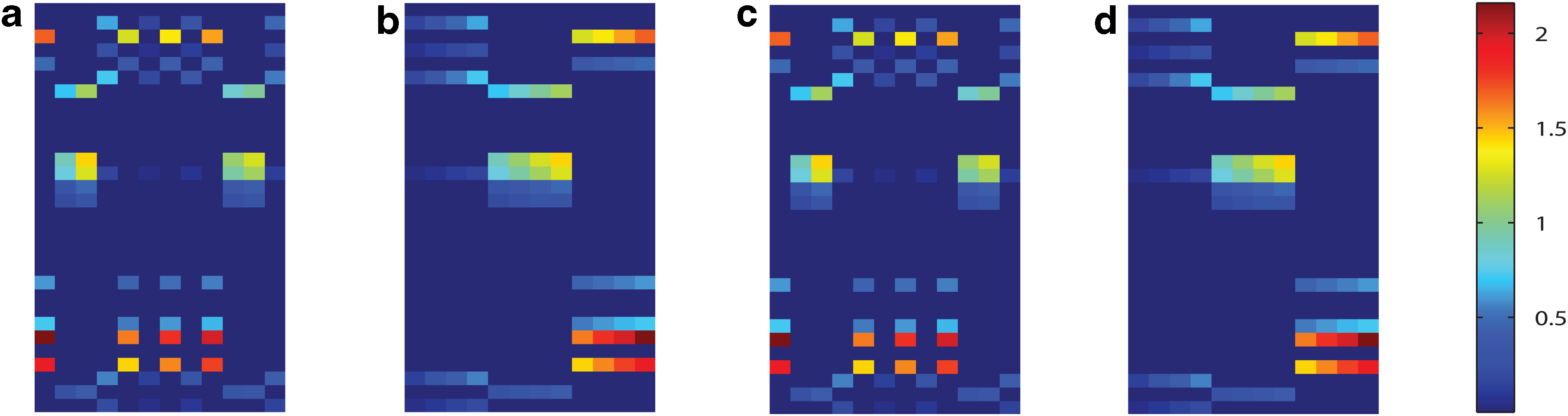
Figure 2a shows the original Wo matrix, where weight matrices in different time points are arranged in a column order. According to the construction process of Wo, tasks in Wo should form three low-rank subspaces. For easily visualizing this low-rank structure, we reshuffled tasks in Wo by putting tasks in the same group together and formed Figure 2b. Now the low-rank structure within the synthetic data can be easily detected, where every four columns in Figure 2b make a low-rank subspace. We applied our method to this synthetic data and plotted our learned W matrix in Figure 2c. To evaluate the structure of W, we did the rearrangement likewise. By comparing Figure 2b and d, we note that our method has successfully uncovered the group structure of the synthetic data and recovered the parameter matrix W in an accurate way.
Visualization of the synthetic parameter matrix W. Columns of W denote 12 prediction tasks from 4 different time points, whereas rows of W correspond to 30 features. These 12 tasks are equally divided into 3 groups, where tasks in the same group are identical to each other up to a scaling factor. (a) The original weight matrix Wo. (b) Rearrangement of columns in Wo by putting tasks in the same group together, such that the low-rank structure of Wo is more clear. (c) The learned W matrix by our model. (d) Rearrangement of W learned by our model.
5.2. Experimental settings on real benchmark data
In the following we evaluate our method on real benchmark datasets. We compare our method with all the counterparts discussed in the introduction section, which are: multivariate linear regression (LR), multivariate ridge regression (RR), multitask trace-norm regression (MTT) (Ji and Ye, 2009), Multitask \documentclass{aastex}\usepackage{amsbsy}\usepackage{amsfonts}\usepackage{amssymb}\usepackage{bm}\usepackage{mathrsfs}\usepackage{pifont}\usepackage{stmaryrd}\usepackage{textcomp}\usepackage{portland, xspace}\usepackage{amsmath, amsxtra}\usepackage{upgreek}\pagestyle{empty}\DeclareMathSizes{10}{9}{7}{6}\begin{document}
$${ \ell _{2 , 1}}$$
\end{document}-norm Regression (MTL21) (Evgeniou and Pontil, 2007), and their combination (MTT+L21) (Wang et al., 2012a,b).
In our preexperiments, we found the performance of our method to be relatively stable with parameters in the reasonable range (data not shown). For simplicity, we set \documentclass{aastex}\usepackage{amsbsy}\usepackage{amsfonts}\usepackage{amssymb}\usepackage{bm}\usepackage{mathrsfs}\usepackage{pifont}\usepackage{stmaryrd}\usepackage{textcomp}\usepackage{portland, xspace}\usepackage{amsmath, amsxtra}\usepackage{upgreek}\pagestyle{empty}\DeclareMathSizes{10}{9}{7}{6}\begin{document}
$${ \gamma _1} = 1$$
\end{document}, \documentclass{aastex}\usepackage{amsbsy}\usepackage{amsfonts}\usepackage{amssymb}\usepackage{bm}\usepackage{mathrsfs}\usepackage{pifont}\usepackage{stmaryrd}\usepackage{textcomp}\usepackage{portland, xspace}\usepackage{amsmath, amsxtra}\usepackage{upgreek}\pagestyle{empty}\DeclareMathSizes{10}{9}{7}{6}\begin{document}
$${ \gamma _2} = 1$$
\end{document}, \documentclass{aastex}\usepackage{amsbsy}\usepackage{amsfonts}\usepackage{amssymb}\usepackage{bm}\usepackage{mathrsfs}\usepackage{pifont}\usepackage{stmaryrd}\usepackage{textcomp}\usepackage{portland, xspace}\usepackage{amsmath, amsxtra}\usepackage{upgreek}\pagestyle{empty}\DeclareMathSizes{10}{9}{7}{6}\begin{document}
$$p = 0.8$$
\end{document}, \documentclass{aastex}\usepackage{amsbsy}\usepackage{amsfonts}\usepackage{amssymb}\usepackage{bm}\usepackage{mathrsfs}\usepackage{pifont}\usepackage{stmaryrd}\usepackage{textcomp}\usepackage{portland, xspace}\usepackage{amsmath, amsxtra}\usepackage{upgreek}\pagestyle{empty}\DeclareMathSizes{10}{9}{7}{6}\begin{document}
$$q = 0.1$$
\end{document}, and \documentclass{aastex}\usepackage{amsbsy}\usepackage{amsfonts}\usepackage{amssymb}\usepackage{bm}\usepackage{mathrsfs}\usepackage{pifont}\usepackage{stmaryrd}\usepackage{textcomp}\usepackage{portland, xspace}\usepackage{amsmath, amsxtra}\usepackage{upgreek}\pagestyle{empty}\DeclareMathSizes{10}{9}{7}{6}\begin{document}
$$k = 2.5$$
\end{document} without tuning. The definition and reasonable range of these parameters has been discussed in Section 4.
As the evaluation metric, we reported the root mean square error (RMSE) and correlation coefficient (CorCoe) between the predicted and actual scores in out-of-sample prediction. In our experiment, the RMSE was normalized by the Frobenius norm of the ground truth matrix. Better performance relates with lower RMSE or higher CorCoe value. We utilized the fivefold cross validation technique and reported the average RMSE and CorCoe on these five trials for each method.
5.3. Description of ADNI data
Data used in this work were obtained from the ADNI database (adni.loni.usc.edu). One goal of ADNI is to test whether serial magnetic resonance imaging (MRI), positron emission tomography (PET), other biological markers, and clinical and neuropsychological assessment can be combined to measure the progression of MCI and early AD. For up-to-date information, see www.adni-info.org.
The genotype data (Saykin et al., 2010) of all non-Hispanic Caucasian participants from the ADNI Phase 1 cohort were used in this study. They were genotyped using the Human 610-Quad BeadChip. Among all the SNPs, only SNPs, within the boundary of ±20 kbp base pairs of the 153 AD candidate genes listed on the AlzGene database (www.alzgene.org) as of April 18, 2011 (Bertram et al., 2007), were selected after the standard quality control (QC) and imputation steps. The QC criteria for the SNP data include (1) call rate check per subject and per SNP marker, (2) gender check, (3) sibling pair identification, (4) the Hardy–Weinberg equilibrium test, (5) marker removal by the minor allele frequency, and (6) population stratification. As the second preprocessing step, the QC'ed SNPs were imputed using the MaCH software (Li et al., 2010) to estimate the missing genotypes. As a result, our analyses included 3576 SNPs extracted from 153 genes (boundary: ±20 kbp) using the ANNOVAR annotation (www.openbioinformatics.org/annovar/).
Two widely employed automated MRI analysis techniques were used to process and extract imaging phenotypes from scans of ADNI participants as previously described (Shen et al., 2010). First, Voxel-Based Morphometry (VBM) (Ashburner and Friston, 2000) was performed to define global gray matter (GM) density maps and extract local GM density values for 90 target regions. Second, automated parcellation through FreeSurfer V4 (Fischl et al., 2002) was conducted to define volumetric and cortical thickness values for 90 regions of interest (ROIs) and to extract total intracranial volume (ICV). Further details are available in Shen et al. (2010). All these measures were adjusted for the baseline ICV using the regression weights derived from the healthy control (HC) participants. The time points examined in this study for imaging markers included baseline (BL), Month 6 (M6), Month 12 (M12), and Month 24 (M24). All the participants with no missing BL/M6/M12/M24 MRI measurements were included in this study, including 96 AD samples, and 219 MCI samples and 174 HC samples.
5.4. Performance comparison on ADNI cohort
In this study, we assessed the ability of our method to predict a set of imaging biomarkers through genetic variations. We tracked the process along the time axis and intended to uncover the latent subspace structure maintained by phenotypes and meanwhile capture a subset of SNPs influencing the phenotypes in a certain subspace.
We examined the cases where the number of selected SNPs were {30, 40, …, 80}. The experimental results are summarized in Tables 1 and 2. We observe that our method consistently outperforms other methods in most cases. The reasons go as follows: multivariate regression and ridge regression assumed the imaging features at different time points to be independent, thus did not consider the correlations within. Their neglects of the interrelations among the data were detrimental to their prediction performance.
Biomarker “VBM” and “FreeSurfer” (upper table for “VBM,” lower table for “FreeSurfer”) Prediction Comparison through Root Mean Square Error Measurement with Different Number of Selected SNPs
No. of SNPs
LR
RR
MTT
MTL21
MTT+L21
OURS
30
0.9277 ± 0.0122
0.9278 ± 0.0122
0.9270 ± 0.0135
0.9278 ± 0.0122
0.9276 ± 0.0126
0.9266 ± 0.0124
40
0.9106 ± 0.0147
0.9100 ± 0.0146
0.9099 ± 0.0141
0.9100 ± 0.0146
0.9099 ± 0.0141
0.9061 ± 0.0087
50
0.8914 ± 0.0177
0.8916 ± 0.0176
0.8934 ± 0.0159
0.8916 ± 0.0176
0.8919 ± 0.0176
0.8913 ± 0.0084
60
0.8843 ± 0.0216
0.8846 ± 0.0216
0.8831 ± 0.0192
0.8846 ± 0.0216
0.8848 ± 0.0215
0.8726 ± 0.0051
70
0.8661 ± 0.0204
0.8663 ± 0.0203
0.8675 ± 0.0211
0.8663 ± 0.0203
0.8666 ± 0.0202
0.8615 ± 0.0045
80
0.8509 ± 0.0250
0.8503 ± 0.0244
0.8500 ± 0.0242
0.8503 ± 0.0244
0.8500 ± 0.0242
0.8482 ± 0.0042
30
0.9667 ± 0.0145
0.9664 ± 0.0145
0.9667 ± 0.0145
0.9664 ± 0.0145
0.9664 ± 0.0146
0.9558 ± 0.0147
40
0.9569 ± 0.0113
0.9569 ± 0.0112
0.9569 ± 0.0113
0.9569 ± 0.0112
0.9569 ± 0.0114
0.9436 ± 0.0113
50
0.9502 ± 0.0141
0.9503 ± 0.0141
0.9502 ± 0.0141
0.9503 ± 0.0141
0.9503 ± 0.0142
0.9350 ± 0.0143
60
0.9416 ± 0.0106
0.9417 ± 0.0106
0.9416 ± 0.0106
0.9417 ± 0.0106
0.9415 ± 0.0107
0.9234 ± 0.0106
70
0.9319 ± 0.0105
0.9316 ± 0.0105
0.9319 ± 0.0105
0.9316 ± 0.0105
0.9321 ± 0.0106
0.9096 ± 0.0106
80
0.9246 ± 0.0093
0.9247 ± 0.0093
0.9246 ± 0.0093
0.9247 ± 0.0093
0.9247 ± 0.0094
0.9012 ± 0.0094
Better performance corresponds to lower root mean square error.
LR, linear regression; MTT, multitask trace-norm regression; RR, ridge regression; OURS, the proposed temporal structure auto-learning predictive model; SNPs, single nucleotide polymorphisms; VBM, Voxel-Based Morphometry.
Biomarker “VBM” and “FreeSurfer” (upper table for “VBM,” lower table for “FreeSurfer”) Prediction Comparison via Correlation Coefficient Measurement with Different Number of Selected SNPs
No. of SNPs
LR
RR
MTT
MTL21
MTT+L21
OURS
30
0.4186 ± 0.0092
0.4180 ± 0.0098
0.4232 ± 0.0088
0.4180 ± 0.0098
0.4216 ± 0.0077
0.6193 ± 0.0177
40
0.4284 ± 0.0163
0.4282 ± 0.0166
0.4333 ± 0.0181
0.4282 ± 0.0166
0.4312 ± 0.0157
0.6294 ± 0.0071
50
0.4476 ± 0.0395
0.4470 ± 0.0400
0.4526 ± 0.0384
0.4470 ± 0.0400
0.4508 ± 0.0385
0.6362 ± 0.0094
60
0.4477 ± 0.0391
0.4471 ± 0.0397
0.4513 ± 0.0388
0.4471 ± 0.0397
0.4510 ± 0.0380
0.6435 ± 0.0196
70
0.4502 ± 0.0345
0.4490 ± 0.0356
0.4547 ± 0.0335
0.4490 ± 0.0356
0.4529 ± 0.0339
0.6460 ± 0.0129
80
0.4467 ± 0.0287
0.4470 ± 0.0286
0.4514 ± 0.0271
0.4470 ± 0.0286
0.4508 ± 0.0268
0.6521 ± 0.0083
30
0.9007 ± 0.0145
0.9008 ± 0.0145
0.9007 ± 0.0145
0.9008 ± 0.0145
0.9010 ± 0.0146
0.9019 ± 0.0147
40
0.9049 ± 0.0113
0.9051 ± 0.0112
0.9049 ± 0.0113
0.9051 ± 0.0112
0.9052 ± 0.0114
0.9060 ± 0.0113
50
0.9045 ± 0.0141
0.9046 ± 0.0141
0.9045 ± 0.0141
0.9046 ± 0.0141
0.9048 ± 0.0142
0.9057 ± 0.0143
60
0.9079 ± 0.0106
0.9080 ± 0.0106
0.9079 ± 0.0106
0.9080 ± 0.0106
0.9081 ± 0.0107
0.9089 ± 0.0106
70
0.9094 ± 0.0105
0.9096 ± 0.0105
0.9094 ± 0.0105
0.9096 ± 0.0105
0.9097 ± 0.0106
0.9106 ± 0.0106
80
0.9114 ± 0.0093
0.9115 ± 0.0093
0.9114 ± 0.0093
0.9115 ± 0.0093
0.9117 ± 0.0094
0.9124 ± 0.0094
Better performance corresponds to higher correlation coefficient.
As for MTTrace, MTL21 and their combination MTTrace+MTL21, even though they take into account the inner connection information of imaging phenotypes, they simply constrain all phenotypes to a global space thus cannot handle the possible group structure therein. That is why they may overweigh the standard methods in some cases, but cannot outperform our proposed method. As for our proposed method, not only did we capture the latent structure among the longitudinal phenotypes, but we also selected a set of responsible SNPs at the same time. All in all, our model can capture SNPs responsible for some but not necessarily all imaging phenotypes along the time continuum, which save more effective information in the prediction.
5.5. Experiments on convergence analysis
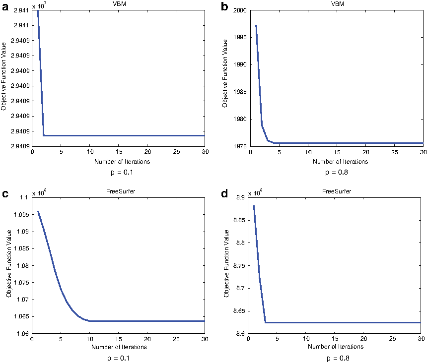
We applied our method to the ADNI cohort with two p-values (i.e., 0.1 and 0.8), and recorded the objective values of our proposed model in Equation (12) in each iteration. As shown in Figure 3, no matter what the p-value is, our model always converges within 10 iterations.
Objective function value of our proposed model in Equation (12) in each iteration with different p-values in the experiments on “VBM” biomarker (a, b) and “FreeSurfer” biomarker (c, d). VBM, Voxel-Based Morphometry.
5.6. Identification of top selected SNPs
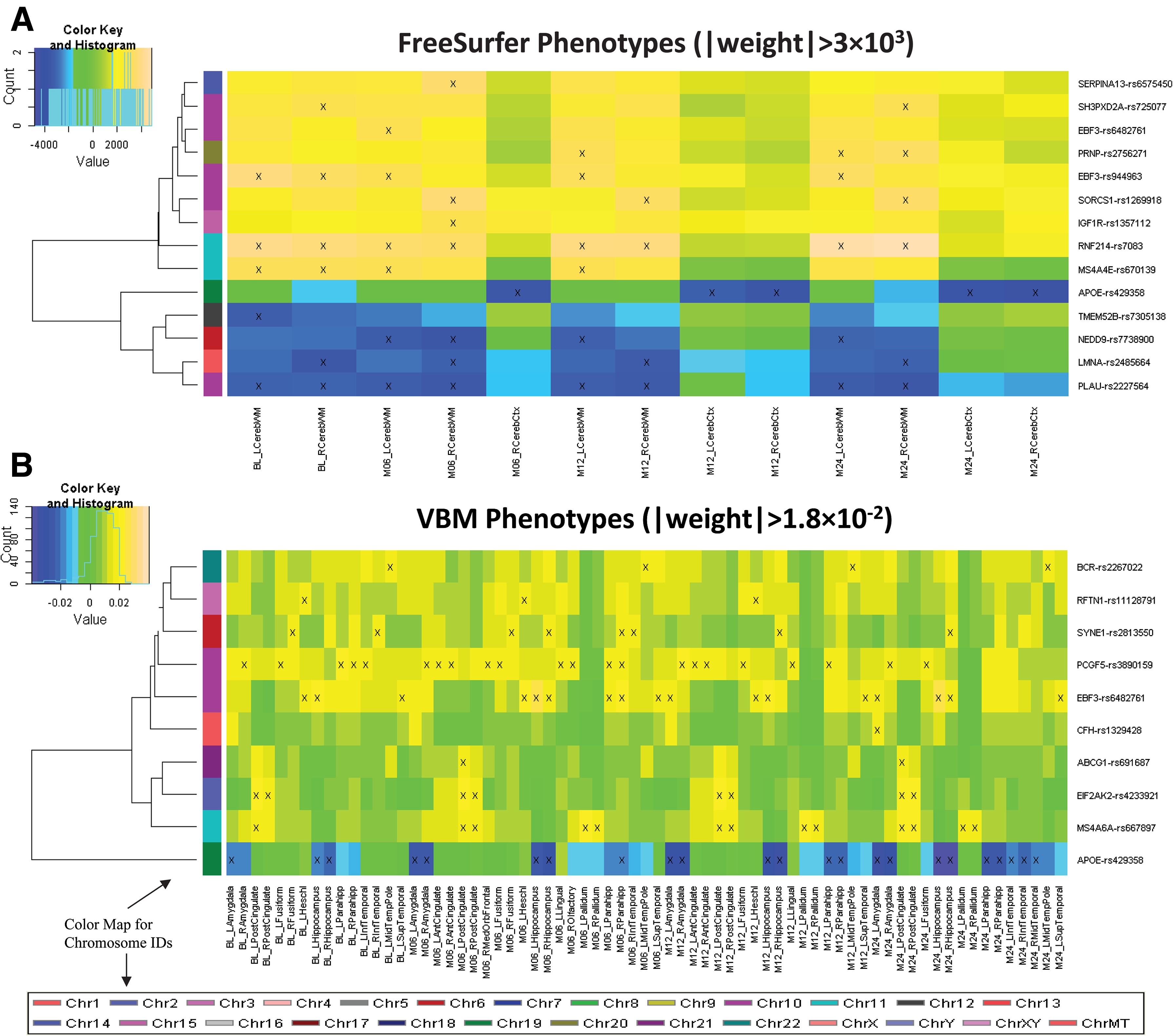
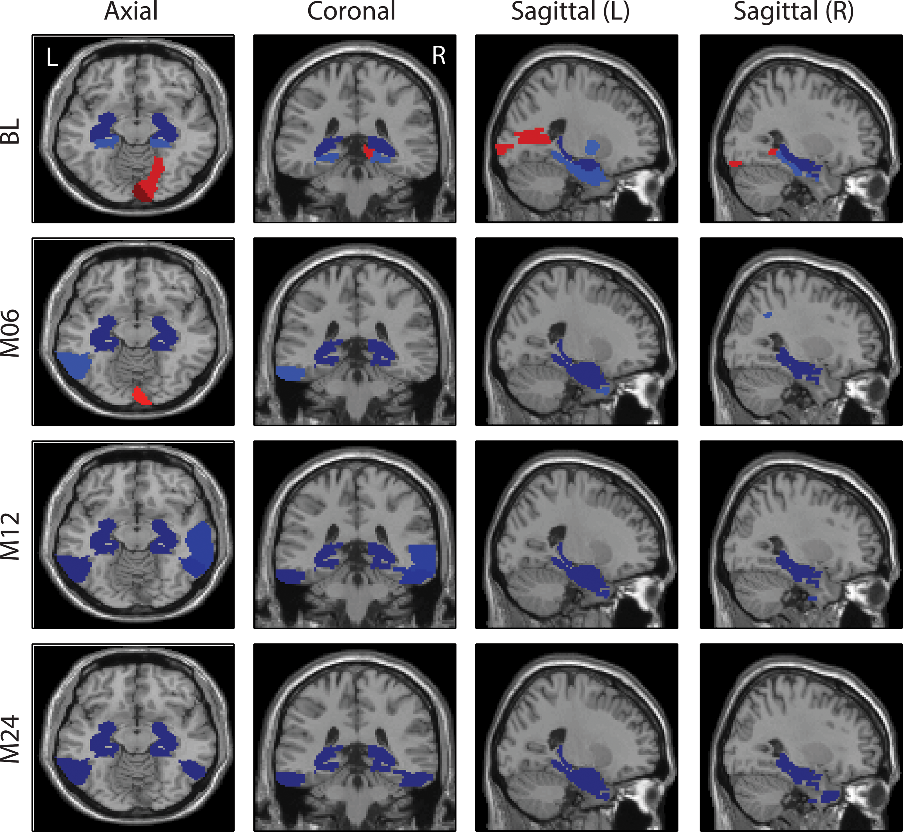
Shown in Figure 4 are the heat maps of top regression weights between imaging QTs and SNPs. APOE-rs429358, the well-known major AD risk factor, demonstrated relatively strong predictive power in both analyses: (1) In FreeSurfer analysis, it predicts mainly the cerebral cortex volume at M06, M12, and M24. (2) In VBM analysis, it predicts the GM densities of amygdala, hippocampus, and parahippocampal gyrus at multiple time points (Fig. 5). Both patterns are reassuring, since APOE-rs429358 and atrophy patterns of the entire cortex as well as medial temporal regions (including amygdala, hippocampus, and parahippocampal gyrus) are all highly associated with AD.
Heat maps of top regression weights between QTs and SNPs filtered by a user-specified weight threshold: (A) FreeSurfer QTs and (B) VBM QTs. Weights from each regression analysis are color mapped and displayed in the heat maps. Heat map blocks labeled with “x” reach the weight threshold. Only top SNPs and QTs are included in the heat maps, and so each row (SNP) and column (QT) have at least one “x” block. Dendrograms derived from hierarchical clustering are plotted for SNPs. The color bar on the left side of the heat map codes the chromosome IDs for the corresponding SNPs. QTs, quantitative traits.
Top 10 weights of APOE-rs429358 mapped on the brain for the VBM analysis.
In addition, APOE-rs429358 has been shown to be related to medial temporal lobe atrophy (Pereira et al., 2014), hippocampal atrophy (Andrawis et al., 2012), and cortical atrophy (Risacher et al., 2013). Variants within membrane-spanning 4-domains subfamily A (MS4A) gene cluster are some other recently discovered AD risk factors (Ma et al., 2014). Our analysis also demonstrated their associations with imaging QTs: (1) MS4A4E-rs670139 predicts cerebral white matter volume at BL, M06, and M12; and (2) MS4A6A-rs667897 predicts GM densities of posterior cingulate and pallidum at almost all time points. Another interesting finding is EBF3-rs482761, which is identified in both analyses: (1) In FreeSurfer analysis, it predicts left cerebral white matter volume at M06; and (2) in VBM analysis, it predicts GM densities of left Heschl's gyri, left superior temporal gyri, hippocampus, and left amygdala at multiple time points. EBF3 (early B-cell factor 3) is a protein-coding gene and has been associated with neurogenesis and glioblastoma. In general, both FreeSurfer and VBM analyses picked up similar regions across different time points. These identified imaging genomic associations warrant further investigation in independent cohorts. If replicated, these findings can potentially contribute to biomarker discovery for diagnosis and drug design.
6. Conclusions
In this article, we proposed a novel temporal structure auto-learning model to study the associations between genetic variations and longitudinal imaging phenotypes. Our model can simultaneously uncover the interrelation structures existing in different prediction tasks and utilize such learned interrelated structures to enhance the feature learning model. Moreover, we utilized the Schatten p-norm to extract the common subspace shared by the prediction tasks. Our new model is applied to ADNI cohort for neuroimaging phenotypes prediction through SNPs. We conducted experiments on both synthetic and real benchmark data. Empirical results validated the effectiveness of our model by demonstrating the improved prediction performance compared with related methods. In real data analysis, we also identified a set of interesting and biologically meaningful imaging genomic associations, showing the potential for biomarker discovery in disease diagnosis and drug design.
Footnotes
Acknowledgments
This work was partially supported by the National Science Foundation [IIS 1302675 to H.H., IIS 1344152 to H.H., DBI 1356628 to H.H., IIS 1619308 to H.H., and IIS 1633753 to H.H.] at PITT and [IIS 1622526 to L.S.] at IU; and by the National Institutes of Health [R01 LM011360 to L.S. and A.S., U01 AG024904 to Michael Weiner and A.S., RC2 AG036535 to Michael Weiner and A.S., R01 AG19771 to A.S., P30 AG10133 to A.S., and UL1 TR001108 to Anantha Shekhar], and [R01 AG049371 to H.H.] at PITT.
Author Disclosure Statement
The authors declare that no competing financial interests exist.
AndrawisJ.P., HwangK.S., GreenA.E., et al.2012. Effects of ApoE4 and maternal history of dementia on hippocampal atrophy. Neurobiol. Aging, 33, 856–866.
AshfordJ.W., and SchmittF.A.2001. Modeling the time-course of Alzheimer dementia. Curr. Psychiatry Rep. 3, 20–28.
5.
BentlerP.M., and LeeS.-Y.1978. Matrix derivatives with chain rule and rules for simple, Hadamard, and Kronecker products. J. Math. Psychol. 17, 255–262.
6.
BertramL., McQueenM.B., MullinK., et al.2007. Systematic meta-analyses of Alzheimer disease genetic association studies: The AlzGene database. Nat. Genet. 39, 17–23.
7.
BezdekJ.C., and HathawayR.J.2003. Convergence of alternating optimization. Neural Parallel Sci. Comput., 11, 351–368.
8.
BisJ.C., DeCarliC., SmithA.V., et al.2012. Common variants at 12q14 and 12q24 are associated with hippocampal volume. Nat. Genet. 44, 545–551.
9.
BurnsA., and IliffeS.2009. Alzheimer's disease. Br. Med. J. 338, b158.
10.
CaiT.T., and ZhangA.2013. Sharp RIP bound for sparse signal and low-rank matrix recovery. Appl. Comput. Harmon. Anal. 35, 74–93.
11.
CandèsE.J.2008. The restricted isometry property and its implications for compressed sensing. C. R. Math. 346, 589–592.
FischlB., SalatD.H., BusaE., et al.2002. Whole brain segmentation: Automated labeling of neuroanatomical structures in the human brain. Neuron, 33, 341–355.
14.
HaririA.R., DrabantE.M., and WeinbergerD.R.2006. Imaging genetics: Perspectives from studies of genetically driven variation in serotonin function and corticolimbic affective processing. Biol. Psychiatry, 59, 888–897.
15.
HaroldD., AbrahamR., HollingworthP., et al.2009. Genome-wide association study identifies variants at CLU and PICALM associated with Alzheimer's disease. Nat. Genet., 41, 1088–1093.
16.
JiS., and YeJ.2009. An accelerated gradient method for trace norm minimization, 457–464. In Proceedings of the 26th Annual International Conference on Machine Learning. ACM.
17.
KhachaturianZ.S.1985. Diagnosis of Alzheimer's disease. Arch. Neurol., 42, 1097–1105.
18.
KimS., SohnK.-A., and XingE.P.2009. A multivariate regression approach to association analysis of a quantitative trait network. Bioinformatics, 25, i204–i212.
19.
LiY., WillerC.J., DingJ., et al.2010. MaCH: Using sequence and genotype data to estimate haplotypes and unobserved genotypes. Genet. Epidemiol. 34, 816–834.
20.
MaJ., YuJ.T., and TanL.2014. MS4A cluster in Alzheimer's disease. Mol. Neurobiol., 51, 1240–1248.
21.
NieF., HuangH., and DingC.H.Q.2012. Low-rank matrix recovery via efficient schatten p-norm minimization. In AAAI Conference on Artificial Intelligence. AAAI Press.
PereiraJ.B., CavallinL., SpulberG., et al.2014. Influence of age, disease onset and ApoE4 on visual medial temporal lobe atrophy cut-offs. J. Intern. Med., 275, 317–330.
24.
PetrellaJ.R., ColemanR.E., and DoraiswamyP.M.2003. Neuroimaging and early diagnosis of Alzheimer disease: A look to the future 1. Radiology, 226, 315–336.
25.
PotkinS.G., GuffantiG., LakatosA., et al.2009a. Hippocampal atrophy as a quantitative trait in a genome-wide association study identifying novel susceptibility genes for Alzheimer's disease. PLoS One, 4, e6501.
26.
PotkinS.G., TurnerJ.A., GuffantiG., et al.2009b. Genome-wide strategies for discovering genetic influences on cognition and cognitive disorders: Methodological considerations. Cogn. Neuropsychiatry, 14, 391–418.
27.
RisacherS.L., KimS., ShenL., et al.2013. The role of apolipoprotein E (APOE) genotype in early mild cognitive impairment (E-MCI). Front. Aging Neurosci. 5, 11.
28.
RockafellarR.T.1970. Convex Analysis (Princeton Mathematical Series). Princeton University Press, 46:49.
29.
RuheA.1970. Perturbation bounds for means of eigenvalues and invariant subspaces. BIT Numer. Math., 10, 343–354.
30.
SabattiC., ServiceS.K., HartikainenA.L., et al.2008. Genome-wide association analysis of metabolic traits in a birth cohort from a founder population. Nat. Genet., 41, 35–46.
31.
SaykinA. J., ShenL., ForoudT.M., et al.2010. Alzheimer's Disease Neuroimaging Initiative biomarkers as quantitative phenotypes: Genetics core aims, progress, and plans. Alzheimer's Dement. 6, 265–273.
32.
ShenL., KimS., RisacherS.L., et al.2010. Whole genome association study of brain-wide imaging phenotypes for identifying quantitative trait loci in MCI and AD: A study of the ADNI cohort. Neuroimage, 53, 1051–1063.
WangH., NieF., HuangH., et al.2012a. From phenotype to genotype: An association study of longitudinal phenotypic markers to Alzheimer's disease relevant SNPs. Bioinformatics, 28, i619–i625.
35.
WangH., NieF., HuangH., et al.2012b. High-order multi-task feature learning to identify longitudinal phenotypic markers for Alzheimer's disease progression prediction, 1277–1285. In Advances in Neural Information Processing Systems. NIPS.
36.
WenkG.L.2003. Neuropathologic changes in Alzheimer's disease. J. Clin. Psychiatry. 64, 7–10.