Efficient Modeling and Simulation of Space-Dependent Biological Systems

Abstract

We recently demonstrated the possibility to model and to simulate biological functions using hardware description languages (HDLs) and associated simulators traditionally used for microelectronics. Nevertheless, those languages are not suitable to model and simulate space-dependent systems described by partial differential equations. However, in more and more applications space- and time-dependent models are unavoidable. For this purpose, we investigated a new modeling approach to simulate molecular diffusion on a mesoscopic scale still based on HDL. Our work relies on previous investigations on an electrothermal simulation tool for integrated circuits, and analogies that can be drawn between electronics, thermodynamics, and biology. The tool is composed of four main parts: a simple but efficient mesher that divides space into parallelepipeds (or rectangles in 2D) of adaptable size, a set of interconnected biological models, a SPICE simulator that handles the model and Python scripts that interface the different tools. Simulation results obtained with our tool have been validated on simple cases for which an analytical solution exists and compared with experimental data gathered from literature. Compared with existing approaches, our simulator has three main advantages: a very simple algorithm providing a direct interface between the diffusion model and biological model of each cell, the use of a powerful and widely proven simulation core (SPICE) and the ability to interface biological models with other domains of physics, enabling the study of transdisciplinary systems.

1. Introduction

Simulation of biological and biochemical systems aims at reproducing in silico various biological behaviors at different scales (molecules, cells, tissues, organs) to study them, better understand them, or predict the impact of external stimuli (environmental cues) or internal alterations (modification of mechanisms, addition/deletion of components, etc.). Up to now, hundreds of simulation tools dedicated to biology have been developed, mostly by academics. Some of them are dedicated to very specific needs, whereas others are generic and may be applied to a wider set of problems.

In this article, emphasis is put on the deterministic simulation of biological systems. In this case, a network of interactions between biochemical species needs to be simulated. This network is modeled by a set of ordinary differential equations (ODEs), that is, differential equations for which parameters, species concentration, and flux vary only with time. The ODE set is solved by a numerical method to obtain the temporal evolution of the system from a given initial state or under given stimuli. It may also provide the steady states of the system as a function of its biochemical parameters or even identify mathematical properties of the studied network. Such models can be handled either by generic calculation tools such as MATLAB (Schmidt and Jirstrand, 2006) or specific packages of Python (Lopez et al., 2013), by dedicated tools such as COPASI (Hoops et al., 2006), BioCham (Calzone et al., 2006), or JSim (Butterworth et al., 2013) or by tools derived from other domains of engineering sciences such as SPICE, a language dedicated to the simulation of electronic circuits (Madec et al., 2017).

Aforementioned tools solve ODE, which implies that the system can be modeled with lumped quantities and parameters. However, it is not uncommon to encounter biochemical systems for which the spatial distribution of chemical species and/or local variations of biochemical properties play a significant role. This is the case in applications such as the diffusion of drugs in tissues (Arifin et al., 2006), the study of intercellular communication (Tamsir et al., 2011; Xie et al., 2011), or intracellular signaling (Goldbeter et al., 1990; Somogyi and Stucki, 1991). To tackle these questions, several approaches exist. Most of them have been summarized by Takahashi in a review article in 2005 (Takahashi et al., 2005).

Basically, two main approaches can be distinguished. On the one hand, each molecule is modeled individually. The position of each molecule as well as their interactions are computed. This approach is called entity-centered (or particle-centered). Various implementations of this approach exist, depending on the way the space and the position of entities are represented. In entity-centered simulator, such as HSIM (Amar et al., 2004), the coordinate of each molecule is updated according to a random walk at each time step and if the trajectories of two molecules involved in a reaction cross each other, the reaction has a probability to occur. Alternative implementations of this approach use cellular automata (Ermentrout and Edelstein-Keshet, 1993; Madec et al., 2012). In this case, space is divided into cubes. At each time step, transfers of molecules from one cube to another one and/or reactions between two molecules inside a cube are computed according to probabilistic laws.

On the other hand, geometry can be taken into account in models by considering the concentration of each species as a function of both time and space. In this case, the biological system is described as a set of partial differential equations (PDEs) composed of diffusion terms and reaction terms, which also may depend on the position in space. PDEs can be solved numerically by different methods such as finite differences, finite elements, finite volumes, etc. (Evans et al., 2000). These methods are the same as the ones encountered in other domains of physics, such as thermodynamics, flow mechanics, electromagnetism, or physics of semiconductor.

They can be handled by commercial software, such as COMSOL, which is a reference PDE solver in physics. Moreover, last distribution COMSOL include a module dedicated to the simulation of chemical reactions. They can also be solved using open-source C++ libraries, such FreeFEM (Hecht, 2012), or simulated with dedicated freeware such as Virtual Cell, a standard tool in system biology (Moraru and Schaff, 2008). Whatever the resolution method, space is discretized into meshes and nodes, and PDEs are converted in a set of ODEs, one per species and per nodes. Consequently, PDE solvers are composed of two parts: a mesher that converts PDEs into ODEs and an ODE solver. The performance of a given method is always a tradeoff between accuracy and computation time. High accuracy can be reached with very tight meshes and/or sophisticated discretization schemes and ODE-solving method (e.g., finite elements), but the price to pay is an increase in the number of equations to solve, the size of the data to store, and the complexity of the equations.

From a mathematical point of view, PDE-based biological models are close to those met in electrothermal simulations of integrated circuits. In this domain, efficient methods have already been proven for years to handle these models (Vogelsong and Brzezinski, 1989; Digele et al., 1997; Wunsche et al., 1997; Krencker et al., 2010, 2014; Garci et al., 2014). The tool described in this article is an adaptation of the tool developed by Krencker and Garci to the biological domain. This adaptation is made possible, thanks to analogies that exist among biology, electronics, and thermodynamics. The first section of the article introduces the background of the article, that is, the modeling of diffusion in biology and the aforementioned analogies. The tool is described in detail in Section 3. Then, simulation results, validations, and comparisons with experimental data extracted from the literature are given in Section 4. Finally, the performances obtained with our approach are discussed and compared with alternative solutions (namely COMSOL and Virtual Cell) in Section 5.

2. Theoretical Background

2.1. Space- and time-dependent models in biology

The generic model for a biological system that depends both on time and space is a set of PDEs (one per species), which can be written as following: \documentclass{aastex}\usepackage{amsbsy}\usepackage{amsfonts}\usepackage{amssymb}\usepackage{bm}\usepackage{mathrsfs}\usepackage{pifont}\usepackage{stmaryrd}\usepackage{textcomp}\usepackage{portland, xspace}\usepackage{amsmath, amsxtra}\usepackage{upgreek}\pagestyle{empty}\DeclareMathSizes{10}{9}{7}{6}\begin{document} \begin{align*} { \frac { \partial { X_k } } { \partial t } } = { f_k } \left( { { X_k } , t , x , y , z } \right) + \mathop \sum \limits_ { j = 1 } ^R { v_ { j , k } } \left( { { \bf { X } } , t , x , y , z } \right) - { d_k } \cdot { X_k } \left( { t , x , y , z } \right) \quad k = \left\{ { 1 \ldots N } \right\} \tag { 1 } \end{align*} \end{document}

where N is the number of involved species, \documentclass{aastex}\usepackage{amsbsy}\usepackage{amsfonts}\usepackage{amssymb}\usepackage{bm}\usepackage{mathrsfs}\usepackage{pifont}\usepackage{stmaryrd}\usepackage{textcomp}\usepackage{portland, xspace}\usepackage{amsmath, amsxtra}\usepackage{upgreek}\pagestyle{empty}\DeclareMathSizes{10}{9}{7}{6}\begin{document} $${ \bf{X}} \left( {t , x , y , z} \right)$$ \end{document} is a vector with N elements \documentclass{aastex}\usepackage{amsbsy}\usepackage{amsfonts}\usepackage{amssymb}\usepackage{bm}\usepackage{mathrsfs}\usepackage{pifont}\usepackage{stmaryrd}\usepackage{textcomp}\usepackage{portland, xspace}\usepackage{amsmath, amsxtra}\usepackage{upgreek}\pagestyle{empty}\DeclareMathSizes{10}{9}{7}{6}\begin{document} $${X_k} \left( {t , x , y , z} \right)$$ \end{document} , each being the concentration of the k-th species at time t and position \documentclass{aastex}\usepackage{amsbsy}\usepackage{amsfonts}\usepackage{amssymb}\usepackage{bm}\usepackage{mathrsfs}\usepackage{pifont}\usepackage{stmaryrd}\usepackage{textcomp}\usepackage{portland, xspace}\usepackage{amsmath, amsxtra}\usepackage{upgreek}\pagestyle{empty}\DeclareMathSizes{10}{9}{7}{6}\begin{document} $$\left( {x , y , z} \right)$$ \end{document} , R the number of biochemical reactions which influences the local concentrations, \documentclass{aastex}\usepackage{amsbsy}\usepackage{amsfonts}\usepackage{amssymb}\usepackage{bm}\usepackage{mathrsfs}\usepackage{pifont}\usepackage{stmaryrd}\usepackage{textcomp}\usepackage{portland, xspace}\usepackage{amsmath, amsxtra}\usepackage{upgreek}\pagestyle{empty}\DeclareMathSizes{10}{9}{7}{6}\begin{document} $${v_{j , k}} \left( {{ \bf{X}} , t , x , y , z} \right)$$ \end{document} is the rate at which the j-th reaction produces or consumes the k-th species, d_k is the degradation constant associated with the k-th species, and \documentclass{aastex}\usepackage{amsbsy}\usepackage{amsfonts}\usepackage{amssymb}\usepackage{bm}\usepackage{mathrsfs}\usepackage{pifont}\usepackage{stmaryrd}\usepackage{textcomp}\usepackage{portland, xspace}\usepackage{amsmath, amsxtra}\usepackage{upgreek}\pagestyle{empty}\DeclareMathSizes{10}{9}{7}{6}\begin{document} $${f_k} \left( {{X_k} , t , x , y , z} \right)$$ \end{document} is a term that models the diffusion of the k-th species into space. Generally, \documentclass{aastex}\usepackage{amsbsy}\usepackage{amsfonts}\usepackage{amssymb}\usepackage{bm}\usepackage{mathrsfs}\usepackage{pifont}\usepackage{stmaryrd}\usepackage{textcomp}\usepackage{portland, xspace}\usepackage{amsmath, amsxtra}\usepackage{upgreek}\pagestyle{empty}\DeclareMathSizes{10}{9}{7}{6}\begin{document} $${f_k} \left( {{X_k} , t , x , y , z} \right)$$ \end{document} corresponds to the Fick law (Fick, 1855): \documentclass{aastex}\usepackage{amsbsy}\usepackage{amsfonts}\usepackage{amssymb}\usepackage{bm}\usepackage{mathrsfs}\usepackage{pifont}\usepackage{stmaryrd}\usepackage{textcomp}\usepackage{portland, xspace}\usepackage{amsmath, amsxtra}\usepackage{upgreek}\pagestyle{empty}\DeclareMathSizes{10}{9}{7}{6}\begin{document} \begin{align*} { f_k } \left( { { X_k } , t , x , y , z } \right) = { D_k } \left( { t , x , y , z } \right) \cdot { \nabla ^2 } { X_k } = { D_k } \left( { t , x , y , z } \right) \cdot \left( { { \frac { { \partial ^2 } { X_k } } { \partial { x^2 } } } + { \frac { { \partial ^2 } { X_k } } { \partial { y^2 } } } + { \frac { { \partial ^2 } { X_k } } { \partial { z^2 } } } } \right) \tag { 2 } \end{align*} \end{document}

For the \documentclass{aastex}\usepackage{amsbsy}\usepackage{amsfonts}\usepackage{amssymb}\usepackage{bm}\usepackage{mathrsfs}\usepackage{pifont}\usepackage{stmaryrd}\usepackage{textcomp}\usepackage{portland, xspace}\usepackage{amsmath, amsxtra}\usepackage{upgreek}\pagestyle{empty}\DeclareMathSizes{10}{9}{7}{6}\begin{document} $${v_{j , k}}$$ \end{document} functions, standard models of biochemistry, such as Hill's equations (Konkoli, 2011), Michaelis–Menten's models (Michaelis and Maud Menten, 1913) or protein-binding polynomial (Haiech et al., 2014), are implemented. Such models may depend on the concentration of all other involved species, the time, and the position.

2.2. Analogy between electronic, thermic, and biology

On the one hand, the analogy between electronics and biology has been demonstrated in Gendrault et al. (2014). Basically, it consists in considering the concentration as an electrical voltage, the production/consumption of a species as a current source, the degradation term as a resistor, and the local storage of molecules as a capacitor. The current sources associated with species production/consumption may be controlled by other voltages, leading to the instantiation of voltage-controlled current sources (VCCS), just as in models of transistors in electronics. Based on this analogy, every biological system that does not depend on space can be modeled as equivalent electronic circuits. The mathematical equations that model the system in standard approach can be retrieved by applying Kirchhoff's laws to this circuit.

On the other hand, an analogy can be drawn between biology and thermal physics considering diffusion phenomena. The model of the thermal diffusion of heat in a material is given by heat equation, derived from Fourier's law (Blundell and Blundell, 2010): \documentclass{aastex}\usepackage{amsbsy}\usepackage{amsfonts}\usepackage{amssymb}\usepackage{bm}\usepackage{mathrsfs}\usepackage{pifont}\usepackage{stmaryrd}\usepackage{textcomp}\usepackage{portland, xspace}\usepackage{amsmath, amsxtra}\usepackage{upgreek}\pagestyle{empty}\DeclareMathSizes{10}{9}{7}{6}\begin{document} \begin{align*} C \left( { t , x , y , z } \right) \cdot { \frac { \partial T } { \partial t } } = { K_0 } \left( { t , x , y , z } \right) \cdot { \nabla ^2 } T + Q \left( { t , x , y , z } \right) - h \left( { t , x , y , z } \right) \cdot T \left( { t , x , y , z } \right) \tag { 3 } \end{align*} \end{document}

where \documentclass{aastex}\usepackage{amsbsy}\usepackage{amsfonts}\usepackage{amssymb}\usepackage{bm}\usepackage{mathrsfs}\usepackage{pifont}\usepackage{stmaryrd}\usepackage{textcomp}\usepackage{portland, xspace}\usepackage{amsmath, amsxtra}\usepackage{upgreek}\pagestyle{empty}\DeclareMathSizes{10}{9}{7}{6}\begin{document} $$T \left( {t , x , y , z} \right)$$ \end{document} is the temperature, \documentclass{aastex}\usepackage{amsbsy}\usepackage{amsfonts}\usepackage{amssymb}\usepackage{bm}\usepackage{mathrsfs}\usepackage{pifont}\usepackage{stmaryrd}\usepackage{textcomp}\usepackage{portland, xspace}\usepackage{amsmath, amsxtra}\usepackage{upgreek}\pagestyle{empty}\DeclareMathSizes{10}{9}{7}{6}\begin{document} $$C \left( {t , x , y , z} \right)$$ \end{document} is the local heat capacity, \documentclass{aastex}\usepackage{amsbsy}\usepackage{amsfonts}\usepackage{amssymb}\usepackage{bm}\usepackage{mathrsfs}\usepackage{pifont}\usepackage{stmaryrd}\usepackage{textcomp}\usepackage{portland, xspace}\usepackage{amsmath, amsxtra}\usepackage{upgreek}\pagestyle{empty}\DeclareMathSizes{10}{9}{7}{6}\begin{document} $${K_0} \left( {t , x , y , z} \right)$$ \end{document} is the thermal conductivity, \documentclass{aastex}\usepackage{amsbsy}\usepackage{amsfonts}\usepackage{amssymb}\usepackage{bm}\usepackage{mathrsfs}\usepackage{pifont}\usepackage{stmaryrd}\usepackage{textcomp}\usepackage{portland, xspace}\usepackage{amsmath, amsxtra}\usepackage{upgreek}\pagestyle{empty}\DeclareMathSizes{10}{9}{7}{6}\begin{document} $$Q \left( {t , x , y , z} \right)$$ \end{document} is the distribution of heat sources in space and time, and \documentclass{aastex}\usepackage{amsbsy}\usepackage{amsfonts}\usepackage{amssymb}\usepackage{bm}\usepackage{mathrsfs}\usepackage{pifont}\usepackage{stmaryrd}\usepackage{textcomp}\usepackage{portland, xspace}\usepackage{amsmath, amsxtra}\usepackage{upgreek}\pagestyle{empty}\DeclareMathSizes{10}{9}{7}{6}\begin{document} $$h \left( {t , x , y , z} \right)$$ \end{document} is the convection constant. Similarities between heat equation [Eq. (3)] and [Eq. (1)] with f corresponding to Fick's law [Eq. (2)] are obvious.

Finally, the analogy between electronics and thermal physics is also well known (Blundell and Blundell, 2010). Electrothermal simulations of integrated circuits are mostly based on this analogy.

2.3. Electrothermal simulation of integrated circuits

The electrothermal simulation of an integrated circuit is needed especially for high-density integrated circuits, for mixed circuits with integrated power devices, or for the next generation of 3D-integrated circuits. Such a simulation requires two modeling layers, one dedicated to the computation of the thermal map and one dedicated to the computation of the voltages and currents in the electronic circuit. The last generation of electrothermal simulator uses a direct coupling, that is, both layers are computed together with the same solver. The principle is described in Krencker et al. (2010). On the thermal layer, heat equation is discretized and modeled with electronic equivalent circuits. Such circuits are composed of thermal capacitor on each node of the lattice to model heat accumulation by the chip, thermal resistor between nodes to model the heat transfer, thermal resistor between nodes and the thermal ground (ambient temperature) to model heat convection, and localized heat sources. The electronic layer is composed of temperature-dependent models of devices instantiated in the circuit. Each model is connected to the closest thermal node, uses the node temperature inside models to set temperature-dependent parameters, and computes the localized heat source associated to the device.

3. Description of the Tool

The biological simulator described in this article is based on the same principle and relies on the aforementioned analogies. Since heat diffusion and molecule diffusion are modeled by similar laws on the one hand, and biological systems can be described as electronic circuits on the other hand, it is possible to describe a space- and time-dependent biological system as an equivalent electronic circuit composed of several layers of components. As for electrothermal simulator, the first layer is composed of local models of chemical reaction, which are modeled by electronic equivalent devices. However, unlike the electrothermal simulator, where only heat diffusion has to be modeled, molecular diffusion requires one layer per diffusing species. Those layers are mostly composed of resistors, capacitors, and VCCS to model fluxes between nodes. The model is written in SPICE. The complete tool is composed of four main modules: the mesher, the SPICE netlist generator, the models for the elementary mesh and biochemical reactions, and the SPICE simulator. In the following, for simplicity sake, only the case of 2D problems is addressed. Nevertheless, the mesher, the circuit model file generator, and the SPICE model for the elemental mesh have been developed to be compatible with 3D studies.

3.1. Mesher

The mesher is implemented in C++. It is a direct reuse of the mesher used for the electrothermal simulator (Krencker et al., 2010). To reduce the computation time and the complexity of the model, we opted for a lattice composed of square meshes with variable degrees of refinement. To generate the lattice, users have to provide in a text file the geometry, the maximal size of an element, and a list of critical zones in which mesh refinement is required for each species. It is obviously advisable to use influence zones close to the region where the variation of species concentration is significant (for instance in regions where the species are produced).

The mesher reads the input files and creates a list of mesh elements and their associated nodes, as well as a list of all node coordinates. The algorithm performs as following. First, a lattice made of squares of the maximal size defined by the user is generated. Then each square overlapping an influence zone is cut into four identical squares if its size is larger than the maximal size allowed inside this zone. This operation is repeated until all the squares overlapping an influence zone are smaller than the maximal size. Finally, the transitions between adjacent squares with different degrees of refinement are smoothed. If the difference of degrees of refinement of two adjacent squares is larger than 1, that is, when the ratio of their sides' sizes is larger than 2, the largest square is cut in four, and this last operation is also repeated until each couple of adjacent squares exhibit a difference of degrees of refinement of 1 or less (Fig. 1).

FIG. 1.

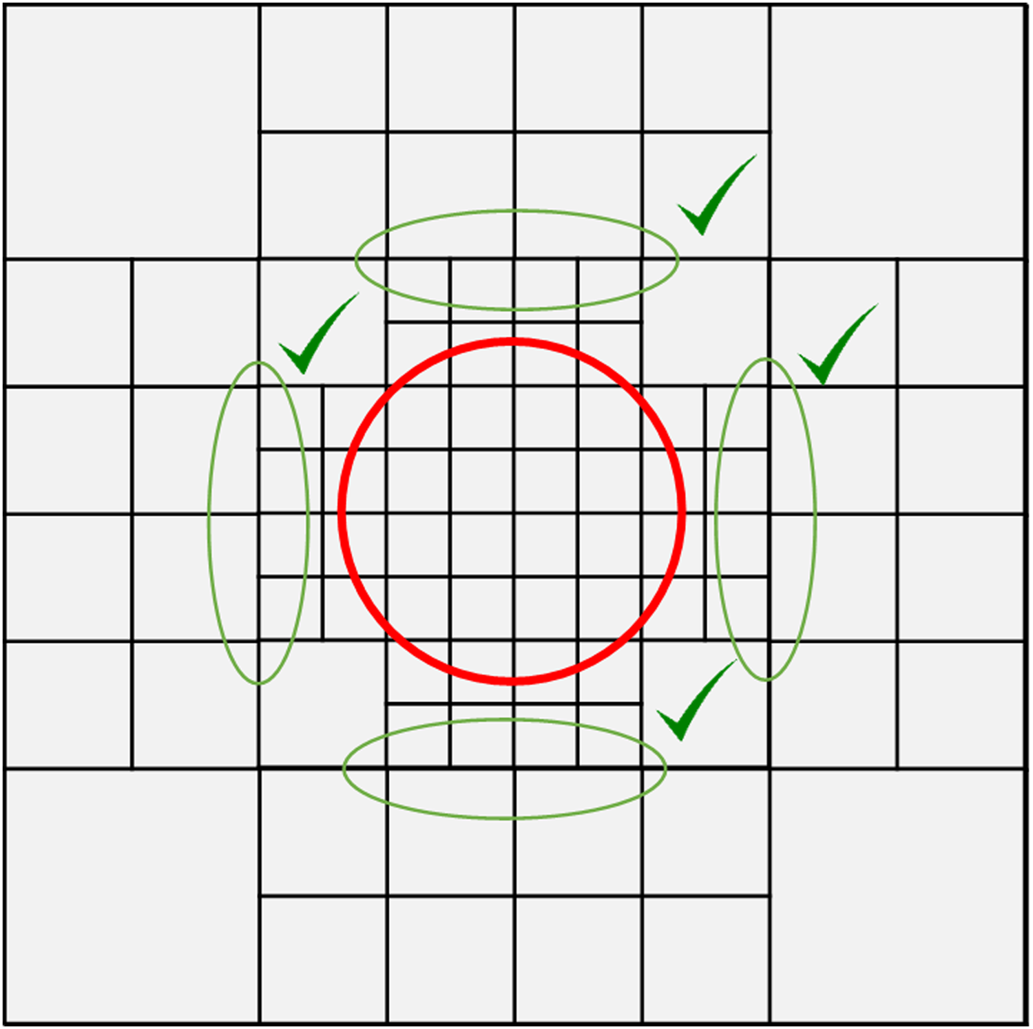
Example of a lattice with four initial divisions and with a central refinement zone of n = 2 (red circle). The algorithm checks whether the degree of refinement (n value) of each mesh in contact with the zone is greater or equal to the expected value (here 2). If not, the relevant meshes are subdivided. To keep a progressive refinement, some meshes have to be divided even if not in contact with the refining zone: green shapes illustrate this case.

3.2. SPICE netlist generator

The SPICE netlist generator is a Python script that generates a SPICE file describing the electronic equivalent model of the complete system. This file is composed of the following elements: (1) the definition of the global parameters of the model; (2) the instantiations of the elementary mesh models (described in more details in subsection 3.3); (3) the map of initial concentrations; (4) the boundary conditions; (5) the instantiations of SPICE models of local biological mechanisms; and (6) simulation directives. In the current version of the tool, models' parameters, the initial concentration map, boundary conditions, simulation directives, and the position of biological mechanisms have to be set using Python scripts given in Supplementary Material. The formalization of a metalanguage used to describe the system and that can be interpreted to generate the SPICE model is still under consideration.

For boundary conditions, several options are available. By default, the space represented by the lattice is considered as closed. From a modeling point of view, each boundary node is open. Constant concentration can also be applied on boundaries. In this case, boundary nodes are connected to constant voltage sources (or grounded if concentration is 0). Finally, it is also possible to model further diffusion outside the lattice borders by adding a grounded resistor to the concerned border nodes.

SPICE models of local biological mechanism can either be handwritten directly in SPICE or be exported from SBML (System Biology Markup Language, an XML-based standard description language used in biology) (Hucka, 2003) or from a textual description by using BB-SPICE (Madec et al., 2017).

3.3. Model of the elementary mesh

3.3.1. Model core

In 2D, the elementary mesh is a square with up to eight connections. Corners (C1, C2, C3, and C4) are defined in every mesh, whereas middles of edges (C12, C23, C34, C41) exist only if adjacent meshes are refined. The core of the model maps the discretization of Fick's law according to the finite differences scheme. It means that the application of Kirchhoff's law on each node of the mesh leads to a set of ODEs, which corresponds to the one obtained with the set of equations coming from discretizing [Eq. (1)] with Fick's law with the finite difference method. In the following, for simplicity's sake, the name of a node (e.g., C1) will implicitly correspond to the concentration of molecule on that node.

3.3.1.1. Discretization of diffusion term

When discretized, Fick's law leads to flow terms that depend on the concentrations at the corners of the mesh element. In 2D, we define four fluxes per mesh, two along the X-axis ( \documentclass{aastex}\usepackage{amsbsy}\usepackage{amsfonts}\usepackage{amssymb}\usepackage{bm}\usepackage{mathrsfs}\usepackage{pifont}\usepackage{stmaryrd}\usepackage{textcomp}\usepackage{portland, xspace}\usepackage{amsmath, amsxtra}\usepackage{upgreek}\pagestyle{empty}\DeclareMathSizes{10}{9}{7}{6}\begin{document} $${F_{12}}$$ \end{document} and \documentclass{aastex}\usepackage{amsbsy}\usepackage{amsfonts}\usepackage{amssymb}\usepackage{bm}\usepackage{mathrsfs}\usepackage{pifont}\usepackage{stmaryrd}\usepackage{textcomp}\usepackage{portland, xspace}\usepackage{amsmath, amsxtra}\usepackage{upgreek}\pagestyle{empty}\DeclareMathSizes{10}{9}{7}{6}\begin{document} $${F_{43}}$$ \end{document} ) and two along the Y-axis ( \documentclass{aastex}\usepackage{amsbsy}\usepackage{amsfonts}\usepackage{amssymb}\usepackage{bm}\usepackage{mathrsfs}\usepackage{pifont}\usepackage{stmaryrd}\usepackage{textcomp}\usepackage{portland, xspace}\usepackage{amsmath, amsxtra}\usepackage{upgreek}\pagestyle{empty}\DeclareMathSizes{10}{9}{7}{6}\begin{document} $${F_{14}}$$ \end{document} and \documentclass{aastex}\usepackage{amsbsy}\usepackage{amsfonts}\usepackage{amssymb}\usepackage{bm}\usepackage{mathrsfs}\usepackage{pifont}\usepackage{stmaryrd}\usepackage{textcomp}\usepackage{portland, xspace}\usepackage{amsmath, amsxtra}\usepackage{upgreek}\pagestyle{empty}\DeclareMathSizes{10}{9}{7}{6}\begin{document} $${F_{23}}$$ \end{document} ). Each flux is proportional to half of the gradient between both nodes (Fig. 2): \documentclass{aastex}\usepackage{amsbsy}\usepackage{amsfonts}\usepackage{amssymb}\usepackage{bm}\usepackage{mathrsfs}\usepackage{pifont}\usepackage{stmaryrd}\usepackage{textcomp}\usepackage{portland, xspace}\usepackage{amsmath, amsxtra}\usepackage{upgreek}\pagestyle{empty}\DeclareMathSizes{10}{9}{7}{6}\begin{document} \begin{align*} { F_ { ij } } = \frac { { { D_n } \cdot \left( { { C_i } - { C_j } } \right) } } { 2 } \tag { 4 } \end{align*} \end{document}

where D_n is the diffusion constant inside the mesh that depends on diffusion constant D₀, the size of the unrefined mesh \documentclass{aastex}\usepackage{amsbsy}\usepackage{amsfonts}\usepackage{amssymb}\usepackage{bm}\usepackage{mathrsfs}\usepackage{pifont}\usepackage{stmaryrd}\usepackage{textcomp}\usepackage{portland, xspace}\usepackage{amsmath, amsxtra}\usepackage{upgreek}\pagestyle{empty}\DeclareMathSizes{10}{9}{7}{6}\begin{document} $$M{S_0}$$ \end{document} , and the degree of refinement n of the mesh according to the following equation: \documentclass{aastex}\usepackage{amsbsy}\usepackage{amsfonts}\usepackage{amssymb}\usepackage{bm}\usepackage{mathrsfs}\usepackage{pifont}\usepackage{stmaryrd}\usepackage{textcomp}\usepackage{portland, xspace}\usepackage{amsmath, amsxtra}\usepackage{upgreek}\pagestyle{empty}\DeclareMathSizes{10}{9}{7}{6}\begin{document} \begin{align*} { D_n } = { D_0 } { \frac { { 2^ { n - 1 } } } { MS_0^2 } } \tag { 5 } \end{align*} \end{document}

FIG. 2.

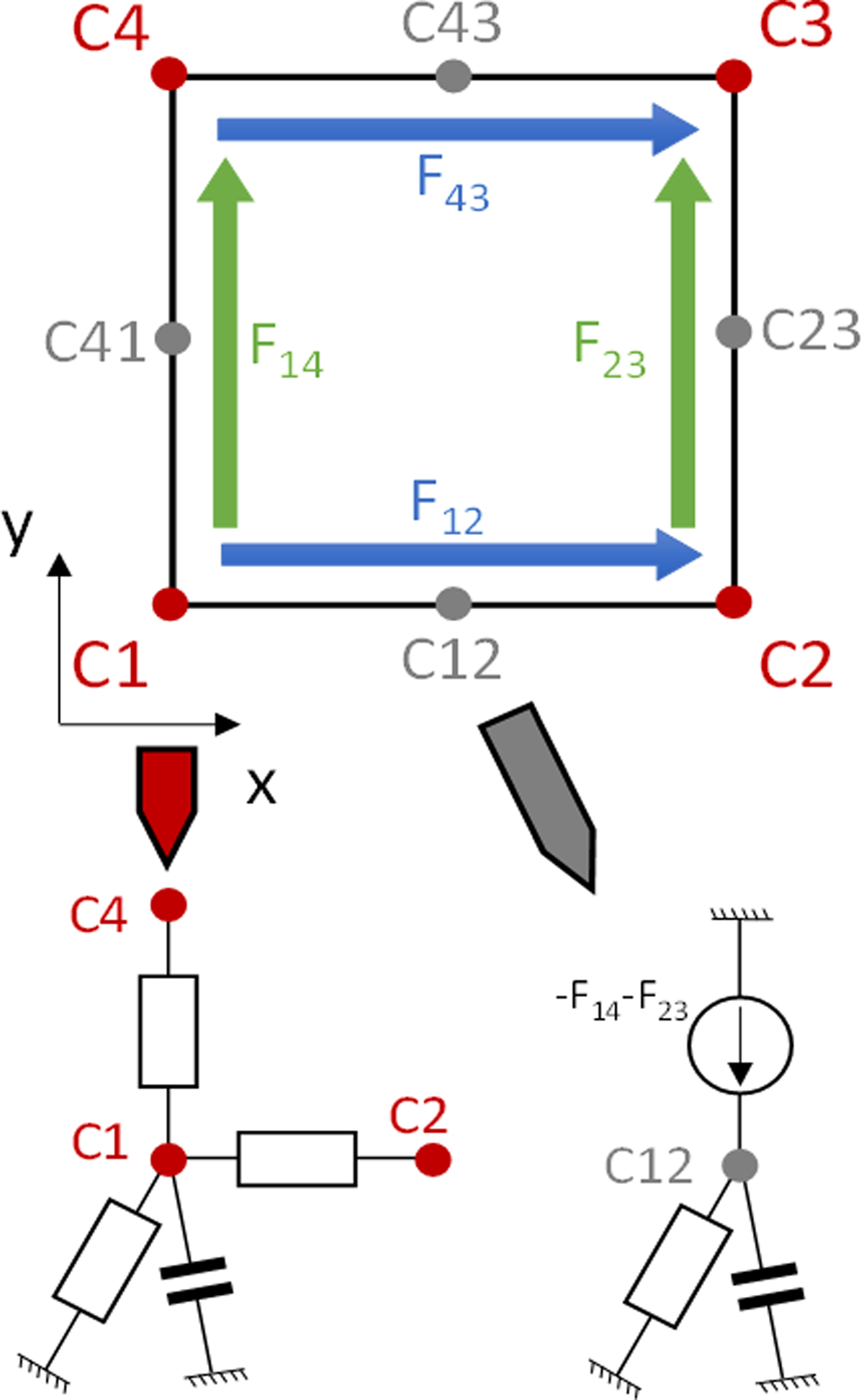
Upper part: 2D elementary mesh with eight potential connections: four corners (always connected, red dots) and four edges (not connected if the degree of refinement of the neighbor mesh is the same, gray dots). Plain arrows (blue and green) show the fluxes. Lower part: representation of the electronic devices connected to a corner node (left) or an edge node (right).

Each corner node receives two fluxes, one along each axis. Once the lattice is assembled, it should be noticed that each corner receives each flux twice, which explains why the flux is divided by 2 in [Eq. (4)]. For instance, C2 receives \documentclass{aastex}\usepackage{amsbsy}\usepackage{amsfonts}\usepackage{amssymb}\usepackage{bm}\usepackage{mathrsfs}\usepackage{pifont}\usepackage{stmaryrd}\usepackage{textcomp}\usepackage{portland, xspace}\usepackage{amsmath, amsxtra}\usepackage{upgreek}\pagestyle{empty}\DeclareMathSizes{10}{9}{7}{6}\begin{document} $${F_{12}}$$ \end{document} and \documentclass{aastex}\usepackage{amsbsy}\usepackage{amsfonts}\usepackage{amssymb}\usepackage{bm}\usepackage{mathrsfs}\usepackage{pifont}\usepackage{stmaryrd}\usepackage{textcomp}\usepackage{portland, xspace}\usepackage{amsmath, amsxtra}\usepackage{upgreek}\pagestyle{empty}\DeclareMathSizes{10}{9}{7}{6}\begin{document} $$- {F_{23}}$$ \end{document} in the mesh element considered in Figure 2. But it also receives another flux equal to \documentclass{aastex}\usepackage{amsbsy}\usepackage{amsfonts}\usepackage{amssymb}\usepackage{bm}\usepackage{mathrsfs}\usepackage{pifont}\usepackage{stmaryrd}\usepackage{textcomp}\usepackage{portland, xspace}\usepackage{amsmath, amsxtra}\usepackage{upgreek}\pagestyle{empty}\DeclareMathSizes{10}{9}{7}{6}\begin{document} $${F_{12}}$$ \end{document} from the mesh element below the one that is considered and another flux equal to \documentclass{aastex}\usepackage{amsbsy}\usepackage{amsfonts}\usepackage{amssymb}\usepackage{bm}\usepackage{mathrsfs}\usepackage{pifont}\usepackage{stmaryrd}\usepackage{textcomp}\usepackage{portland, xspace}\usepackage{amsmath, amsxtra}\usepackage{upgreek}\pagestyle{empty}\DeclareMathSizes{10}{9}{7}{6}\begin{document} $$- {F_{23}}$$ \end{document} from the mesh element on its right side.

Each node in the middle of an edge receives a flux that corresponds to the sum of the flux received by its two nearest neighbor nodes (e.g., C23 receives \documentclass{aastex}\usepackage{amsbsy}\usepackage{amsfonts}\usepackage{amssymb}\usepackage{bm}\usepackage{mathrsfs}\usepackage{pifont}\usepackage{stmaryrd}\usepackage{textcomp}\usepackage{portland, xspace}\usepackage{amsmath, amsxtra}\usepackage{upgreek}\pagestyle{empty}\DeclareMathSizes{10}{9}{7}{6}\begin{document} $${F_{12}}$$ \end{document} and \documentclass{aastex}\usepackage{amsbsy}\usepackage{amsfonts}\usepackage{amssymb}\usepackage{bm}\usepackage{mathrsfs}\usepackage{pifont}\usepackage{stmaryrd}\usepackage{textcomp}\usepackage{portland, xspace}\usepackage{amsmath, amsxtra}\usepackage{upgreek}\pagestyle{empty}\DeclareMathSizes{10}{9}{7}{6}\begin{document} $${F_{43}}$$ \end{document} ). With the definition of flux given in [Eq. (4)], we can consider that the flux received by C23 is the average of the flux received by C2 and C3.

3.3.1.2. Electrical equivalent model

The implementation of the model core, in terms of electronic equivalent circuit, is given in Figure 2. The analogy between biology and electronics is based on the equivalence between concentration and voltage on the one hand, and molecule flows and electrical current on the other hand. Thus, on corner nodes, the flows between nodes described here above depend directly on the difference of concentrations at the connected nodes. Therefore, they can be modeled by resistors whose values are equal to \documentclass{aastex}\usepackage{amsbsy}\usepackage{amsfonts}\usepackage{amssymb}\usepackage{bm}\usepackage{mathrsfs}\usepackage{pifont}\usepackage{stmaryrd}\usepackage{textcomp}\usepackage{portland, xspace}\usepackage{amsmath, amsxtra}\usepackage{upgreek}\pagestyle{empty}\DeclareMathSizes{10}{9}{7}{6}\begin{document} $${^2/{{D_n}}.}$$ \end{document} . Conversely, on the middle of the edge, molecule flux depends on the concentration on other points than the two between which the current source is connected. Thus, it should be modeled by a VCCS.

In addition to the devices modeling the diffusion, at each node, a resistor connected to the reference node and a capacitor also connected to the reference node are introduced. Resistors model the degradation term at the nodes, whereas capacitors model the accumulation of molecules at the nodes. The value of the resistor R_n and of the capacitor S_n in a mesh element with a degree of refinement of n are given by: \documentclass{aastex}\usepackage{amsbsy}\usepackage{amsfonts}\usepackage{amssymb}\usepackage{bm}\usepackage{mathrsfs}\usepackage{pifont}\usepackage{stmaryrd}\usepackage{textcomp}\usepackage{portland, xspace}\usepackage{amsmath, amsxtra}\usepackage{upgreek}\pagestyle{empty}\DeclareMathSizes{10}{9}{7}{6}\begin{document} \begin{align*} { R_n } = \frac { 4 } { { d \cdot { { \left( { \frac { 1 } { 2 } } \right) } ^ { n - 1 } } } } \tag { 6 } \end{align*} \end{document}

where d is the degradation rate and \documentclass{aastex}\usepackage{amsbsy}\usepackage{amsfonts}\usepackage{amssymb}\usepackage{bm}\usepackage{mathrsfs}\usepackage{pifont}\usepackage{stmaryrd}\usepackage{textcomp}\usepackage{portland, xspace}\usepackage{amsmath, amsxtra}\usepackage{upgreek}\pagestyle{empty}\DeclareMathSizes{10}{9}{7}{6}\begin{document} \begin{align*} { S_n } = \frac { { { { \left( { \frac { 1 } { 2 } } \right) } ^ { n - 1 } } } } { 4 } \tag { 7 } \end{align*} \end{document}

3.3.2. Implementation

The model of the elementary mesh has been implemented both as a SPICE subcircuit and a Verilog-A module. From a computational viewpoint, both implementations are equivalent. Verilog-A model has been developed to improve human readability and makes the model of the elementary mesh easier to manipulate and to modify to take a more sophisticated diffusion model into account. However, it is not supported by every SPICE simulators. The model is composed of nine terminals representing the concentration of molecules at each corner and at the middle of each edge as well as a reference node. The associated nine parameters are described in Table 1. These parameters may be changed for each implementation of the model.

Table 1.

Parameters of the Model of the Elementary Mesh

Parameter name	Definition	Default value
ID	ID of the mesh	−1
n	Degree of refinement of the mesh	1
X12, X23, X34, and X41	Boolean that indicates if the neighbor is refined (i.e., if nodes C12, C23, C34, and C41 exist in the complete mesh)	False
d	Decay constant	Fixed by user in the Python file
D₀	Diffusion constant	Fixed by user in the Python file
MeshSize	Maximal allowed size of the edge of a mesh	Fixed by user in the Python file

3.4. SPICE simulator

Two SPICE simulators have been considered in our study: NGSPICE, which is an open-source SPICE simulator (Nenzi and Vogt, 2011) and Spectre MMSIM 13.1, a commercial simulator provided by Cadence Design System, Inc. and optimized for the simulation of large-scale electronic circuits. Spectre is widely used in the field of microelectronics.

4. Results

4.1. Validation of the model of diffusion

4.1.1. Transverse diffusion

To validate our simulator, we examine the diffusion of a molecule in a closed 2D space on problems for which an analytic solution exists. First, we consider a 2D square of length L. A reaction generates a constant and uniform flux of molecules \documentclass{aastex}\usepackage{amsbsy}\usepackage{amsfonts}\usepackage{amssymb}\usepackage{bm}\usepackage{mathrsfs}\usepackage{pifont}\usepackage{stmaryrd}\usepackage{textcomp}\usepackage{portland, xspace}\usepackage{amsmath, amsxtra}\usepackage{upgreek}\pagestyle{empty}\DeclareMathSizes{10}{9}{7}{6}\begin{document} $${ \phi _0}$$ \end{document} on each point of the left border and the concentration of the molecule is set to 0 on the right border. At the top and bottom border, a no-flux boundary condition is applied. Thus, the concentration only depends on the position along the X-axis. Under these conditions and at the steady state, [Eq. (1)] becomes: \documentclass{aastex}\usepackage{amsbsy}\usepackage{amsfonts}\usepackage{amssymb}\usepackage{bm}\usepackage{mathrsfs}\usepackage{pifont}\usepackage{stmaryrd}\usepackage{textcomp}\usepackage{portland, xspace}\usepackage{amsmath, amsxtra}\usepackage{upgreek}\pagestyle{empty}\DeclareMathSizes{10}{9}{7}{6}\begin{document} \begin{align*} D \cdot { \frac { { d^2 } C } { d { x^2 } } } - d \cdot C \left( x \right) = 0 \tag { 8 } \end{align*} \end{document}

with the following boundary conditions: \documentclass{aastex}\usepackage{amsbsy}\usepackage{amsfonts}\usepackage{amssymb}\usepackage{bm}\usepackage{mathrsfs}\usepackage{pifont}\usepackage{stmaryrd}\usepackage{textcomp}\usepackage{portland, xspace}\usepackage{amsmath, amsxtra}\usepackage{upgreek}\pagestyle{empty}\DeclareMathSizes{10}{9}{7}{6}\begin{document} \begin{align*} C \left( L \right) = 0; \ { \frac { dC } { dx } } \left( 0 \right) = - { \phi _0 } \tag { 9 } \end{align*} \end{document}

An analytic solution can be computed for this equation: \documentclass{aastex}\usepackage{amsbsy}\usepackage{amsfonts}\usepackage{amssymb}\usepackage{bm}\usepackage{mathrsfs}\usepackage{pifont}\usepackage{stmaryrd}\usepackage{textcomp}\usepackage{portland, xspace}\usepackage{amsmath, amsxtra}\usepackage{upgreek}\pagestyle{empty}\DeclareMathSizes{10}{9}{7}{6}\begin{document} \begin{align*} C \left( x \right) = \left\{ { \begin{matrix} {{{{ \phi _0}} \over {{L_0}}} \cdot {{sh \left( {{{L - x} \over {{L_0}}}} \right) } \over {sh \left( {{L \over {{L_0}}}} \right) }} \ if \ d \ne 0} \\ {{ \phi _0} \cdot \left( {L - x} \right) \ { \rm{if}} \ d = 0} \\ \end{matrix} } \right. \tag{10} \end{align*} \end{document}

with \documentclass{aastex}\usepackage{amsbsy}\usepackage{amsfonts}\usepackage{amssymb}\usepackage{bm}\usepackage{mathrsfs}\usepackage{pifont}\usepackage{stmaryrd}\usepackage{textcomp}\usepackage{portland, xspace}\usepackage{amsmath, amsxtra}\usepackage{upgreek}\pagestyle{empty}\DeclareMathSizes{10}{9}{7}{6}\begin{document} $$ { L_0 } = \sqrt { \frac { d } { D } } $$ \end{document} . The system is simulated with four different lattices, and with or without degradation (Fig. 3A to 3D). Simulation results are in accordance with theoretical models, as depicted on Figure 3E and 3G. Error between theory and simulation is below 5% for a 40 × 40 lattice and below 1% for a 160 × 160 lattice (Fig. 3F). The adaptive lattice is a good tradeoff: the maximal error is about 2.5%, but it reduces the number of nodes and the computation time with Spectre by about 2.

FIG. 3.

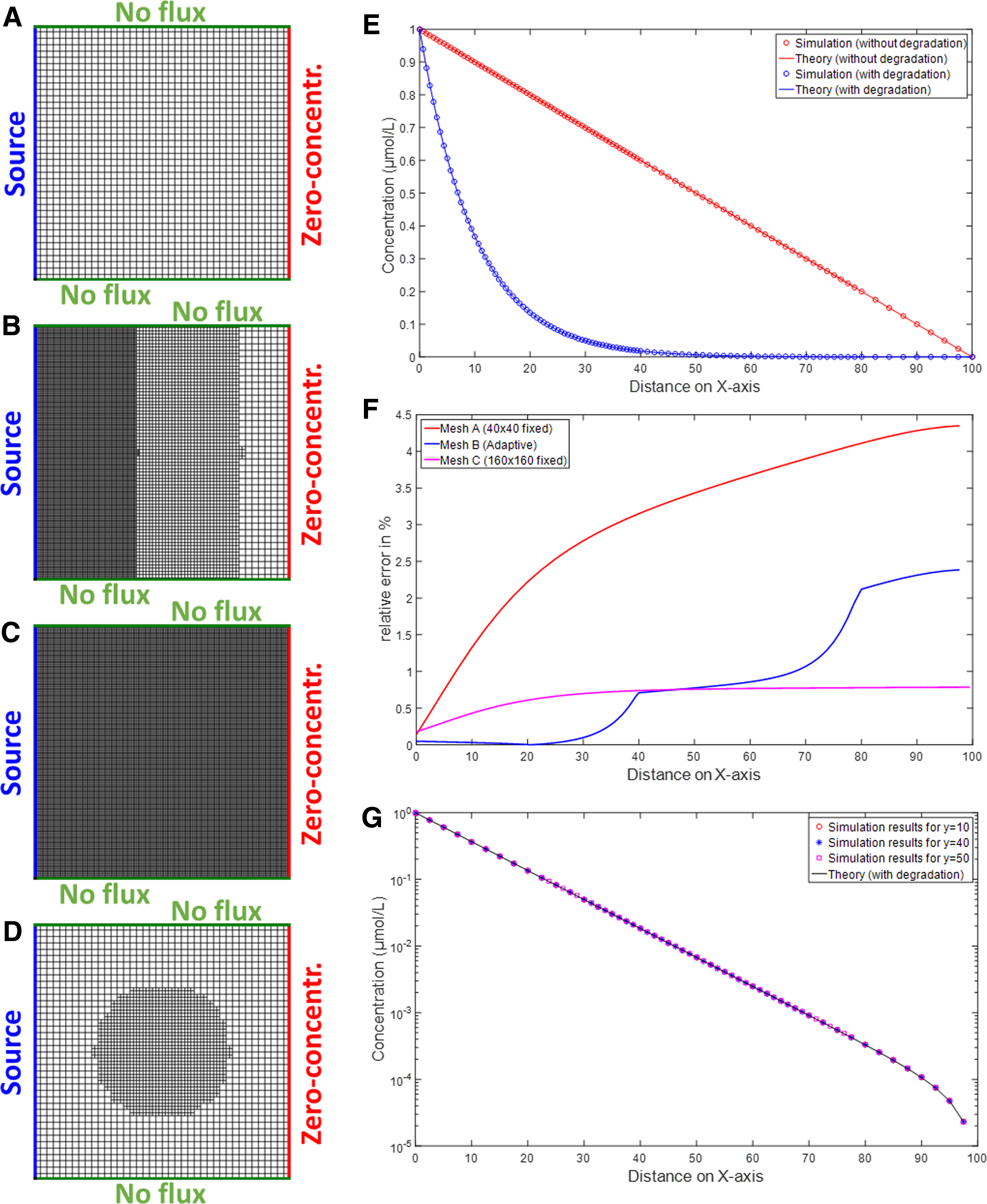
On the left, the four meshes that have been compared. (A) Is a 40 × 40 fixed-size lattice. (B) Is an adaptive lattice based on the lattice (A) refined twice for x between 0 and 40, and once for x between 40 and 80. (C) Is a 160 × 160 fixed-size lattice, that is, the lattice (A) refined twice everywhere. (D) Is an adaptive lattice based on (A) with a circular refinement zone at the center. On the right, simulation results and comparison with the theoretical models for different lattices. Parameters used for the simulation are the following: \documentclass{aastex}\usepackage{amsbsy}\usepackage{amsfonts}\usepackage{amssymb}\usepackage{bm}\usepackage{mathrsfs}\usepackage{pifont}\usepackage{stmaryrd}\usepackage{textcomp}\usepackage{portland, xspace}\usepackage{amsmath, amsxtra}\usepackage{upgreek}\pagestyle{empty}\DeclareMathSizes{10}{9}{7}{6}\begin{document} $$L = 100$$ \end{document} , \documentclass{aastex}\usepackage{amsbsy}\usepackage{amsfonts}\usepackage{amssymb}\usepackage{bm}\usepackage{mathrsfs}\usepackage{pifont}\usepackage{stmaryrd}\usepackage{textcomp}\usepackage{portland, xspace}\usepackage{amsmath, amsxtra}\usepackage{upgreek}\pagestyle{empty}\DeclareMathSizes{10}{9}{7}{6}\begin{document} $$D = 10$$ \end{document} , \documentclass{aastex}\usepackage{amsbsy}\usepackage{amsfonts}\usepackage{amssymb}\usepackage{bm}\usepackage{mathrsfs}\usepackage{pifont}\usepackage{stmaryrd}\usepackage{textcomp}\usepackage{portland, xspace}\usepackage{amsmath, amsxtra}\usepackage{upgreek}\pagestyle{empty}\DeclareMathSizes{10}{9}{7}{6}\begin{document} $$d = 0.1$$ \end{document} , \documentclass{aastex}\usepackage{amsbsy}\usepackage{amsfonts}\usepackage{amssymb}\usepackage{bm}\usepackage{mathrsfs}\usepackage{pifont}\usepackage{stmaryrd}\usepackage{textcomp}\usepackage{portland, xspace}\usepackage{amsmath, amsxtra}\usepackage{upgreek}\pagestyle{empty}\DeclareMathSizes{10}{9}{7}{6}\begin{document} $${ \phi _0} = 0.01$$ \end{document} without degradation, and \documentclass{aastex}\usepackage{amsbsy}\usepackage{amsfonts}\usepackage{amssymb}\usepackage{bm}\usepackage{mathrsfs}\usepackage{pifont}\usepackage{stmaryrd}\usepackage{textcomp}\usepackage{portland, xspace}\usepackage{amsmath, amsxtra}\usepackage{upgreek}\pagestyle{empty}\DeclareMathSizes{10}{9}{7}{6}\begin{document} $${ \phi _0} = 0.1$$ \end{document} with degradation. (E) Corresponds to the simulation of the lattice (B) with and without degradation. (F) Shows a comparison of the relative error between simulations and theoretical curves for lattices (A–C). Finally, (G) is a semilog representation of the result obtained on lattice (D) for three different slices: y = 10 (outside the refinement zone), y = 40 and y = 50 (where the refinement zone is the largest).

4.1.2. Radial diffusion from a central source

In this case, we still consider the same 2D square of length L. The no-flux boundary condition is applied on each border and an incoming flux is applied to the center of the square O. For analytic computation, polar coordinates \documentclass{aastex}\usepackage{amsbsy}\usepackage{amsfonts}\usepackage{amssymb}\usepackage{bm}\usepackage{mathrsfs}\usepackage{pifont}\usepackage{stmaryrd}\usepackage{textcomp}\usepackage{portland, xspace}\usepackage{amsmath, amsxtra}\usepackage{upgreek}\pagestyle{empty}\DeclareMathSizes{10}{9}{7}{6}\begin{document} $$( r , \theta )$$ \end{document} centered on O are preferred. Obviously, concentration is independent of \documentclass{aastex}\usepackage{amsbsy}\usepackage{amsfonts}\usepackage{amssymb}\usepackage{bm}\usepackage{mathrsfs}\usepackage{pifont}\usepackage{stmaryrd}\usepackage{textcomp}\usepackage{portland, xspace}\usepackage{amsmath, amsxtra}\usepackage{upgreek}\pagestyle{empty}\DeclareMathSizes{10}{9}{7}{6}\begin{document} $$\theta$$ \end{document} and, at the steady state, Equation 1 can be rewritten as this: \documentclass{aastex}\usepackage{amsbsy}\usepackage{amsfonts}\usepackage{amssymb}\usepackage{bm}\usepackage{mathrsfs}\usepackage{pifont}\usepackage{stmaryrd}\usepackage{textcomp}\usepackage{portland, xspace}\usepackage{amsmath, amsxtra}\usepackage{upgreek}\pagestyle{empty}\DeclareMathSizes{10}{9}{7}{6}\begin{document} \begin{align*} D \cdot \left( { { \frac { { d^2 } C } { \partial { r^2 } } } + \frac { 1 } { r } \cdot { \frac { dC } { dr } } } \right) - d \cdot C \left( r \right) = 0 \tag { 11 } \end{align*} \end{document}

The analytical solutions of this equation are the modified Bessel functions. More precisely, taking the boundary conditions into account, the solution is: \documentclass{aastex}\usepackage{amsbsy}\usepackage{amsfonts}\usepackage{amssymb}\usepackage{bm}\usepackage{mathrsfs}\usepackage{pifont}\usepackage{stmaryrd}\usepackage{textcomp}\usepackage{portland, xspace}\usepackage{amsmath, amsxtra}\usepackage{upgreek}\pagestyle{empty}\DeclareMathSizes{10}{9}{7}{6}\begin{document} \begin{align*} C \left( r \right) = { \phi _0 } \cdot { K_0 } \left( { \sqrt { \frac { d } { D } } \cdot r } \right) \tag { 12 } \end{align*} \end{document}

Table 2.

Description of the Lattices for the Benchmark

	Description				Model		CPU time (seconds)
		Refinement					Spectre		NGSpice
Lattice number	Initial lattice	n = 1	n = 2	n = 3	Number of nodes	Number of meshes	SSA	TC	SSA	TC
1	40 × 40				1,681	1,600	1.5	1.7	1.4	9.4
2	40 × 40	25			2,779	2,656	2.1	4.6	3.1	20.1
3	20 × 20				441	400	0.6	0.5	0.4	2.4
4	80 × 80				6,561	6,400	5.5	8.7	11.3	59.1
5	40 × 40	100			6,561	6,400	5.3	9.3	11.0	57.4
6	40 × 40	100	50	25	36,991	36,514	111.0	202.0	323.0	996.0
7	100 × 100				10,201	10,000	14.5	18.7	20.5	80.8
8	25 × 25	50	25		3,997	3,844	3.1	6.6	5.6	29.9
9	25 × 25	30	15		1,969	1,855	1.29	3.4	2.2	13.2
10	25 × 25	20	5		1,109	1,024	0.7	1.1	1.3	6.3
11	25 × 25		50		8,647	8,446	7.7	15.4	19.0	74.4

Description of the lattices for the benchmark. For all of them, the initial (unrefined) lattice, the refinement zones, the number of nodes and elementary meshes, as well as the simulation time for SSA and TC simulations are given, both for NGSpice and Spectre. Values in the refinement column are the diameter of the refinement zone (centered on O). Computation time with Spectre and NGSPICE have been obtained on a 12-core 2.6-GHz CPU with 40 Go of RAM. TC simulations are performed with a built-in adaptive time step algorithm configured to simulate over 100 seconds with a minimal time step of 5 seconds.

SSA, steady-state analysis; TC, time-course.

When comparing the steady state values of the nodes for the different layouts, it appears that they are very similar however far they are from the source. For this reason, we choose to show only the close vicinity of the source in the results. Mesh No. 4 and Mesh No. 5 are equivalent, but have been obtained in two different ways: one directly, the other using a refinement on the whole area. Thus, even if their netlists are different, the ODE set generated by model compilation, the simulation results are identical. This indicates that the refinement has been well considered into the model of the elemental mesh. Moreover, we can see that most of the results obtained with different lattices overlap and are in accordance with the theoretical model (Fig. 4A).

FIG. 4.

Simulation results of the steady-state concentration on nodes according to their distance toward the source for different lattice layouts, and comparison with the analytic solution (A). A focus on the central node and the effect of the discretization is given in (B). The relative error between simulation results and the analytic solution as a function of the lattice is represented in (C). Simulation results are obtained with the following parameters: \documentclass{aastex}\usepackage{amsbsy}\usepackage{amsfonts}\usepackage{amssymb}\usepackage{bm}\usepackage{mathrsfs}\usepackage{pifont}\usepackage{stmaryrd}\usepackage{textcomp}\usepackage{portland, xspace}\usepackage{amsmath, amsxtra}\usepackage{upgreek}\pagestyle{empty}\DeclareMathSizes{10}{9}{7}{6}\begin{document} $$L = 100$$ \end{document} , \documentclass{aastex}\usepackage{amsbsy}\usepackage{amsfonts}\usepackage{amssymb}\usepackage{bm}\usepackage{mathrsfs}\usepackage{pifont}\usepackage{stmaryrd}\usepackage{textcomp}\usepackage{portland, xspace}\usepackage{amsmath, amsxtra}\usepackage{upgreek}\pagestyle{empty}\DeclareMathSizes{10}{9}{7}{6}\begin{document} $$D = 10$$ \end{document} , \documentclass{aastex}\usepackage{amsbsy}\usepackage{amsfonts}\usepackage{amssymb}\usepackage{bm}\usepackage{mathrsfs}\usepackage{pifont}\usepackage{stmaryrd}\usepackage{textcomp}\usepackage{portland, xspace}\usepackage{amsmath, amsxtra}\usepackage{upgreek}\pagestyle{empty}\DeclareMathSizes{10}{9}{7}{6}\begin{document} $$d = 0.1$$ \end{document} and \documentclass{aastex}\usepackage{amsbsy}\usepackage{amsfonts}\usepackage{amssymb}\usepackage{bm}\usepackage{mathrsfs}\usepackage{pifont}\usepackage{stmaryrd}\usepackage{textcomp}\usepackage{portland, xspace}\usepackage{amsmath, amsxtra}\usepackage{upgreek}\pagestyle{empty}\DeclareMathSizes{10}{9}{7}{6}\begin{document} $${ \phi _0} = 0.4$$ \end{document} . Simulation results are fitted with the Bessel function \documentclass{aastex}\usepackage{amsbsy}\usepackage{amsfonts}\usepackage{amssymb}\usepackage{bm}\usepackage{mathrsfs}\usepackage{pifont}\usepackage{stmaryrd}\usepackage{textcomp}\usepackage{portland, xspace}\usepackage{amsmath, amsxtra}\usepackage{upgreek}\pagestyle{empty}\DeclareMathSizes{10}{9}{7}{6}\begin{document} $$C \left( r \right) = 0.4 \cdot {K_0} \cdot\left( { \sqrt {0.01} \cdot r} \right)$$ \end{document} or \documentclass{aastex}\usepackage{amsbsy}\usepackage{amsfonts}\usepackage{amssymb}\usepackage{bm}\usepackage{mathrsfs}\usepackage{pifont}\usepackage{stmaryrd}\usepackage{textcomp}\usepackage{portland, xspace}\usepackage{amsmath, amsxtra}\usepackage{upgreek}\pagestyle{empty}\DeclareMathSizes{10}{9}{7}{6}\begin{document} $${K_0} \cdot \left( { \sqrt {0.1} \cdot r} \right)$$ \end{document} .

However, we note a significant difference at the source. This difference is an effect of discretization. It is illustrated on Figure 4B. When PDEs are solved with a finite difference model, the value computed for the concentration at a given node is the integral of the concentration on a surface around this node. Obviously, the size of this surface depends on the mesh refinement around the given node. The blue curve on Figure 4B corresponds to the theoretical model. Consider now the center of the lattice. For large meshes (typ. Lattice No. 3), the integration surface is larger and the value at the central point is lower. For thinner meshes (typ. Lattice No. 5), the integration surface decreases, and the value at the central point increases. This phenomenon is amplified around the center, where the gradient of concentration is higher than near the borders. The difference between observed curves shows that some lattices used for simulation are not refined enough to produce accurate results near the center (Fig. 4B). Conversely, if the area of interest is far from the center, all the lattices give equivalent results.

Obviously, the drawback of a highly refined grid is the increased number of nodes and meshes and thus an increase in the computation time, as illustrated on Figure 5.

FIG. 5.

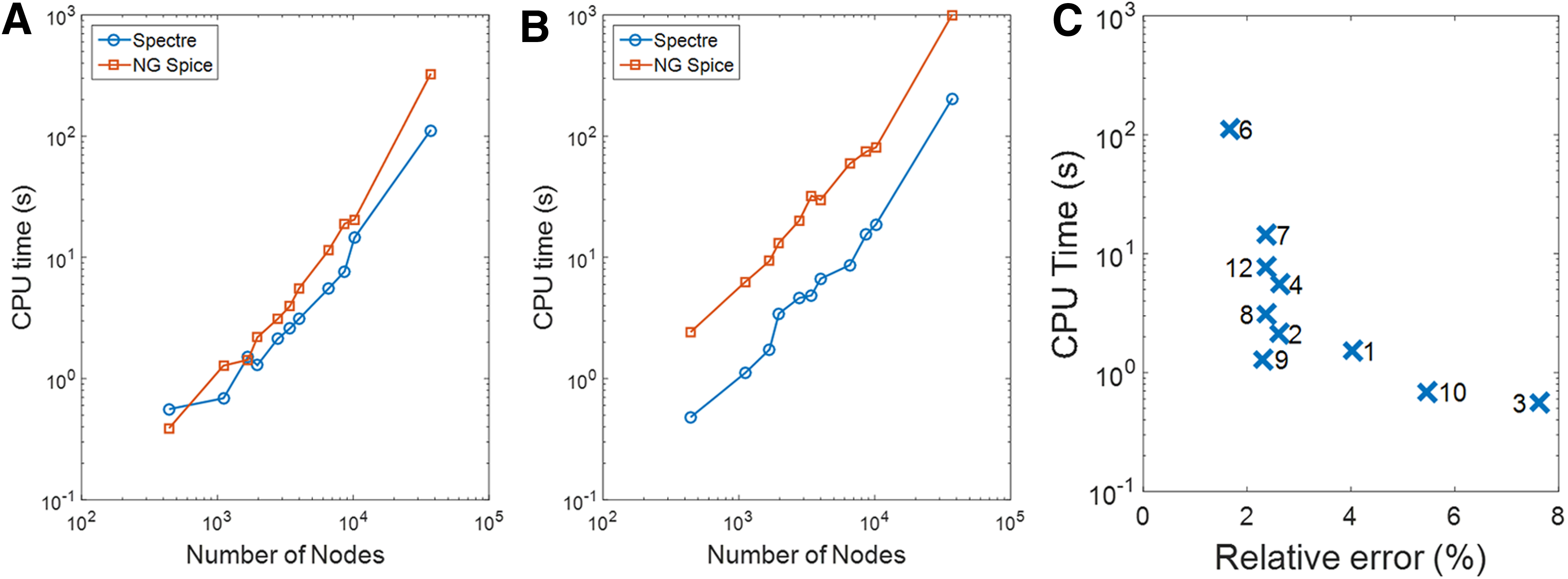
Computation time for the different lattices. (A) Gives a comparison of the evolution of the computation time as a function of the number of nodes for a steady-state simulation with Spectre and NGSpice. (B) Is the same comparison for a time course analysis. Finally, (C) gives the position of the different lattices on maximal relative error versus computation time map for a steady-state simulation with Spectre. Simulation have been carried out on a 12-core 2.6-GHz CPU with 40 Go of RAM.

4.2. Applications

4.2.1. Basu's system

Our tool is now applied on an actual biological system. The first example is a biological pattern formation system developed by Basu et al. (2005). The system allows the formation of green fluorescent protein (GFP) patterns in a closed space by making use of two populations of cells: the senders and the receivers. The senders communicate with the receivers by synthesizing and isotopically emitting a small molecule able to diffuse and enter cells, acyl-homoserine lactone (AHL). Receivers react to intermediate concentrations of AHL. Upon receiving the correct amount of AHL, receivers produce GFP that is the output in this system. In practice, a Petri dish is covered with receiver cells and one or many groups of senders are laid on specific spots.

This system is modeled as following. First, we define a diffusion layer for AHL using our tool. Second, we model the behavior of the group of senders as continuous AHL sources (constant current sources in our electronic analogy). Finally, we instantiate at each node, a model of receiver. This model has been established in a previous work (Rosati et al., 2016) and translated in Verilog-A and SPICE. To simplify the model, we assume that the cell membranes are fully permeable to AHL. Thus, the concentrations of AHL inside and outside the receiver are equal. However, it should be noticed that there are no technical obstacles related to the integration of more sophisticated models for the membrane transport of AHL inside the cell.

Two configurations are tested: one with only one group of sender cells in the middle (Fig. 6A) and another one with three groups of sender cells (Fig. 6B). For both configurations, we use as a base lattice, a square of 100 × 100 units with 40 divisions per axis. In the first configuration, we added one circular refinement zone with a radius of 25 centered at the sender cell (x = 50 and y = 50), with a refinement coefficient of 1 (Fig. 6C). The concentration of AHL and GFP according to space at the steady state can be observed on Figure 6E and F, with the sender cell represented as a red dot. Transient evolution of AHL and GFP concentrations are monitored at three nodes, located on the diagonal from the center toward the lower left corner (Fig. 6I). As AHL diffuses from its centered source, the peak of GFP propagates from the center toward the borders of the lattice, as it first appears at the node (40,40) in black and then at the node (37.5,37.5), where it stops as expected. In the second configuration, we added three circular refinement zones with a radius of 35 centered at the sender cells, namely coordinates (50,35), (35,60), and (65,60), with a refinement coefficient of 2 (Fig. 6D).

FIG. 6.

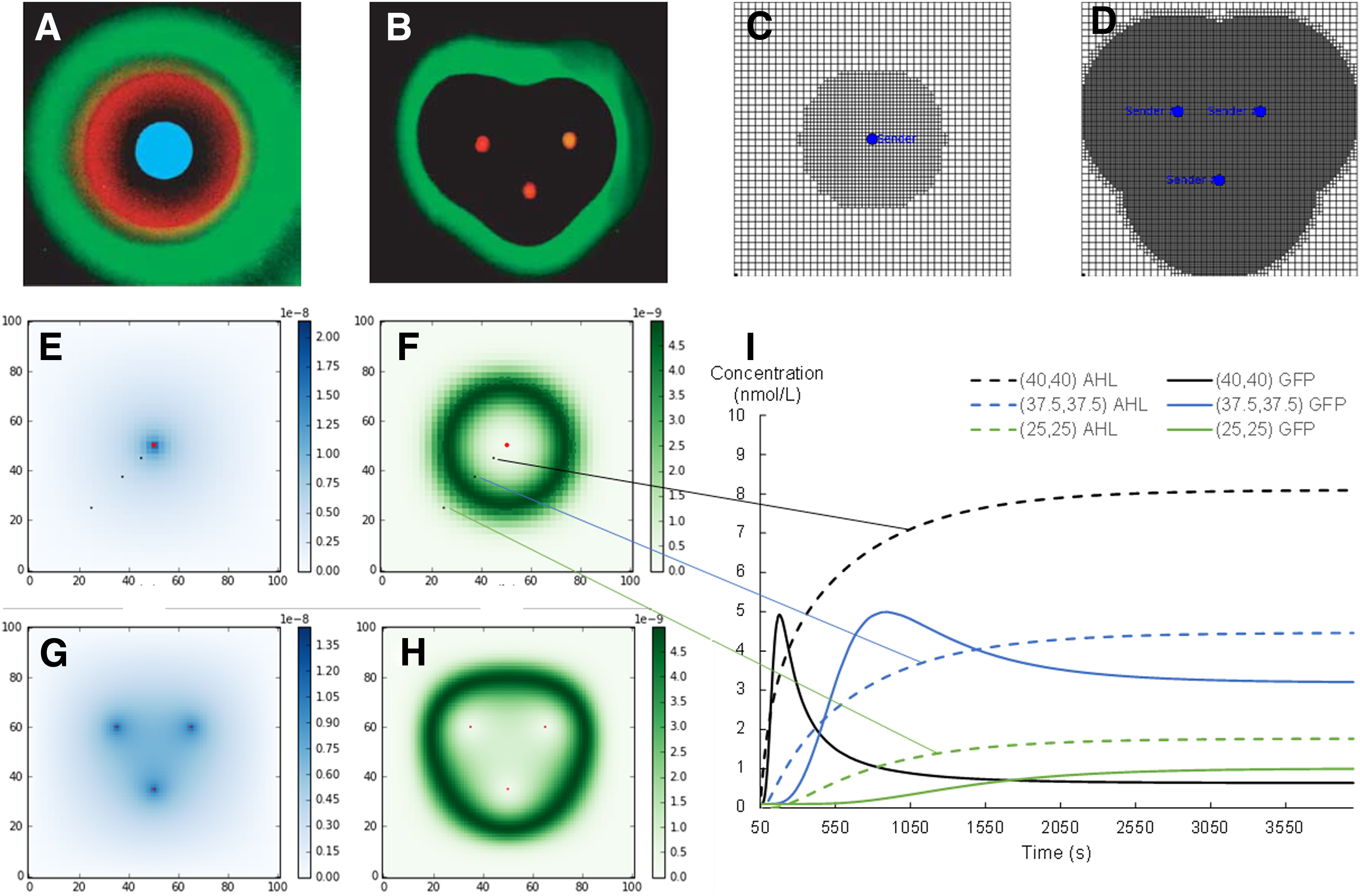
Simulation of the band-pass system with one or three sender cells. (A and B) correspond to experimental results extracted from Basu et al. (2005). (C and D) are the lattices used for resp. the configuration with one sender and the configuration with three senders. (E and G) are the simulated map representing the concentration of AHL at the steady state for both configurations. (F and H) are the simulated map representing the concentration of GFP at the steady state for both configurations. Finally, (I) is a representation of the temporal evolution of AHL and GFP at three different points: (40,40), (37.5,37.5), and (25,25) for the configuration with a single sender. AHL, acyl-homoserine lactone; GFP, green fluorescent protein.

Steady-state spatial map of AHL and GFP for this configuration are also given in Figure 6G and H. Obtained simulation results are in agreement with the experimental results provided by Basu et al. (2005) and reproduced on Figure 6A and B. Indeed, our simulation successfully obtains a ring of fluorescent cells around the emitting node, or a triangular ring around the three emitting cells in the second case. For both configurations, the number of receiver cell models, of nodes and of meshes instantiated as well as the required computation time are given in Table 3. They correspond to a steady-state (operating point) simulation.

Table 3.

Comparison of the Number of Elementary Meshes, Number of Receiver Models, and the Total Number of Nodes (Nodes of the Lattice+Nodes Inside Each Receiver Model) and the CPU Time for a Steady-State Simulation with Spectre on a 12-core 2.6-GHz CPU with 40 Go of RAM

	Model with a single sender	Model with 3 senders
Number of meshes	2,656	19,798
Number of instances of receiver cell models	2,779	20,119
Total number of instantiated nodes	19,453	140,833
CPU time (seconds)	3.6	113.0

4.2.2. Simplified prey–predator system

Prey–predator ecosystems are composed of two kinds of organisms whose activity depends on each other (e.g., rabbits and foxes). Recently, artificial prey–predator ecosystems have been demonstrated with artificially reprogrammed cells (Balagaddé et al., 2008; Fujii and Rondelez, 2013). In existing models, spatiality, which may play a key role in the process, is not taken into account. In this work, focus is put on the diffusion process. Thus, the model of the prey and the predator will be simplified at most.

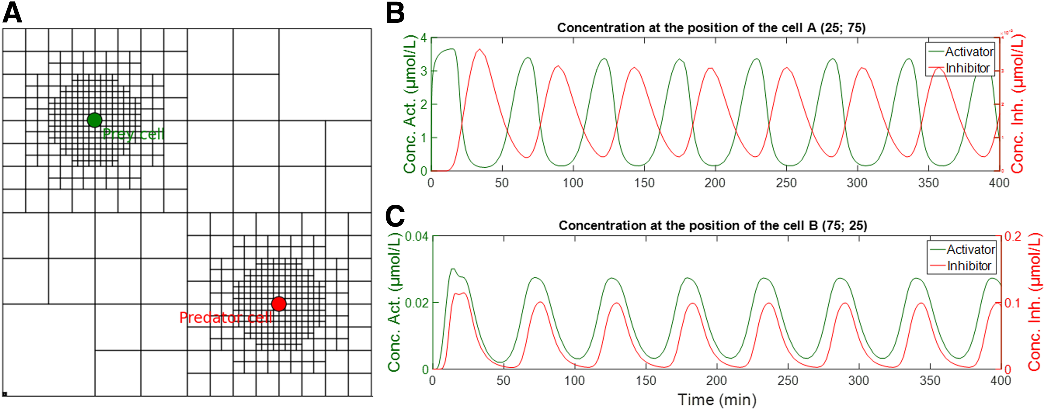
The modeled system is composed of two cells. In the cell A, which mimics the prey, a gene synthesizes a transcription factor X that activates a gene inside the cell B, which mimics the predator. In the cell B, the activated gene synthesizes in turn an inhibitor Y for the gene in the cell A. By this way, when the concentration of X increases, production of Y increases, which in turn reduces the concentration of X. Under the appropriate conditions, this system should oscillate.

Results obtained with our simulator are given on Figure 7. Again, we use as a base lattice, a square of 100 × 100 units with four divisions per axis. The positions of cells A and B are (25,75) and (75,25), respectively. Two circular refinement zones with a radius of 10 and a degree of refinement of 4 are built around each cell. The obtained lattice is represented on Figure 7A. Two diffusion layers are defined, one for X and one for Y. Both layers are independent except on nodes (25,75) and (75,25), where they are connected through two external models, one for the behavior of the cell A and one for the behavior of the cell B. Models used for cells A and B correspond to simple regulation using Hill's equations (Konkoli, 2011). Thus, in cell A, the transcription of DNA and the translation of mRNA into X are given by: \documentclass{aastex}\usepackage{amsbsy}\usepackage{amsfonts}\usepackage{amssymb}\usepackage{bm}\usepackage{mathrsfs}\usepackage{pifont}\usepackage{stmaryrd}\usepackage{textcomp}\usepackage{portland, xspace}\usepackage{amsmath, amsxtra}\usepackage{upgreek}\pagestyle{empty}\DeclareMathSizes{10}{9}{7}{6}\begin{document} \begin{align*} { \frac { d \left[ { mRN { A_A } } \right] } { dt } } = { K_ { TR } } \cdot { \frac { { K_A } ^ { { n_A } } } { { K_A } ^ { { n_A } } + { { \left[ Y \right] } ^ { { n_A } } } } } - d \cdot \left[ { mRN { A_A } } \right] \tag { 13 } \end{align*} \end{document} \documentclass{aastex}\usepackage{amsbsy}\usepackage{amsfonts}\usepackage{amssymb}\usepackage{bm}\usepackage{mathrsfs}\usepackage{pifont}\usepackage{stmaryrd}\usepackage{textcomp}\usepackage{portland, xspace}\usepackage{amsmath, amsxtra}\usepackage{upgreek}\pagestyle{empty}\DeclareMathSizes{10}{9}{7}{6}\begin{document} \begin{align*} { \frac { d \left[ X \right] } { dt } } = { K_ { TL } } \cdot \left[ { mRN { A_A } } \right] - d \cdot \left[ X \right] \tag { 14 } \end{align*} \end{document}

FIG. 7.

(A) Mesh generated for the simulation of the simplified prey–predator system. (B, C) Simulation results of the transient evolution of the concentration of activator (X) and inhibitor (Y) at the position of cells, respectively, at the cell A and at the cell B. Parameters used for the simulation are the following: \documentclass{aastex}\usepackage{amsbsy}\usepackage{amsfonts}\usepackage{amssymb}\usepackage{bm}\usepackage{mathrsfs}\usepackage{pifont}\usepackage{stmaryrd}\usepackage{textcomp}\usepackage{portland, xspace}\usepackage{amsmath, amsxtra}\usepackage{upgreek}\pagestyle{empty}\DeclareMathSizes{10}{9}{7}{6}\begin{document} $$D = 2$$ \end{document} m²/s, \documentclass{aastex}\usepackage{amsbsy}\usepackage{amsfonts}\usepackage{amssymb}\usepackage{bm}\usepackage{mathrsfs}\usepackage{pifont}\usepackage{stmaryrd}\usepackage{textcomp}\usepackage{portland, xspace}\usepackage{amsmath, amsxtra}\usepackage{upgreek}\pagestyle{empty}\DeclareMathSizes{10}{9}{7}{6}\begin{document} $$d = {10^{ - 6}}$$ \end{document} /min for the diffusion, \documentclass{aastex}\usepackage{amsbsy}\usepackage{amsfonts}\usepackage{amssymb}\usepackage{bm}\usepackage{mathrsfs}\usepackage{pifont}\usepackage{stmaryrd}\usepackage{textcomp}\usepackage{portland, xspace}\usepackage{amsmath, amsxtra}\usepackage{upgreek}\pagestyle{empty}\DeclareMathSizes{10}{9}{7}{6}\begin{document} $${K_{{ \rm{TR}}}} = {10^{ - 3}}$$ \end{document} μmol/(L·min), \documentclass{aastex}\usepackage{amsbsy}\usepackage{amsfonts}\usepackage{amssymb}\usepackage{bm}\usepackage{mathrsfs}\usepackage{pifont}\usepackage{stmaryrd}\usepackage{textcomp}\usepackage{portland, xspace}\usepackage{amsmath, amsxtra}\usepackage{upgreek}\pagestyle{empty}\DeclareMathSizes{10}{9}{7}{6}\begin{document} $${K_{{ \rm{TL}}}} = {10^{ - 2}}$$ \end{document} /min for the transcription rate and translation rate inside the cells, \documentclass{aastex}\usepackage{amsbsy}\usepackage{amsfonts}\usepackage{amssymb}\usepackage{bm}\usepackage{mathrsfs}\usepackage{pifont}\usepackage{stmaryrd}\usepackage{textcomp}\usepackage{portland, xspace}\usepackage{amsmath, amsxtra}\usepackage{upgreek}\pagestyle{empty}\DeclareMathSizes{10}{9}{7}{6}\begin{document} $${K_{ \rm{R}}} = {10^{ - 6}}$$ \end{document} mol/L and \documentclass{aastex}\usepackage{amsbsy}\usepackage{amsfonts}\usepackage{amssymb}\usepackage{bm}\usepackage{mathrsfs}\usepackage{pifont}\usepackage{stmaryrd}\usepackage{textcomp}\usepackage{portland, xspace}\usepackage{amsmath, amsxtra}\usepackage{upgreek}\pagestyle{empty}\DeclareMathSizes{10}{9}{7}{6}\begin{document} $${n_{ \rm{R}}} = 3$$ \end{document} for Hill's equation used to model the transcription in the cell A, and \documentclass{aastex}\usepackage{amsbsy}\usepackage{amsfonts}\usepackage{amssymb}\usepackage{bm}\usepackage{mathrsfs}\usepackage{pifont}\usepackage{stmaryrd}\usepackage{textcomp}\usepackage{portland, xspace}\usepackage{amsmath, amsxtra}\usepackage{upgreek}\pagestyle{empty}\DeclareMathSizes{10}{9}{7}{6}\begin{document} $${K_{ \rm{A}}} = {10^{ - 4}}$$ \end{document} mol/L and \documentclass{aastex}\usepackage{amsbsy}\usepackage{amsfonts}\usepackage{amssymb}\usepackage{bm}\usepackage{mathrsfs}\usepackage{pifont}\usepackage{stmaryrd}\usepackage{textcomp}\usepackage{portland, xspace}\usepackage{amsmath, amsxtra}\usepackage{upgreek}\pagestyle{empty}\DeclareMathSizes{10}{9}{7}{6}\begin{document} $${n_{ \rm{R}}} = 3$$ \end{document} for Hill's equation used to model the transcription in the cell B.

By the same way, in cell B, the transcription of DNA and the translation of mRNA into Y are given by: \documentclass{aastex}\usepackage{amsbsy}\usepackage{amsfonts}\usepackage{amssymb}\usepackage{bm}\usepackage{mathrsfs}\usepackage{pifont}\usepackage{stmaryrd}\usepackage{textcomp}\usepackage{portland, xspace}\usepackage{amsmath, amsxtra}\usepackage{upgreek}\pagestyle{empty}\DeclareMathSizes{10}{9}{7}{6}\begin{document} \begin{align*} { \frac { d \left[ { mRN { A_B } } \right] } { dt } } = { K_ { TR } } \cdot { \frac { { { \left[ X \right] } ^ { { n_R } } } } { { K_R } ^ { { n_R } } + { { \left[ X \right] } ^ { { n_R } } } } } - d \cdot \left[ { mRN { A_B } } \right] \tag { 15 } \end{align*} \end{document} \documentclass{aastex}\usepackage{amsbsy}\usepackage{amsfonts}\usepackage{amssymb}\usepackage{bm}\usepackage{mathrsfs}\usepackage{pifont}\usepackage{stmaryrd}\usepackage{textcomp}\usepackage{portland, xspace}\usepackage{amsmath, amsxtra}\usepackage{upgreek}\pagestyle{empty}\DeclareMathSizes{10}{9}{7}{6}\begin{document} \begin{align*} { \frac { d \left[ Y \right] } { dt } } = { K_ { TL } } \cdot \left[ { mRN { A_B } } \right] - d \cdot \left[ Y \right] \tag { 16 } \end{align*} \end{document}

Again, to simplify the model, we consider that cell membranes are permeable to both the activator and the inhibitor, such that the concentrations inside and outside the cell are equal. As expected from Balagaddé et al. (2008), three different dynamics can be found depending on the parameters of the system as well as the distance between cells: coexistence, extinction, or oscillations. Oscillatory behavior is represented on Figure 7B and C.

5. Discussion

The previous section highlighted the validity of our approach and showed two application examples. In this section, performances of our approach are discussed. As mentioned in the introduction, Virtual Cell and COMSOL can be considered as the major alternatives to our tool. On the one hand, Virtual Cell has an intuitive Graphical User Interface (GUI) that can be used to define the geometry of the problem (which can be imported from actual segmented microscopy images) and biological reactions. Several solvers are available, including deterministic and stochastic simulation for 0D to 3D problems. It was tested on the aforementioned benchmarks and led to results comparable to those obtained with our tool.

Nevertheless, Virtual Cell performs only transient simulations. Static simulation results have been obtained by performing a transient simulation up to the steady state, which is time consuming. Computations are not done locally on the computer, but are dispatched and executed on a remote server. Thus, comparison of computation time is not very relevant. Results given in Table 4 correspond to wall-clock computation time and are independent of the computer on which they are performed. Virtual Cell also uses a lattice to solve PDE, but the mesh size is fixed. Thus, to obtain a 1 mm spatial resolution at the center, it is necessary to have a 1 mm length mesh on the whole surface, which leads to 10,201 nodes. It is between three and four times more than the number of nodes required to obtain the same spatial resolution near the source and the same accuracy with an adaptive lattice. Finally, the other limitation of Virtual Cell is the difficulty to couple biological models with models from other domains of physics. It may be possible in several cases, but it requires a translation of physical problems into an equivalent biochemical problem.

Table 4.

Comparison of the Features and the Performances of Virtual Cell, COMSOL, and Our Approach (Both with Spectre and NGSpice)

	COMSOL	Virtual cell	Spectre	NGSPICE
Mesher	Triangle	Rectangular	Rectangular	Rectangular
	Adaptive mesh	Fixed	Adaptive	Adaptive
	Driven by physics		Defined by user	Defined by user
Discretization scheme	Finite elements (various scheme)	Finite differences	Finite differences	Finite differences
Multiphysics interface	Yes	Not straightforward	Yes, using Kirchhoff-based equivalent circuits and hardware description language	Yes, using Kirchhoff-based equivalent circuits and hardware description language
Multiphysics interface	Coupling with other COMSOL module	Not straightforward
Simulation type	Deterministic	Deterministic or stochastic	Deterministic	Deterministic
Simulation type	Steady state, transient, parametric	Transient	Steady state, transient, parametric, frequency analysis, noise analysis	Steady state, transient, parametric, frequency analysis, noise analysis
Scripting for the development of complex testbenchs	Yes, with MATLAB	No	Yes, with SPICE simulation control directives	Yes, with SPICE simulation control directives
Software type	Commercial	Freeware	Open-source model generator commercial simulator	Fully open source
Computation time in steady state	<1 seconds for a 1858-nodes model	No steady state simulation	14.5 seconds for a regular 100 × 100 mesh.	20.5 seconds for a regular 100 × 100 mesh.
Computation time in steady state	<1 seconds for a 1858-nodes model		1.29 seconds for a 1969-node adaptive mesh.	2.19 seconds for a 1969-node adaptive mesh.
Computation time in transient	19 seconds for a 1858-nodes model and 20 time steps	140 seconds for a 10,201-nodes model and 20 time steps	18.7 seconds for a regular 100 × 100 mesh and 20 time steps	80.8 seconds for a regular 100 × 100 mesh and 20 time steps
Computation time in transient	19 seconds for a 1858-nodes model and 20 time steps	140 seconds for a 10,201-nodes model and 20 time steps	3.44 seconds for a 1969-node adaptive mesh and 20 time steps	13.18 seconds for a 1969-node adaptive mesh and 20 time steps

On the other hand, COMSOL is a software dedicated to the simulation of multiphysics systems. It provides modules dedicated to the diffusion of chemical species and to the engineering of reactions that can be coupled together and with other modules from other domains of physics. It has already been used for the study of biochemical systems (Dreij et al., 2011; Vollmer et al., 2013). The PDE solver as well as the mesher implemented in COMSOL are more sophisticated than that proposed in our approach. The adaptive lattice can be computed automatically by COMSOL according to the geometry and the problem itself (detection of hot spots to determine automatically the refinement zones), whereas it has to be defined by the user in our case. The definition of the geometry and the diffusion equations are simplified by a GUI. Contrariwise, the definition of the reactions is less intuitive. Importing existing biological models or integrating complex reaction models is painful. The PDE resolution algorithms are various and optimized for a multicore implementation, which leads to low computation times as shown in Table 4. Most common simulation types (i.e., static, dynamic, parametric) are available and COMSOL can be coupled with MATLAB to build an enhanced test bench. Unfortunately, COMSOL is an expensive commercial tool which limits its application range, especially in the academic field.

Compared with them, our approach offers a solution that positions itself as a good tradeoff between accuracy and computation speed, relies on tools that have proved their efficiency for years (to simulate systems as complex as 1-billion transistors microprocessors), and offers a direct coupling with other domains of physics through the generalized Kirchhoff's laws. Comparison on several features among our approach, COMSOL, and Virtual Cell are given in Table 4. Comparison between simulation results and computation time is not straightforward because of the different ways simulators are implemented and the different computers on which they were performed. Benchmark used for comparison is the one described in Section 4.1.2., that is, a 100 × 100 square with a source at (50,50) and no-flux boundary conditions. The spatial resolution near the source should be at least 1 mm.

As Virtual Cell does not propose an adaptive mesher, a 101 × 101 lattice is used to discretize the whole surface. With COMSOL, an adaptive 1858-node mesh is generated so that the smallest elements are less than 1 mm at the center. Finally, with our tools, 11 different lattices have been tested (Table 2). Reduction in the number of nodes obviously degrades the quality of the results, but, in counterpart, drastically reduces the computation time. Results retained for the comparison are those from Mesh No. 7 (regular lattice) and Mesh No. 9 (adaptive lattice), which can be considered as a good tradeoff between computation time and accuracy (Fig. 5). Moreover, we compared the performances of Spectre and NGSPICE for our approach. The commercial simulator has better performance than the open-source one when the number of nodes exceeds 2000 (Fig. 5). This is even more marked on transient simulation. This is probably due to the multicore feature proposed by Spectre, and which is not yet supported by NGSpice.

As a conclusion, compared with existing approaches, our simulator exhibits four main advantages: (1) it is based on a very simple algorithm for the discretization of space, which facilitates the description of the diffusion phenomena with simple compact models; (2) it provides a direct coupling between the diffusion model of molecules, models of biological systems that play a role inside the diffusion medium and models from other domains of physics; (3) it uses a SPICE simulation core, which has proven its efficiency for years, especially for systems with a high number of differential equations and which will be improved in the near future to face the new challenges of microelectronics; and (4) it is open source. With these features, it is a very powerful tool for the simulation and the virtual prototyping of biological systems inside cells or involving diverse types of cells that communicate between them through chemical messengers. For instance, it can be coupled with evolutionary algorithms to explore novel solutions that exploit cells' consortia in synthetic biology or to gain a level of complexity in the modeling of biological systems.

Although the model is simplified due to the implemented discretization algorithm (in comparison with COMSOL models for instance), the simulation of a complete model can be very time consuming, especially when the number of species increases. Considering the properties of the equations to solve, the deployment of Graphical Processor Unit (GPU) could provide a solution to speed-up the computation. Recent versions of GPU-optimized open-source SPICE simulator have been released (Keiter et al., 2014; Lannutti, 2014) and their coupling with our tool is currently under investigation. Another outlook of this work is to improve the elementary model of the mesh and the way several mesh layers can be interconnected for systems with multiple diffusing species. Up to now, the elementary model is based on a finite difference algorithm, which is easy to implement, but may introduce artifacts and convergence issues. The benefit of the development of an elementary mesh model based on more sophisticated discretization scheme (e.g., finite element) has to be investigated. Along the same line, when multiple mesh layers are implemented (e.g., in the simplified prey-predator example), refinement is applied on each layer to facilitate the interconnection between them. Applying specific refinement on each layer would make the generation of the netlist more complex but, on the other hand, would reduce the number of nodes in the model and speed-up the computation.

6. Conclusion

In this article, an innovative way to simulate space-dependent biological systems is presented. The tools are based on the analogy that exists between biochemical reaction and molecule diffusion on the one hand, and electronic and thermal systems on the other hand. It combines an electronic circuit simulator (SPICE) and a mesher that is adapted to deal with biological systems. The validity of the tools has been first demonstrated on very simple use cases, for which an analytical solution exists, then applied on actual biological systems and compared with experimental data extracted from the literature. Moreover, performances of our tool approach have been evaluated in comparison with two other widespread software (COMSOL and Virtual Cell). Again, we highlighted that our tool gathered interesting features (open-source, robust simulation heart, optimized resource usage, direct coupling with other domains of physics) that are not found together in the other studied tools. The current version of the tool is functional and models can be constructed through a Python script that is available as Supplementary Material. A GUI as well as other improvements, which have been discussed in the previous section, are still under investigation and development.

Footnotes

Author Disclosure Statement

No competing financial interests exist.

References

Amar

, Bernot

, and Norris

2004. HSIM: A simulation programme to study large assemblies of proteins. J. Biol. Phys. Chem., 4, 79–84.

Arifin

D.Y.

, Lee

L.Y.

, and Wang

C.-W.

2006. Mathematical modeling and simulation of drug release from microspheres: Implications to drug delivery systems. Adv. Drug Deliv. Rev., 58, 1274–1325.

Balagaddé

F.K.

, Song

, Ozaki

, et al. 2008. A synthetic Escherichia coli predator-prey ecosystem. Mol. Syst. Biol., 4, 187.

Basu

, Gerchman

, Collins

C.H.

, et al. 2005. A synthetic multicellular system for programmed pattern formation. Nature, 434, 1130–1134.

Blundell

, and Blundell

K.M.

2010. Concepts in Thermal Physics. Oxford University Press, United Kingdom.

Butterworth

, Jardine

, Raymond

, et al. 2013. JSim, an open-source modeling system for data analysis. F1000Res, 2, 288.

Calzone

, Fagès

, and Soliman

2006. BIOCHAM: An environment for modeling biological systems and formalizing experimental knowledge. Bioinformatics, 22, 1805–1807.

Digele

, Lindenkreuz

, and Kasper

1997. Fully coupled dynamic electro-thermal simulation. IEEE Trans. Very Large Scale Integration Syst., 5, 250–257.

Dreij

, Chaudhry

Q.A.

, Jernström

, et al. 2011. A method for efficient calculation of diffusion and reactions of lipophilic compounds in complex cell geometry. PLoS One, 6, e23128.

10.

Ermentrout

G.B.

, and Edelstein-Keshet

1993. Cellular automata approaches to biological modeling. J. Theor. Biol., 160, 97–133.

11.

Evans

G.A.

, Blackledge

J.M.

, Jonathan

, et al. 2000. Numerical Methods for Partial Differential Equations. Springer, London, United Kingdom.

12.

Fick

1855. On liquid diffusion. Philos. Mag., 10, 30–39.

13.

Fujii

, and Rondelez

2013. Predator–prey molecular ecosystems. ACS Nano, 7, 27–34.

14.

Garci

, Kammerer

J.-B.

, and Hebrard

2014. Compact modeling and electro-thermal simulation of hot carriers effect in analog circuits, pp 125–128. In 2014 IEEE 12th International New Circuits and Systems Conference (NEWCAS). Montreal, Canada.

15.

Gendrault

, Madec

, Lallement

, et al. 2014. Modeling biology with HDL languages: A first step toward a genetic design automation tool inspired from microelectronics. IEEE Trans. Biomed. Eng., 61, 1231–1240.

16.

Goldbeter

, Dupont

, and Berridge

M.J.

1990. Minimal model for signal-induced Ca2+ oscillations and for their frequency encoding through protein phosphorylation. Proc. Natl Acad. Sci. U. S. A., 87, 1461–1465.

17.

Haiech

, Gendrault

, and Kilhoffer

2014. A general framework improving teaching ligand binding to a macromolecule. Biochim. Biophys. Acta, 1843, 2348–2355.

18.

Hecht

2012. New development in freefem++. J. Numerical Math., 20, 251–266.

19.

Hoops

, Sahle

, Gauges

, et al. 2006. COPASI—A complex pathway simulator. Bioinformatics, 22, 3067–3074.

20.

Hucka

2003. The systems biology markup language (SBML): A medium for representation and exchange of biochemical network models. Bioinformatics, 19, 524–531.

21.

Keiter

, Mei

, Russo

, et al. 2014. Xyce parallel electronic simulator users guide, version 6.1. No. SAND2012–4805. Sandia National Laboratories, 2012.

22.

Konkoli

2011. Safe uses of Hill's model: An exact comparison with the Adair-Klotz model. Theor. Biol. Med. Model. 8, 10.

23.

Krencker

J.-C.

, Kammerer

J.-B.

, Hervé

, et al. 2010. Direct electro-thermal simulation of integrated circuits using standard CAD tools, 1. In Thermal Investigations of ICs and Systems (THERMINIC), 2010 16th International Workshop on. IEEE, Barcelona, Spain.

24.

Krencker

J.-C.

, Kammerer

, Hervé

, et al. 2014. Electro-thermal high-level modeling of integrated circuits. Microelectronics J. 45, 491–499.

25.

Lannutti

2014. CUSPICE (NGSPICE on CUDA platform) user guide. Available at: http://ngspice.sourceforge.net/cuspice/CUSPICE_User_Guide.pdf. Last viewed on April 2018.

26.

Lopez

, Muhlich

, Bachman

, et al. 2013. Programming biological models in Python using PySB. Mol. Syst. Biol. 9, 646.

27.

Madec

, Gendrault

, Lallement

, et al. 2012. A game-of-life like simulator for design-oriented modeling of BioBricks in synthetic biology. Conf. Proc. IEEE Eng. Med. Biol. Soc., 2012, 5462–5465.

28.

Madec

, Lallement

, and Haiech

2017. Modeling and simulation of biological systems using SPICE language. PLoS One, 12, e0182385.

29.

Michaelis

V.L.

, and Maud Menten

M.L.

1913. Die Kinetik der Invertinwirkung. The kinetics of invertin action. Biochemistry, 29, 332–369.

30.

Moraru

, and Schaff

2008. Virtual cell modelling and simulation software environment. IET Syst. Biol., 2, 352–362.

31.

Nenzi

, and Vogt

2011. NGSpice Users Manual version 23. http://ngspice.sourceforge.net/docs/ngspice–manual.pdf. April 2018.

32.

Rosati

, Madec

, and Rezgui

2016. Application of evolutionary algorithms for the optimization of genetic regulatory networks. Appl. Evol. Comput. 184–200. Applications of Evolutionary Computation. EvoApplications 2016. Lecture Notes in Computer Science, Vol. 9597. Springer, Cham.

33.

Schmidt

, and Jirstrand

2006. Systems biology toolbox for MATLAB: A computational platform for research in systems biology. Bioinformatics, 22, 514–515.

34.

Somogyi

, and Stucki

1991. Hormone-induced calcium oscillations in liver cells can be explained by a simple one-pool model. J. Biol. Chem., 266, 11068–11077.

35.

Takahashi

, Nanda

, Arjunan

, et al. 2005. Space in systems biology of signaling pathways—Towards intracellular molecular crowding in silico. FEBS Lett. 579, 1783–1788.

36.

Tamsir

, Tabor

J.J.

, and Voigt

C.A.

2011. Robust multicellular computing using genetically encoded NOR gates and chemical “wires.”. Nature, 469, 212–215.

37.

Vogelsong

R.S.

, and Brzezinski

1989. Extending SPICE for electro-thermal simulation, 21.4/1–21.4/4. In 1989 Proceedings of the IEEE Custom Integrated Circuits Conference. IEEE, Baltimore, Maryland, USA.

38.

Vollmer

, Menshykau

, and Iber

2013. Simulating organogenesis in COMSOL: Cell-based signaling models. In Proceedings of COMSOL Conference. Rotterdam, The Netherlands.

39.

Wunsche

, Clauss

, Schwarz

, et al. 1997. Electro-thermal circuit simulation using simulator coupling. IEEE Trans. Very Large Scale Integration Syst., 5, 277–282.

40.

Xie

, Wroblewska

, Prochazka

, et al. 2011. Multi-input RNAi-based logic circuit for identification of specific cancer cells. Science, 333, 1307–1311.

Supplementary Material

Please find the following supplemental material available below.

For Open Access articles published under a Creative Commons License, all supplemental material carries the same license as the article it is associated with.

For non-Open Access articles published, all supplemental material carries a non-exclusive license, and permission requests for re-use of supplemental material or any part of supplemental material shall be sent directly to the copyright owner as specified in the copyright notice associated with the article.

0.00 MB

0.01 MB