Multivariate Method for Inferential Identification of Differentially Expressed Genes in Gene Expression Experiments

Abstract

Microarray technology is widely recognized as one of the most important tools when it comes to understanding genetic expression in biological processes. In light of the thousands of gene expression level measurements (including measurements across a number of conditions), identifying differentially expressed genes necessarily implies data mining or large-scale multiple testing procedures. To date, advances with regard to this field have been multivariate-descriptive or inferential-univariate in nature and therefore have important limitations regarding the biological validity of detected genes. In the present article, we present a new multivariate inferential method designed to detect active differentially expressed genes in gene expression data. The proposed method estimates false discovery rates using artificial components. Our method excels when applied to the most common gene expression data structures, providing new insights into differentially expressed genes. The method described herein was programmed in an R-Bioconductor package called acde that has been available since 2015.

1. Introduction

Today, gene expression technologies including, but not limited to, microarray analysis represent essential tools for understanding genetic expression in biological processes (Yuan and Kendziorski, 2006). Gene expression studies represent a sound approach, to tackling genomic problems (Simon et al., 2003). Research into these technologies, dating back to the 1990s, has gained traction in response to the overwhelming amount of data made available over the past few decades. New statistical methods for the detection of differentially expressed genes were born out of challenges stemming from an explosion in data quantity with difficult structure (high variability, few replicates, etc.). As microarrays contain measurements of thousands of genes' expression levels across several conditions, statistical analysis of a microarray experiment necessarily involve data mining or large-scale multiple testing procedures to limit false positives, that is, genes that are detected as differentially expressed but are not really differentially expressed.

Most univariate methods have concentrated on this aspect without taking into account the multivariate aspect of gene expression data, conducing to the detection of inactive genes, because expression levels are only compared with the same gene in another condition in a gene-by-gene approach. The overall variability, due to different activity levels of all genes, is often ignored in these univariate approaches. Inferential univariate approaches employ parametric models; for example, Analysis of Variance (ANOVA) (Kerr et al., 2000) and Hidden Markov Chains (Yuan and Kendziorski, 2006), or in nonparametric multiple testing procedures controlling the family-wise error rate (Dudoit et al., 2002; Benjamini and Yekutieli, 2001) or the false discovery rate (FDR; Storey and Tibshirani, 2001; Tusher et al., 2001; Storey, 2002, 2003; Taylor et al., 2005; Vélez et al., 2014). Regardless, these methods fail to account for the data's multivariate structure, which would take into account the above-mentioned gene activity levels.

Some advances in multivariate methods for gene differential expression have appeared but are essentially descriptive (Alizadeh et al., 2000; Ross et al., 2000; Ospina and López-Kleine, 2013). Xiong et al. (2014) developed a method for testing gene differential expression that represents the expression profile of a gene by a functional curve based on a functional principal components (FPC) space and tests by comparing FPC coefficients between two groups of samples. Yet, this method suffers one primary drawback: it is based on functional statistics and thus requires a staggering number of replicates. To the best of our knowledge, no new multivariate methods have been published for differential gene expression.

Consequently, multivariate-descriptive and univariate-inferential methods are best understood as two parallel paths whose integration would provide significant benefits in terms of identifying differentially expressed genes in microarray experiments, taking into account overall variability and including a measure of confidence such as p value or FDR.

To bring these two aspects together and avoid the subsequent challenges associated with employing each approach independently, we have laid out an innovative combination of a gene-by-gene multiple testing procedure and a multivariate descriptive approach. The resulting multivariate-inferential method proves suitable for microarray data. However, in light of the fact that the methods described herein do not require any assumptions related to variable distributions, they can be applied to other gene expression data, such as RNA sequencing. An exact interpretation of overall and differential expression is achieved, and an FDR estimation is provided based on a previous methodology (Storey and Tibshirani, 2001).

The strategy we propose initially computes artificial components inspired by the principal components (PCs) of a principal component analysis (PCA) representing the extent to which each gene is differentially expressed. Next, FDRs based on these components, as functions of certain thresholds, are estimated using bootstraps. Then, bootstrap confidence bounds for FDRs are established. We illustrate our method using a publicly available microarray data set comparing healthy and pathogen-inoculated tomato, and, for purposes of methodology assessment, we compare results with those previously obtained by Cai et al. (2013) on the same data set. Moreover, we validate the utility of our method on 26 further publicly available data sets on neurodegenerative diseases. Our method has been implemented in the Bioconductor acde package and is available since 2015.

2. Results

Inertia ratios for the tomato data set showed 60 hours after inoculation (hai) to be the time point at which differential expression was most salient and some signs of differential expression at 36 hai, as reported earlier (Restrepo et al., 2005), when the same data were analyzed using the univariate method significance analysis of microarray (SAM; Tusher et al., 2001). Data sets at 0 and 12 hai have virtually no information regarding differential expression. The acde was applied to the time point at 60 hai only. Gene distribution is consistent with the expected behavior assuming Biological Scenario 2 holds (see Section 4), in which most of the genes have low expression levels. Indeed, most genes are located near the origin, and only a small proportion are located toward the far right of the plot, implying that a small proportion of the genes were actually expressing themselves at the time of sampling. Note that no genes are located to the far left of the plane (Fig. 2).

To identify differentially expressed genes in the PI data set, we estimated the FDR and its 95% confidence upper bound per Algorithms 1 and 2. We used \documentclass{aastex}\usepackage{amsbsy}\usepackage{amsfonts}\usepackage{amssymb}\usepackage{bm}\usepackage{mathrsfs}\usepackage{pifont}\usepackage{stmaryrd}\usepackage{textcomp}\usepackage{portland, xspace}\usepackage{amsmath, amsxtra}\usepackage{upgreek}\pagestyle{empty}\DeclareMathSizes{10}{9}{7}{6}\begin{document} $$\lambda =$$ \end{document} 0.5, \documentclass{aastex}\usepackage{amsbsy}\usepackage{amsfonts}\usepackage{amssymb}\usepackage{bm}\usepackage{mathrsfs}\usepackage{pifont}\usepackage{stmaryrd}\usepackage{textcomp}\usepackage{portland, xspace}\usepackage{amsmath, amsxtra}\usepackage{upgreek}\pagestyle{empty}\DeclareMathSizes{10}{9}{7}{6}\begin{document} $$R =$$ \end{document} 1000, and \documentclass{aastex}\usepackage{amsbsy}\usepackage{amsfonts}\usepackage{amssymb}\usepackage{bm}\usepackage{mathrsfs}\usepackage{pifont}\usepackage{stmaryrd}\usepackage{textcomp}\usepackage{portland, xspace}\usepackage{amsmath, amsxtra}\usepackage{upgreek}\pagestyle{empty}\DeclareMathSizes{10}{9}{7}{6}\begin{document} $$B =$$ \end{document} 100. Controlling the FDR at level \documentclass{aastex}\usepackage{amsbsy}\usepackage{amsfonts}\usepackage{amssymb}\usepackage{bm}\usepackage{mathrsfs}\usepackage{pifont}\usepackage{stmaryrd}\usepackage{textcomp}\usepackage{portland, xspace}\usepackage{amsmath, amsxtra}\usepackage{upgreek}\pagestyle{empty}\DeclareMathSizes{10}{9}{7}{6}\begin{document} $${ \alpha ^*} =$$ \end{document} 5% gives the rejection region \documentclass{aastex}\usepackage{amsbsy}\usepackage{amsfonts}\usepackage{amssymb}\usepackage{bm}\usepackage{mathrsfs}\usepackage{pifont}\usepackage{stmaryrd}\usepackage{textcomp}\usepackage{portland, xspace}\usepackage{amsmath, amsxtra}\usepackage{upgreek}\pagestyle{empty}\DeclareMathSizes{10}{9}{7}{6}\begin{document} $$\left[ {{t^*} , \; \infty } \right)$$ \end{document} for \documentclass{aastex}\usepackage{amsbsy}\usepackage{amsfonts}\usepackage{amssymb}\usepackage{bm}\usepackage{mathrsfs}\usepackage{pifont}\usepackage{stmaryrd}\usepackage{textcomp}\usepackage{portland, xspace}\usepackage{amsmath, amsxtra}\usepackage{upgreek}\pagestyle{empty}\DeclareMathSizes{10}{9}{7}{6}\begin{document} $${ \psi _2} \left( {{x_i}.} \right)$$ \end{document} with \documentclass{aastex}\usepackage{amsbsy}\usepackage{amsfonts}\usepackage{amssymb}\usepackage{bm}\usepackage{mathrsfs}\usepackage{pifont}\usepackage{stmaryrd}\usepackage{textcomp}\usepackage{portland, xspace}\usepackage{amsmath, amsxtra}\usepackage{upgreek}\pagestyle{empty}\DeclareMathSizes{10}{9}{7}{6}\begin{document} $${t^*} =$$ \end{document} 10.49. The bias-corrected and accelerated (BCa) upper confidence bound for the FDR at \documentclass{aastex}\usepackage{amsbsy}\usepackage{amsfonts}\usepackage{amssymb}\usepackage{bm}\usepackage{mathrsfs}\usepackage{pifont}\usepackage{stmaryrd}\usepackage{textcomp}\usepackage{portland, xspace}\usepackage{amsmath, amsxtra}\usepackage{upgreek}\pagestyle{empty}\DeclareMathSizes{10}{9}{7}{6}\begin{document} $${t^*}$$ \end{document} is 6.7%, which evinces satisfactory control (Fig. 1). With this setup, 32 upregulated and 94 downregulated genes were identified.

FIG. 1.

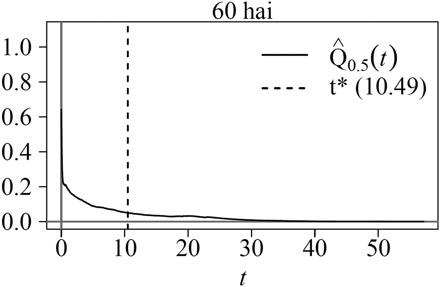
Estimated false discovery rate for the tomato microarray data set 60 hai. hai, hours after inoculation.

2.1. Methodology comparison

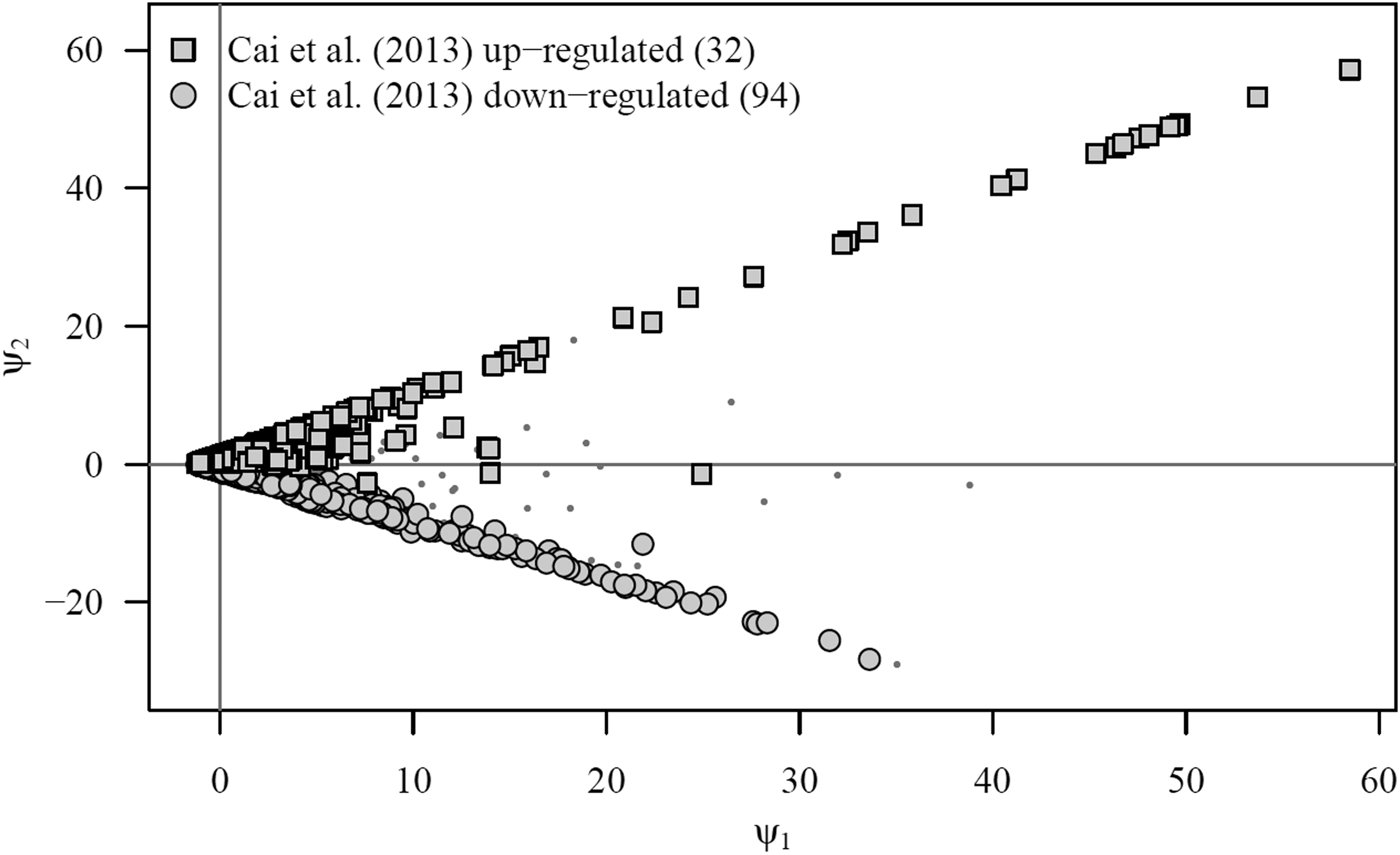
Cai et al. (2013) applied SAM and a two-factor (cultivar and time point) ANOVA to identify differentially expressed genes between IL6-2 tomato plants forming a part of the PI data set and, on the other, a different near isogenic tomato line (M82). Although the authors' principal objectives diverged from our own, results obtained on IL6-2 allow us to compare the results (Table 1; Figs. 2 and 3).

FIG. 2.

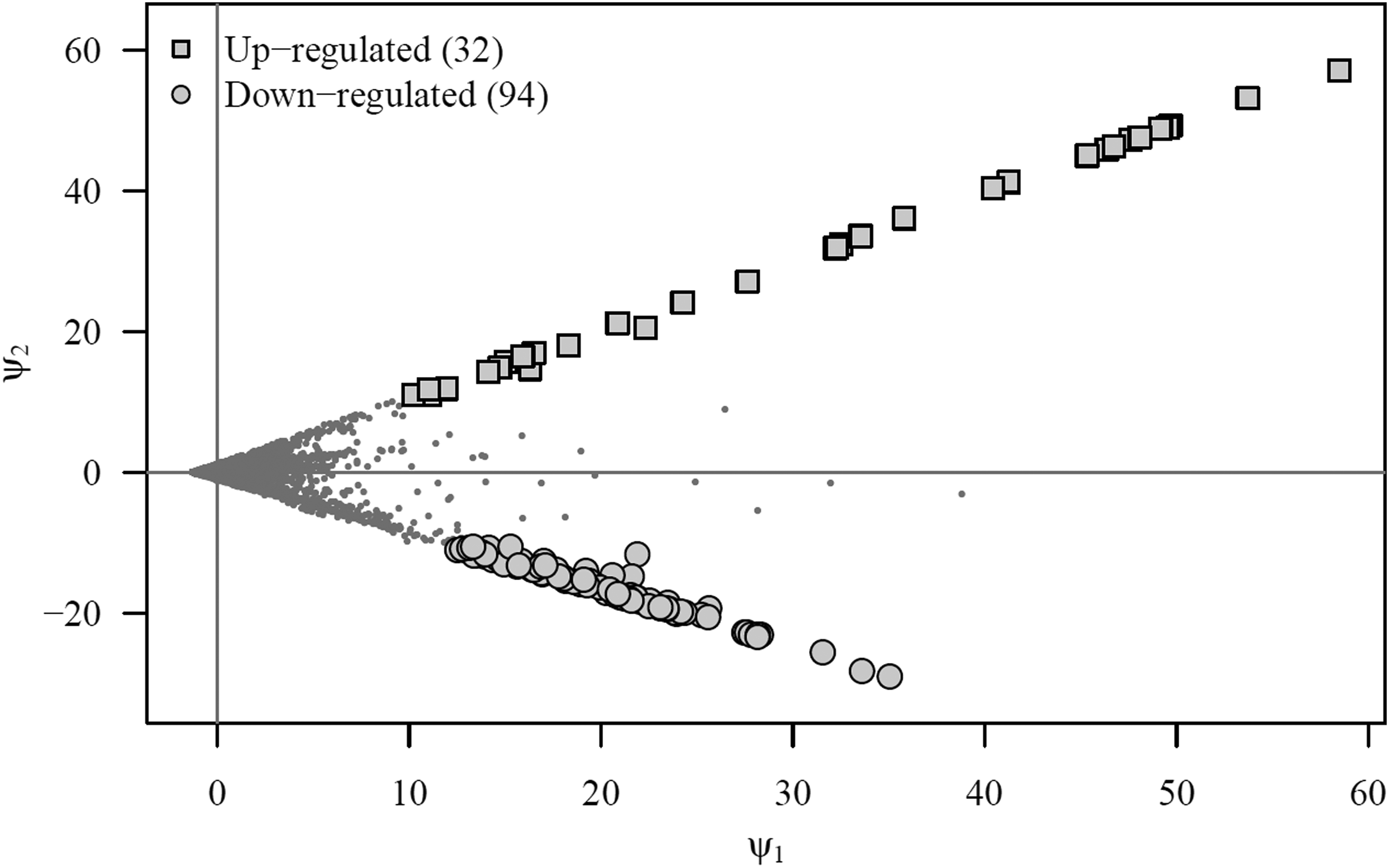
Projection of genes on the artificial components and differentially expressed genes in the PI microarray data set 60 hai detected by acde. See also Table 1.

FIG. 3.

Projection of genes on the artificial components and differentially expressed genes in the PI microarray data set 60 hai detected by Cai et al. (2013). See also Table 1.

Table 1.

Comparison of Differentially Expressed Genes Between acde and Previous Reported Results

acde	Cai et al. (2013)
acde	Upregulated	Downregulated	No differential expression	Total
Upregulated	30	0	2	32
Downregulated	0	41	53	94
No differential expression	803	1127	11,384	13,314
Total	833	1168	11,439	13,440

Genes are also highlighted on artificial components shown in Figures 2 and 3. See Cai et al. (2013).

While our method found 2 upregulated and 53 downregulated genes unidentified by Cai et al. (2013), they still identified a much larger number of differentially expressed genes. This is a consequence of row standardization as required by ANOVA and SAM and their corresponding univariate point of view. Indeed, when row standardization is performed, the inherent scale of genetic expression in the microarray is lost for further analysis.

To see this, note that a very large number of the genes identified by Cai et al. (2013) lie very close to the origin of the artificial plane in Figure 3, which means that their overall expression levels are very close to the average overall expression level in the microarray experiment. If Biological Scenario 2 holds, this is an important error because genes with no expression (those near the origin) are being identified as differentially expressed. Thus, the value of a multivariate point of view and the reason why our method should be preferred when Biological Scenario 2 is more likely to hold.

The results obtained on the 26 data sets on neurodegenerative diseases show that, in a general way, lower FDRs were obtained with acde, and they were much easier to tune when active differentially expressed genes are searched (Supplementary Algorithm 1).

3. Discussion

The present article outlines a multivariate approach for the identification of differentially expressed genes in gene expression data. Despite relying on a general probabilistic model, our methodology's applicability is rooted in the key biological and technical assumptions for gene expression data summarized in Biological Scenario 2. If such assumptions are correct, as is generally the case for microarray data, a multivariate approach is needed to obviate the (mis)identification of unexpressed genes as differentially expressed. Surprisingly, though, no multivariate inferential approach suitable for Biological Scenario 2 has been previously proposed.

Our methodology departs from Storey and Tibshirani's (2001) work on FDR estimation and the construction of two artificial components. These artificial components resemble the data's PCs, which generally reflect gene expression level in the first PC and differences between conditions in the second PC as already pointed out by the Kim et al. (2007) and their proposed parametric covariance matrix data transformation. Nevertheless, the here proposed artificial components offer an exact interpretation in terms of overall and differential genetic expression because they are constructed artificially directly computing mean expression differences. Storey and Tibshirani's (2001) research grants insight into both the validity of Biological Scenario 2 and the behavior of differential expression processes.

Here, we have suggested additional assessments that establish greater statistical confidence with respect to the results obtained via our methodology, such as BCa upper confidence bound for FDR. In sum, these complements represent the final pieces of an integral strategy aimed at identifying differentially expressed genes in microarray data.

At 60 hai, our analysis of the PI data set found 32 defense-related genes identified as upregulated and 94 primary metabolic function-related genes identified as downregulated. Comparing the above-mentioned findings with previous results (Cai et al., 2013), we observe that traditional methods place large number of differentially expressed genes close to the origin of the artificial plane. This led us to deduce two important problems in methods based on univariate statistics: data regarding overall gene activity in the inherent genetic expression scale were lost and genes with true zero expression levels were possibly wrongly categorized as differentially expressed.

On balance, it is safe to say that univariate-oriented methods identify more genes as differentially expressed, but FDRs are generally higher, a problem associated with differences in the biological assumptions underpinning this type of method and corresponding implied definitions of differential expression. Therefore, an examination of the numbers does not paint any method as more powerful in terms of a multiple testing procedure. That being said, when a study looks to perform an intervention on differentially expressed genes, our methodology demonstrates greater value insofar as it prevents intervention on unexpressed genes. The detection of active differentially expressed genes is also important when the procedure is used as a filter for the construction of a network. Genes with very low expression are not desired on a network.

4. Methods

4.1. Artificial components

Let Z represent a \documentclass{aastex}\usepackage{amsbsy}\usepackage{amsfonts}\usepackage{amssymb}\usepackage{bm}\usepackage{mathrsfs}\usepackage{pifont}\usepackage{stmaryrd}\usepackage{textcomp}\usepackage{portland, xspace}\usepackage{amsmath, amsxtra}\usepackage{upgreek}\pagestyle{empty}\DeclareMathSizes{10}{9}{7}{6}\begin{document} $$n \times p$$ \end{document} matrix where the rows correspond to the genes and the columns to the replicates in a microarray experiment. Also, let C be the columns and G be the rows of Z , genes in G being treated as the individuals of the analysis. We first standardize Z with respect to its column's means and variances for obtaining a new matrix X suitable for a PCA as follows: \documentclass{aastex}\usepackage{amsbsy}\usepackage{amsfonts}\usepackage{amssymb}\usepackage{bm}\usepackage{mathrsfs}\usepackage{pifont}\usepackage{stmaryrd}\usepackage{textcomp}\usepackage{portland, xspace}\usepackage{amsmath, amsxtra}\usepackage{upgreek}\pagestyle{empty}\DeclareMathSizes{10}{9}{7}{6}\begin{document} \begin{align*} { x_ { ij } } = { \frac { { z_ { ij } } - { { \overline { \bf z } } _j } } { s.e. \left( { { { \bf z } _j } } \right) } } , \;i \in G , \;j \; \in C , \tag { 1 } \end{align*} \end{document}

where z_j is the j-th column of Z .

Usually, in a PCA of microarray data, the first PC will mainly explain gene expression and the second one will mainly explain differential expression between conditions. However, to perform multiple tests regarding genetic differential expression, we need new components that exactly capture the genes' overall and differential expression levels. We call these components artificial because they do not arise naturally from solving a maximization problem (as do the PCs in a PCA). Instead, they are constructed deliberately to capture specific features of the data and thus have an exact interpretation. When Biological Scenario holds, they almost overlap with the first two PCs of a PCA because the first component tends to explain variability due to differences in gene expression between genes (mean) and the second one explains differences between conditions (mean differences). Their construction is as follows: For \documentclass{aastex}\usepackage{amsbsy}\usepackage{amsfonts}\usepackage{amssymb}\usepackage{bm}\usepackage{mathrsfs}\usepackage{pifont}\usepackage{stmaryrd}\usepackage{textcomp}\usepackage{portland, xspace}\usepackage{amsmath, amsxtra}\usepackage{upgreek}\pagestyle{empty}\DeclareMathSizes{10}{9}{7}{6}\begin{document} $$i \; = \;1 , \ldots , n$$ \end{document} , let the overall, the treatment, and the control means for gene i be: \documentclass{aastex}\usepackage{amsbsy}\usepackage{amsfonts}\usepackage{amssymb}\usepackage{bm}\usepackage{mathrsfs}\usepackage{pifont}\usepackage{stmaryrd}\usepackage{textcomp}\usepackage{portland, xspace}\usepackage{amsmath, amsxtra}\usepackage{upgreek}\pagestyle{empty}\DeclareMathSizes{10}{9}{7}{6}\begin{document} \begin{align*} { \overline x _ { i. } } = \frac { 1 } { p } \mathop \sum \limits_ { j = 1 } ^p { x_ { ij } } ; \ \ \ \ { \overline x _ { iTr } } = \frac { 1 } { { { p_1 } } } \mathop \sum \limits_ { j = 1 } ^ { { p_1 } } { x_ { ij } } ; \quad \quad { \overline x _ { iC } } = \frac { 1 } { { { p_2 } } } \mathop \sum \limits_ { j = { p_1 } + 1 } ^p { x_ { ij } } . \tag { 2 } \end{align*} \end{document}

For p₁ treatment and p₂ control replicates with \documentclass{aastex}\usepackage{amsbsy}\usepackage{amsfonts}\usepackage{amssymb}\usepackage{bm}\usepackage{mathrsfs}\usepackage{pifont}\usepackage{stmaryrd}\usepackage{textcomp}\usepackage{portland, xspace}\usepackage{amsmath, amsxtra}\usepackage{upgreek}\pagestyle{empty}\DeclareMathSizes{10}{9}{7}{6}\begin{document} $$p \; = \;{p_1} \; + \;{p_2}$$ \end{document} . Define: \documentclass{aastex}\usepackage{amsbsy}\usepackage{amsfonts}\usepackage{amssymb}\usepackage{bm}\usepackage{mathrsfs}\usepackage{pifont}\usepackage{stmaryrd}\usepackage{textcomp}\usepackage{portland, xspace}\usepackage{amsmath, amsxtra}\usepackage{upgreek}\pagestyle{empty}\DeclareMathSizes{10}{9}{7}{6}\begin{document} \begin{align*} { \psi _1 } \left( { { x_ { i. } } } \right) = { \psi _ { 1i } } = \sqrt p \; { \overline x _ { i. } } ; \ \ \ { \psi _2 } \left( { { x_ { i. } } } \right) = { \psi _ { 2i } } = \; { \frac { \sqrt { { p_1 } { p_2 } } } { \sqrt { { p_1 } + { p_2 } } } } \left( { { { \overline x } _ { iTr } } - { { \overline x } _ { iC } } } \right). \tag { 3 } \end{align*} \end{document}

Now, \documentclass{aastex}\usepackage{amsbsy}\usepackage{amsfonts}\usepackage{amssymb}\usepackage{bm}\usepackage{mathrsfs}\usepackage{pifont}\usepackage{stmaryrd}\usepackage{textcomp}\usepackage{portland, xspace}\usepackage{amsmath, amsxtra}\usepackage{upgreek}\pagestyle{empty}\DeclareMathSizes{10}{9}{7}{6}\begin{document} $${ \psi _{1i}}$$ \end{document} is just a multiple of the mean expression level of gene i across both conditions, so it captures its overall expression level. As the data have not been standardized by rows, \documentclass{aastex}\usepackage{amsbsy}\usepackage{amsfonts}\usepackage{amssymb}\usepackage{bm}\usepackage{mathrsfs}\usepackage{pifont}\usepackage{stmaryrd}\usepackage{textcomp}\usepackage{portland, xspace}\usepackage{amsmath, amsxtra}\usepackage{upgreek}\pagestyle{empty}\DeclareMathSizes{10}{9}{7}{6}\begin{document} $${ \psi_{1i}} > { \psi_{1i}} \prime$$ \end{document} implies that gene i has a higher overall expression level than gene \documentclass{aastex}\usepackage{amsbsy}\usepackage{amsfonts}\usepackage{amssymb}\usepackage{bm}\usepackage{mathrsfs}\usepackage{pifont}\usepackage{stmaryrd}\usepackage{textcomp}\usepackage{portland, xspace}\usepackage{amsmath, amsxtra}\usepackage{upgreek}\pagestyle{empty}\DeclareMathSizes{10}{9}{7}{6}\begin{document} $$i \prime$$ \end{document} , and thus, \documentclass{aastex}\usepackage{amsbsy}\usepackage{amsfonts}\usepackage{amssymb}\usepackage{bm}\usepackage{mathrsfs}\usepackage{pifont}\usepackage{stmaryrd}\usepackage{textcomp}\usepackage{portland, xspace}\usepackage{amsmath, amsxtra}\usepackage{upgreek}\pagestyle{empty}\DeclareMathSizes{10}{9}{7}{6}\begin{document} $${ \psi _1} = \left( {{ \psi _{11}} , \; \ldots , { \psi _{1n}}} \right)$$ \end{document} provides a natural scale for comparing expression levels between the genes in the microarray. Moreover, this natural scale, pooled from all the genes in the microarray, permits to identify genes that have no expression whatsoever under Biological Scenario 2. In PCA vocabulary (Lebart et al., 1995), \documentclass{aastex}\usepackage{amsbsy}\usepackage{amsfonts}\usepackage{amssymb}\usepackage{bm}\usepackage{mathrsfs}\usepackage{pifont}\usepackage{stmaryrd}\usepackage{textcomp}\usepackage{portland, xspace}\usepackage{amsmath, amsxtra}\usepackage{upgreek}\pagestyle{empty}\DeclareMathSizes{10}{9}{7}{6}\begin{document} $${ \psi _1}$$ \end{document} is a size component.

However, \documentclass{aastex}\usepackage{amsbsy}\usepackage{amsfonts}\usepackage{amssymb}\usepackage{bm}\usepackage{mathrsfs}\usepackage{pifont}\usepackage{stmaryrd}\usepackage{textcomp}\usepackage{portland, xspace}\usepackage{amsmath, amsxtra}\usepackage{upgreek}\pagestyle{empty}\DeclareMathSizes{10}{9}{7}{6}\begin{document} $${ \psi _{2i}}$$ \end{document} is a multiple of the difference between treatment and control mean expression levels, so it captures the amount to which gene i is differentially expressed. We call \documentclass{aastex}\usepackage{amsbsy}\usepackage{amsfonts}\usepackage{amssymb}\usepackage{bm}\usepackage{mathrsfs}\usepackage{pifont}\usepackage{stmaryrd}\usepackage{textcomp}\usepackage{portland, xspace}\usepackage{amsmath, amsxtra}\usepackage{upgreek}\pagestyle{empty}\DeclareMathSizes{10}{9}{7}{6}\begin{document} $${ \psi _2} = \left( {{ \psi _{21}} , \; \ldots , \;{ \psi _{2n}}} \right)$$ \end{document} a differential expression component. Large positive (negative) values of \documentclass{aastex}\usepackage{amsbsy}\usepackage{amsfonts}\usepackage{amssymb}\usepackage{bm}\usepackage{mathrsfs}\usepackage{pifont}\usepackage{stmaryrd}\usepackage{textcomp}\usepackage{portland, xspace}\usepackage{amsmath, amsxtra}\usepackage{upgreek}\pagestyle{empty}\DeclareMathSizes{10}{9}{7}{6}\begin{document} $${ \psi _{2i}}$$ \end{document} indicate high (low) expression levels in the treatment replicates and low (high) expression levels in the control replicates. The multiplicative constants in Equation (3) are defined so that \documentclass{aastex}\usepackage{amsbsy}\usepackage{amsfonts}\usepackage{amssymb}\usepackage{bm}\usepackage{mathrsfs}\usepackage{pifont}\usepackage{stmaryrd}\usepackage{textcomp}\usepackage{portland, xspace}\usepackage{amsmath, amsxtra}\usepackage{upgreek}\pagestyle{empty}\DeclareMathSizes{10}{9}{7}{6}\begin{document} $${ \psi _1}$$ \end{document} and \documentclass{aastex}\usepackage{amsbsy}\usepackage{amsfonts}\usepackage{amssymb}\usepackage{bm}\usepackage{mathrsfs}\usepackage{pifont}\usepackage{stmaryrd}\usepackage{textcomp}\usepackage{portland, xspace}\usepackage{amsmath, amsxtra}\usepackage{upgreek}\pagestyle{empty}\DeclareMathSizes{10}{9}{7}{6}\begin{document} $${ \psi _2}$$ \end{document} are the result of an orthogonal projection via unit projection vectors as in the PCA framework.

Under Biological Scenario 2, a gene can have large positive or large negative values of \documentclass{aastex}\usepackage{amsbsy}\usepackage{amsfonts}\usepackage{amssymb}\usepackage{bm}\usepackage{mathrsfs}\usepackage{pifont}\usepackage{stmaryrd}\usepackage{textcomp}\usepackage{portland, xspace}\usepackage{amsmath, amsxtra}\usepackage{upgreek}\pagestyle{empty}\DeclareMathSizes{10}{9}{7}{6}\begin{document} $${ \psi _{2i}}$$ \end{document} , if and only if it also has large positive values of \documentclass{aastex}\usepackage{amsbsy}\usepackage{amsfonts}\usepackage{amssymb}\usepackage{bm}\usepackage{mathrsfs}\usepackage{pifont}\usepackage{stmaryrd}\usepackage{textcomp}\usepackage{portland, xspace}\usepackage{amsmath, amsxtra}\usepackage{upgreek}\pagestyle{empty}\DeclareMathSizes{10}{9}{7}{6}\begin{document} $${ \psi _{1i}}$$ \end{document} . As a result, when \documentclass{aastex}\usepackage{amsbsy}\usepackage{amsfonts}\usepackage{amssymb}\usepackage{bm}\usepackage{mathrsfs}\usepackage{pifont}\usepackage{stmaryrd}\usepackage{textcomp}\usepackage{portland, xspace}\usepackage{amsmath, amsxtra}\usepackage{upgreek}\pagestyle{empty}\DeclareMathSizes{10}{9}{7}{6}\begin{document} $${ \psi _2}$$ \end{document} is used to identify differentially expressed genes, nonexpressed genes are automatically discarded by means of the natural scale ( \documentclass{aastex}\usepackage{amsbsy}\usepackage{amsfonts}\usepackage{amssymb}\usepackage{bm}\usepackage{mathrsfs}\usepackage{pifont}\usepackage{stmaryrd}\usepackage{textcomp}\usepackage{portland, xspace}\usepackage{amsmath, amsxtra}\usepackage{upgreek}\pagestyle{empty}\DeclareMathSizes{10}{9}{7}{6}\begin{document} $${ \psi _1}$$ \end{document} ) derived from a multivariate analysis of all the genes' expression levels in the microarray.

4.2. A word on scale

As a rule, methods that control the FDR in microarray data (Benjamini and Yuketeli, 2001; Storey and Tibshirani 2001; Tusher et al., 2001) use test statistics of the form \documentclass{aastex}\usepackage{amsbsy}\usepackage{amsfonts}\usepackage{amssymb}\usepackage{bm}\usepackage{mathrsfs}\usepackage{pifont}\usepackage{stmaryrd}\usepackage{textcomp}\usepackage{portland, xspace}\usepackage{amsmath, amsxtra}\usepackage{upgreek}\pagestyle{empty}\DeclareMathSizes{10}{9}{7}{6}\begin{document} \begin{align*} s ( { x_ { i. } } ) = { \frac { { { \overline x } _ { iTr } } - { { \overline x } _ { iC } } } { s.e. \left( { { { \overline x } _ { iTr } } - { { \overline x } _ { iC } } } \right) + { c_O } } } , \tag { 4 } \end{align*} \end{document}

where c₀ is a convenient constant (usually 0) or monotone functions of s as p values. However, when dividing by the standard error in Equation (4), we lose the inherent genetic expression scale that lies within the data, and genes with very low expression levels will be detected as differentially expressed. Nevertheless, the most common scenario is that only a very small fraction of the genes have high activities (Biological Scenario 2) as defined below.

Biological Scenario 1: All genes among all replicates have true positive expression levels when the sample is taken. Therefore, the major differences in scale between the genes are due to external sources of variation.

Biological Scenario 2: Only a small proportion of the genes in each replicate have true positive expression levels when the sample is taken and no systematic sources of variation other than the control/treatment effect are present in the experiment. Therefore, the major differences in scale between the genes are due to whether a gene was actively transcribing when the sample was taken. Here, the majority of genes should lie close to the origin of the artificial plane ( \documentclass{aastex}\usepackage{amsbsy}\usepackage{amsfonts}\usepackage{amssymb}\usepackage{bm}\usepackage{mathrsfs}\usepackage{pifont}\usepackage{stmaryrd}\usepackage{textcomp}\usepackage{portland, xspace}\usepackage{amsmath, amsxtra}\usepackage{upgreek}\pagestyle{empty}\DeclareMathSizes{10}{9}{7}{6}\begin{document} $${ \psi _1}$$ \end{document} vs. \documentclass{aastex}\usepackage{amsbsy}\usepackage{amsfonts}\usepackage{amssymb}\usepackage{bm}\usepackage{mathrsfs}\usepackage{pifont}\usepackage{stmaryrd}\usepackage{textcomp}\usepackage{portland, xspace}\usepackage{amsmath, amsxtra}\usepackage{upgreek}\pagestyle{empty}\DeclareMathSizes{10}{9}{7}{6}\begin{document} $${ \psi _2}$$ \end{document} ), and only a few (the active genes) should lie far to the right.

If Scenario 1 holds, there is no relevant information in the differences between the scales of the rows in the data, and row standardization is in order. If, on the contrary, Scenario 2 seems more appropriate, the information contained in the differences between the scales of the rows is relevant for it allows to asses which genes had actual positive expression levels when the sample was taken.

Likewise, if Scenario 2 holds, the data for the genes that were not expressing themselves when the sample was taken are only the results of external sources of variation. Those genes, having true zero expression levels in both treatment and control replicates, cannot be classified as being differentially expressed. However, because n is very large and there might be systematic sources of variation (changes in printing tips, background intensity, or other aspects of microarray technology), it is very likely that a considerable number of those genes with no expression will be identified as differentially expressed when using statistics of the form in Equation (4).

We strongly believe that the first condition of Biological Scenario 2 is more reasonable in the context of microarray experiments. Additionally, there are several methods for normalization of gene expression data that remove systematic sources of variation other than control/treatment effects, without performing any kind of row standardization (Dudoit et al., 2002; Simon et al., 2003). These methods can be applied beforehand to assure the technical part of Biological Scenario 2. To conclude, row standardization should not be performed, to avoid identifying genes with no expression as differentially expressed, because this standardization eliminates natural gene differences making all gene expression levels very similar. If a scenario in between seems more likely, Scenario 2 should be favored.

4.3. Detection of differentially expressed genes with acde

4.3.1. Estimation

Our methodology aims at identifying differentially expressed genes in gene expression data while controlling the FDR at a desired level (Storey and Tibshirani, 2001; Storey et al., 2004). For controlling the FDR, researchers can turn to one of the two distinct approaches to multiple hypothesis testing: while one establishes a desired FDR level and estimates a rejection region, the other proceeds in reverse order (establishes a rejection region before estimating the FDR). Storey et al. (2004) showed that these two approaches are asymptotically equivalent. More specifically, they define: . Then, rejecting all null hypothesis with 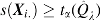proves tantamount to establishing FDR control at level \documentclass{aastex}\usepackage{amsbsy}\usepackage{amsfonts}\usepackage{amssymb}\usepackage{bm}\usepackage{mathrsfs}\usepackage{pifont}\usepackage{stmaryrd}\usepackage{textcomp}\usepackage{portland, xspace}\usepackage{amsmath, amsxtra}\usepackage{upgreek}\pagestyle{empty}\DeclareMathSizes{10}{9}{7}{6}\begin{document} $$\alpha$$ \end{document} , for n large enough. In other words, Algorithm 1 controls the FDR at level \documentclass{aastex}\usepackage{amsbsy}\usepackage{amsfonts}\usepackage{amssymb}\usepackage{bm}\usepackage{mathrsfs}\usepackage{pifont}\usepackage{stmaryrd}\usepackage{textcomp}\usepackage{portland, xspace}\usepackage{amsmath, amsxtra}\usepackage{upgreek}\pagestyle{empty}\DeclareMathSizes{10}{9}{7}{6}\begin{document} $$\alpha$$ \end{document} .

The following observations regarding Algorithm 1 may be made: 1.

is considered conservatively biases, that is, (Storey and Tibshirani, 2001).

FDR is only estimated for t at the values at which the number of rejected hypotheses is actually affected. More specifically, let \documentclass{aastex}\usepackage{amsbsy}\usepackage{amsfonts}\usepackage{amssymb}\usepackage{bm}\usepackage{mathrsfs}\usepackage{pifont}\usepackage{stmaryrd}\usepackage{textcomp}\usepackage{portland, xspace}\usepackage{amsmath, amsxtra}\usepackage{upgreek}\pagestyle{empty}\DeclareMathSizes{10}{9}{7}{6}\begin{document} $${t_{ \left[ 1 \right] }} \ldots {t_{ \left[ n \right] }}$$ \end{document} be the ordered values of \documentclass{aastex}\usepackage{amsbsy}\usepackage{amsfonts}\usepackage{amssymb}\usepackage{bm}\usepackage{mathrsfs}\usepackage{pifont}\usepackage{stmaryrd}\usepackage{textcomp}\usepackage{portland, xspace}\usepackage{amsmath, amsxtra}\usepackage{upgreek}\pagestyle{empty}\DeclareMathSizes{10}{9}{7}{6}\begin{document} $$\tau = \left\{ { \left\vert {{ \psi _{2i}}} \right\vert: i = 1 , \ldots , n} \right\} $$ \end{document} . Then, using \documentclass{aastex}\usepackage{amsbsy}\usepackage{amsfonts}\usepackage{amssymb}\usepackage{bm}\usepackage{mathrsfs}\usepackage{pifont}\usepackage{stmaryrd}\usepackage{textcomp}\usepackage{portland, xspace}\usepackage{amsmath, amsxtra}\usepackage{upgreek}\pagestyle{empty}\DeclareMathSizes{10}{9}{7}{6}\begin{document} $$\left[ {t \left[ k \right] , \infty } \right)$$ \end{document} as the rejection region produces k genes identified as differentially expressed.

To streamline computation, we set \documentclass{aastex}\usepackage{amsbsy}\usepackage{amsfonts}\usepackage{amssymb}\usepackage{bm}\usepackage{mathrsfs}\usepackage{pifont}\usepackage{stmaryrd}\usepackage{textcomp}\usepackage{portland, xspace}\usepackage{amsmath, amsxtra}\usepackage{upgreek}\pagestyle{empty}\DeclareMathSizes{10}{9}{7}{6}\begin{document} $$\lambda = 0.5$$ \end{document} , following Storey et al. (2004) and Storey and Tibshirani (2001). However, a more suitable \documentclass{aastex}\usepackage{amsbsy}\usepackage{amsfonts}\usepackage{amssymb}\usepackage{bm}\usepackage{mathrsfs}\usepackage{pifont}\usepackage{stmaryrd}\usepackage{textcomp}\usepackage{portland, xspace}\usepackage{amsmath, amsxtra}\usepackage{upgreek}\pagestyle{empty}\DeclareMathSizes{10}{9}{7}{6}\begin{document} $$\lambda$$ \end{document} in terms of the mean square error of can be computed via bootstrap methods.

The estimation of in step 2 may be carried out by using permutation or bootstrap estimates of the statistics' null distribution (Dudoit and Van Der Laan, 2007). Although permutation methods are more frequently used in the reference literature (Li and Tibshirani, 2013), we have opted for bootstrap estimates of the null distribution because they over greater ease of interpretation (Dudoit et al., 2008, p. 65). Whether permutation or bootstraps are used, results should prove very similar for large B (Efron and Tibshirani, 1993).

\documentclass{aastex}\usepackage{amsbsy}\usepackage{amsfonts}\usepackage{amssymb}\usepackage{bm}\usepackage{mathrsfs}\usepackage{pifont}\usepackage{stmaryrd}\usepackage{textcomp}\usepackage{portland, xspace}\usepackage{amsmath, amsxtra}\usepackage{upgreek}\pagestyle{empty}\DeclareMathSizes{10}{9}{7}{6}\begin{document} $$B =$$ \end{document} 100 should be enough for obtaining accurate and stable estimates in step 2 (Efron and Tibshirani, 1993).

Computation of the genes' Q-values (Storey, 2002, 2003) may provide useful insights.

We applied Storey and Tibshirani's methodology as explained above, but using a new proposed multivariate statistic that is well suited for gene expression data. It is based on the large sample estimator for the FDR, , presented for multiple testing procedures, but it uses \documentclass{aastex}\usepackage{amsbsy}\usepackage{amsfonts}\usepackage{amssymb}\usepackage{bm}\usepackage{mathrsfs}\usepackage{pifont}\usepackage{stmaryrd}\usepackage{textcomp}\usepackage{portland, xspace}\usepackage{amsmath, amsxtra}\usepackage{upgreek}\pagestyle{empty}\DeclareMathSizes{10}{9}{7}{6}\begin{document} $$s ( {x_{i.}} ) = \left\vert {{ \psi _{2i}}} \right\vert$$ \end{document} as the test statistic. Our method is presented in Algorithm 1.

Algorithm 1: Identification of differentially expressed genes in gene expression data for a single time point.
1. Compute \documentclass{aastex}\usepackage{amsbsy}\usepackage{amsfonts}\usepackage{amssymb}\usepackage{bm}\usepackage{mathrsfs}\usepackage{pifont}\usepackage{stmaryrd}\usepackage{textcomp}\usepackage{portland, xspace}\usepackage{amsmath, amsxtra}\usepackage{upgreek}\pagestyle{empty}\DeclareMathSizes{10}{9}{7}{6}\begin{document} $$\left\vert {{ \psi _{2i}}} \right\vert = { \psi _2} \left( {{x_{i.}}} \right)$$ \end{document} . For \documentclass{aastex}\usepackage{amsbsy}\usepackage{amsfonts}\usepackage{amssymb}\usepackage{bm}\usepackage{mathrsfs}\usepackage{pifont}\usepackage{stmaryrd}\usepackage{textcomp}\usepackage{portland, xspace}\usepackage{amsmath, amsxtra}\usepackage{upgreek}\pagestyle{empty}\DeclareMathSizes{10}{9}{7}{6}\begin{document} $$i = 1 , \ldots , n \;$$ \end{document} from Equation (3).
2. For each t in \documentclass{aastex}\usepackage{amsbsy}\usepackage{amsfonts}\usepackage{amssymb}\usepackage{bm}\usepackage{mathrsfs}\usepackage{pifont}\usepackage{stmaryrd}\usepackage{textcomp}\usepackage{portland, xspace}\usepackage{amsmath, amsxtra}\usepackage{upgreek}\pagestyle{empty}\DeclareMathSizes{10}{9}{7}{6}\begin{document} $$\tau = \left\{ { \left\vert {{ \psi _{2i}}} \right\vert , \ldots , \left\vert {{ \psi _{2n}}} \right\vert } \right\} $$ \end{document} and B large enough, compute with \documentclass{aastex}\usepackage{amsbsy}\usepackage{amsfonts}\usepackage{amssymb}\usepackage{bm}\usepackage{mathrsfs}\usepackage{pifont}\usepackage{stmaryrd}\usepackage{textcomp}\usepackage{portland, xspace}\usepackage{amsmath, amsxtra}\usepackage{upgreek}\pagestyle{empty}\DeclareMathSizes{10}{9}{7}{6}\begin{document} $$\lambda = 0.5$$ \end{document} and test statistic \documentclass{aastex}\usepackage{amsbsy}\usepackage{amsfonts}\usepackage{amssymb}\usepackage{bm}\usepackage{mathrsfs}\usepackage{pifont}\usepackage{stmaryrd}\usepackage{textcomp}\usepackage{portland, xspace}\usepackage{amsmath, amsxtra}\usepackage{upgreek}\pagestyle{empty}\DeclareMathSizes{10}{9}{7}{6}\begin{document} $$\; \left\vert {{ \psi _{2i}}} \right\vert$$ \end{document} .
3. Set a desired FDR level at \documentclass{aastex}\usepackage{amsbsy}\usepackage{amsfonts}\usepackage{amssymb}\usepackage{bm}\usepackage{mathrsfs}\usepackage{pifont}\usepackage{stmaryrd}\usepackage{textcomp}\usepackage{portland, xspace}\usepackage{amsmath, amsxtra}\usepackage{upgreek}\pagestyle{empty}\DeclareMathSizes{10}{9}{7}{6}\begin{document} $${ \alpha ^<sup>*</sup>}$$ \end{document} and compute .
4. Identify a set of differentially expressed genes as \documentclass{aastex}\usepackage{amsbsy}\usepackage{amsfonts}\usepackage{amssymb}\usepackage{bm}\usepackage{mathrsfs}\usepackage{pifont}\usepackage{stmaryrd}\usepackage{textcomp}\usepackage{portland, xspace}\usepackage{amsmath, amsxtra}\usepackage{upgreek}\pagestyle{empty}\DeclareMathSizes{10}{9}{7}{6}\begin{document} $${ \mathcal{R}_{{t^<sup></sup>}}} = \left\{ {i: \left\vert {{ \psi _{2i}}} \right\vert \ge {t^<sup></sup>}} \right\} $$ \end{document} .

For more details, see Supplementary Algorithm 1.

4.3.2. Further assessments

As B, n, and p grow, approaches from above both the FDR and the realized proportion of false positives among all rejected null hypothesis. In practice, however, because B, n, and p are finite, the control achieved using is only approximate and some additional assessments are needed. Storey and Tibshirani (2001) suggested the use of a bootstrap percentile upper confidence bound for the FDR to provide a somewhat more precise notion of the actual control achieved but concluded that percentile upper bounds were not appropriate as they underestimated the actual confidence upper bound. We overcome this limitation by computing a BCa upper confidence bound (Efron and Tibshirani, 1993) for the FDR as shown in Algorithm 2. We find plots of and the FDRs confidence upper bounds versus t to be very informative as to the actual FDR control achieved.

Algorithm 2: Computation of a BCa upper confidence bound for the FDR.
1. Compute by applying steps 1 and 2 of Algorithm 1.
2. Compute a large number of R independent bootstrap samples.
3. Compute bootstrap replicates of by applying steps 1 and 2 of Algorithm 1 for t in \documentclass{aastex}\usepackage{amsbsy}\usepackage{amsfonts}\usepackage{amssymb}\usepackage{bm}\usepackage{mathrsfs}\usepackage{pifont}\usepackage{stmaryrd}\usepackage{textcomp}\usepackage{portland, xspace}\usepackage{amsmath, amsxtra}\usepackage{upgreek}\pagestyle{empty}\DeclareMathSizes{10}{9}{7}{6}\begin{document} $$\tau$$ \end{document} .
4. For each t in \documentclass{aastex}\usepackage{amsbsy}\usepackage{amsfonts}\usepackage{amssymb}\usepackage{bm}\usepackage{mathrsfs}\usepackage{pifont}\usepackage{stmaryrd}\usepackage{textcomp}\usepackage{portland, xspace}\usepackage{amsmath, amsxtra}\usepackage{upgreek}\pagestyle{empty}\DeclareMathSizes{10}{9}{7}{6}\begin{document} $$\tau$$ \end{document} and the desired confidence level, compute the BCa confidence upper bound for .

For more details, see Supplementary Algorithm 2.

To illustrate our method, we will analyze the data set from the Tomato Expression Database web site (http://ted.bti.cornell.edu/), experiment E022 (Restrepo et al., 2005; PI data set). Throughout the experiment, eight tomato plants (line IL6-2) in field conditions were inoculated with Phytophthora infestans and eight control plants were mock-inoculated with sterile water. Leaf tissue samples from each replicate were taken at 12 hours before and 12, 36, and 60 hai. We refer to 12 hours before inoculation as the 0 hai time point. RNA was extracted from each sample and then hybridized on a complementary DNA microarray (for more details of the experimental design and conditions of the study, see Cai et al., 2013). Expression levels were obtained for 13,440 genes.

To further validate the method, 26 data sets on neurodegenerative disease are composed of 4 data sets of amyotrophic lateral sclerosis, 3 Alzheimer's disease data sets, 7 Parkinson's disease data sets, 8 multiple sclerosis data sets, and four schizophrenia data sets. For details on accession numbers, see Supplementary File.

Availability

The here presented method is available as a Bioconductor package (acde): https://www.bioconductor.org/packages/3.3/bioc/html/acde.html, https://www.bioconductor.org/packages/devel/bioc/html/acde.html

Footnotes

Acknowledgments

This research has been partially financed by a Grant of the Colombian Banco de la República (Project No. 3202) and the Universidad de Colombia—Sede Bogotá.

Author Disclosure Statement

The authors declare there are no competing financial interests.

Supplementary Material

References

Alizadeh

A.A.

, Eisen

M.B.

, Davis

R.E.

, et al. 2000. Distinct types of diffuse large b-cell lymphoma identified by gene expression profiling. Nature. 403, 503–511.

Benjamini

, and Hochberg

1995. Controlling the false discovery rate: A practical and powerful approach to multiple testing. J. R. Stat. Soc. Series B Methodol. 57, 289–300.

Benjamini

, and Yekutieli

2001. The control of the false discovery rate in multiple testing under dependency. Ann. Stat. 29, 1165–1188.

Cai

, Restrepo

, Myers

, et al. 2013. Gene profiling in partially resistant and susceptible near-isogenic tomatoes in response to late blight in the field. Mol. Plant. Pathol. 14, 171–184.

Dudoit

, and Van Der Laan

M.J

. 2007. Multiple Testing Procedures with Applications to Genomics. Springer, New York.

Dudoit

, Yang

Y.H.

, Callow

M.J.

, et al. 2002. Statistical methods for identifying differentially expressed genes in replicated cDNA microarray experiments. Statistica. Sinica. 12, 111–139.

Efron

, and Tibshirani

R.J.

1993. An Introduction to the Bootstrap. Chapman & Hall/CRC, New York.

Kerr

M.K.

, Martin

, and Churchill

G.A.

2000. Analysis of variance for gene expression microarray data. J. Comput. Biol. 7, 819–837.

Kim

, Zhang

, Jiang

, et al. 2007. Measuring similarities between gene expression profiles through new data transformations. BMC Bioinformatics. 8, 1–14.

10.

Lebart

, Morineau

, and Piron

1995. Statistique Exploratoire Multidimensionnelle. Dunod, Paris.

11.

, and Tibshiranin

2013. Finding consistent patterns: A nonparametric approach for identifying differential expression in RNA-Seq data. Stat. Methods Med. Res. 22, 519–536.

12.

Ospina

, and López-Kleine

2013. Identification of differentially expressed genes in microarray data in a principal component space. SpringerPlus. 2, 60.

13.

Restrepo

, Cai

, Fry

, et al. 2005. Gene expression profiling of infection of tomato by Phytophthora infestans in the fieeld. Phytopathology. 95, S88.

14.

Ross

D.T.

, Scherf

, Eisen

M.B.

, et al. 2000. Systematic variation in gene expression patterns in human cancer cell lines. Nat. Genet. 24, 227–235.

15.

Simon

R.M.

, Korn

E.L.

, McShane

L.M.

, et al. 2003. Design and Analysis of DNA Microarray Investigations. Springer, New York.

16.

Storey

J.D.

2002. A direct approach to false discovery rates. J. R. Stat. Soc. Series B Methodol. 64, 479–498.

17.

Storey

J.D.

2003. The positive false discovery rate: A Bayesian Interpretation and the q-value. Ann. Stat. 31, 2013–2035.

18.

Storey

J.D.

, Taylor

J.E.

, and Siegmund

2004. Strong control, conservative point estimation and simultaneous conservative consistency of false discovery rates: A unified approach. J. R. Stat. Soc. Series B Stat. Methodol. 66, 187–205.

19.

Storey

J.D.

, and Tibshirani

2001. Estimating false discovery rates under dependence, with applications to DNA microarrays. Technical Report. Department of Statistics, Stanford University.

20.

Taylor

, Tibshirani

, and Efron

2005. The “miss rate” for the analysis of gene expression data. Biostatistics. 6, 111–117.

21.

Tusher

V.G.

, Tibshirani

, and Chu

2001. Significance analysis of microarrays applied to the ionizing radiation response. Proc. Natl. Acad. Sci. U. S. A. 98, 5116–5121.

22.

Vélez

J.I.

, Correa

J.C.

, and Arcos-Burgos

2014. A new method for detecting significant p-values with applications to genetic data. Rev. Colomb. Estad. 37, 69–78.

23.

Xiong

, Brown

, Boley

, et al. 2014. DE-FPCA: Testing Gene Differential Expression and Exon Usage Through Functional Principal Component Analysis in Statistical Analysis of Next Generation Sequencing Data. Springer, New York, 129–143.

24.

Yuan

, and Kendziorski

2006. Hidden Markov models for microarray time course data in multiple biological conditions. J. Am. Stat. Assoc. 101, 1323–1332.

Supplementary Material

Please find the following supplemental material available below.

For Open Access articles published under a Creative Commons License, all supplemental material carries the same license as the article it is associated with.

For non-Open Access articles published, all supplemental material carries a non-exclusive license, and permission requests for re-use of supplemental material or any part of supplemental material shall be sent directly to the copyright owner as specified in the copyright notice associated with the article.

0.00 MB

0.78 MB