Integrated analysis of structural variants (SVs) and copy number alterations in aneuploid cancer genomes is key to understanding tumor genome complexity. A recently developed algorithm, Weaver, can estimate, for the first time, allele-specific copy number of SVs and their interconnectivity in aneuploid cancer genomes. However, one major limitation is that not all SVs identified by Weaver are phased. In this article, we develop a general convex programming framework that predicts the interconnectivity of unphased SVs with possibly noisy allele-specific copy number estimations as input. We demonstrated through applications to both simulated data and HeLa whole-genome sequencing data that our method is robust to the noise in the input copy numbers and can predict SV phasings with high specificity. We found that our method can make consistent predictions with Weaver even if a large proportion of the input variants are unphased. We also applied our method to The Cancer Genome Atlas (TCGA) ovarian cancer whole-genome sequencing samples to phase SVs left unphased by Weaver. Our work provides an important new algorithmic framework for recovering more complete allele-specific cancer genome graphs.
1. Introduction
A significant proportion of cancer genomes are aneuploid and have undergone somatic copy number alterations (CNAs), and even whole-genome duplications (WGDs) (Beroukhim et al., 2010; Gordon et al., 2012; Zack et al., 2013). Structural variants (SVs) that involve complex somatic rearrangements can further modify aneuploid cancer genomes. It has been shown that aneuploid cancer genomes typically have a higher rate of CNAs and SVs that happen together (Zack et al., 2013), and the mechanisms are related (Carvalho and Lupski, 2016). Therefore, it is important to analyze CNAs and SVs in an integrated manner in aneuploid cancer genomes to obtain a more complete view of the tumor genome complexity, which would in turn help us understand the somatic evolutionary history of cancer genomes (Greenman et al., 2012). In the past few years, many computational tools have been developed to infer SVs and CNAs individually (Van Loo et al., 2010; Wang et al., 2011; Carter et al., 2012), but none gives us a completely integrated view of how CNAs and SVs interact nor provides an allele-specific context to SVs.
We previously developed a new algorithm, Weaver (Li et al., 2016), which can simultaneously analyze SVs and allele-specific copy numbers of genomic regions (ASCNG) in the context of aneuploid cancer genome. Specifically, Weaver is able to identify allele-specific copy numbers of SVs (ASCNS) as well as the interconnectivity between them (i.e., phasing). Weaver uses a Markov Random Field, where ASCNS and SV phasing configuration, together with ASCNG, are hidden states in the nodes in the graph, and the observations include sequencing coverage and read linkage between SVs. The results from Li et al. (2016) demonstrated that Weaver can be successfully applied to cancer cell lines (MCF-7 and HeLa) as well as The Cancer Genome Atlas (TCGA) patient samples to generate base-pair resolution ASCNS and ASCNG with high accuracy.
However, one major limitation of Weaver is that it is not guaranteed to output a phasing for all SVs. In some tumor samples that we have tested, as few as 60% of the detected SVs may be phased by using the paired-end reads from the whole-genome sequencing sample together with the known single nucleotide polymorphism (SNP) phasing information from the 1000 Genomes Project. It is therefore important to develop additional approaches as a step further to predict the interconnectivity of allele-specific SVs and phase them into a more complete haplotype structure. Our motivation in this work is that we may be able to utilize the copy number information gathered to further predict phasing for the remaining allele-specific breakpoints. Such an approach could serve two useful purposes: (1) the predicted phasing structure would provide a more complete context for interpreting cancer-specific functional genomic data [such as Adey et al. (2013)]; and (2) the predicted phasing structure may offer insights into incorporating data from other technologies [such as physical maps (Gupta et al., 2015), PacBio (Eid et al., 2009; Adey et al., 2013), or 10 × Genomics (Zheng et al., 2016)], if available, to further solve somatic genome architecture at the haplotype level in aneuploid cancer genomes.
The goal of this work is to develop a new algorithm to fully leverage the output from Weaver to further improve SV phasing. Given copy number predictions from some source, for example, from sources such as Adey et al. (2013) or from Weaver, and a large number of putative unphased SVs, we wish to use the new algorithm to further predict SV phasing accurately. Here, we develop a convex optimization framework that minimizes a flow-like objective function while phasing the set of unphased SVs. We implement an integer linear program (ILP) derived from this framework and test it on both simulations and real data to demonstrate that our method is not sensitive to false positives, and robust to copy number noise in the input. We aim to extend this method to account for long read data in the future, and support the Weaver framework in obtaining a more complete description of a cancer genome.
2. Background
As we previously mentioned, one major limitation of Weaver is that it does not always phase all SVs. For example, of the 36 TCGA ovarian cancer patient samples we analyzed using Weaver in this article, the average fraction of unphased SVs is a little over 30% and many as 53% of the detected SVs (where the total number varies from 17 to 527) may be unphased in these samples. This may be due to low read support for the SV or due to balanced copy numbers for the bordering region alleles. Currently, Weaver also does not predict the phasing of copy number neutral events, such as inversions. On the contrary, we know that Weaver can produce accurate estimation of ASCNG in aneuploid tumor genomes (Li et al., 2016). Our goal here is to improve on, or predict, the phasing of SVs, given the allele-specific copy numbers (ASCNs). Note that in this work we do not seek information from germ line SNPs to help phasing as we assume that we have already exhausted the information from SNPs and the read linkage provided by the paired-end reads from the sequencing data.
2.1. Problem setting
Our input is a set of genomic regions and SVs. A genomic region is specified by a pair of loci (i.e., coordinates) on a chromosome in the reference genome, called the extremities of that genomic region. We assume that the set of all genomic regions is disjoint, that is, there are no two regions such that one or both extremities of one region lie between the extremities of the other. An SV is specified by a set of genomic loci, called breakpoints. These breakpoints need not lie on the same chromosome. Since Weaver infers pairs of breakpoints as SVs, we use the terms “pair of breakpoints” and SVs interchangeably. In the input, each genomic locus is associated with at most one breakpoint: this is called the infinite sites assumption (Kimura, 1969; Ma et al., 2008). This assumption comes as a natural consequence of the hypothesis that the probability of a single genomic site being subjected to an SV breakpoint is usually low. Formally, breakpoints may be assumed to occur randomly across the genome, following an unobserved probability distribution. If the number of genomic loci is very large, this distribution may be approximated by a continuous density function. Under this assumption, a genomic locus will almost surely not be used as a breakpoint more than once, even if some regions are more likely to host breakpoints than others. However, this assumption may be invalid if the breakpoints are resolved at a very low resolution. Therefore, in the context of providing a general framework, the infinite sites assumption can be ignored as a condition that is probably too strong in real data.
The normal human genome is diploid, where each genomic region on a chromosome can be associated with two alleles. Specifically, it is possible to differentiate between chromosome regions that arise from the paternal copy of the chromosome, and those that come from the maternal copy of the chromosome. In a noncancerous genome, for most genomic regions, we expect exactly one copy of a chromosomal region from each allele. In a tumor genome, on the contrary, due to somatic CNAs and SVs, as well as aneuploidy, we frequently find multiple copies of allelic regions, or regions from a specific allele that are lost (loss of heterozygosity). It is now acknowledged that CNAs and WGDs are prevalent in various types of cancer genomes (Zack et al., 2013). Therefore, it is important to accurately characterize the allele-specific copy number of a genomic region in the tumor genome. Furthermore, SVs and CNAs in cancer genomes could lead to a rearranged haplotype structure and a different interconnectivity of the SVs from that seen in the noncancerous genome. Thus, if we can identify the connections among different SVs at the haplotype level (i.e., providing a phasing), we can specify the haplotype that the breakpoints lie in, resolving the complexity of aneuploid cancer genomes at a fine-grained level. We can also associate an ASCN to SVs, based on how many times the phased variant is found in the tumor genome. ASCNS is also estimated through Weaver (Li et al., 2016).
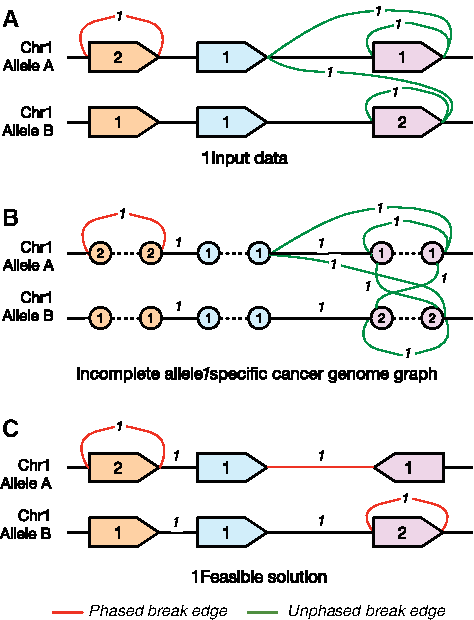
Figure 1A shows an example of how a cancer genome may compare to a normal genome. The figure shows two copies of the same chromosome, with blocks representing regions, black edges representing connections between regions that were adjacent in the normal genome, and colored edges representing connections between regions that are detected in the cancer genome. Red edges are adjacencies representing SVs that are phased. Green edges represent a possible phased configuration of an unphased SV. The numbers depict the number of copies of each region/SV. The goal is to predict a phasing of the SVs represented by the green edges, which translates to setting the ASCN of other possibilities to 0, that minimizes an objective function that corresponds to “discordant” ASCN information in the input data.
An example of an incomplete allele-specific cancer genome graph showing two alleles of the same chromosome. (A) Shows the problem setting, where two copies of the same chromosome are given. Genomic regions are given as blocks, adjacencies between blocks present in the reference genome are shown in black, and SVs are given by colored edges. Phased SVs, with the allele of both breakpoints known, are in red, and those that are unphased are in green. ASCNs for both genomic regions and SVs are shown as numbers near the regions/edges. If an SV is unphased, there are many possibilities for the correct phasing. (B) Shows the translation into an incomplete allele-specific cancer genome graph, with regions being replaced by 2 vertices each, and copy numbers assigned to all SVs and possible noncancer edges. This is the instance on which the objective (3) is defined. A correct solution will modify the copy numbers of the edges to minimize (3), selecting one of the many possible SVs. (C) Shows a feasible solution to the toy problem presented. Edges with assigned copy number 0 in this solution are not shown, and the SVs that are phased are now given in red. ASCN, allele-specific copy number; SV, structural variant.
2.2. Method overview
Using the regions and SVs, and their corresponding ASCNs as predicted by Weaver as input, we can construct an allele-specific cancer genome graph. In such a graph, we represent different alleles of a region by different vertices. Specifically, we represent each region extremity by two vertices, each representing a different allele with the corresponding ASCN. Two vertices are adjacent to each other if the corresponding allele-specific regions occurred next to each other in the tumor genome, that is, they either represent a putative SV with allele-specific breakpoints, or the adjacency has never been broken in the cancer genome. In the resulting graph, there may be breakpoints adjacent to more than one SV edge, representing the possible phasings of an SV. Thus, the graph is incomplete, in the sense that there is a set of edges in the graph that are not representative of the actual adjacency information in the tumor sample. If all the SVs were phased, and all ASCNs were predicted correctly, the copy number of an allele-specific region should be equal to the cumulative degree (sum of weights on edges) at each extremity.
Our aim is to use the ASCNs predicted by Weaver to phase unphased SVs. To achieve this, we designed an optimization problem that attempts to balance the inflow and outflow through a region, while conforming to a set of constraints that specify the structure of the problem.
3. Methods
3.1. Preliminaries
We now introduce the notion of an incomplete allele-specific cancer genome graph (see example in Fig. 1B), a representation of the input where vertices and edges encode region extremities and adjacencies between them, respectively.
Definition 1.The set of region extremities V is a set of objects, each of which has the following characteristics.
1.Each\documentclass{aastex}\usepackage{amsbsy}\usepackage{amsfonts}\usepackage{amssymb}\usepackage{bm}\usepackage{mathrsfs}\usepackage{pifont}\usepackage{stmaryrd}\usepackage{textcomp}\usepackage{portland, xspace}\usepackage{amsmath, amsxtra}\usepackage{upgreek}\pagestyle{empty}\DeclareMathSizes{10}{9}{7}{6}\begin{document}
$$v \in V$$
\end{document}is associated to a chromosome and a position on the chromosome.
2.There is a symmetric relation on the set V, which associates each\documentclass{aastex}\usepackage{amsbsy}\usepackage{amsfonts}\usepackage{amssymb}\usepackage{bm}\usepackage{mathrsfs}\usepackage{pifont}\usepackage{stmaryrd}\usepackage{textcomp}\usepackage{portland, xspace}\usepackage{amsmath, amsxtra}\usepackage{upgreek}\pagestyle{empty}\DeclareMathSizes{10}{9}{7}{6}\begin{document}
$$v \in V$$
\end{document}with a corresponding extremity called its mate in V. We denote the mate of an extremity v by\documentclass{aastex}\usepackage{amsbsy}\usepackage{amsfonts}\usepackage{amssymb}\usepackage{bm}\usepackage{mathrsfs}\usepackage{pifont}\usepackage{stmaryrd}\usepackage{textcomp}\usepackage{portland, xspace}\usepackage{amsmath, amsxtra}\usepackage{upgreek}\pagestyle{empty}\DeclareMathSizes{10}{9}{7}{6}\begin{document}
$$\overline v$$
\end{document}.
3.v has an associated allele, such that\documentclass{aastex}\usepackage{amsbsy}\usepackage{amsfonts}\usepackage{amssymb}\usepackage{bm}\usepackage{mathrsfs}\usepackage{pifont}\usepackage{stmaryrd}\usepackage{textcomp}\usepackage{portland, xspace}\usepackage{amsmath, amsxtra}\usepackage{upgreek}\pagestyle{empty}\DeclareMathSizes{10}{9}{7}{6}\begin{document}
$$\overline v$$
\end{document}is also associated with the same allele.
4.Every\documentclass{aastex}\usepackage{amsbsy}\usepackage{amsfonts}\usepackage{amssymb}\usepackage{bm}\usepackage{mathrsfs}\usepackage{pifont}\usepackage{stmaryrd}\usepackage{textcomp}\usepackage{portland, xspace}\usepackage{amsmath, amsxtra}\usepackage{upgreek}\pagestyle{empty}\DeclareMathSizes{10}{9}{7}{6}\begin{document}
$$v \in V$$
\end{document}is associated to another region extremity\documentclass{aastex}\usepackage{amsbsy}\usepackage{amsfonts}\usepackage{amssymb}\usepackage{bm}\usepackage{mathrsfs}\usepackage{pifont}\usepackage{stmaryrd}\usepackage{textcomp}\usepackage{portland, xspace}\usepackage{amsmath, amsxtra}\usepackage{upgreek}\pagestyle{empty}\DeclareMathSizes{10}{9}{7}{6}\begin{document}
$$\gamma \left( v \right) \in V$$
\end{document}, which is called its variant.\documentclass{aastex}\usepackage{amsbsy}\usepackage{amsfonts}\usepackage{amssymb}\usepackage{bm}\usepackage{mathrsfs}\usepackage{pifont}\usepackage{stmaryrd}\usepackage{textcomp}\usepackage{portland, xspace}\usepackage{amsmath, amsxtra}\usepackage{upgreek}\pagestyle{empty}\DeclareMathSizes{10}{9}{7}{6}\begin{document}
$$\gamma \left( v \right)$$
\end{document}is associated with the same chromosome and position as v, but must be associated to a different allele. The relation\documentclass{aastex}\usepackage{amsbsy}\usepackage{amsfonts}\usepackage{amssymb}\usepackage{bm}\usepackage{mathrsfs}\usepackage{pifont}\usepackage{stmaryrd}\usepackage{textcomp}\usepackage{portland, xspace}\usepackage{amsmath, amsxtra}\usepackage{upgreek}\pagestyle{empty}\DeclareMathSizes{10}{9}{7}{6}\begin{document}
$$\gamma$$
\end{document}is symmetric (i.e., \documentclass{aastex}\usepackage{amsbsy}\usepackage{amsfonts}\usepackage{amssymb}\usepackage{bm}\usepackage{mathrsfs}\usepackage{pifont}\usepackage{stmaryrd}\usepackage{textcomp}\usepackage{portland, xspace}\usepackage{amsmath, amsxtra}\usepackage{upgreek}\pagestyle{empty}\DeclareMathSizes{10}{9}{7}{6}\begin{document}
$$\gamma \left( { \gamma \left( v \right) } \right) = v$$
\end{document}), and\documentclass{aastex}\usepackage{amsbsy}\usepackage{amsfonts}\usepackage{amssymb}\usepackage{bm}\usepackage{mathrsfs}\usepackage{pifont}\usepackage{stmaryrd}\usepackage{textcomp}\usepackage{portland, xspace}\usepackage{amsmath, amsxtra}\usepackage{upgreek}\pagestyle{empty}\DeclareMathSizes{10}{9}{7}{6}\begin{document}
$$\gamma \left( { \overline v } \right) = \overline { \gamma \left( v \right) }$$
\end{document}for every\documentclass{aastex}\usepackage{amsbsy}\usepackage{amsfonts}\usepackage{amssymb}\usepackage{bm}\usepackage{mathrsfs}\usepackage{pifont}\usepackage{stmaryrd}\usepackage{textcomp}\usepackage{portland, xspace}\usepackage{amsmath, amsxtra}\usepackage{upgreek}\pagestyle{empty}\DeclareMathSizes{10}{9}{7}{6}\begin{document}
$$v \in V$$
\end{document}.
Since the regions are all associated with allele-specific copy numbers, we define a multiplicity function on the set of region extremities as follows.
Definition 2.The multiplicity function\documentclass{aastex}\usepackage{amsbsy}\usepackage{amsfonts}\usepackage{amssymb}\usepackage{bm}\usepackage{mathrsfs}\usepackage{pifont}\usepackage{stmaryrd}\usepackage{textcomp}\usepackage{portland, xspace}\usepackage{amsmath, amsxtra}\usepackage{upgreek}\pagestyle{empty}\DeclareMathSizes{10}{9}{7}{6}\begin{document}
$$\mu :V \to \mathbb{N}$$
\end{document}is a non-negative integer function on a set of region extremities with the following conditions.
1. For every\documentclass{aastex}\usepackage{amsbsy}\usepackage{amsfonts}\usepackage{amssymb}\usepackage{bm}\usepackage{mathrsfs}\usepackage{pifont}\usepackage{stmaryrd}\usepackage{textcomp}\usepackage{portland, xspace}\usepackage{amsmath, amsxtra}\usepackage{upgreek}\pagestyle{empty}\DeclareMathSizes{10}{9}{7}{6}\begin{document}
$$v \in V$$
\end{document},\documentclass{aastex}\usepackage{amsbsy}\usepackage{amsfonts}\usepackage{amssymb}\usepackage{bm}\usepackage{mathrsfs}\usepackage{pifont}\usepackage{stmaryrd}\usepackage{textcomp}\usepackage{portland, xspace}\usepackage{amsmath, amsxtra}\usepackage{upgreek}\pagestyle{empty}\DeclareMathSizes{10}{9}{7}{6}\begin{document}
$$\mu \left( v \right) = \mu \left( { \overline v } \right)$$
\end{document}.
2.If allele labels are not known, region extremities are labeled as either major or minor, such that, if extremity v is a major allele,\documentclass{aastex}\usepackage{amsbsy}\usepackage{amsfonts}\usepackage{amssymb}\usepackage{bm}\usepackage{mathrsfs}\usepackage{pifont}\usepackage{stmaryrd}\usepackage{textcomp}\usepackage{portland, xspace}\usepackage{amsmath, amsxtra}\usepackage{upgreek}\pagestyle{empty}\DeclareMathSizes{10}{9}{7}{6}\begin{document}
$$\mu \left( v \right) \ge \mu \left( { \gamma \left( v \right) } \right)$$
\end{document}.
We can now define the main object that we study in our problem.
Definition 3.An incomplete allele-specific cancer genome graph\documentclass{aastex}\usepackage{amsbsy}\usepackage{amsfonts}\usepackage{amssymb}\usepackage{bm}\usepackage{mathrsfs}\usepackage{pifont}\usepackage{stmaryrd}\usepackage{textcomp}\usepackage{portland, xspace}\usepackage{amsmath, amsxtra}\usepackage{upgreek}\pagestyle{empty}\DeclareMathSizes{10}{9}{7}{6}\begin{document}
$$G = \left( {V , E} \right)$$
\end{document}is an undirected graph, where the set of vertices V is a set of region extremities, and the set of edges E is defined as follows.
1. There is an edge between all region extremities that are putatively adjacent in the normal genome. We call these nonbreak edges. All other edges will be called break edges.
2. For every SV that is phased, we add an edge between the vertices corresponding to the region extremities that form the breakpoints of the SV. We call these phased edges.
3. For every SV in which exactly one breakpoint is unphased, we add edges from the vertex corresponding to the phased region extremity to both possible alleles of the unphased region extremity.
4. For every SV in which both breakpoints are unphased, we add edges from the vertices corresponding to both alleles of one region extremity to those corresponding to both alleles of the other extremity.
Edges that are not phased are called unphased edges. Ev denotes the set of edges adjacent to a vertex v.
A non-negative integer function\documentclass{aastex}\usepackage{amsbsy}\usepackage{amsfonts}\usepackage{amssymb}\usepackage{bm}\usepackage{mathrsfs}\usepackage{pifont}\usepackage{stmaryrd}\usepackage{textcomp}\usepackage{portland, xspace}\usepackage{amsmath, amsxtra}\usepackage{upgreek}\pagestyle{empty}\DeclareMathSizes{10}{9}{7}{6}\begin{document}
$$\nu :E \to \mathbb{N}$$
\end{document}is defined on the set of edges, which we will call the edge multiplicity function.
Note that an incomplete allele-specific cancer genome graph may be disconnected. \documentclass{aastex}\usepackage{amsbsy}\usepackage{amsfonts}\usepackage{amssymb}\usepackage{bm}\usepackage{mathrsfs}\usepackage{pifont}\usepackage{stmaryrd}\usepackage{textcomp}\usepackage{portland, xspace}\usepackage{amsmath, amsxtra}\usepackage{upgreek}\pagestyle{empty}\DeclareMathSizes{10}{9}{7}{6}\begin{document}
$$\nu$$
\end{document} may be defined as a partial function \documentclass{aastex}\usepackage{amsbsy}\usepackage{amsfonts}\usepackage{amssymb}\usepackage{bm}\usepackage{mathrsfs}\usepackage{pifont}\usepackage{stmaryrd}\usepackage{textcomp}\usepackage{portland, xspace}\usepackage{amsmath, amsxtra}\usepackage{upgreek}\pagestyle{empty}\DeclareMathSizes{10}{9}{7}{6}\begin{document}
$$\nu ^{ \prime}$$
\end{document}. In this case we extend \documentclass{aastex}\usepackage{amsbsy}\usepackage{amsfonts}\usepackage{amssymb}\usepackage{bm}\usepackage{mathrsfs}\usepackage{pifont}\usepackage{stmaryrd}\usepackage{textcomp}\usepackage{portland, xspace}\usepackage{amsmath, amsxtra}\usepackage{upgreek}\pagestyle{empty}\DeclareMathSizes{10}{9}{7}{6}\begin{document}
$$\nu$$
\end{document}, such that \documentclass{aastex}\usepackage{amsbsy}\usepackage{amsfonts}\usepackage{amssymb}\usepackage{bm}\usepackage{mathrsfs}\usepackage{pifont}\usepackage{stmaryrd}\usepackage{textcomp}\usepackage{portland, xspace}\usepackage{amsmath, amsxtra}\usepackage{upgreek}\pagestyle{empty}\DeclareMathSizes{10}{9}{7}{6}\begin{document}
$$\nu \left( e \right) = \nu ^{ \prime} \left( e \right)$$
\end{document}, if \documentclass{aastex}\usepackage{amsbsy}\usepackage{amsfonts}\usepackage{amssymb}\usepackage{bm}\usepackage{mathrsfs}\usepackage{pifont}\usepackage{stmaryrd}\usepackage{textcomp}\usepackage{portland, xspace}\usepackage{amsmath, amsxtra}\usepackage{upgreek}\pagestyle{empty}\DeclareMathSizes{10}{9}{7}{6}\begin{document}
$$\nu ^{ \prime}$$
\end{document} is defined on \documentclass{aastex}\usepackage{amsbsy}\usepackage{amsfonts}\usepackage{amssymb}\usepackage{bm}\usepackage{mathrsfs}\usepackage{pifont}\usepackage{stmaryrd}\usepackage{textcomp}\usepackage{portland, xspace}\usepackage{amsmath, amsxtra}\usepackage{upgreek}\pagestyle{empty}\DeclareMathSizes{10}{9}{7}{6}\begin{document}
$$e = \left\{ {u , v} \right\} \in E$$
\end{document}, and \documentclass{aastex}\usepackage{amsbsy}\usepackage{amsfonts}\usepackage{amssymb}\usepackage{bm}\usepackage{mathrsfs}\usepackage{pifont}\usepackage{stmaryrd}\usepackage{textcomp}\usepackage{portland, xspace}\usepackage{amsmath, amsxtra}\usepackage{upgreek}\pagestyle{empty}\DeclareMathSizes{10}{9}{7}{6}\begin{document}
$$\nu \left( e \right) = \min \{ \mu \left( u \right) , \mu \left( v \right) \} $$
\end{document} otherwise. The functions \documentclass{aastex}\usepackage{amsbsy}\usepackage{amsfonts}\usepackage{amssymb}\usepackage{bm}\usepackage{mathrsfs}\usepackage{pifont}\usepackage{stmaryrd}\usepackage{textcomp}\usepackage{portland, xspace}\usepackage{amsmath, amsxtra}\usepackage{upgreek}\pagestyle{empty}\DeclareMathSizes{10}{9}{7}{6}\begin{document}
$$\mu$$
\end{document} and \documentclass{aastex}\usepackage{amsbsy}\usepackage{amsfonts}\usepackage{amssymb}\usepackage{bm}\usepackage{mathrsfs}\usepackage{pifont}\usepackage{stmaryrd}\usepackage{textcomp}\usepackage{portland, xspace}\usepackage{amsmath, amsxtra}\usepackage{upgreek}\pagestyle{empty}\DeclareMathSizes{10}{9}{7}{6}\begin{document}
$$\nu$$
\end{document} represent the expected number of copies of the region/SV as observed in the tumor sample, respectively. They are also important when deciding on a traversal of the graph. Such a traversal would correspond to a possible representation of the cancer genome, with each linear or cyclic walk corresponding to a linear or circular chromosomal segment formed after genomic alterations. Figure 1B shows an example of an incomplete allele-specific cancer genome graph.
Given an incomplete allele-specific cancer genome graph \documentclass{aastex}\usepackage{amsbsy}\usepackage{amsfonts}\usepackage{amssymb}\usepackage{bm}\usepackage{mathrsfs}\usepackage{pifont}\usepackage{stmaryrd}\usepackage{textcomp}\usepackage{portland, xspace}\usepackage{amsmath, amsxtra}\usepackage{upgreek}\pagestyle{empty}\DeclareMathSizes{10}{9}{7}{6}\begin{document}
$$G = \left( {V , E} \right)$$
\end{document}, with multiplicity and edge multiplicity functions \documentclass{aastex}\usepackage{amsbsy}\usepackage{amsfonts}\usepackage{amssymb}\usepackage{bm}\usepackage{mathrsfs}\usepackage{pifont}\usepackage{stmaryrd}\usepackage{textcomp}\usepackage{portland, xspace}\usepackage{amsmath, amsxtra}\usepackage{upgreek}\pagestyle{empty}\DeclareMathSizes{10}{9}{7}{6}\begin{document}
$$\mu$$
\end{document} and \documentclass{aastex}\usepackage{amsbsy}\usepackage{amsfonts}\usepackage{amssymb}\usepackage{bm}\usepackage{mathrsfs}\usepackage{pifont}\usepackage{stmaryrd}\usepackage{textcomp}\usepackage{portland, xspace}\usepackage{amsmath, amsxtra}\usepackage{upgreek}\pagestyle{empty}\DeclareMathSizes{10}{9}{7}{6}\begin{document}
$$\nu$$
\end{document}, respectively, the imbalance of a region r, associated with the extremities \documentclass{aastex}\usepackage{amsbsy}\usepackage{amsfonts}\usepackage{amssymb}\usepackage{bm}\usepackage{mathrsfs}\usepackage{pifont}\usepackage{stmaryrd}\usepackage{textcomp}\usepackage{portland, xspace}\usepackage{amsmath, amsxtra}\usepackage{upgreek}\pagestyle{empty}\DeclareMathSizes{10}{9}{7}{6}\begin{document}
$$v , \bar v$$
\end{document}, is the following quantity.
\documentclass{aastex}\usepackage{amsbsy}\usepackage{amsfonts}\usepackage{amssymb}\usepackage{bm}\usepackage{mathrsfs}\usepackage{pifont}\usepackage{stmaryrd}\usepackage{textcomp}\usepackage{portland, xspace}\usepackage{amsmath, amsxtra}\usepackage{upgreek}\pagestyle{empty}\DeclareMathSizes{10}{9}{7}{6}\begin{document}
\begin{align*}
\left\vert { \mathop \sum \limits_{e {^\prime} \in {E_v}} \nu \left( {e ^{\prime} } \right) - \mathop \sum \limits_{e {^\prime} \in {E_{ \bar v}}} \nu \left( {e ^{\prime} } \right) } \right\vert.
\end{align*}
\end{document}
A nontelomeric region is said to be balanced if it has imbalance 0. This is the same as saying that the number of regions adjacent to one end of an allele-specific region r in the cancer genome is equal to the number of regions adjacent to the other end. Clearly, this condition does not hold for telomeric regions. An incomplete allele-specific cancer genome graph in which all regions are balanced with respect to functions \documentclass{aastex}\usepackage{amsbsy}\usepackage{amsfonts}\usepackage{amssymb}\usepackage{bm}\usepackage{mathrsfs}\usepackage{pifont}\usepackage{stmaryrd}\usepackage{textcomp}\usepackage{portland, xspace}\usepackage{amsmath, amsxtra}\usepackage{upgreek}\pagestyle{empty}\DeclareMathSizes{10}{9}{7}{6}\begin{document}
$$\mu$$
\end{document} and \documentclass{aastex}\usepackage{amsbsy}\usepackage{amsfonts}\usepackage{amssymb}\usepackage{bm}\usepackage{mathrsfs}\usepackage{pifont}\usepackage{stmaryrd}\usepackage{textcomp}\usepackage{portland, xspace}\usepackage{amsmath, amsxtra}\usepackage{upgreek}\pagestyle{empty}\DeclareMathSizes{10}{9}{7}{6}\begin{document}
$$\nu$$
\end{document} is said to be \documentclass{aastex}\usepackage{amsbsy}\usepackage{amsfonts}\usepackage{amssymb}\usepackage{bm}\usepackage{mathrsfs}\usepackage{pifont}\usepackage{stmaryrd}\usepackage{textcomp}\usepackage{portland, xspace}\usepackage{amsmath, amsxtra}\usepackage{upgreek}\pagestyle{empty}\DeclareMathSizes{10}{9}{7}{6}\begin{document}
$$\left( { \mu , \nu } \right)$$
\end{document}-resolved. If \documentclass{aastex}\usepackage{amsbsy}\usepackage{amsfonts}\usepackage{amssymb}\usepackage{bm}\usepackage{mathrsfs}\usepackage{pifont}\usepackage{stmaryrd}\usepackage{textcomp}\usepackage{portland, xspace}\usepackage{amsmath, amsxtra}\usepackage{upgreek}\pagestyle{empty}\DeclareMathSizes{10}{9}{7}{6}\begin{document}
$$\mu$$
\end{document} and \documentclass{aastex}\usepackage{amsbsy}\usepackage{amsfonts}\usepackage{amssymb}\usepackage{bm}\usepackage{mathrsfs}\usepackage{pifont}\usepackage{stmaryrd}\usepackage{textcomp}\usepackage{portland, xspace}\usepackage{amsmath, amsxtra}\usepackage{upgreek}\pagestyle{empty}\DeclareMathSizes{10}{9}{7}{6}\begin{document}
$$\nu$$
\end{document} are clear from the context, we just say the graph is resolved.
3.2. The convex program
Assume we are given an incomplete allele-specific cancer genome graph \documentclass{aastex}\usepackage{amsbsy}\usepackage{amsfonts}\usepackage{amssymb}\usepackage{bm}\usepackage{mathrsfs}\usepackage{pifont}\usepackage{stmaryrd}\usepackage{textcomp}\usepackage{portland, xspace}\usepackage{amsmath, amsxtra}\usepackage{upgreek}\pagestyle{empty}\DeclareMathSizes{10}{9}{7}{6}\begin{document}
$$G = \left( {V , E} \right)$$
\end{document}, and let \documentclass{aastex}\usepackage{amsbsy}\usepackage{amsfonts}\usepackage{amssymb}\usepackage{bm}\usepackage{mathrsfs}\usepackage{pifont}\usepackage{stmaryrd}\usepackage{textcomp}\usepackage{portland, xspace}\usepackage{amsmath, amsxtra}\usepackage{upgreek}\pagestyle{empty}\DeclareMathSizes{10}{9}{7}{6}\begin{document}
$$\mu :V \to \mathbb{N}$$
\end{document} and \documentclass{aastex}\usepackage{amsbsy}\usepackage{amsfonts}\usepackage{amssymb}\usepackage{bm}\usepackage{mathrsfs}\usepackage{pifont}\usepackage{stmaryrd}\usepackage{textcomp}\usepackage{portland, xspace}\usepackage{amsmath, amsxtra}\usepackage{upgreek}\pagestyle{empty}\DeclareMathSizes{10}{9}{7}{6}\begin{document}
$$\nu :E \to \mathbb{N}$$
\end{document} be the multiplicity and edge multiplicity functions on V and E, respectively. Our goal is to edit the functions \documentclass{aastex}\usepackage{amsbsy}\usepackage{amsfonts}\usepackage{amssymb}\usepackage{bm}\usepackage{mathrsfs}\usepackage{pifont}\usepackage{stmaryrd}\usepackage{textcomp}\usepackage{portland, xspace}\usepackage{amsmath, amsxtra}\usepackage{upgreek}\pagestyle{empty}\DeclareMathSizes{10}{9}{7}{6}\begin{document}
$$\mu$$
\end{document} and \documentclass{aastex}\usepackage{amsbsy}\usepackage{amsfonts}\usepackage{amssymb}\usepackage{bm}\usepackage{mathrsfs}\usepackage{pifont}\usepackage{stmaryrd}\usepackage{textcomp}\usepackage{portland, xspace}\usepackage{amsmath, amsxtra}\usepackage{upgreek}\pagestyle{empty}\DeclareMathSizes{10}{9}{7}{6}\begin{document}
$$\nu$$
\end{document} to \documentclass{aastex}\usepackage{amsbsy}\usepackage{amsfonts}\usepackage{amssymb}\usepackage{bm}\usepackage{mathrsfs}\usepackage{pifont}\usepackage{stmaryrd}\usepackage{textcomp}\usepackage{portland, xspace}\usepackage{amsmath, amsxtra}\usepackage{upgreek}\pagestyle{empty}\DeclareMathSizes{10}{9}{7}{6}\begin{document}
$$\mu ^{\prime}$$
\end{document} and \documentclass{aastex}\usepackage{amsbsy}\usepackage{amsfonts}\usepackage{amssymb}\usepackage{bm}\usepackage{mathrsfs}\usepackage{pifont}\usepackage{stmaryrd}\usepackage{textcomp}\usepackage{portland, xspace}\usepackage{amsmath, amsxtra}\usepackage{upgreek}\pagestyle{empty}\DeclareMathSizes{10}{9}{7}{6}\begin{document}
$$\nu ^{ \prime}$$
\end{document}, respectively, so that the total imbalance over all regions is minimized.
Let xv be a variable associated with every vertex \documentclass{aastex}\usepackage{amsbsy}\usepackage{amsfonts}\usepackage{amssymb}\usepackage{bm}\usepackage{mathrsfs}\usepackage{pifont}\usepackage{stmaryrd}\usepackage{textcomp}\usepackage{portland, xspace}\usepackage{amsmath, amsxtra}\usepackage{upgreek}\pagestyle{empty}\DeclareMathSizes{10}{9}{7}{6}\begin{document}
$$v \in V$$
\end{document}, and let ye be a variable associated with every edge. We define \documentclass{aastex}\usepackage{amsbsy}\usepackage{amsfonts}\usepackage{amssymb}\usepackage{bm}\usepackage{mathrsfs}\usepackage{pifont}\usepackage{stmaryrd}\usepackage{textcomp}\usepackage{portland, xspace}\usepackage{amsmath, amsxtra}\usepackage{upgreek}\pagestyle{empty}\DeclareMathSizes{10}{9}{7}{6}\begin{document}
$$\delta \left( v \right)$$
\end{document} for a vertex v, and \documentclass{aastex}\usepackage{amsbsy}\usepackage{amsfonts}\usepackage{amssymb}\usepackage{bm}\usepackage{mathrsfs}\usepackage{pifont}\usepackage{stmaryrd}\usepackage{textcomp}\usepackage{portland, xspace}\usepackage{amsmath, amsxtra}\usepackage{upgreek}\pagestyle{empty}\DeclareMathSizes{10}{9}{7}{6}\begin{document}
$$\Delta \left( {v , \bar v} \right)$$
\end{document} as the following variables.
\documentclass{aastex}\usepackage{amsbsy}\usepackage{amsfonts}\usepackage{amssymb}\usepackage{bm}\usepackage{mathrsfs}\usepackage{pifont}\usepackage{stmaryrd}\usepackage{textcomp}\usepackage{portland, xspace}\usepackage{amsmath, amsxtra}\usepackage{upgreek}\pagestyle{empty}\DeclareMathSizes{10}{9}{7}{6}\begin{document}
\begin{align*}
\delta \left( v \right) = \mu \left( v \right) + {x_v} - \mathop \sum \limits_{e \in {E_v}} \left( { \nu \left( e \right) + {y_e}} \right) , \tag{1}
\end{align*}
\end{document}\documentclass{aastex}\usepackage{amsbsy}\usepackage{amsfonts}\usepackage{amssymb}\usepackage{bm}\usepackage{mathrsfs}\usepackage{pifont}\usepackage{stmaryrd}\usepackage{textcomp}\usepackage{portland, xspace}\usepackage{amsmath, amsxtra}\usepackage{upgreek}\pagestyle{empty}\DeclareMathSizes{10}{9}{7}{6}\begin{document}
\begin{align*}
\Delta \left( {v , \bar v} \right) = \vert \delta \left( v \right) - \delta \left( { \bar v} \right) \vert. \tag{2}
\end{align*}
\end{document}
More generally, we will define \documentclass{aastex}\usepackage{amsbsy}\usepackage{amsfonts}\usepackage{amssymb}\usepackage{bm}\usepackage{mathrsfs}\usepackage{pifont}\usepackage{stmaryrd}\usepackage{textcomp}\usepackage{portland, xspace}\usepackage{amsmath, amsxtra}\usepackage{upgreek}\pagestyle{empty}\DeclareMathSizes{10}{9}{7}{6}\begin{document}
$$\delta \left( v \right)$$
\end{document} to be within an \documentclass{aastex}\usepackage{amsbsy}\usepackage{amsfonts}\usepackage{amssymb}\usepackage{bm}\usepackage{mathrsfs}\usepackage{pifont}\usepackage{stmaryrd}\usepackage{textcomp}\usepackage{portland, xspace}\usepackage{amsmath, amsxtra}\usepackage{upgreek}\pagestyle{empty}\DeclareMathSizes{10}{9}{7}{6}\begin{document}
$$\varepsilon$$
\end{document} threshold of the term on the right-hand side in (1), where \documentclass{aastex}\usepackage{amsbsy}\usepackage{amsfonts}\usepackage{amssymb}\usepackage{bm}\usepackage{mathrsfs}\usepackage{pifont}\usepackage{stmaryrd}\usepackage{textcomp}\usepackage{portland, xspace}\usepackage{amsmath, amsxtra}\usepackage{upgreek}\pagestyle{empty}\DeclareMathSizes{10}{9}{7}{6}\begin{document}
$$0 < \varepsilon < 1$$
\end{document}. Note that \documentclass{aastex}\usepackage{amsbsy}\usepackage{amsfonts}\usepackage{amssymb}\usepackage{bm}\usepackage{mathrsfs}\usepackage{pifont}\usepackage{stmaryrd}\usepackage{textcomp}\usepackage{portland, xspace}\usepackage{amsmath, amsxtra}\usepackage{upgreek}\pagestyle{empty}\DeclareMathSizes{10}{9}{7}{6}\begin{document}
$$\Delta \left( {v , \bar v} \right)$$
\end{document} is analogous to the imbalance of the region defined by \documentclass{aastex}\usepackage{amsbsy}\usepackage{amsfonts}\usepackage{amssymb}\usepackage{bm}\usepackage{mathrsfs}\usepackage{pifont}\usepackage{stmaryrd}\usepackage{textcomp}\usepackage{portland, xspace}\usepackage{amsmath, amsxtra}\usepackage{upgreek}\pagestyle{empty}\DeclareMathSizes{10}{9}{7}{6}\begin{document}
$$v , \bar v$$
\end{document}, and only differs by the new variables introduced. Using these definitions, we can now define the following problem.
Problem 1 (Total allele specification problem) Given an incomplete allele-specific cancer genome graph\documentclass{aastex}\usepackage{amsbsy}\usepackage{amsfonts}\usepackage{amssymb}\usepackage{bm}\usepackage{mathrsfs}\usepackage{pifont}\usepackage{stmaryrd}\usepackage{textcomp}\usepackage{portland, xspace}\usepackage{amsmath, amsxtra}\usepackage{upgreek}\pagestyle{empty}\DeclareMathSizes{10}{9}{7}{6}\begin{document}
$$G = \left( {V , E} \right)$$
\end{document}, find an optimal integer solution to the following convex program.\documentclass{aastex}\usepackage{amsbsy}\usepackage{amsfonts}\usepackage{amssymb}\usepackage{bm}\usepackage{mathrsfs}\usepackage{pifont}\usepackage{stmaryrd}\usepackage{textcomp}\usepackage{portland, xspace}\usepackage{amsmath, amsxtra}\usepackage{upgreek}\pagestyle{empty}\DeclareMathSizes{10}{9}{7}{6}\begin{document}
\begin{align*}
\mathop { \min } \limits_{ \left\{ {{x_v}} \right\} , \left\{ {{y_e}} \right\} } \mathop \sum \limits_{ \left\{ {v , \overline v } \right\} } {w_{v , \overline v }} \Delta \left( {v , \overline v } \right) + \mathop \sum \limits_v { \lambda _v} \vert {x_v} \vert + \mathop \sum \limits_e { \lambda _e} \vert {y_e} \vert \; \tag{3}
\end{align*}
\end{document}
where we optimize over all variables xv and ye for all vertices and edges, respectively, the sum in (3) is over all distinct sets\documentclass{aastex}\usepackage{amsbsy}\usepackage{amsfonts}\usepackage{amssymb}\usepackage{bm}\usepackage{mathrsfs}\usepackage{pifont}\usepackage{stmaryrd}\usepackage{textcomp}\usepackage{portland, xspace}\usepackage{amsmath, amsxtra}\usepackage{upgreek}\pagestyle{empty}\DeclareMathSizes{10}{9}{7}{6}\begin{document}
$$\left\{ {v , \bar v} \right\} $$
\end{document}of extremity and mate extremity in V,\documentclass{aastex}\usepackage{amsbsy}\usepackage{amsfonts}\usepackage{amssymb}\usepackage{bm}\usepackage{mathrsfs}\usepackage{pifont}\usepackage{stmaryrd}\usepackage{textcomp}\usepackage{portland, xspace}\usepackage{amsmath, amsxtra}\usepackage{upgreek}\pagestyle{empty}\DeclareMathSizes{10}{9}{7}{6}\begin{document}
$${w_{v , \bar v}}$$
\end{document}is a real, non-negative weight, and\documentclass{aastex}\usepackage{amsbsy}\usepackage{amsfonts}\usepackage{amssymb}\usepackage{bm}\usepackage{mathrsfs}\usepackage{pifont}\usepackage{stmaryrd}\usepackage{textcomp}\usepackage{portland, xspace}\usepackage{amsmath, amsxtra}\usepackage{upgreek}\pagestyle{empty}\DeclareMathSizes{10}{9}{7}{6}\begin{document}
$${ \lambda _v} , { \lambda _e}$$
\end{document}are real positive parameters used for regularization.
This is a feasible, bounded integer program interpreted in the following section. A solution to this problem returns a “smoothing” of the copy numbers, and an ASCN for every possible phasing of an unphased SV.
3.3. Interpreting the objective and constraints
The objective function (3) is the sum of the imbalance over all regions defined in the incomplete allele-specific cancer genome graph, along with two regularization terms. We interpret the total imbalance as follows. Assume that a region defined by vertices \documentclass{aastex}\usepackage{amsbsy}\usepackage{amsfonts}\usepackage{amssymb}\usepackage{bm}\usepackage{mathrsfs}\usepackage{pifont}\usepackage{stmaryrd}\usepackage{textcomp}\usepackage{portland, xspace}\usepackage{amsmath, amsxtra}\usepackage{upgreek}\pagestyle{empty}\DeclareMathSizes{10}{9}{7}{6}\begin{document}
$$v , \bar v$$
\end{document} has copy number k and is not telomeric in any chromosome in the cancer genome. Clearly, the number of adjacencies next to the region at extremity v should be equal to the number of adjacencies next to the region at extremity \documentclass{aastex}\usepackage{amsbsy}\usepackage{amsfonts}\usepackage{amssymb}\usepackage{bm}\usepackage{mathrsfs}\usepackage{pifont}\usepackage{stmaryrd}\usepackage{textcomp}\usepackage{portland, xspace}\usepackage{amsmath, amsxtra}\usepackage{upgreek}\pagestyle{empty}\DeclareMathSizes{10}{9}{7}{6}\begin{document}
$$\bar v$$
\end{document}, and should be equal to k. If so, the difference between the sum of the copy number of the edges from v and the sum of the edges from \documentclass{aastex}\usepackage{amsbsy}\usepackage{amsfonts}\usepackage{amssymb}\usepackage{bm}\usepackage{mathrsfs}\usepackage{pifont}\usepackage{stmaryrd}\usepackage{textcomp}\usepackage{portland, xspace}\usepackage{amsmath, amsxtra}\usepackage{upgreek}\pagestyle{empty}\DeclareMathSizes{10}{9}{7}{6}\begin{document}
$$\bar v$$
\end{document} should be 0. This is the expected imbalance of the region, which we are trying to minimize.
By definition (1), \documentclass{aastex}\usepackage{amsbsy}\usepackage{amsfonts}\usepackage{amssymb}\usepackage{bm}\usepackage{mathrsfs}\usepackage{pifont}\usepackage{stmaryrd}\usepackage{textcomp}\usepackage{portland, xspace}\usepackage{amsmath, amsxtra}\usepackage{upgreek}\pagestyle{empty}\DeclareMathSizes{10}{9}{7}{6}\begin{document}
$$\delta \left( v \right)$$
\end{document} itself is a constraint, which states that every region is only adjacent to as many other regions as its copy number. However, it allows the copy number of the region to be greater than the sum of the copy number of the edges adjacent to it at a single end. The variables xv and ye are the amounts by which we must modify the copy numbers to find a minimum total imbalance solution to the integer program described. However, an ASCN cannot be negative, ensured by Constraints (4) and (5). The extra terms in the objective are regularization terms to make sure that the copy numbers are not changed significantly from the original assignment.
Constraint (6) is the only nonlinear constraint specified in the problem. It states that, assuming there are two break edges adjacent to the same extremity of a region, then the copy number of at least one of these two edges must be 0. In other words, it enforces the very strong infinite sites assumptions. This assumption only remains mostly valid when the breakpoints are resolved to the nucleotide level. We later discuss how to interpret solutions for a system in which we discard this constraint.
To understand how the program aids in phasing breakpoints, we note that in case an SV is not phased, then we add all possible phasings of the SV edges to the input graph. However, this causes an imbalance in the concerned regions on which the breakpoints lie. To reduce/remove this imbalance, the method will modify the copy numbers. It will set the copy numbers of all unsupported phasings of an SV to 0 while solving the problem, thus finding an assignment of phase to the unphased breakpoints. A solution for the toy example presented is shown in Figure 1C.
It is instructive to compare the presented formulation against the ILP proposed by Oesper et al. (2012) to infer the structure of cancer genomes, and to the flow framework presented by Dzamba et al. (2017) [which itself was based on prior work by Medvedev et al. (2009, 2010)]. While their methods are not designed to resolve SVs at an allele-specific level, it uses the same basic principles for inferring SVs and presents the ILP as a maximum likelihood problem. The constraints of these ILPs include the flow condition, that is, the total inflow should be equal to the total outflow through a node. In comparison, the objective (3) in our formulation is presented as a combinatorial problem in which we seek to minimize the total number of flow-like constraints violated, anticipating the problem of missing edges or incorrectly estimated copy numbers. A theoretical basis for similar frameworks is also given in Zerbino et al. (2016).
3.4. Removing nonlinear constraints
Recall that Constraint (6) is included to ensure that every vertex has maximum degree 2. If we remove it, we would allow the possibility of multiple break edges adjacent to a vertex, violating the infinite sites assumption, and the resulting solution may lead to finding breakpoints that are used more than once. This is a practical consideration that allows for breakpoints that are not resolved at a nucleotide level. Since we are dealing with possibly noisy data to resolve breakpoints, we will assume that we do not have nucleotide-level resolution of breakpoints, and discard the infinite-sites assumption as a very strong constraint on the data used. The absence of this constraint simplifies the problem to an ILP, which is easier to solve in practice, although still theoretically NP-hard.
If, however, we wish to only analyze SVs that have a single unambiguous phasing, we can discard all SVs for which more than one putative phasing is predicted. This guarantees that none of the predicted phased variants is a false positive. However, as we shall see on real data, the relative number of SVs for which more than one possible phasing is predicted is generally small compared with those successfully phased.
3.5. Implementation
We implemented the ILP in Python using the CVXPY package (Diamond and Boyd, 2016) and used GUROBI (Gurobi Optimization, Inc., 2015) as the preferred solver. The program obtains an exact integer solution to the linear program (3). While ILPs are known to be NP-hard (Karp, 1972), they can be efficiently solved in practice, for instance, with thousands of variables using sparse matrix data structures. This is important, since the number of variables can be anywhere between 5000 and 50,000, depending on the input data. This is because the number of vertices in the graph may vary from a few thousand to tens of thousands, and the number of edges usually scales linearly with the vertices. We require auxiliary variables in the ILP to represent some constraints.
4. Results
4.1. Evaluation by simulations
To evaluate the method, we simulated 25 data sets having region sizes sampled from the distribution of regions produced by Weaver on the HeLa whole-genome sequencing data in Adey et al. (Adey et al., 2013; Li et al., 2016). We simulated a set of SVs on this set of regions such that the number of regions that are copy number altered is relatively close (\documentclass{aastex}\usepackage{amsbsy}\usepackage{amsfonts}\usepackage{amssymb}\usepackage{bm}\usepackage{mathrsfs}\usepackage{pifont}\usepackage{stmaryrd}\usepackage{textcomp}\usepackage{portland, xspace}\usepackage{amsmath, amsxtra}\usepackage{upgreek}\pagestyle{empty}\DeclareMathSizes{10}{9}{7}{6}\begin{document}
$$\sim$$
\end{document}250 regions) to that produced by Weaver.
In the set of simulations created, we introduced copy number errors and deleted the phasing of the breakpoints to create the input for the method. We created two such subsets. In the first subset of simulations, we discarded the phasing of SVs with probability 0.3, which is the expected fraction of unphased SVs in the Weaver output, and perturbed the copy numbers with the same probability. On average, each simulation in this subset has about 102 unphased SVs. However, the number of SVs used is higher than those that are analyzed by Weaver in its final step. In the second subset, we used the same parameters but discarded SVs with probability 0.3, so that the number of SVs is similar to those analyzed by Weaver. This simulated the cases where the set of SVs cannot account for all the CNAs observed in the data. On average, each simulation in this subset has about 69 unphased SVs.
We used static parameters of \documentclass{aastex}\usepackage{amsbsy}\usepackage{amsfonts}\usepackage{amssymb}\usepackage{bm}\usepackage{mathrsfs}\usepackage{pifont}\usepackage{stmaryrd}\usepackage{textcomp}\usepackage{portland, xspace}\usepackage{amsmath, amsxtra}\usepackage{upgreek}\pagestyle{empty}\DeclareMathSizes{10}{9}{7}{6}\begin{document}
$$\ell$$
\end{document}, \documentclass{aastex}\usepackage{amsbsy}\usepackage{amsfonts}\usepackage{amssymb}\usepackage{bm}\usepackage{mathrsfs}\usepackage{pifont}\usepackage{stmaryrd}\usepackage{textcomp}\usepackage{portland, xspace}\usepackage{amsmath, amsxtra}\usepackage{upgreek}\pagestyle{empty}\DeclareMathSizes{10}{9}{7}{6}\begin{document}
$$100 \ell$$
\end{document}, and \documentclass{aastex}\usepackage{amsbsy}\usepackage{amsfonts}\usepackage{amssymb}\usepackage{bm}\usepackage{mathrsfs}\usepackage{pifont}\usepackage{stmaryrd}\usepackage{textcomp}\usepackage{portland, xspace}\usepackage{amsmath, amsxtra}\usepackage{upgreek}\pagestyle{empty}\DeclareMathSizes{10}{9}{7}{6}\begin{document}
$$0.01$$
\end{document} as the cost, region regularization, and edge regularization parameters, respectively, where \documentclass{aastex}\usepackage{amsbsy}\usepackage{amsfonts}\usepackage{amssymb}\usepackage{bm}\usepackage{mathrsfs}\usepackage{pifont}\usepackage{stmaryrd}\usepackage{textcomp}\usepackage{portland, xspace}\usepackage{amsmath, amsxtra}\usepackage{upgreek}\pagestyle{empty}\DeclareMathSizes{10}{9}{7}{6}\begin{document}
$$\ell$$
\end{document} is the length of a region. The main reasoning behind the choice of the parameters is that we generally have more confidence in the ASCN of a region, since we expect a large region to also support enough read alignments to be able to confidently predict its copy number.
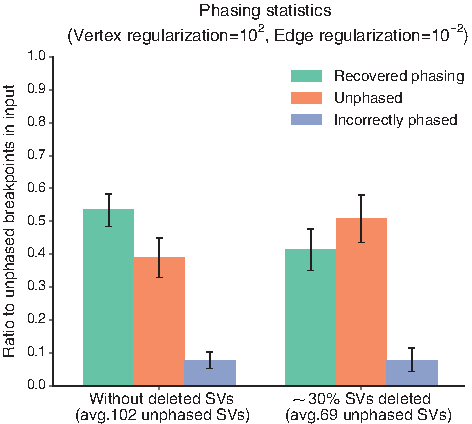
Under these parameters, we present the phasing results in Figure 2. If we have the entire set of possible SVs, over 50% of the \documentclass{aastex}\usepackage{amsbsy}\usepackage{amsfonts}\usepackage{amssymb}\usepackage{bm}\usepackage{mathrsfs}\usepackage{pifont}\usepackage{stmaryrd}\usepackage{textcomp}\usepackage{portland, xspace}\usepackage{amsmath, amsxtra}\usepackage{upgreek}\pagestyle{empty}\DeclareMathSizes{10}{9}{7}{6}\begin{document}
$$\sim$$
\end{document}100 unphased SVs are correctly phased, while the number of incorrectly phased SVs is quite low (\documentclass{aastex}\usepackage{amsbsy}\usepackage{amsfonts}\usepackage{amssymb}\usepackage{bm}\usepackage{mathrsfs}\usepackage{pifont}\usepackage{stmaryrd}\usepackage{textcomp}\usepackage{portland, xspace}\usepackage{amsmath, amsxtra}\usepackage{upgreek}\pagestyle{empty}\DeclareMathSizes{10}{9}{7}{6}\begin{document}
$$< 10$$
\end{document}%). However, a large number of SVs may remain unphased, that is, more than 1 possible phasing is predicted for them. If we do not detect \documentclass{aastex}\usepackage{amsbsy}\usepackage{amsfonts}\usepackage{amssymb}\usepackage{bm}\usepackage{mathrsfs}\usepackage{pifont}\usepackage{stmaryrd}\usepackage{textcomp}\usepackage{portland, xspace}\usepackage{amsmath, amsxtra}\usepackage{upgreek}\pagestyle{empty}\DeclareMathSizes{10}{9}{7}{6}\begin{document}
$$\sim$$
\end{document}30% of the SVs that occurred, the noise added causes the quality of the phasing to drop significantly, and the mean percentage of correctly phased SVs drops to about 40%. The number of incorrectly phased SVs remains under 10%, which means the method does not create many false positives and is quite specific, but in the absence of nonlinearity, the number of unphased SVs remains high.
Phasing results for the two different simulation sets we create. Both sets consist of approximately the same number of genomic regions as the HeLa results produced by Weaver (Li et al., 2016). In the first one, we keep all the simulated SVs, but discard the phasing of breakpoints with probability about 0.30. This leads to \documentclass{aastex}\usepackage{amsbsy}\usepackage{amsfonts}\usepackage{amssymb}\usepackage{bm}\usepackage{mathrsfs}\usepackage{pifont}\usepackage{stmaryrd}\usepackage{textcomp}\usepackage{portland, xspace}\usepackage{amsmath, amsxtra}\usepackage{upgreek}\pagestyle{empty}\DeclareMathSizes{10}{9}{7}{6}\begin{document}
$$\sim$$
\end{document}102 unphased SVs, of which we can correctly phase \documentclass{aastex}\usepackage{amsbsy}\usepackage{amsfonts}\usepackage{amssymb}\usepackage{bm}\usepackage{mathrsfs}\usepackage{pifont}\usepackage{stmaryrd}\usepackage{textcomp}\usepackage{portland, xspace}\usepackage{amsmath, amsxtra}\usepackage{upgreek}\pagestyle{empty}\DeclareMathSizes{10}{9}{7}{6}\begin{document}
$$\sim$$
\end{document}52%. In the second set, we also delete SVs with probability 0.30, leading to \documentclass{aastex}\usepackage{amsbsy}\usepackage{amsfonts}\usepackage{amssymb}\usepackage{bm}\usepackage{mathrsfs}\usepackage{pifont}\usepackage{stmaryrd}\usepackage{textcomp}\usepackage{portland, xspace}\usepackage{amsmath, amsxtra}\usepackage{upgreek}\pagestyle{empty}\DeclareMathSizes{10}{9}{7}{6}\begin{document}
$$\sim$$
\end{document}69 SVs on average. In this case, the missing information from the deleted breakpoints affects the phasing inference, and the number of recovered SVs that are phased correctly is fewer than those that remain unphased. In both cases, however, the number of wrongly phased SVs is only \documentclass{aastex}\usepackage{amsbsy}\usepackage{amsfonts}\usepackage{amssymb}\usepackage{bm}\usepackage{mathrsfs}\usepackage{pifont}\usepackage{stmaryrd}\usepackage{textcomp}\usepackage{portland, xspace}\usepackage{amsmath, amsxtra}\usepackage{upgreek}\pagestyle{empty}\DeclareMathSizes{10}{9}{7}{6}\begin{document}
$$\sim$$
\end{document}8%.
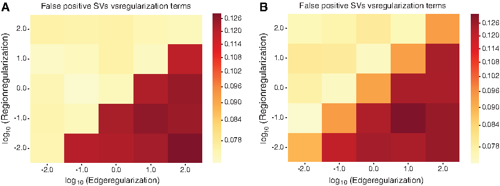
Figure 3 shows how the number of incorrectly phased SVs, that is, false positives, in the two simulation data sets varies as the two regularization parameters are changed. We note that the number of incorrectly phased SVs is always quite low, at \documentclass{aastex}\usepackage{amsbsy}\usepackage{amsfonts}\usepackage{amssymb}\usepackage{bm}\usepackage{mathrsfs}\usepackage{pifont}\usepackage{stmaryrd}\usepackage{textcomp}\usepackage{portland, xspace}\usepackage{amsmath, amsxtra}\usepackage{upgreek}\pagestyle{empty}\DeclareMathSizes{10}{9}{7}{6}\begin{document}
$$\le$$
\end{document}15% of the number of unphased SVs in the input. Indeed, assuming all SVs are detected, then with reasonable parameter values the number of errors during phasing can be kept to single digits. However, if the regularization coefficient for the edges exceeds that used for regions, the quality of the phasing drops significantly in both data sets. This is expected behavior, considering that the number of errors in ASCNs of regions is significantly lower than that for edges. Therefore, if the ASCNS is perturbed and we have to find the phasing, it is more likely to introduce errors by disallowing large corrections in the ASCNS than by disallowing large corrections in the ASCNG.
Variation in the number of incorrectly phased SVs with variation in the two regularization terms. The weighting coefficient is kept constant at 1. The axes are log scaled.
4.2. Application to the HeLa whole-genome sequencing data
To evaluate the method on real data, we used as input, noisy results from Weaver on the HeLa whole-genome sequencing data set (Li et al., 2016) on the HeLa genome (Adey et al., 2013). In this input, we examined the results for our method when the number of phased breakpoints is varied. We then verified how our recovered phasing compares with the prediction from Weaver, and how it is affected when noise is introduced in the form of perturbation in the copy numbers of the SVs and the regions.
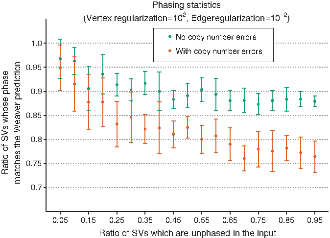
Figure 4 shows the fraction of SVs where our phasing prediction is similar to that predicted by Weaver versus the fraction of unphased SVs in the input. The results were calculated at parameter values of \documentclass{aastex}\usepackage{amsbsy}\usepackage{amsfonts}\usepackage{amssymb}\usepackage{bm}\usepackage{mathrsfs}\usepackage{pifont}\usepackage{stmaryrd}\usepackage{textcomp}\usepackage{portland, xspace}\usepackage{amsmath, amsxtra}\usepackage{upgreek}\pagestyle{empty}\DeclareMathSizes{10}{9}{7}{6}\begin{document}
$$\ell , \;100 \ell , \;.01$$
\end{document} for the cost, region regularization, and edge regularization parameters, respectively, where \documentclass{aastex}\usepackage{amsbsy}\usepackage{amsfonts}\usepackage{amssymb}\usepackage{bm}\usepackage{mathrsfs}\usepackage{pifont}\usepackage{stmaryrd}\usepackage{textcomp}\usepackage{portland, xspace}\usepackage{amsmath, amsxtra}\usepackage{upgreek}\pagestyle{empty}\DeclareMathSizes{10}{9}{7}{6}\begin{document}
$$\ell$$
\end{document} is the length of the corresponding region. In the results obtained, we found that our method manages to recover a large percentage of discarded phasing information. When the copy numbers of the regions and the SVs are known, we can recover almost 90% or better of the predicted phasing by Weaver, irrespective of the number of SVs that are already phased. Weaver, on the contrary, uses germ line SNP data and their haplotype information from the 1000 Genomes Project to predict phasing.
Phasing results compared to Weaver on the HeLa whole-genome sequencing data. The x-axis represents the fraction of unphased SVs in the input provided to our method, while the y-axis is the fraction of SVs where the recovered phasing agrees with that obtained by Weaver. The green plot shows the results when the input does not have noisy copy numbers, which should aid phasing. The orange plot shows how the results vary when copy numbers of SVs and regions are perturbed with probability 0.3.
When noise is introduced, the fraction of recovered phasing drops to \documentclass{aastex}\usepackage{amsbsy}\usepackage{amsfonts}\usepackage{amssymb}\usepackage{bm}\usepackage{mathrsfs}\usepackage{pifont}\usepackage{stmaryrd}\usepackage{textcomp}\usepackage{portland, xspace}\usepackage{amsmath, amsxtra}\usepackage{upgreek}\pagestyle{empty}\DeclareMathSizes{10}{9}{7}{6}\begin{document}
$$\sim$$
\end{document}74% when only 5% of the original input is phased, but it rises to \documentclass{aastex}\usepackage{amsbsy}\usepackage{amsfonts}\usepackage{amssymb}\usepackage{bm}\usepackage{mathrsfs}\usepackage{pifont}\usepackage{stmaryrd}\usepackage{textcomp}\usepackage{portland, xspace}\usepackage{amsmath, amsxtra}\usepackage{upgreek}\pagestyle{empty}\DeclareMathSizes{10}{9}{7}{6}\begin{document}
$$\sim$$
\end{document}90% if even 50% of the original input is phased. Therefore, any noise in the copy number data is being offset by prior information about the phasing of some SVs. This information allows the method to balance some of the copy numbers so that the phasing of the remaining SVs can be recovered. In Figure 5, we provide an example of an SV in a region with CNAs in the HeLa data, where the predicted phase is consistent with the Weaver prediction. Note that the prediction is unaffected by other unphased SVs (not shown in the figure) in a region with a large number of CNAs.
(A) A Genome Browser view that shows two possible phasings of a given SV (a deletion) in the HeLa genome, where the phasing prediction by Weaver was discarded, in a region with a large number of unphased SVs and CNAs. The number of CNAs and SVs makes it liable to predict the phasing incorrectly. The two tracks represent allele A and allele B frequencies for regions on chromosome 11 as predicted by Weaver. The red edges are possible phasings of an SV detected on the chromosome. On solving (3), one of these possibilities is predicted to have copy number 0 (dotted edge), and the other (solid edge), which is the phasing predicted by Weaver, has copy number 2. Note that other unphased SVs in the figure are not shown for clarity. (B) A schematic representation of the corresponding incomplete allele-specific cancer genome graph near the region shown in (A). Here the regions are represented as oriented blocks, with the number on each block referring to their ASCNG. The green connections represent a large set of regions excluded in the schematic. These regions are also subject to unrepresented SVs that may have confounded the inference. Despite this, the inference agrees with Weaver's prediction, which was erased from the input. ASCNG, allele-specific copy numbers of genomic regions; CNAs, copy number alterations.
4.3. Application to ovarian cancer data from TCGA
In Li et al. (2016), Weaver was used to infer allele-specific copy numbers and phasing information for TCGA ovarian cancer samples. The number of SVs detected in these samples varied from under 50 to over 500. However, on average, 23% of the SVs detected in a sample were unphased, and some of the detected unphased variants were inferred to have copy number 0. Some samples had over 50% of the detected SVs unphased at either one or both breakpoints. We attempted to resolve these variants using the convex programming framework introduced in this article, and classified the SVs into three classes: (1) variants that were phased using the framework and were estimated to have nonzero copy number; (2) variants that remained unphased; and (3) variants whose copy number is predicted to be 0 by both Weaver and the ILP.
In these results, summarized in Table 1, about 60% on average of the unphased SVs in the samples were estimated to have a copy number of 0, matching the estimation through Weaver. We classify these as undetermined variants, since we cannot distinguish the classes they might fall into, nor the phasing. However, of the other 40% of the SVs that are predicted to have nonzero copy number, almost 60% are phased on average, with the number of ambiguous phasings never rising above single digits. Thus, for a large number of SVs with predicted copy number \documentclass{aastex}\usepackage{amsbsy}\usepackage{amsfonts}\usepackage{amssymb}\usepackage{bm}\usepackage{mathrsfs}\usepackage{pifont}\usepackage{stmaryrd}\usepackage{textcomp}\usepackage{portland, xspace}\usepackage{amsmath, amsxtra}\usepackage{upgreek}\pagestyle{empty}\DeclareMathSizes{10}{9}{7}{6}\begin{document}
$$> 0$$
\end{document}, we are able to obtain a single, unambiguous phasing.
The Results of the Integer Linear Program on 36 Ovarian Cancer Samples from The Cancer Genome Atlas (TCGA)
Sample name
SVs detected by weaver
Unphased SVs
Newly phased SVs
Remaining unphased SVs
Undetermined SVs
TCGA-04-1331
80
24
10
3
11
TCGA-04-1347
174
25
11
5
9
TCGA-04-1349
62
7
3
1
3
TCGA-04-1367
59
24
4
2
18
TCGA-04-1514
173
73
14
7
52
TCGA-09-1666
222
105
21
8
76
TCGA-09-2045
105
14
4
2
8
TCGA-09-2050
120
21
3
6
12
TCGA-10-0934
128
7
0
2
5
TCGA-10-0937
100
17
6
2
9
TCGA-10-0938
276
89
18
7
64
TCGA-13-0725
21
8
2
2
4
TCGA-13-0751
120
19
6
5
8
TCGA-13-0906
94
22
1
6
15
TCGA-13-1477
17
6
2
1
3
TCGA-13-1487
275
29
5
5
19
TCGA-13-1491
101
19
4
1
14
TCGA-23-1110
145
32
7
5
20
TCGA-24-0982
32
8
2
4
2
TCGA-24-1419
51
10
4
1
5
TCGA-24-1466
527
39
16
9
14
TCGA-24-1544
288
152
13
7
132
TCGA-24-1548
73
9
2
2
5
TCGA-24-1557
265
37
8
4
25
TCGA-24-1558
189
26
8
3
15
TCGA-24-1562
92
11
4
1
6
TCGA-24-1614
180
80
11
9
60
TCGA-24-2024
67
19
1
3
15
TCGA-24-2290
168
55
10
4
41
TCGA-25-1632
165
11
2
2
7
TCGA-25-1634
118
28
8
8
12
TCGA-25-2391
88
24
2
3
19
TCGA-25-2400
213
54
29
6
19
TCGA-36-1570
161
29
7
6
16
TCGA-36-1574
114
21
9
3
9
TCGA-61-2000
460
90
13
3
74
The first column gives the sample ID. The second column shows the number of the SVs identified by Weaver, while the third column shows the number of SVs that are left unphased. The fourth column shows the number of SVs that are phased by the ILP and are predicted to have more than 1 copy. The fifth column is the number of SVs whose phase is left ambiguous by the ILP, although Weaver predicts that they have nonzero copies. The sixth and final column shows the number of SVs that are predicted to have copy number 0 by both Weaver and the ILP. These are classified as undetermined SVs.
SV, structural variants.
5. Discussion and Conclusion
The main contribution of this article is a combinatorial framework within which we can examine allele-specific rearrangements in cancer genomes. An advantage of our method is that given ASCN information and putative SVs from any source, we can infer phased SVs efficiently. We showed that this framework, as implemented here, has high specificity. As a proof-of-principle, we demonstrated the performance of our method on real data. Even in the presence of external noise in the form of errors in the input ASCNs, our results agreed closely with the original predicted results from Weaver that used many other types of input data (germ line SNP and read linkage from paired-end reads) to obtain SV phasing information.
The method proposed in this article can also be extended for more sophisticated inference. We will explore adding further nonlinear constraints that can capture information gathered from long-range sequencing and alignment data, such as PacBio and 10 × Genomics data. In such a framework, we should be able to incorporate both long and short read data into a comprehensive assembly-like problem formulation and obtain a description of the cancer genome through the cancer genome graph. In addition, a theoretical analysis of the method, in the sense of accuracy of rounded solutions to relaxations of problem, can also be pursued. Assuming we can bind the error in our prediction of value of the objective function, we believe the main drawback in the current iteration of the method, which is the number of false negatives, can be overcome.
We also do not specifically consider the problem of subclones in this work. Indeed, if multiple clones are present, then the incomplete allele-specific cancer genome graph obtained will represent SVs from different subclones, and the problem of decomposing the graph into individual clones needs to be addressed. Finally, from a practical point of view, the ILP framework is fast and efficient for most cases, but there is no guarantee of a polynomial time solution. For certain input programs, for example, the algorithm may take exponential time, and it is hard to quantify which cases these are. In the context of the large graphs being handled, this could be a potential problem. A more thorough analysis, a more efficient implementation, and a study of the structure of edge cases would improve the utility of the method.
Footnotes
Acknowledgments
The authors thank the anonymous reviewers for suggestions that improved the article. The authors also thank the TCGA Research Network for making the data publicly available. This work is supported, in part, by the National Institutes of Health Grants CA182360 and HG007352 (to J.M.), and the National Science Foundation Grants 1054309 and 1262575 (to J.M.).
Author Disclosure Statement
No competing financial interests exist.
References
1.
AdeyA., BurtonJ.N., KitzmanJ.O., et al.2013. The haplotype-resolved genome and epigenome of the aneuploid hela cancer cell line. Nature, 500, 207–211.
2.
BeroukhimR., MermelC.H., PorterD., et al.2010. The landscape of somatic copy-number alteration across human cancers. Nature, 463, 899–905.
3.
CarterS.L., CibulskisK., HelmanE., et al.2012. Absolute quantification of somatic DNA alterations in human cancer. Nat. Biotechnol. 30, 413–421.
4.
CarvalhoC.M., and LupskiJ.R.2016. Mechanisms underlying structural variant formation in genomic disorders. Nat. Rev. Genet. 17, 224–238.
5.
DiamondS., and BoydS.2016. CVXPY: A python-embedded modeling language for convex optimization. J. Mach. Learn. Res. 17, 1–5.
6.
DzambaM., RamaniA.K., BuczkowiczP., et al.2017. Identification of complex genomic rearrangements in cancers using CouGaR. Genome Res. 27, 107–117.
7.
EidJ., FehrA., GrayJ., et al.2009. Real-time DNA sequencing from single polymerase molecules. Science, 323, 133–138.
8.
GordonD.J., ResioB., and PellmanD.2012. Causes and consequences of aneuploidy in cancer. Nat. Rev. Genet. 13, 189–203.
9.
GreenmanC.D., PleasanceE.D., NewmanS., et al., 2012. Estimation of rearrangement phylogeny for cancer genomes. Genome Res. 22, 346–361.
10.
GuptaA., PlaceM., GoldsteinS., et al.2015. Single-molecule analysis reveals widespread structural variation in multiple myeloma. Proc. Natl Acad. Sci. U. S. A., 112, 7689–7694.
KarpR.M.1972. Reducibility among combinatorial problems, 85–103. In Complexity of Computer Computations. Eds: MillerR.E., TatcherJ.W., BohlingerJ.D.Springer; Boston, MA.
13.
KimuraM.1969. The number of heterozygous nucleotide sites maintained in a finite population due to steady flux of mutations. Genetics, 61, 893.
14.
LiY., ZhouS., SchwartzD.C., et al.2016. Allele-specific quantification of structural variations in cancer genomes. Cell Syst. 3, 21–34.
15.
MaJ., RatanA., RaneyB.J., et al.2008. The infinite sites model of genome evolution. Proc. Natl Acad. Sci. U. S. A., 105, 14254–14261.
16.
MedvedevP., FiumeM., DzambaM., et al.2010. Detecting copy number variation with mated short reads. Genome Res. 20, 1613–1622.
17.
MedvedevP., StanciuM., and BrudnoM.2009. Computational methods for discovering structural variation with next-generation sequencing. Nat. Methods, 6, S13–S20.
18.
OesperL., RitzA., AerniS.J., et al.2012. Reconstructing cancer genomes from paired-end sequencing data. BMC Bioinformatics, 13, S10.
19.
Van LooP., NordgardS.H., LingjærdeO.C., et al.2010. Allele-specific copy number analysis of tumors. Proc. Natl Acad. Sci. U. S. A., 107, 16910–16915.
20.
WangJ., MullighanC.G., EastonJ., et al.2011. Crest maps somatic structural variation in cancer genomes with base-pair resolution. Nat. Methods. 8, 652–654.
21.
ZackT.I., SchumacherS.E., CarterS.L., et al.2013. Pan-cancer patterns of somatic copy number alteration. Nat. Genet. 45, 1134–1140.
22.
ZerbinoD.R., BallingerT., PatenB., et al.2016. Representing and decomposing genomic structural variants as balanced integer flows on sequence graphs. BMC Bioinformatics. 17, 400.
23.
ZhengG.X., LauB.T., Schnall-LevinM., et al.2016. Haplotyping germline and cancer genomes with high-throughput linked-read sequencing. Nat. Biotechnol. 34, 303–311.