Structure-Aware Principal Component Analysis for Single-Cell RNA-seq Data

Abstract

With the emergence of droplet-based technologies, it has now become possible to profile transcriptomes of several thousands of cells in a day. Although such a large single-cell cohort may favor the discovery of cellular heterogeneity, it also brings new challenges in the prediction of minority cell types. Identification of any minority cell type holds a special significance in knowledge discovery. In the analysis of single-cell expression data, the use of principal component analysis (PCA) is surprisingly frequent for dimension reduction. The principal directions obtained from PCA are usually dominated by the major cell types in the concerned tissue. Thus, it is very likely that using a traditional PCA may endanger the discovery of minority populations. To this end, we propose locality-sensitive PCA (LSPCA), a scalable variant of PCA equipped with structure-aware data sampling at its core. Structure-aware sampling provides PCA with a neutral spread of the data, thereby reducing the bias in its principal directions arising from the redundant samples in a data set. We benchmarked the performance of the proposed method on ten publicly available single-cell expression data sets including one very large annotated data set. Results have been compared with traditional PCA and PCA with random sampling. Clustering results on the annotated data sets also show that LSPCA can detect the minority populations with a higher accuracy.

1. Introduction

Recently, Macosko et al. (2015) introduced droplet-based bar-coding technology that allows RNA sequencing of single cells (sc-RNAseq) at a massive scale producing large data sets. The sample size of the sc-RNAseq data sets has skyrocketed from 18 samples (2012) to 1.3 million samples (Wagner et al., 2016). A key promise of single-cell technology is to uncover the cellular heterogeneity within a tissue through transcriptomic analysis (Shalek et al., 2013). The subpopulations may exist in large numbers or as minor (rare) groups. The challenge to discover these minor subpopulations from the large cohort is nontrivial (Grün et al., 2015).

Principal component analysis (PCA) is widely used as a dimension reduction tool when investigating a transcriptome data set. Owing to the mechanics of PCA, for a sc-RNAseq data set with typically ∼25K genes and a few hundreds to thousands of samples, the principal directions obtained from a traditional PCA is likely to be biased by the larger groups in the data set. To put it simply, the top principal components are dominated by the sheer number of data points in larger groups, thereby superseding the effect of small subpopulations. This poses a major setback in the analysis of sc-RNAseq data sets.

Inspired by the benefits of sampling in imbalanced data sets (Chawla et al., 2002; Martinsson et al., 2011), we propose to improvise PCA by introducing a systematic down-sampling step before PCA. We identify this step as the structure-aware data sampling. To this end, we have built a scalable dimension reduction framework—locality-sensitive principal component analysis (LSPCA).

We evaluated LSPCA on multiple single-cell data sets including a large data set of ∼68K peripheral blood mononuclear cell (PBMC) transcriptomes, where the true cell type annotations were available. When evaluating the clustering outcome on the annotated data set using LSPCA, we obtained better adjusted Rand index (ARI) than classic PCA. As a noteworthy benefit of LSPCA, we also observed that LSPCA performs better in discovering the minority cell groups. Besides that, we validated on nine unannotated data sets, that the principal components resulting from LSPCA are more identical to classic PCA components than to the randomized variant of PCA (Martinsson et al., 2011). Details of the results on all data sets are discussed in Section 6.

2. Background

2.1. Locality-sensitive hashing

Locality-sensitive hashing (LSH) (Indyk et al., 1997; Pauleve et al., 2010; Leskovec et al., 2014) operates on a reduced dimension to find approximate nearest neighbors. LSH uses special locality-sensitive hash functions where the chances of similar objects hashing into a same bucket are more than the collision of dissimilar objects (Bawa et al., 2005).

Each hash function projects a sample point on one random hyperplane and returns a Boolean value. The Boolean value corresponds to a sign (0/1) depending on which side of the hyperplane the projected point lies. By concatenating the output from multiple such hash functions, a string of Boolean values is derived for the corresponding sample. Unique hash strings encode for bucket identifiers that represent boundaries of neighborhood called “regions.” During search, a bucket identifier of the query object is generated using the same set of hash functions. Only the members within a region, called “candidates,” are used to compute for actual similarity. The approximate nearest neighbors are searched within and around the given query object region, which reduces the computation time for n query points from \documentclass{aastex}\usepackage{amsbsy}\usepackage{amsfonts}\usepackage{amssymb}\usepackage{bm}\usepackage{mathrsfs}\usepackage{pifont}\usepackage{stmaryrd}\usepackage{textcomp}\usepackage{portland, xspace}\usepackage{amsmath, amsxtra}\usepackage{upgreek}\pagestyle{empty}\DeclareMathSizes{10}{9}{7}{6}\begin{document} $${ \cal O} ( {n^2} )$$ \end{document} to \documentclass{aastex}\usepackage{amsbsy}\usepackage{amsfonts}\usepackage{amssymb}\usepackage{bm}\usepackage{mathrsfs}\usepackage{pifont}\usepackage{stmaryrd}\usepackage{textcomp}\usepackage{portland, xspace}\usepackage{amsmath, amsxtra}\usepackage{upgreek}\pagestyle{empty}\DeclareMathSizes{10}{9}{7}{6}\begin{document} $${ \cal O} ( n \log n )$$ \end{document} .

The performance of the LSH method depends on the choice of a few parameters such as the distance metric between neighbors, number of hash functions, and the number of hash tables. Choosing of these parameters is a nontrivial task that is addressed in an advanced self-tuning version of LSH known as LSHForest (Bawa et al., 2005). We have used the LSHForest for the sampling process in the proposed algorithm.

2.2. Principal component analysis

PCA (Karamizadeh et al., 2013) is a statistical technique that converts the observation points of correlated variables to linearly uncorrelated variables using orthogonal transformations. PCA is widely used as a dimension reduction technique (Li et al., 2008). Mathematically, PCA is defined as an orthogonal linear transformation of data into a new coordinate system by iteratively projecting instances on the direction of maximum variance (Jolliffe, 1986). PCA of a data matrix \documentclass{aastex}\usepackage{amsbsy}\usepackage{amsfonts}\usepackage{amssymb}\usepackage{bm}\usepackage{mathrsfs}\usepackage{pifont}\usepackage{stmaryrd}\usepackage{textcomp}\usepackage{portland, xspace}\usepackage{amsmath, amsxtra}\usepackage{upgreek}\pagestyle{empty}\DeclareMathSizes{10}{9}{7}{6}\begin{document} $${{ \bf{X}}_{n \times m}}$$ \end{document} may be performed by diagonalizing its corresponding covariance matrix (a symmetric matrix) to obtain \documentclass{aastex}\usepackage{amsbsy}\usepackage{amsfonts}\usepackage{amssymb}\usepackage{bm}\usepackage{mathrsfs}\usepackage{pifont}\usepackage{stmaryrd}\usepackage{textcomp}\usepackage{portland, xspace}\usepackage{amsmath, amsxtra}\usepackage{upgreek}\pagestyle{empty}\DeclareMathSizes{10}{9}{7}{6}\begin{document} $${{ \bf{E}}_{m \times m}}$$ \end{document} . The diagonal matrix consists of eigenvalues in decreasing order on the diagonal. The eigenvectors are called principal axes or principal directions of the data.

Singular value decomposition (SVD) is a matrix factorization method providing a robust computational framework to compute the principal components accurately for a variety of data sets. It is the generalization of the eigen decomposition. It is used to obtain \documentclass{aastex}\usepackage{amsbsy}\usepackage{amsfonts}\usepackage{amssymb}\usepackage{bm}\usepackage{mathrsfs}\usepackage{pifont}\usepackage{stmaryrd}\usepackage{textcomp}\usepackage{portland, xspace}\usepackage{amsmath, amsxtra}\usepackage{upgreek}\pagestyle{empty}\DeclareMathSizes{10}{9}{7}{6}\begin{document} $$d = k < m$$ \end{document} principal components without the need to compute the diagonal matrix of the whole covariance matrix, which also overcomes the restrictions caused by ill-conditioned matrices.

The steps to transform the original matrix into the new space are enumerated hereunder.

Construct the covariance matrix, \documentclass{aastex}\usepackage{amsbsy}\usepackage{amsfonts}\usepackage{amssymb}\usepackage{bm}\usepackage{mathrsfs}\usepackage{pifont}\usepackage{stmaryrd}\usepackage{textcomp}\usepackage{portland, xspace}\usepackage{amsmath, amsxtra}\usepackage{upgreek}\pagestyle{empty}\DeclareMathSizes{10}{9}{7}{6}\begin{document} $${ \bf{CV}}$$ \end{document} , of the mean centered data.

Compute the eigenvalue matrix ( \documentclass{aastex}\usepackage{amsbsy}\usepackage{amsfonts}\usepackage{amssymb}\usepackage{bm}\usepackage{mathrsfs}\usepackage{pifont}\usepackage{stmaryrd}\usepackage{textcomp}\usepackage{portland, xspace}\usepackage{amsmath, amsxtra}\usepackage{upgreek}\pagestyle{empty}\DeclareMathSizes{10}{9}{7}{6}\begin{document} $${{ \bf{{ E}}}_{m \times m}}$$ \end{document} ) of \documentclass{aastex}\usepackage{amsbsy}\usepackage{amsfonts}\usepackage{amssymb}\usepackage{bm}\usepackage{mathrsfs}\usepackage{pifont}\usepackage{stmaryrd}\usepackage{textcomp}\usepackage{portland, xspace}\usepackage{amsmath, amsxtra}\usepackage{upgreek}\pagestyle{empty}\DeclareMathSizes{10}{9}{7}{6}\begin{document} $${ \bf{CV}}$$ \end{document} .

Compute \documentclass{aastex}\usepackage{amsbsy}\usepackage{amsfonts}\usepackage{amssymb}\usepackage{bm}\usepackage{mathrsfs}\usepackage{pifont}\usepackage{stmaryrd}\usepackage{textcomp}\usepackage{portland, xspace}\usepackage{amsmath, amsxtra}\usepackage{upgreek}\pagestyle{empty}\DeclareMathSizes{10}{9}{7}{6}\begin{document} $${ \bf{E ^\prime }}$$ \end{document} by sorting \documentclass{aastex}\usepackage{amsbsy}\usepackage{amsfonts}\usepackage{amssymb}\usepackage{bm}\usepackage{mathrsfs}\usepackage{pifont}\usepackage{stmaryrd}\usepackage{textcomp}\usepackage{portland, xspace}\usepackage{amsmath, amsxtra}\usepackage{upgreek}\pagestyle{empty}\DeclareMathSizes{10}{9}{7}{6}\begin{document} $${ \bf{E}}$$ \end{document} according to its corresponding eigenvalues in decreasing order.

Transform \documentclass{aastex}\usepackage{amsbsy}\usepackage{amsfonts}\usepackage{amssymb}\usepackage{bm}\usepackage{mathrsfs}\usepackage{pifont}\usepackage{stmaryrd}\usepackage{textcomp}\usepackage{portland, xspace}\usepackage{amsmath, amsxtra}\usepackage{upgreek}\pagestyle{empty}\DeclareMathSizes{10}{9}{7}{6}\begin{document} $${ \bf{X}}$$ \end{document} to \documentclass{aastex}\usepackage{amsbsy}\usepackage{amsfonts}\usepackage{amssymb}\usepackage{bm}\usepackage{mathrsfs}\usepackage{pifont}\usepackage{stmaryrd}\usepackage{textcomp}\usepackage{portland, xspace}\usepackage{amsmath, amsxtra}\usepackage{upgreek}\pagestyle{empty}\DeclareMathSizes{10}{9}{7}{6}\begin{document} $${ \bf{PC}}$$ \end{document} by projecting \documentclass{aastex}\usepackage{amsbsy}\usepackage{amsfonts}\usepackage{amssymb}\usepackage{bm}\usepackage{mathrsfs}\usepackage{pifont}\usepackage{stmaryrd}\usepackage{textcomp}\usepackage{portland, xspace}\usepackage{amsmath, amsxtra}\usepackage{upgreek}\pagestyle{empty}\DeclareMathSizes{10}{9}{7}{6}\begin{document} $${ \bf{X}}$$ \end{document} on \documentclass{aastex}\usepackage{amsbsy}\usepackage{amsfonts}\usepackage{amssymb}\usepackage{bm}\usepackage{mathrsfs}\usepackage{pifont}\usepackage{stmaryrd}\usepackage{textcomp}\usepackage{portland, xspace}\usepackage{amsmath, amsxtra}\usepackage{upgreek}\pagestyle{empty}\DeclareMathSizes{10}{9}{7}{6}\begin{document} $${ \bf{E ^\prime }}$$ \end{document} .

Note that the first principal component of \documentclass{aastex}\usepackage{amsbsy}\usepackage{amsfonts}\usepackage{amssymb}\usepackage{bm}\usepackage{mathrsfs}\usepackage{pifont}\usepackage{stmaryrd}\usepackage{textcomp}\usepackage{portland, xspace}\usepackage{amsmath, amsxtra}\usepackage{upgreek}\pagestyle{empty}\DeclareMathSizes{10}{9}{7}{6}\begin{document} $${{ \bf{x}}_{{ \bf{ ( i ) }}}}$$ \end{document} in the transformed co-ordinates is given by \documentclass{aastex}\usepackage{amsbsy}\usepackage{amsfonts}\usepackage{amssymb}\usepackage{bm}\usepackage{mathrsfs}\usepackage{pifont}\usepackage{stmaryrd}\usepackage{textcomp}\usepackage{portland, xspace}\usepackage{amsmath, amsxtra}\usepackage{upgreek}\pagestyle{empty}\DeclareMathSizes{10}{9}{7}{6}\begin{document} \begin{align*} { \bf{P}}{{ \bf{C}}_{ \bf{1}}} = { \bf{X}} \cdot {{ \bf{E ^\prime }}_{ ( 1 ) }} , \end{align*} \end{document}

where \documentclass{aastex}\usepackage{amsbsy}\usepackage{amsfonts}\usepackage{amssymb}\usepackage{bm}\usepackage{mathrsfs}\usepackage{pifont}\usepackage{stmaryrd}\usepackage{textcomp}\usepackage{portland, xspace}\usepackage{amsmath, amsxtra}\usepackage{upgreek}\pagestyle{empty}\DeclareMathSizes{10}{9}{7}{6}\begin{document} $${{ \bf{E ^\prime }}_{ ( k ) }} = ( {E ^\prime _1} , \ldots , {E ^\prime _m}{ ) _{ ( k ) }}$$ \end{document} , \documentclass{aastex}\usepackage{amsbsy}\usepackage{amsfonts}\usepackage{amssymb}\usepackage{bm}\usepackage{mathrsfs}\usepackage{pifont}\usepackage{stmaryrd}\usepackage{textcomp}\usepackage{portland, xspace}\usepackage{amsmath, amsxtra}\usepackage{upgreek}\pagestyle{empty}\DeclareMathSizes{10}{9}{7}{6}\begin{document} $$k = 1 , \ldots m$$ \end{document} , is a unit vector of weights that transforms each row vector \documentclass{aastex}\usepackage{amsbsy}\usepackage{amsfonts}\usepackage{amssymb}\usepackage{bm}\usepackage{mathrsfs}\usepackage{pifont}\usepackage{stmaryrd}\usepackage{textcomp}\usepackage{portland, xspace}\usepackage{amsmath, amsxtra}\usepackage{upgreek}\pagestyle{empty}\DeclareMathSizes{10}{9}{7}{6}\begin{document} $${{ \bf{x}}_{{ \bf{ ( i ) }}}}$$ \end{document} of \documentclass{aastex}\usepackage{amsbsy}\usepackage{amsfonts}\usepackage{amssymb}\usepackage{bm}\usepackage{mathrsfs}\usepackage{pifont}\usepackage{stmaryrd}\usepackage{textcomp}\usepackage{portland, xspace}\usepackage{amsmath, amsxtra}\usepackage{upgreek}\pagestyle{empty}\DeclareMathSizes{10}{9}{7}{6}\begin{document} $${ \bf{X}}$$ \end{document} to a new vector of principal component scores \documentclass{aastex}\usepackage{amsbsy}\usepackage{amsfonts}\usepackage{amssymb}\usepackage{bm}\usepackage{mathrsfs}\usepackage{pifont}\usepackage{stmaryrd}\usepackage{textcomp}\usepackage{portland, xspace}\usepackage{amsmath, amsxtra}\usepackage{upgreek}\pagestyle{empty}\DeclareMathSizes{10}{9}{7}{6}\begin{document} $${ \bf{P}}{{ \bf{C}}_{ ( k ) }} = ( P{C_1} , \ldots , P{C_d}{ ) _{ ( k ) }}$$ \end{document} , where \documentclass{aastex}\usepackage{amsbsy}\usepackage{amsfonts}\usepackage{amssymb}\usepackage{bm}\usepackage{mathrsfs}\usepackage{pifont}\usepackage{stmaryrd}\usepackage{textcomp}\usepackage{portland, xspace}\usepackage{amsmath, amsxtra}\usepackage{upgreek}\pagestyle{empty}\DeclareMathSizes{10}{9}{7}{6}\begin{document} $${ \bf{P}}{{ \bf{C}}_{ \bf{k}}}$$ \end{document} denotes the kth principal component.

3. Data Preprocessing

Data sets containing raw unique molecular identifier (UMI) read counts were downloaded from multiple sources: (1) using the Bioconductor recount package by Collado-Torres et al. (2017), (2) from the www.support.10xgenomics.com website, and (3) the adult and fetal human brain scRNA-seq data set by Darmanis et al. (2015). Each data set was preprocessed using the steps outlined in Figure 1.

Cell and gene filtering: Raw count matrix was filtered for poor quality cells. Typically single-cell data sets have >20,000 genes. Genes having count >2 in at least four cells were kept for subsequent preprocessing.

Median normalization: The filtered data matrix was median normalized. The median normalization step then involved division of UMI counts in the filtered matrix by the total UMI counts in each cell. These scaled counts were multiplied by the median of the total UMI counts across cells (Zheng et al., 2017).

Gene selection: To select the top dispersed genes, 2000 most variable genes were selected based on their relative dispersion (variance/mean) with respect to the expected dispersion across genes with similar average expression (Macosko et al., 2015; Zheng et al., 2017).

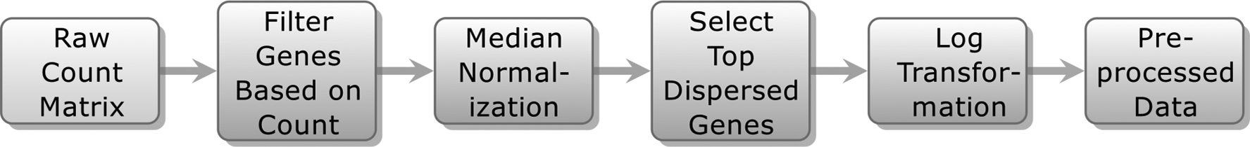
Log normalization: The resulting matrix (of dimension n cells × 2000 genes) was further subjected to \documentclass{aastex}\usepackage{amsbsy}\usepackage{amsfonts}\usepackage{amssymb}\usepackage{bm}\usepackage{mathrsfs}\usepackage{pifont}\usepackage{stmaryrd}\usepackage{textcomp}\usepackage{portland, xspace}\usepackage{amsmath, amsxtra}\usepackage{upgreek}\pagestyle{empty}\DeclareMathSizes{10}{9}{7}{6}\begin{document} $$\mathop { \log } \nolimits_2$$ \end{document} transformation after addition of 1 as a pseudo count.

FIG. 1.

Data preprocessing stages.

4. The LSPCA Algorithm

The LSPCA framework is carried out in three major steps: (1) LSH-based sampling, (2) computing principal components, and (3) post hoc projection of all data points onto the PCA space. The details of each step are described in this section. The flowchart of the whole process is outlined in Figure 2.

FIG. 2.

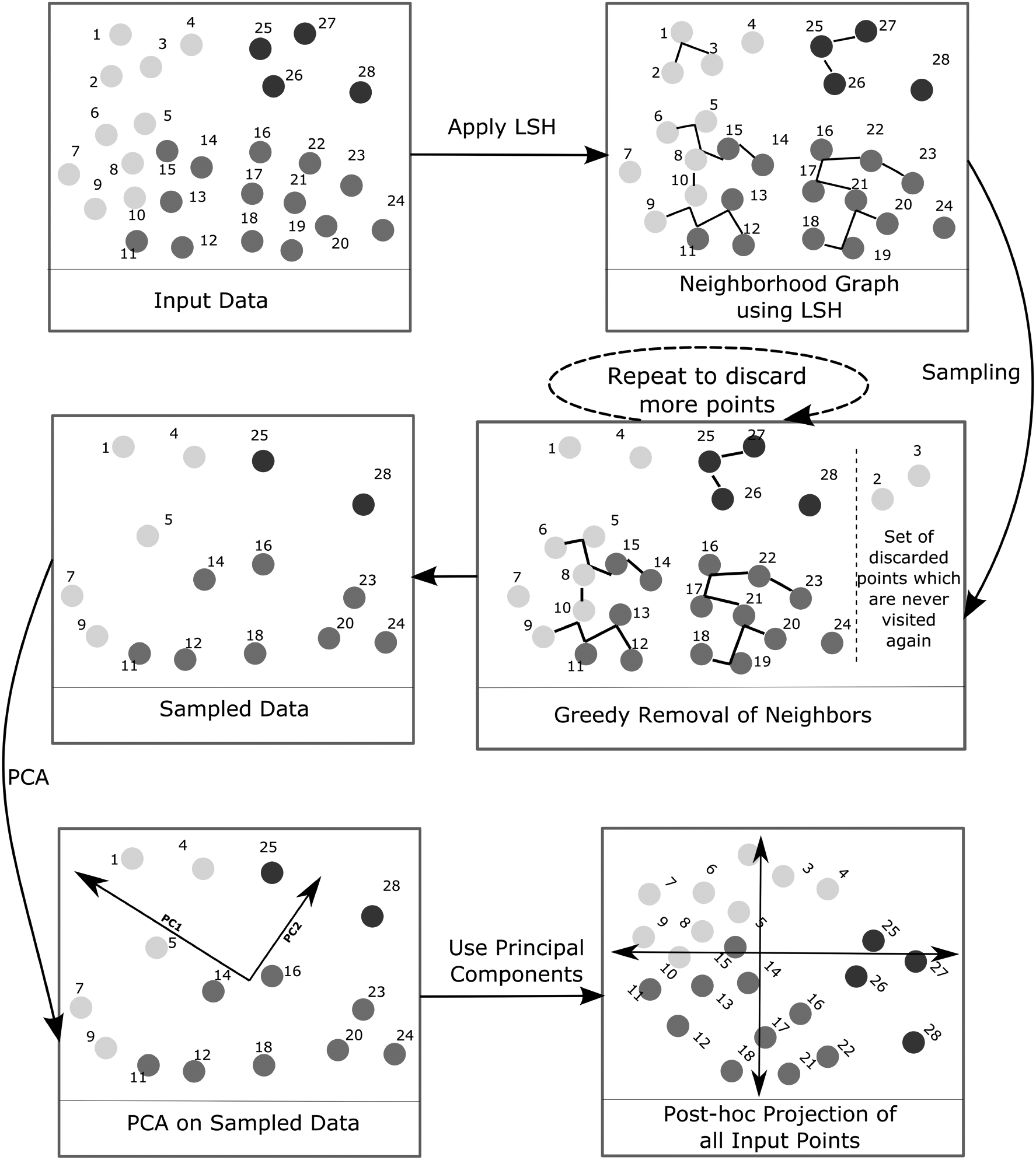
A pictorial view of the LSPCA algorithm. The solid circles represent individual samples of a data set. The numbers adjacent to each sample indicate the respective index. LSPCA, locality-sensitive principal component analysis.

4.1. LSH-based sampling

Input: Preprocessed data matrix, \documentclass{aastex}\usepackage{amsbsy}\usepackage{amsfonts}\usepackage{amssymb}\usepackage{bm}\usepackage{mathrsfs}\usepackage{pifont}\usepackage{stmaryrd}\usepackage{textcomp}\usepackage{portland, xspace}\usepackage{amsmath, amsxtra}\usepackage{upgreek}\pagestyle{empty}\DeclareMathSizes{10}{9}{7}{6}\begin{document} $${ \bf{X}}$$ \end{document} , containing normalized counts of filtered cells and top dispersed genes.

LSHForest: In this step, the hash codes of the input data points are produced. Unique hash codes that depict local regions or neighborhood are then computed. The python sklearn implementation of LSHForest module is used. The LSHForest is applied on the preprocessed data set with n_estimators = 30 and rest of the parameters are set to their defaults.

K-NN graph: An approximate neighborhood graph is obtained from the LSH tables. It is followed by searching for the 5-nearest neighbors (K-NN) of each point. This involves computing the Euclidean distances between the query point and its candidate neighbors.

Sampling: Sampling is carried out in a “greedy” manner. Each data point is visited sequentially in the same order as it appears in the original data set. During each visit, its respective 5-NN are flagged and never visited again. In this way, a subset of samples is obtained. The residue is further downsampled by performing the visit step recursively. For example, in the 68K PBMC data set, after 5 such iterations, ∼2000 samples were retained.

4.2. Computing LSPCA rotation matrix

LSPCA uses the structure preserving samples, \documentclass{aastex}\usepackage{amsbsy}\usepackage{amsfonts}\usepackage{amssymb}\usepackage{bm}\usepackage{mathrsfs}\usepackage{pifont}\usepackage{stmaryrd}\usepackage{textcomp}\usepackage{portland, xspace}\usepackage{amsmath, amsxtra}\usepackage{upgreek}\pagestyle{empty}\DeclareMathSizes{10}{9}{7}{6}\begin{document} $${ \cal S}{ \cal S} \subset { \bf{X}}$$ \end{document} , obtained in the previous step to compute its eigenvector matrix by using a standard PCA implementation. Performing SVD on LSH-based samples produces a transformation matrix similar to a PCA rotation matrix.

4.3. Post hoc projection onto the PCA space

The obtained transformation matrix, \documentclass{aastex}\usepackage{amsbsy}\usepackage{amsfonts}\usepackage{amssymb}\usepackage{bm}\usepackage{mathrsfs}\usepackage{pifont}\usepackage{stmaryrd}\usepackage{textcomp}\usepackage{portland, xspace}\usepackage{amsmath, amsxtra}\usepackage{upgreek}\pagestyle{empty}\DeclareMathSizes{10}{9}{7}{6}\begin{document} $$\mathcal{M}$$ \end{document} , is used to project the entire data set onto the new projection bias. The features in projected data are referred to as LSPCA components. \documentclass{aastex}\usepackage{amsbsy}\usepackage{amsfonts}\usepackage{amssymb}\usepackage{bm}\usepackage{mathrsfs}\usepackage{pifont}\usepackage{stmaryrd}\usepackage{textcomp}\usepackage{portland, xspace}\usepackage{amsmath, amsxtra}\usepackage{upgreek}\pagestyle{empty}\DeclareMathSizes{10}{9}{7}{6}\begin{document} \begin{align*} { \rm{LSPCA \ Component \ Matrix}} = { \bf{X}} \times \mathcal{M}. \end{align*} \end{document}

5. Data Description

Two types of single-cell data sets were used for the evaluation. The unannotated recount single-cell data sets comprised nine data sets sourced from the recount2 project (Collado-Torres et al., 2017). The second type contained two data sets with annotations. The summary of the data sets is provided in Table 1.

Recount is a multiexperiment resource of analysis-ready RNA-seq gene, and exon count data sets, recount2, are the later version of the recount project. This online resource consists of RNA-seq gene and exon counts along with their corresponding coverage bigWig files for 2041 different studies. All unannotated data sets used in our experiments were downloaded from (https://jhubiostatistics.shinyapps.io/recount).

Table 1.

Summary of the Data Sets Used in the Experiments

Serial No.	Data set name	Domain	Features	Instances
1	DRP001358	Human cancer cells	58037	337
2	DRP002435	Human HeLa cells	58037	477
3	GSE53529	Human myoblasts	58037	384
4	GSE57872	Human tumor cells	58037	875
5	GSE64016	Human embroyonic stem cells	58037	460
6	GSE66357	Human tonsil cells	58037	643
7	GSE67835	Human brain cells	58037	466
8	GSE70580	Human tonsil cells	58037	648
9	GSE75140	Human cerebral tissues	58037	734
10	PBMC	Fresh PBMC, healthy donor	32738	68793

PBMC, peripheral blood mononuclear cell.

One of these data sets, GSE67835, as also annotated and originated from profiling of 466 single cells isolated from the adult and fetal human brain tissues. The mixture contained populations of oligodendrocyte progenitors (OPC), oligodendrocytes, astrocytes, microglia, neurons, endothelial cells, replicating neuronal progenitors, and quiescent newly born neurons.

The PBMC data set prepared by Zheng et al. (2017) was downloaded from (https://support.10xgenomics.com/single-cell-gene-expression/data sets. The data are sequenced on Illumina NextSeq 500 high output with 20,000 reads per cell.

6. Results and Discussion

LSPCA was compared with (1) a standard PCA on whole data set and (2) PCA on a subset of data obtained through random sampling (RSPCA). The random sampling PCA uses random sampling instead of LSH-based sampling. The number of random samples was kept equal to the number of samples obtained from LSH-based sampling. We included this method to contrast the effectiveness of LSH-based sampling against random sampling. The PCA module from the python sklearn implementation was used for the standard PCA with svd_solver = “full.”

Every raw data set was processed as per the steps as outlined in Figure 1. The preprocessed data sets were then subjected to the three feature extraction variants: PCA, LSPCA, and RSPCA. For the clustering experiments, k-means was applied to the top 50 principal components obtained from the respective PCA variant. The best k for each of the unannotated data sets was determined using two strategies, namely Bayesian Information Criterion (Bhat and Kumar, 2010), and silhouette scores (Rousseeuw, 1987). The k corresponding to the highest score was chosen. Both the strategies reported the same value of k for each data set. In contrast, the k for the annotated data sets was set according to their respective known number of cell types.

6.1. Clustering accuracy

The clustering performance by respective PCA methods was reported using the silhouette score for the unannotated data sets and the ARI for the annotated data sets. In addition, the clustering accuracy of the minor cell type populations of the annotated data sets was examined exclusively.

6.1.1. Silhouette score

The silhouette score (or index) is an internal validity measure based on similarity of points within a cluster and separation across other clusters (Rousseeuw, 1987). It is used for validation of consistency within clusters of data when data labels are not present. A high average silhouette score indicates that the objects within a cluster are tightly placed and the individual clusters are well separated. Figure 3 shows the silhouette score for nine single-cell recount data sets clustered on the top 50 components obtained from the respective PCA variants. The comparative performance shows that the proposed LSPCA method gives a better lower dimensional representation of original data sets than the alternative variants of PCA.

FIG. 3.

Silhouette index of the unannotated data sets. The values adjacent to the bubble indicate the number of clusters for which the maximum silhouette score could be attained. The x-axis indicates the silhouette score.

6.1.2. Adjusted Rand index

Adjusted Rand Index (ARI) metric is a suitable choice to validate obtained clusters when the data is annotated. The PBMC and the Human Brain Cell data sets were used to demonstrate the concordance of the obtained clusters with the biological annotations. While all the ∼68K PBMC cells were annotated, it must be noted that in the Human Brain Cell data set (GSE67835), the annotations of neurons and OPCs cell types were found to be ambiguous, Darmanis et al. (2015), and were therefore removed from our cluster validation analysis. With this restriction, 268 out of 466 human brain cells were retained featuring astrocytes, endothelial, fetal-quiescent, fetal-replicating, microglia and oligodendrocyte cells.

The value of ARI is close to 0 when the clustering prediction is random, whereas the ARI is 1 when the clustering is perfectly identical to the true labels (Yeung and Ruzzo, 2001). Figure 4 shows the clustering performance on the PBMC and Human Brain Cell data sets for the different PCA methods. It is observed that the ARI scores obtained from PCA with LSH-based sampling are higher than traditional PCA or PCA with random sampling.

FIG. 4.

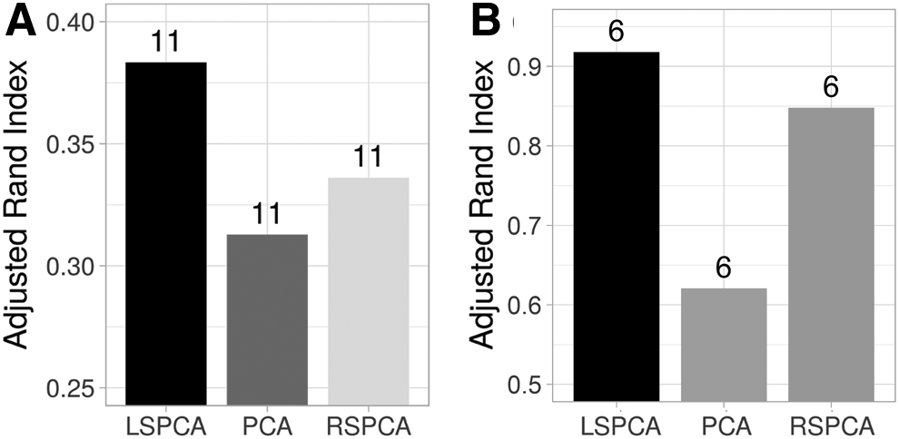
Comparing the k-means clustering accuracy evaluated using ARI of three PCA variants on (A) PBMC data set and (B) Human Brain tissue data set. The number of clusters, k, was set to the number of known cell types of the corresponding data set. ARI, adjusted Rand index; PBMC, peripheral blood mononuclear cell.

6.1.3. Discovery of small clusters

The effectiveness of sampling is more pronounced when the performance of clustering is measured only for the minority groups. For this measurement, we selected only those transcriptomes that shared the annotated groups of size ≤5% in the entire data set. Figure 5A shows the ARI computed for the transcriptomes appearing in minor groups of the ∼68K PBMC data set for all the methods. For all the categories, more accurate predictions were made when LSPCA was used.

FIG. 5.

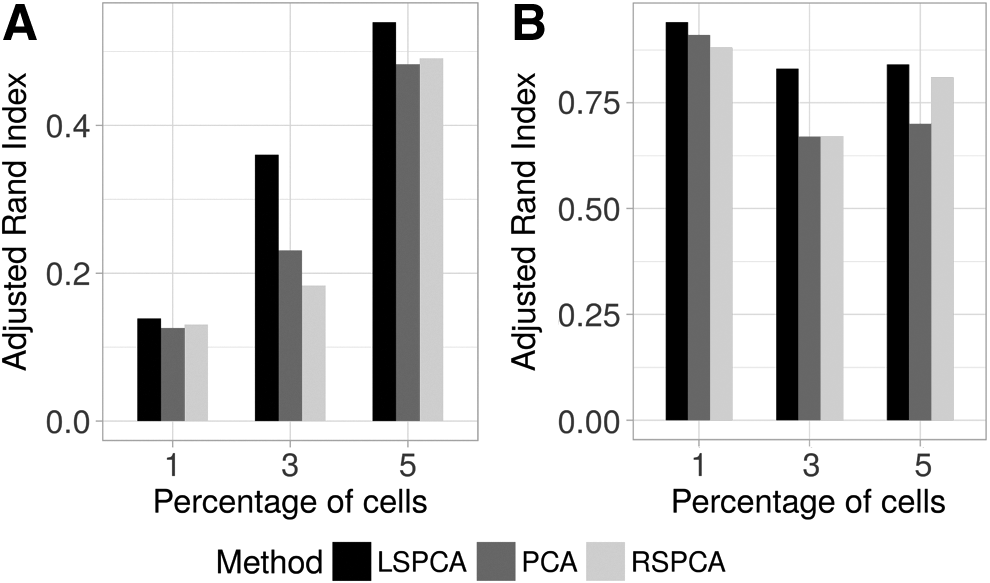
ARI to compare discordance of the predicted clusters discovered by the respective PCA variants with reference to the known annotations. (A) PBMC data set: members from the CD34⁺ (262 cells) and the CD4⁺ T Helper2 (19 cells) groups together constitute the 1% category. The 3% category contains the dendritic cells (1865 cells) in addition to the cells under the 1% category. The third subset includes the CD4⁺/CD45RA⁺/CD25⁻ Naive T (2793 cells) and the CD4⁺/CD45RO⁺ Memory (3126 cells); (B) Human Brain data set: Clustering performance compared on three data subsets containing a mixture of six different brain cell types with a concentration of oligodendrocytes at 1%, 3% and 5% corresponding to each subset.

For the Human Brain data set (GSE67835), minor cell types were simulated by gradually reducing the number of cells for one selected cell type. To this end, three different data subsets were derived by varying the concentration of oligodendrocytes at 5% (5 out of 244 cells), 3% (8 out of 239 cells) and 1% (3 out of 234 cells) respectively. As expected, in all the cases LSPCA maximized the ARI scores (Figure 5B).

6.2. Correlation with conventional principal components

This experiment measures the linear association between the first five principal components of LSPCA with the respective components obtained using the traditional PCA. The linear association was measured using Pearson's correlation coefficient. All the data sets were preprocessed before any PCA as shown in Figure 1. The RSPCA was also used to compare the effect of sampling. The correlation between the components of both the methods versus the respective first five components of standard PCA was recorded as shown in Figure 6. It is observed that the top LSPCA components correlate more with the traditional PCA than RSPCA for all the data sets.

FIG. 6.

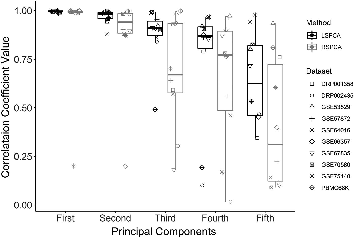
The box-plots show the distribution of Pearson's correlation coefficients between the respective components of a traditional PCA and LSPCA (dark) or RSPCA (light) across all the data sets. RSPCA, random sampling PCA.

6.3. Execution time

PCA took ∼1 hour on the PBMC data set compared with only ∼11 minutes by LSPCA. All experiments were carried out on a PC having an Intel Core i7-3770 3.40 GHz processor and 32 GB of RAM.

7. Conclusion

Overall, LSPCA is applicable wherever PCA is used, more specifically useful for large data sets like single-cell expression matrix. It is fast and produces components almost identical to the vanilla PCA components. The method provides flexibility to a user to adjust the number of samples to train the PCA with. It must be noted that LSPCA is not a new dimension reduction method, but when the data set is large, it assists PCA to work on a smaller subset whose members adequately represent the whole data set. Compared with random sampling, structure-aware sampling is a more effective way to sample from a large data set. LSPCA performs dimension reduction by operating on a subset of less redundant samples without significantly altering the performance of the classic PCA.

Software Availability

https://github.com/Snehalikalall/Lspca

Footnotes

Author Disclosure Statement

The authors declare that no competing financial interests exist.

References

Bawa

, Condie

, and Ganesan

2005. LSH Forest: Self-tuning indexes for similarity search, 651–660. In Proceedings of the 14th International Conference on World Wide Web. ACM, New York, NY.

Bhat

H.S.

, and Kumar

2010. On the Derivation of the Bayesian Information Criterion. School of Natural Sciences, University of California, California.

Chawla

N.V.

, Bowyer

K.W.

, Hall

L.O.

, et al. 2002. Smote: Synthetic minority over-sampling technique. J. Artif. Intell. Res. 16, 321–357.

Collado-Torres

, Nellore

, Kammers

, et al. 2017. Reproducible RNA-seq analysis using recount2. Nat. Biotechnol., 35, 319–321.

Darmanis

, Sloan

S.A.

, and Zhang

, et al. 2015. A survey of human brain transcriptome diversity at the single cell level. Proceedings of the National Academy of Science, 112, 7285–7290.

Grün

, Lyubimova

, Kester

, et al. 2015. Single-cell messenger RNA sequencing reveals rare intestinal cell types. Nature, 525, 251–255.

Indyk

, Motwani

, Raghavan

, et al. 1997. Locality-preserving hashing in multidimensional spaces, 618–625. In Proceedings of the Twenty-ninth Annual ACM Symposium on Theory of Computing. ACM, New York, NY.

Jolliffe

I.T.

1986. Principal component analysis and factor analysis, 115–128. In Principal Component Analysis. Springer, New York, NY.

Karamizadeh

, Abdullah

S.M.

, Manaf

A.A.

, et al. 2013. An overview of principal component analysis. J. Signal Inf. Process. 4, 173.

10.

Leskovec

, Rajaraman

, and Ullman

J.D.

2014. Mining of Massive Datasets. Cambridge University Press, Cambridge, UK.

11.

, Diao

, Ma

, et al. 2008. A statistical PCA method for face recognition, 376–380. In Second International Symposium on Intelligent Information Technology Application, 2008. IITA’08, volume 3. IEEE, Los Alamitos, CA.

12.

Macosko

E.Z.

, Basu

, Satija

, et al. 2015. Highly parallel genome-wide expression profiling of individual cells using nanoliter droplets. Cell, 161, 1202–1214.

13.

Martinsson

P.-G.

, Rokhlin

, and Tygert

2011. A randomized algorithm for the decomposition of matrices. Appl. Comput. Harmon. Anal. 30, 47–68.

14.

Pauleve

, Jegou

, and Amsaleg

2010. Locality sensitive hashing: A comparison of hash function types and querying mechanisms. Pattern Recognit. Lett. 31, 1348–1358.

15.

Rousseeuw

P.J.

1987. Silhouettes: A graphical aid to the interpretation and validation of cluster analysis. J. Comput. Appl. Math. 20, 53–65.

16.

Shalek

A.K.

, Satija

, Adiconis

, et al. 2013. Single-cell transcriptomics reveals bimodality in expression and splicing in immune cells. Nature, 498, 236–240.

17.

Wagner

, Regev

, and Yosef

2016. Revealing the vectors of cellular identity with single-cell genomics. Nat. Biotechnol., 34, 1145–1160.

18.

Yeung

K.Y.

, and Ruzzo

W.L.

2001. Details of the adjusted Rand index and clustering algorithms, supplement to the paper “An empirical study on Principal Component Analysis for clustering gene expression data.”. Bioinformatics, 17, 763–774.

19.

Zheng

G.X.

, Terry

J.M.

, Belgrader

, et al. 2017. Massively parallel digital transcriptional profiling of single cells. Nat. Commun. 8, 14049.