Human Splice-Site Prediction with Deep Neural Networks

Abstract

Accurate splice-site prediction is essential to delineate gene structures from sequence data. Several computational techniques have been applied to create a system to predict canonical splice sites. For classification tasks, deep neural networks (DNNs) have achieved record-breaking results and often outperformed other supervised learning techniques. In this study, a new method of splice-site prediction using DNNs was proposed. The proposed system receives an input sequence data and returns an answer as to whether it is splice site. The length of input is 140 nucleotides, with the consensus sequence (i.e., “GT” and “AG” for the donor and acceptor sites, respectively) in the middle. Each input sequence model is applied to the pretrained DNN model that determines the probability that an input is a splice site. The model consists of convolutional layers and bidirectional long short-term memory network layers. The pretraining and validation were conducted using the data set tested in previously reported methods. The performance evaluation results showed that the proposed method can outperform the previous methods. In addition, the pattern learned by the DNNs was visualized as position frequency matrices (PFMs). Some of PFMs were very similar to the consensus sequence. The trained DNN model and the brief source code for the prediction system are uploaded. Further improvement will be achieved following the further development of DNNs.

1. Introduction

Accurate splice-site prediction from genome sequence data is essential to delineate gene structures and alternative splice variants. However, splice sites revealed by alignment are not always reliable, because the chance of randomly mapping a short read to a large reference genome is high. Therefore, computational methods are helpful for splice-site prediction.

For computational prediction, it is necessary to know the pattern of the sequences of splice sites, which are regions where introns are excised from the pre-mRNA, while leaving the exons intact. In general, the exon/intron boundary is called the donor (5′) splice site, whereas the intron/exon boundary is called the acceptor (3′) splice site and is conserved with the dinucleotide AG, known as the canonical splice site. Although several eukaryotic organisms contain two kinds of spliceosomes, that is, the U2-type and U12-type, the vast majority of introns are the U2-type. Most of the donor sites in U2-type introns contain the GT dinucleotide at the intron boundary, whereas the GC dinucleotide is observed in <1% of cases (Sheth et al., 2006). This donor site is recognized by the U1 snRNA of the spliceosome through base-pairing with an ACUUACCU motif; nevertheless, the donor-site pattern is not uniform and tolerates several variations in the motif, except for the GT dinucleotide at the boundary. The acceptor site almost always contains the AG dinucleotide at the intron boundary, with an even less explicit pattern around the AG dinucleotide. As such, all GT (AG) dinucleotides within the DNA molecule are defined as candidate donor (acceptor) sites and are judged as either a true or a false site.

To accurately predict splice sites, different computational algorithms have been developed, including Bayesian networks (Chen et al., 2005), support vector machine (SVM) (Degroeve et al., 2005; Baten et al., 2006; Sonnenburg et al., 2007; Wei et al., 2013; Meher et al., 2016), hidden Markov model (Pertea et al., 2001; Stanke and Waack, 2003; Zhang et al., 2010; Pashaei et al., 2016), and random forests (Pashaei et al., 2016).

Deep neural networks (DNNs) have achieved record-breaking results, primarily due to the recent revival of deep convolutional neural networks (CNNs) for processing of images (Krizhevsky et al., 2012), video, speech, and audio on highly challenging data sets using purely supervised learning. There are several successful examples of the application of DNNs to detect genomic problems. DeepSEA is used to predict chromatin effects of sequence alterations and prioritize functional single-nucleotide polymorphisms by learning a regulatory sequence code from large-scale chromatin-profiling data (Zhou and Troyanskaya, 2015). Improved performance for this task was reported using DanQ (Quang and Xie, 2016), a hybrid DNN (Graves, 2005). DeepSplice is a novel tool for splice-site prediction based on deep CNNs (Zhang et al., 2016) that differs from other methods for splice-site prediction, because predictions are made by combining the information of the donor and acceptor sites instead of each individual site. However, no DNN system for individual splice-site prediction has yet been developed; therefore, it is unknown whether such a system can achieve remarkable performance. In this study, we presented a new system for individual splice-site prediction based on DNN. The generated data set was tested with some previous methods.

2. Methods

2.1. Data set

The Homo Sapiens Splice-Site Data set HS3D, downloaded from www.sci.unisannio.it/docenti/rampone, was used to create a prediction model and test the performance of the proposed system. This data set has been used in previous methods (Zhang et al., 2010; Wei et al., 2013; Meher et al., 2016; Pashaei et al., 2016); therefore, comparisons with previous studies are relatively simple. The data set contains 2796 true donor sites, 2880 true acceptor sites, 271,937 false donor sites, and 329,374 false acceptor sites. The length of both the true and false splice-site sequences is 140 nucleotides, with the consensus nucleotides GT at positions 71 and 72 for donor sites and the consensus nucleotides AC at positions 69 and 70 for acceptor splice sites.

First, all true splice sites were selected and we randomly selected the same number of false sites. In this case, the ratio between the number of true and false splice sites was 1:1. Second, a 1:10 data set was constructed, which contained all true splice sites, and we randomly selected false splice sites with numbers 10 times greater than that for true splice sites.

2.2. DNN architecture

Each input layer consisted of sequence data encoded as one hot vector, where each position consists of a five-element vector with one nucleotide bit set to one. Two convolutional layers follow the input layer, with max-pooling layers. A hybrid model combining CNN and bidirectional long short-term memory network (BLSTM) was shown to outperform the CNN model in predicting the function of noncoding DNA (Quang and Xie, 2016); therefore, the proposed hybrid model was tested. In this study, the model without the BLSTM layer was referred to as the CNN model and that with the BLSTM layer as the hybrid model. The CNN model was compared with the hybrid model. The last two layers were fully connected and the binary output layer with SoftMax activation returned the probability of a splice site. Dropout (Srivastava et al., 2014) was used on the convolutional, BLSTM, and fully connected layers.

The Adam (Kingma and Ba, 2014) optimizer was used for training with categorical cross-entropy as a loss of function. The number of convolutional layers was set to two. Balancing between discovering more complex relationships was associated with a risk of overfitting (Karsoliya, 2012). Other hyperparameters such as the number of filters and the window sizes of the convolutional and BLSTM layers were determined based on a random search in consideration of the training and processing time (Bergstra and Bengio, 2012). The proposed model, as shown in Figure 1, was implemented using Keras (https://github.com/fchollet/keras), which is a highly modular DNN library written in Python.

FIG. 1.

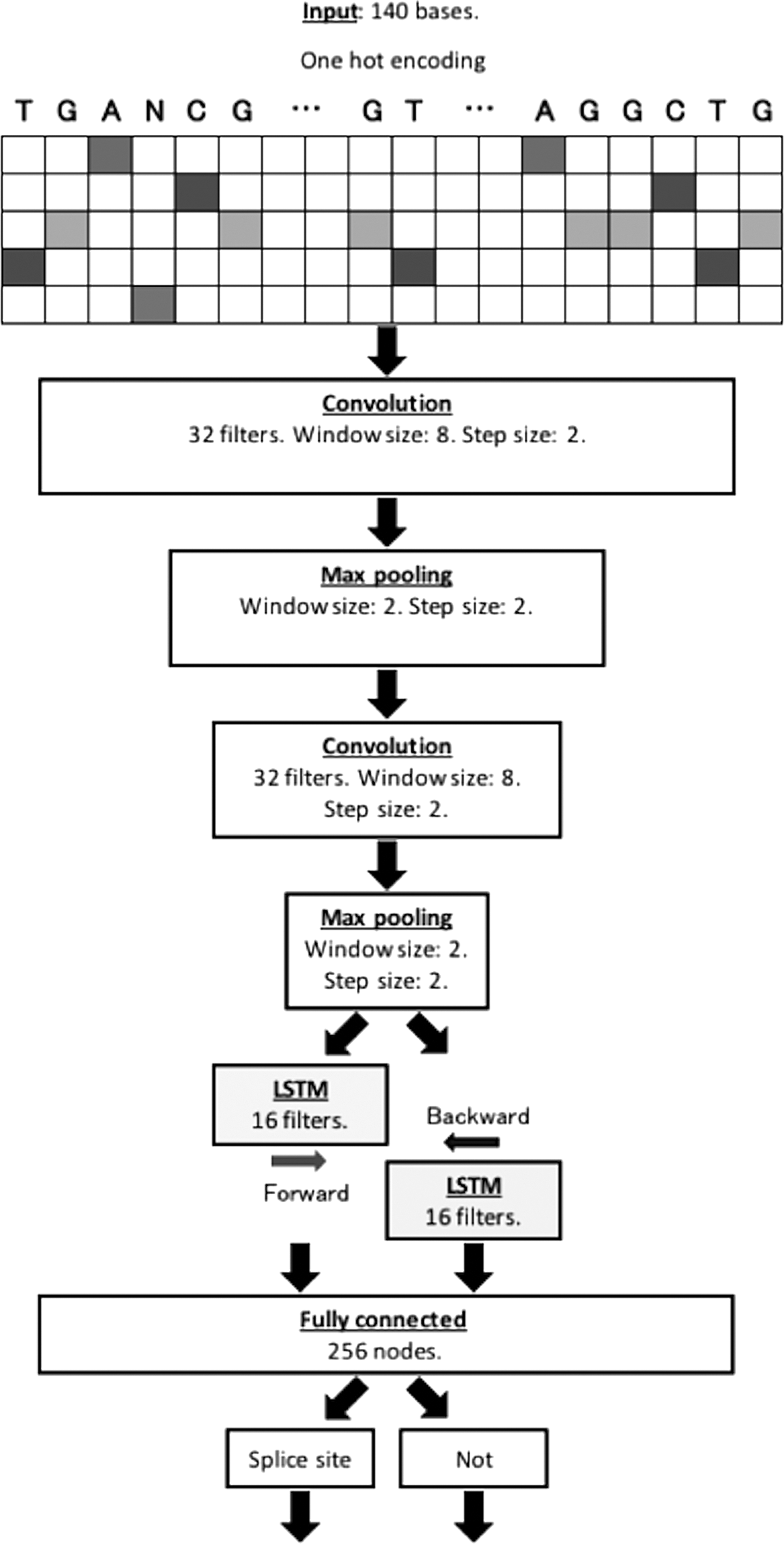
A graphical illustration of the proposed model. An input sequence is encoded to one hot vector of a five-row bit matrix. Two convolutional layers follow with max-pooling layers. Only in the hybrid model, additional BLSTM layers follow. Dropout layers followed the convolutional and BLSTM layers during the training periods. After a fully connected layer, the probability of a splice site is determined. BLSTM, bidirectional long short-term memory network; LSTM, long short-term memory network.

2.3. Estimated parameters for performance evaluation

The performance evaluation of the proposed method was performed with a 10-fold cross-validation of the data set. Then, the average performance estimation was calculated. This process was repeated five times and the final average with the 95% confidence interval was reported. Estimated parameters include sensitivity (Sn), specificity (Sp), global accuracy (Q⁹) (Zhang and Zhang, 2002), and the Matthews correlation coefficient (Mcc), which were defined as \documentclass{aastex}\usepackage{amsbsy}\usepackage{amsfonts}\usepackage{amssymb}\usepackage{bm}\usepackage{mathrsfs}\usepackage{pifont}\usepackage{stmaryrd}\usepackage{textcomp}\usepackage{portland, xspace}\usepackage{amsmath, amsxtra}\usepackage{upgreek}\pagestyle{empty}\DeclareMathSizes{10}{9}{7}{6}\begin{document} \begin{align*} Sn = { \frac { TP } { TP + FN } } \end{align*} \end{document} \documentclass{aastex}\usepackage{amsbsy}\usepackage{amsfonts}\usepackage{amssymb}\usepackage{bm}\usepackage{mathrsfs}\usepackage{pifont}\usepackage{stmaryrd}\usepackage{textcomp}\usepackage{portland, xspace}\usepackage{amsmath, amsxtra}\usepackage{upgreek}\pagestyle{empty}\DeclareMathSizes{10}{9}{7}{6}\begin{document} \begin{align*} Sp = { \frac { TP } { TP + FP } } \end{align*} \end{document} \documentclass{aastex}\usepackage{amsbsy}\usepackage{amsfonts}\usepackage{amssymb}\usepackage{bm}\usepackage{mathrsfs}\usepackage{pifont}\usepackage{stmaryrd}\usepackage{textcomp}\usepackage{portland, xspace}\usepackage{amsmath, amsxtra}\usepackage{upgreek}\pagestyle{empty}\DeclareMathSizes{10}{9}{7}{6}\begin{document} \begin{align*} \ \ {Q^9} = \left( {1 + {q^9}} \right) / 2 \end{align*} \end{document}

where \documentclass{aastex}\usepackage{amsbsy}\usepackage{amsfonts}\usepackage{amssymb}\usepackage{bm}\usepackage{mathrsfs}\usepackage{pifont}\usepackage{stmaryrd}\usepackage{textcomp}\usepackage{portland, xspace}\usepackage{amsmath, amsxtra}\usepackage{upgreek}\pagestyle{empty}\DeclareMathSizes{10}{9}{7}{6}\begin{document} \begin{align*} {q^2} = \left\{ { \begin{matrix} {{{TN - FP} \over {TN + FP}} \ if \ TP + FN = 0} \\ {{{TP - FN} \over {TP + FN}} \ if \ TN + FP = 0} \\ {1 - \root {} \of {2 \left[ {{{ \left( {{{FN} \over {TP + FN}}} \right) }^2} + {{ \left( {{{FP} \over {TN + FP}}} \right) }^2}} \right] } \ if \ TP + FN \, \ne 0 \ and \ TN + FP \, \ne 0} \\ \end{matrix} } \right. \end{align*} \end{document} \documentclass{aastex}\usepackage{amsbsy}\usepackage{amsfonts}\usepackage{amssymb}\usepackage{bm}\usepackage{mathrsfs}\usepackage{pifont}\usepackage{stmaryrd}\usepackage{textcomp}\usepackage{portland, xspace}\usepackage{amsmath, amsxtra}\usepackage{upgreek}\pagestyle{empty}\DeclareMathSizes{10}{9}{7}{6}\begin{document} \begin{align*} Mcc = { \frac { TP*TN - FP*FN } { \root { } \of { \left( { TP + FN } \right) * \left( { TN + FP } \right) * \left( { TP + FP } \right) * \left( { TN + FN } \right) } } } \end{align*} \end{document}

where TP, TN, FP, and FN are the numbers of true positives, true negatives, false positives, and false negatives, respectively.

In addition, the area under the receiver operating characteristic curve (ROC-AUC) was calculated for comparisons between models with and without a BLSTM layer.

2.4. Visualization of what the proposed model learned

The pattern learned by the proposed model was visualized as position frequency matrices (PFMs), which were generated using a similar approach described by DeepBind (Alipanahi et al., 2015). The convolutional filters of the hybrid model with the highest ROC-AUC learned from the 1:1 data set were used for visualization.

Let S = {s₁, …, s_i, …, s₁₄₀} be an input sequence and Y_{k, i} be the output value of k_th (1 ≤ k ≤ 32) convolutional filter for some position i (1 ≤ i ≤ 133). For filter k, we only consider sequence s if Y_k,i > 0 for some position i. We find the position j = argmax i Y_k,i, and extract subsequence s_j–m₊₁… of length m, where m is the length of the motifs (i.e., the length of convolutional filters) in the proposed model. When \documentclass{aastex}\usepackage{amsbsy}\usepackage{amsfonts}\usepackage{amssymb}\usepackage{bm}\usepackage{mathrsfs}\usepackage{pifont}\usepackage{stmaryrd}\usepackage{textcomp}\usepackage{portland, xspace}\usepackage{amsmath, amsxtra}\usepackage{upgreek}\pagestyle{empty}\DeclareMathSizes{10}{9}{7}{6}\begin{document} $$\forall {Y_k} \leq 0$$ \end{document} , filter k is skipped. Once extracted, all subsequences are stacked and the base frequencies are counted to generate a PFM of length m.

3. Results and Discussion

3.1. Comparison between the hybrid and convolutional neural network models

Figure 2 shows the comparison of ROC-AUCs between the CNN and hybrid models. At the donor site, ROC-AUC of the hybrid models was higher than that of the CNN models for 66% of units of the 1:1 data set and for 76% of units of the 1:10 data set. At the acceptor site, ROC-AUC of the hybrid models was higher than that of the CNN models for 66% of units of the 1:1 data set and 68% of units of the 1:10 data set. Table 1 shows the Sn, Sp, Q⁹, and Mcc values of the hybrid and CNN models. All estimated parameters of the hybrid model were higher than those of the CNN model for both the 1:1 and 1:10 data sets, although there were some differences in parameters between models. Therefore, the hybrid model, rather than the CNN model, was used in the following analyses. One possible explanation for these results is that additional BLSTM layers can improve the prediction ability. The current candidate sequences have consensus sequences in the middle, and it is assumed that the closer a base is to the middle, the more important it is for splice-site prediction. Therefore, additional BLSTM layers are helpful in that the forward LSTM can learn the successive sequence information from the 5′ end to the middle, whereas the backward LSTM can learn the information from the 3′ end to the middle.

FIG. 2.

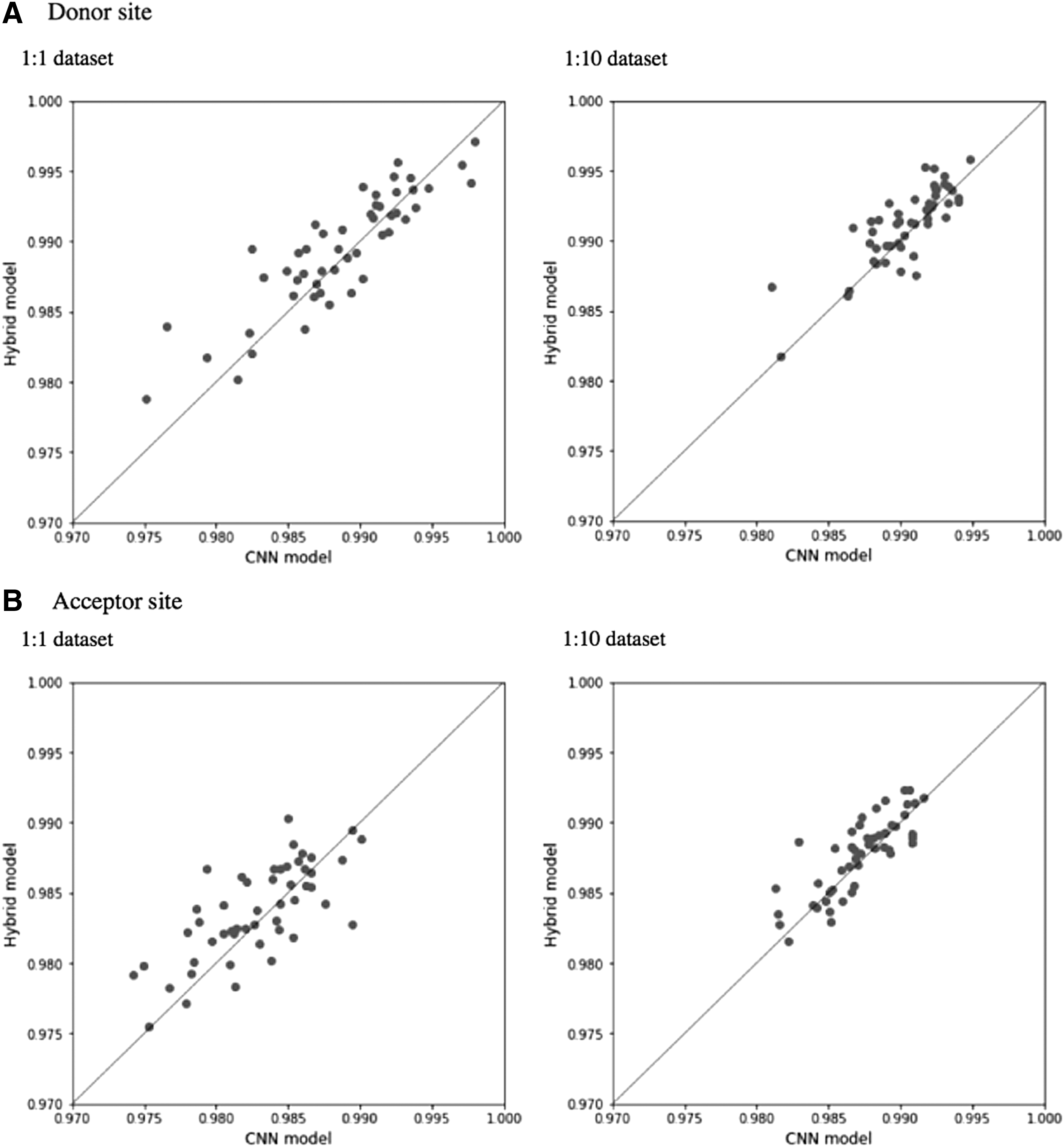
Scatter plots comparing ROC-AUCs of the CNN and hybrid models. Results for the donor site (A) and acceptor site (B). The left panels are scatter plots of the 1:1 data set, and the right panels are scatter plots of the 1:10 data set. The horizontal axes indicate ROC-AUC of the CNN model, and the vertical axes indicate ROC-AUC of the hybrid model. ROC-AUC of the hybrid model was higher than that of the CNN model for more than half of the units of all data sets. AUC, area under the curve; CNN, convolutional neural network; ROC, receiver operating characteristic.

Table 1.

Summary of Performance Evaluation of the Convolutional Neural Network and Hybrid Models

	Donor site				Acceptor site
Methods	Sn	Sp	Q9	Mcc	Sn	Sp	Q9	Mcc
1:1 data set
CNN	97.80 ± 0.3	95.06 ± 0.3	96.08 ± 0.2	92.91 ± 0.4	96.15 ± 0.3	93.24 ± 0.4	94.41 ± 0.2	89.45 ± 0.4
Hybrid	97.88 ± 0.3	95.36 ± 0.3	96.27 ± 0.2	93.33 ± 0.4	96.42 ± 0.4	93.34 ± 0.4	94.57 ± 0.2	89.87 ± 0.4
1:10 data set
CNN	89.61 ± 0.8	98.66 ± 0.1	92.58 ± 0.6	87.11 ± 0.4	84.40 ± 0.8	98.43 ± 0.1	88.91 ± 0.6	82.82 ± 0.5
Hybrid	90.31 ± 0.6	98.75 ± 0.1	93.08 ± 0.4	87.99 ± 0.4	84.41 ± 0.7	98.59 ± 0.1	88.93 ± 0.5	83.60 ± 0.4

3.2. Comparison between the proposed model and previous methods

Table 2 shows the performance comparison of the proposed model with previous methods, such as a first-order Markov model with SVM (MM1-SVM), reduced MM1-SVM, SVM with a Bayes kernel, and MM1 with random forest (MM1-RF) (Pashaei et al., 2016). It is remarkable that the proposed model outperformed the previous methods in all performance metrics both for the donor and acceptor sites in the 1:1 data set. In the 1:10 dataset, the Sp values of DNN were obviously higher, whereas the Sn values of DNN were lower than those of other methods for both splice sites. The Mcc and Q⁹ values of the proposed model were higher than those of all previous methods for the donor site, whereas the Q⁹ value of the proposed model was lower than some of the previous methods for the acceptor site. Adjustment of the probability cutoff value of the splice site can modify the balance between Sp and Sn values. When setting the cutoff value at 0.3, the Q⁹ and Mcc values of the proposed model were 91.98 ± 0.2 and 82.05 ± 0.2, respectively, which were higher than those of all previous methods. The evaluation of the cutoff value adjustment is shown in Figure 3.

FIG. 3.

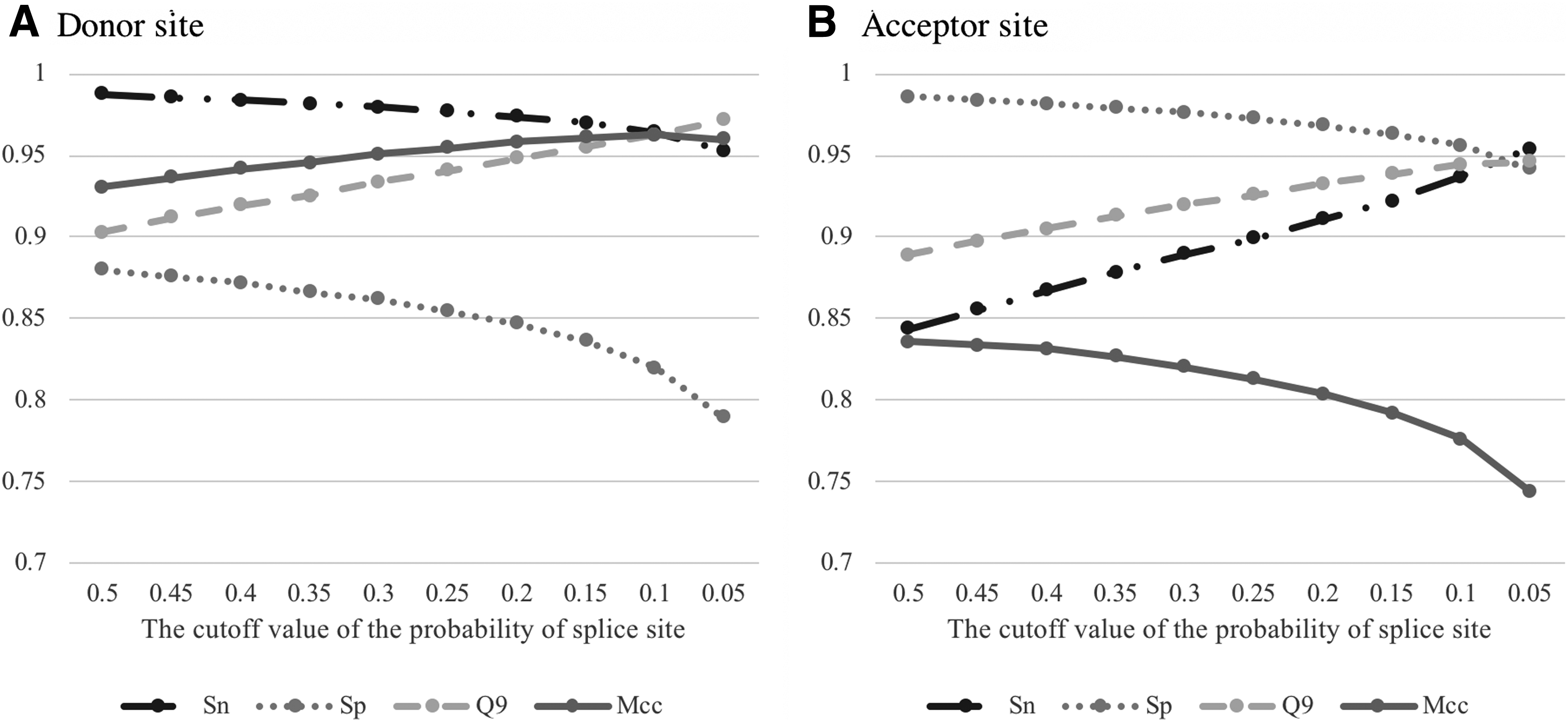
Adjustment of the cutoff value of probability that an input sequence is splice site. Results for the donor (A) and the acceptor (B) sites. The probability cutoff value was tested from 0.5 to 0.05 at intervals of 0.05. The mean Sp, Sq, Q9, and Mcc values of each cutoff are shown. For the acceptor site, when setting the cutoff value between 0.25 and 0.35, the values of both Q9 and Mcc were higher than those obtained by previous methods.

Table 2.

Summary of Performance Evaluations of the Proposed Deep Neural Network Model and Previous Methods

	Donor site				Acceptor site
Methods	Sn	Sp	Q9	Mcc	Sn	Sp	Q9	Mcc
1:1 data set
MM1-SVM	93.40 ± 0.1	91.20 ± 0.1	92.16 ± 0.1	84.64 ± 0.2	90.51 ± 0.1	86.89 ± 0.1	88.48 ± 0.1	77.48 ± 0.2
Reduced MM1-SVM	93.70 ± 0.0	91.51 ± 0.2	92.42 ± 0.1	85.26 ± 0.2	90.84 ± 0.1	87.12 ± 0.1	88.76 ± 0.1	78.03 ± 0.1
SVM-B	95.01 ± 0.1	90.26 ± 0.1	92.22 ± 0.0	85.37 ± 0.1	91.78 ± 0.1	87.21 ± 0.0	89.17 ± 0.0	79.10 ± 0.0
MM1-RF	95.46 ± 0.1	90.89 ± 0.2	92.74 ± 0.1	86.45 ± 0.3	91.77 ± 0.1	89.13 ± 0.1	90.27 ± 0.0	80.95 ± 0.1
DNN (hybrid)	97.88 ± 0.3	95.36 ± 0.3	96.27 ± 0.2	93.33 ± 0.4	96.42 ± 0.4	93.34 ± 0.4	94.57 ± 0.2	89.87 ± 0.4
1:10 data set
MM1-SVM	93.09 ± 0.3	91.32 ± 0.5	92.08 ± 0.3	84.64 ± 0.2	91.12 ± 0.1	87.47 ± 1.0	89.07 ± 0.6	77.48 ± 0.2
Reduced MM1-SVM	93.79 ± 0.2	91.24 ± 0.5	92.34 ± 0.3	85.26 ± 0.2	90.95 ± 0.1	88.38 ± 0.2	89.51 ± 0.1	78.03 ± 0.1
SVM-B	94.77 ± 0.2	90.92 ± 0.5	92.50 ± 0.2	85.37 ± 0.1	92.47 ± 0.0	87.62 ± 0.7	89.70 ± 0.4	79.10 ± 0.0
MM1-RF	95.09 ± 0.0	91.52 ± 0.2	93.01 ± 0.1	86.45 ± 0.3	91.96 ± 0.1	89.53 ± 0.5	90.58 ± 0.3	80.95 ± 0.1
DNN	90.31 ± 0.6	98.75 ± 0.1	93.08 ± 0.4	87.99 ± 0.4	84.41 ± 0.7	98.59 ± 0.1	88.93 ± 0.5	83.60 ± 0.4

DNN, deep neural network; MM1-SVM; first-order Markov model with support vector machine.

3.3. Visualization of what the proposed model learned

In PFMs generated from the first 32 convolutional filters, the PFM that is most similar to the PFM of the consensus motif of the canonical donor splice site (Burset et al., 2000) is shown in Figure 4. The PFM that is the most similar to the consensus motif of canonical acceptor site was determined in the same manner. The consensus motif and PFM generated from the model were very similar, thus visualization of the convolutional filters may have the potential to detect unknown motifs.

FIG. 4.

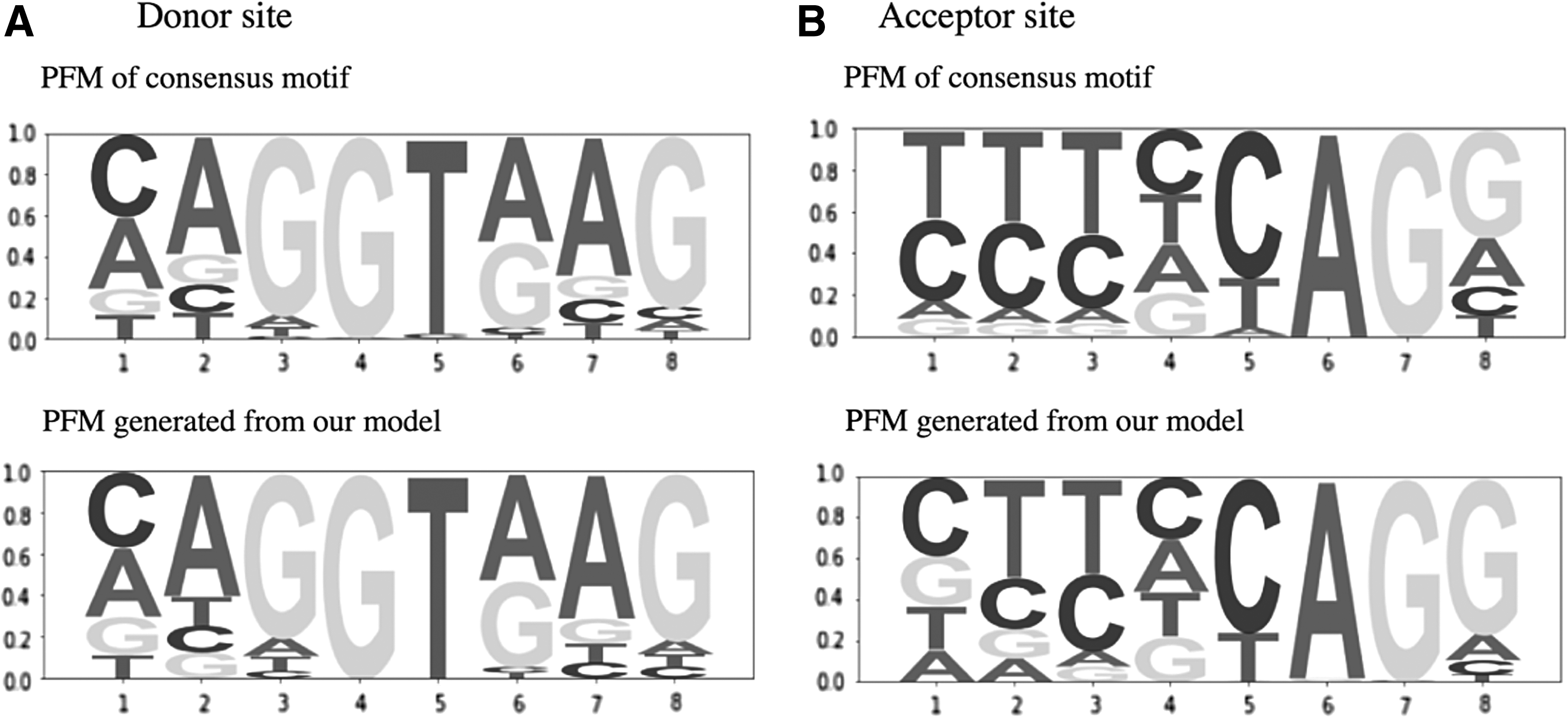
The consensus motifs and the motifs generated from the first convolutional layers. PFMs of the donor (A) and the acceptor (B) sites. PFM of the consensus motif and that generated from the proposed model are shown in the upper and lower figures, respectively. PFM, position frequency matrix.

4. Conclusions

In conclusion, a system to predict a splice site from the information of sequence data alone was developed using DNNs. The performance evaluation results showed that the proposed model outperformed previous methods using the same data set. In addition, combining CNNs and BLSTMs may improve prediction performance. There is an extremely active community researching deep learning; therefore, we believe that current and future insights will lead to greater performance for this task.

5. Availability

The source code and the trained models were uploaded as Deep Splice Site Prediction system (“DSSP”) to the GitHub repository (https://github.com/DSSP-github/DSSP) to facilitate the use of our classifiers and the development of similar tools. The sequence data used in training the model consisted of 140 bases; however, the system can be used for shorter sequences by complementing missing bases as “N.”

Footnotes

Author Disclosure Statement

No competing financial interests exist.

References

Baten

, Chang

, Halgamuge

, et al. 2006. Splice site identification using probabilistic parameters and SVM classification. BMC Bioinformatics. 7, S15.

Bergstra

, and Bengio

2012. Random search for hyper-parameter optimization. J. Mach. Learn. Res., 13, 281–305.

Burset

, Seledtsov

I.A.

, and Solovyev

V.V.

2000. Analysis of canonical and non-canonical splice sites in mammalian genomes. Nucleic Acids Res. 28, 4364–4375.

Chen

T.M.

, Lu

C.C.

, and Li

W.H.

2005. Prediction of splice sites with dependency graphs and their expanded bayesian networks. Bioinformatics, 21, 471–482.

Degroeve

, Saeys

, De Baets

, et al. 2005. SpliceMachine: Predicting splice sites from high-dimensional local context representations. Bioinformatics, 21, 1332–1338.

Graves

2005. Framewise phoneme classification with bidirectional LSTM and other neural network architectures. Neural Netw. 18, 602–610.

Karsoliya

2012. Approximating number of hidden layer neurons in multiple hidden layer BPNN architecture. Int. J. Eng. Trends Technol., 3, 714–717.

Kingma

, and Ba

2014. Adam: A method for stochastic optimization. arXiv:1412.6980 [cs.LG] 1–15.

Krizhevsky

, Sutskever

, and Hinton

G.E.

2012. ImageNet classification with deep convolutional neural networks. NIPS Proc. 1, 1097–1105.

10.

Meher

P.K.

, Sahu

T.K.

, Rao

A.R.

, et al. 2016. Identification of donor splice sites using support vector machine: A computational approach based on positional, compositional and dependency features. Algorithms Mol. Biol. 11, 1–12.

11.

Pashaei

, Ozen

, and Aydin

2016. Random Forest in Splice Site Prediction of Human Genome. IFMBE Proc. 57, 518–523.

12.

Pertea

, Lin

, and Salzberg

S.L.

2001. GeneSplicer: A new computational method for splice site prediction. Nucleic Acids Res. 29, 1185–1190.

13.

Quang

, and Xie

2016. DanQ: A hybrid convolutional and recurrent deep neural network for quantifying the function of DNA sequences. Nucleic Acids Res. 44, 1–6.

14.

Sheth

, Roca

, Hastings

M.L.

, et al. 2006. Comprehensive splice-site analysis using comparative genomics. Nucleic Acids Res. 34, 3955–3967.

15.

Sonnenburg

, Schweikert

, Philips

, et al. 2007. Accurate splice site prediction using support vector machines. BMC Bioinformatics. 8, S7.

16.

Srivastava

, Hinton

G.E.

, Krizhevsky

, et al. 2014. Dropout: A simple way to prevent neural networks from overfitting. J. Mach. Learn. Res. 15, 1929–1958.

17.

Stanke

, and Waack

2003. Gene prediction with a hidden Markov model and a new intron submodel. Bioinformatics, 19, 215–225.

18.

Wei

, Zhang

, Wei

, et al. 2013. A novel splice site prediction method using support vector machine. J. Comput. Inf. Syst., 20, 8053–8060.

19.

Zhang

C.T.

, and Zhang

2002. Evaluation of gene-finding algorithms by a content-balancing accuracy index. J. Biomol. Struct. Dyn., 19, 1045–1052.

20.

Zhang

, Peng

, Zhang

, et al. 2010. Splice sites prediction of Human genome using length-variable Markov model and feature selection. Expert Syst. Appl., 37, 2771–2782.

21.

Zhang

, Liu

, Macleod

J.N.

, et al. 2016. DeepSplice: Deep classification of novel splice junctions revealed by RNA-seq, 330–333. Presented at the 2016 IEEE International Conference on Bioinformatics and Biomedicine.

22.

Zhou

, and Troyanskaya

O.G.

2015. Predicting effects of noncoding variants with deep learning-based sequence model. Nat. Methods., 12, 931–934.