More and more evidence shows that microbes play crucial roles in human health and disease. The exploration of the relationship between microbes and diseases will help people to better understand the underlying pathogenesis and have important implications for disease diagnosis and prevention. However, the known associations between microbes and diseases are very less. We proposed a new method called non-negative matrix factorization microbe–disease associations (NMFMDA), which used Gaussian interaction profile kernel similarity measure, to calculate microbial similarity and disease similarity, and applied a logistic function to regulate disease similarity. And, based on the known microbe–disease associations, a graph-regularized non-negative matrix factorization model was utilized to simultaneously identify potential microbe–disease associations. Moreover, fivefold cross-validation was utilized to evaluate the performance of our method. It reached the reliable area under receiver operating characteristic curve (AUC) of 0.8891, higher than other state-of-the-art methods. Finally, the case studies on three complex human diseases (i.e., asthma, inflammatory bowel disease, and colon cancer) demonstrated the good performance of our method. In summary, our method can be considered as an effective computational model for predicting potential disease–microbe associations.
1. Introduction
Microbes are small individuals such as bacteria, viruses, and some small primitive organisms, closely related to humans. There are many kinds of cells in and on the human body, ∼90% of them are microbial cells (Althani et al., 2016). These microbes live in the body's mouth, skin, vagina, and lungs, and most of them live in the gastrointestinal tract (Holmes et al., 2015). These microbes maintain a certain balance in the human body to help enhance immunity, promote metabolism, and regulate the gastrointestinal tract to keep human health (Ventura et al., 2009). For example, in the human gut, microbes can synthesize vitamins necessary for the digestive tract and help break down indigestible polysaccharide molecules (Sommer and Backhed, 2013). Therefore, microbes in the human body as an essential “organ” are largely affecting human health and disease (Boleij and Tjalsma, 2012). Given the enormous impact of microbes on human health, researchers began to study the complex forms and characteristics of human-related microbes.
Some large-scale sequencing projects, such as the Human Microbiome Group (Althani et al., 2016) and the Earth Microbiome Group Project (Gilbert et al., 2014), attempted to explore the relationship between microbes and human diseases. These studies found that microbes can have not only a mutually beneficial relationship with the human body but also the source of some diseases, such as liver disease (Henao-Mejia et al., 2013), diabetes (Wen et al., 2008), asthma (Stokholm et al., 2018), infectious colitis (Sokol et al., 2006), and even cancer (Goodman and Gardner, 2018). For example, Skov and Baadsgaard (2000) have reported that Streptococcus and Staphylococcus aureus can act as superantigens, promoting the development of guttate psoriasis by bypassing the normal control of T cell activation. As the research progressed, a number of related databases have been developed for the collection and management of biological information on disease-related microbes (Matsumoto et al., 2005; Mikaelyan et al., 2015). The human microbe–disease association database, called HMDAD (Ma et al., 2017), is based on previous studies, and integrates 483 microbe–disease relationship entries to facilitate future predictions.
The matrix factorization model is now widely used in various fields. The purpose of the matrix factorization is to reduce the dimension or fill the matrix by decomposing an incomplete large matrix into two matrices. Non-negative matrix factorization (NMF), also non-negative matrix approximation, is a group of algorithms in multivariate analysis and linear algebra where a matrix V is factorized into two matrices W and H, with the property that all three matrices have no negative elements (Seung and Lee, 1999). Non-negative matrix factorization has gradually become one of the most popular multidimensional data processing tools in the field of signal processing, pattern recognition, computer vision, and recommendation systems (Luo et al., 2016). With the deep research of this model by scientists, various improved non-negative matrix decomposition models have emerged. For example, Cai et al. (2011) proposed graph-regularized non-negative matrix factorization. We used this improved algorithm for the prediction of microbial disease relationships.
In this article, our new method NMFMDA (non-negative matrix factorization microbe–disease associations) was based on known microbe–disease associations, using a Gaussian interaction profile kernel similarity measure to calculate microbial similarity and disease similarity, and applying logical functions to regulate disease similarity. Based on the known relationship between disease and microbe, a graph-regularized non-negative matrix factorization model was utilized to simultaneously identify potential microbe–disease associations. And fivefold cross-validation was used to evaluate the performance of our model. It reached the reliable area under receiver operating characteristic curve (AUC) of 0.8891. In addition, three complex human diseases (i.e., asthma, inflammatory bowel disease [IBD], and colon cancer) were considered as independent case studies. Their top 10, 9, and 9 predicted microbes were confirmed by recent experiments, respectively. In conclusion, NMFMDA can be considered as an effective tool for predicting potential microbe–disease associations.
2. Methods
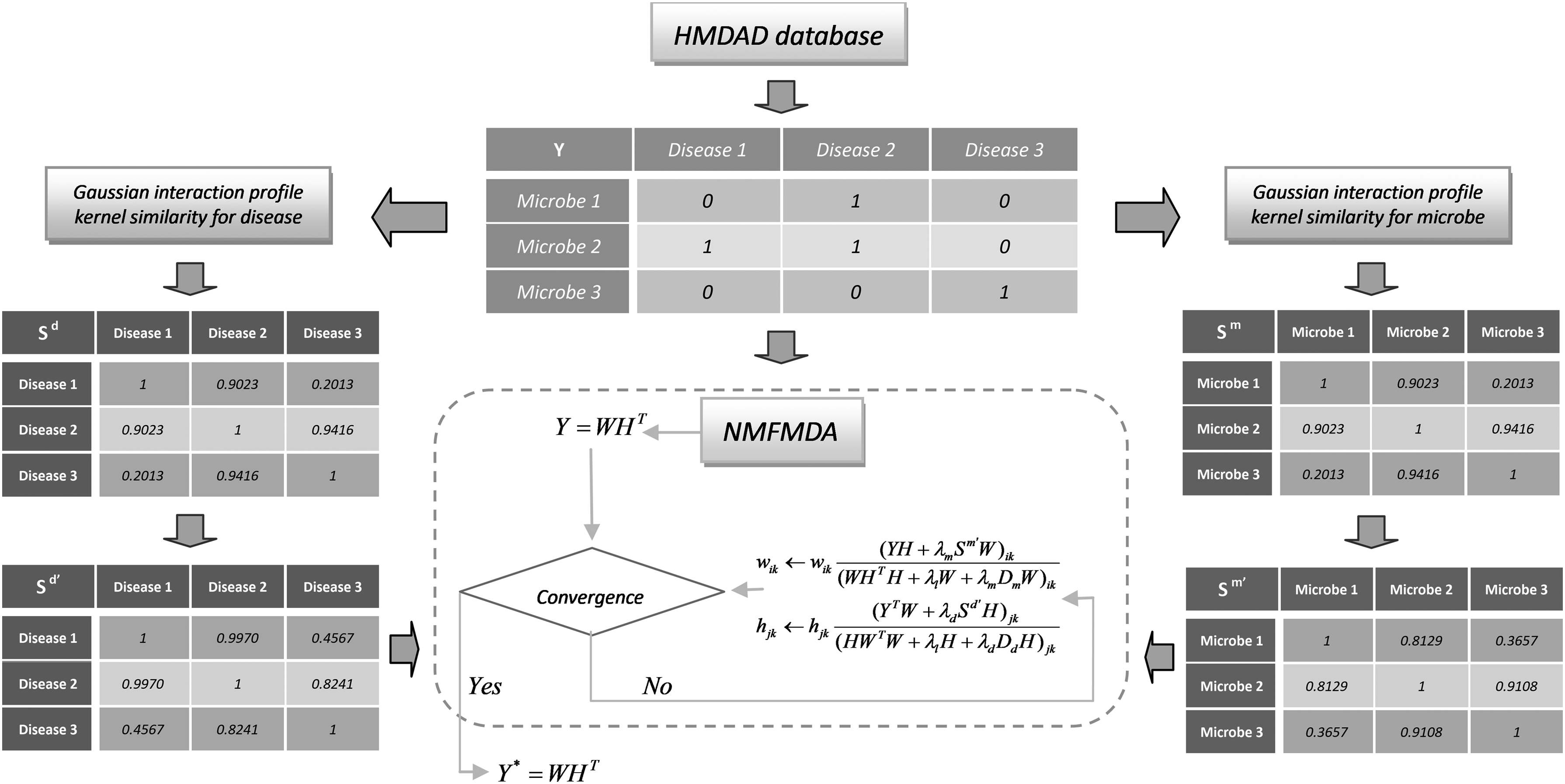
The NMFMDA method will be introduced in detail that mainly consists in the following three steps shown in Figure 1. First, Gaussian interaction profile kernel similarity measure was used to calculate disease–disease similarity and microbe–microbe similarity. Second, preprocessing the disease–disease similarity matrix and microbe–microbe similarity matrix. Finally, we decomposed the original adjacency matrix by graph-regularized non-negative matrix factorization.
Overall workflow of NMFMDA for discovering potential microbe–disease associations. HMDAD, human microbe–disease association database; NMFMDA, non-negative matrix factorization microbe–disease associations.
2.1. Disease similarity
In our approach, the microbe–microbe similarity matrix and the disease–disease similarity matrix need to be constructed separately, so we need to determine the similarity between each pair of disease–disease and each pair of microbe–microbe. We used Gaussian interaction profile nuclear similarity measure to calculate disease similarity and microbial similarity (van Laarhoven et al., 2011; Chen et al., 2016).
If a disease is associated with a certain type of microbe, diseases that have similar phenotypic characteristics to the disease are more likely to be associated with the microbe. Therefore, the Gaussian interaction profile nuclear similarity of microbes can be calculated from known microbe–disease association networks (Chen and Yan, 2013). We defined the binary vector \documentclass{aastex}\usepackage{amsbsy}\usepackage{amsfonts}\usepackage{amssymb}\usepackage{bm}\usepackage{mathrsfs}\usepackage{pifont}\usepackage{stmaryrd}\usepackage{textcomp}\usepackage{portland, xspace}\usepackage{amsmath, amsxtra}\usepackage{upgreek}\pagestyle{empty}\DeclareMathSizes{10}{9}{7}{6}\begin{document}
$$d \left( i \right)$$
\end{document} as the interaction profile of the disease di, the association with each microbe (the i-th row of the adjacency matrix Y). Then the Gaussian interaction profile nuclear similarity between disease \documentclass{aastex}\usepackage{amsbsy}\usepackage{amsfonts}\usepackage{amssymb}\usepackage{bm}\usepackage{mathrsfs}\usepackage{pifont}\usepackage{stmaryrd}\usepackage{textcomp}\usepackage{portland, xspace}\usepackage{amsmath, amsxtra}\usepackage{upgreek}\pagestyle{empty}\DeclareMathSizes{10}{9}{7}{6}\begin{document}
$$d \left( i \right)$$
\end{document} and \documentclass{aastex}\usepackage{amsbsy}\usepackage{amsfonts}\usepackage{amssymb}\usepackage{bm}\usepackage{mathrsfs}\usepackage{pifont}\usepackage{stmaryrd}\usepackage{textcomp}\usepackage{portland, xspace}\usepackage{amsmath, amsxtra}\usepackage{upgreek}\pagestyle{empty}\DeclareMathSizes{10}{9}{7}{6}\begin{document}
$$d \left( j \right)$$
\end{document} can be defined as follows:
\documentclass{aastex}\usepackage{amsbsy}\usepackage{amsfonts}\usepackage{amssymb}\usepackage{bm}\usepackage{mathrsfs}\usepackage{pifont}\usepackage{stmaryrd}\usepackage{textcomp}\usepackage{portland, xspace}\usepackage{amsmath, amsxtra}\usepackage{upgreek}\pagestyle{empty}\DeclareMathSizes{10}{9}{7}{6}\begin{document}
\begin{align*}
KD \left( {d \left( i \right) , d \left( j \right) } \right) = exp \left( { - { \gamma _d}{{ \left\vert \vert {d \left( i \right) - d \left( j \right) } \right\vert \vert }^2}} \right) , \tag{1}
\end{align*}
\end{document}
where \documentclass{aastex}\usepackage{amsbsy}\usepackage{amsfonts}\usepackage{amssymb}\usepackage{bm}\usepackage{mathrsfs}\usepackage{pifont}\usepackage{stmaryrd}\usepackage{textcomp}\usepackage{portland, xspace}\usepackage{amsmath, amsxtra}\usepackage{upgreek}\pagestyle{empty}\DeclareMathSizes{10}{9}{7}{6}\begin{document}
$${ \gamma _d}$$
\end{document} is responsible for controlling the kernel bandwidth. This parameter needs to be updated by the new kernel bandwidth parameter \documentclass{aastex}\usepackage{amsbsy}\usepackage{amsfonts}\usepackage{amssymb}\usepackage{bm}\usepackage{mathrsfs}\usepackage{pifont}\usepackage{stmaryrd}\usepackage{textcomp}\usepackage{portland, xspace}\usepackage{amsmath, amsxtra}\usepackage{upgreek}\pagestyle{empty}\DeclareMathSizes{10}{9}{7}{6}\begin{document}
$$\gamma _d^ \prime$$
\end{document}. The update rules are as follows:
\documentclass{aastex}\usepackage{amsbsy}\usepackage{amsfonts}\usepackage{amssymb}\usepackage{bm}\usepackage{mathrsfs}\usepackage{pifont}\usepackage{stmaryrd}\usepackage{textcomp}\usepackage{portland, xspace}\usepackage{amsmath, amsxtra}\usepackage{upgreek}\pagestyle{empty}\DeclareMathSizes{10}{9}{7}{6}\begin{document}
\begin{align*}
{ \gamma _d } = \gamma _d^ \prime / \left( { \frac { 1 } { { { n_d } } } \mathop \sum \limits_ { j = 1 } ^ { { n_d } } { { \left\vert \vert { d \left( i \right) } \right\vert \vert } ^2 } } \right) , \tag { 2 }
\end{align*}
\end{document}
where nd is the number of diseases. For calculation convenience, \documentclass{aastex}\usepackage{amsbsy}\usepackage{amsfonts}\usepackage{amssymb}\usepackage{bm}\usepackage{mathrsfs}\usepackage{pifont}\usepackage{stmaryrd}\usepackage{textcomp}\usepackage{portland, xspace}\usepackage{amsmath, amsxtra}\usepackage{upgreek}\pagestyle{empty}\DeclareMathSizes{10}{9}{7}{6}\begin{document}
$$\gamma _d^ \prime$$
\end{document} is set to 1 (Chen et al., 2017).
The disease similarity matrix \documentclass{aastex}\usepackage{amsbsy}\usepackage{amsfonts}\usepackage{amssymb}\usepackage{bm}\usepackage{mathrsfs}\usepackage{pifont}\usepackage{stmaryrd}\usepackage{textcomp}\usepackage{portland, xspace}\usepackage{amsmath, amsxtra}\usepackage{upgreek}\pagestyle{empty}\DeclareMathSizes{10}{9}{7}{6}\begin{document}
$${S^d} \in {R^{39 \times 39}}$$
\end{document} is constructed according to Equation (1).
2.2. Microbe similarity
Similar to diseases, Gaussian interaction profile kernel similarity between microbes \documentclass{aastex}\usepackage{amsbsy}\usepackage{amsfonts}\usepackage{amssymb}\usepackage{bm}\usepackage{mathrsfs}\usepackage{pifont}\usepackage{stmaryrd}\usepackage{textcomp}\usepackage{portland, xspace}\usepackage{amsmath, amsxtra}\usepackage{upgreek}\pagestyle{empty}\DeclareMathSizes{10}{9}{7}{6}\begin{document}
$$m \left( i \right)$$
\end{document} and \documentclass{aastex}\usepackage{amsbsy}\usepackage{amsfonts}\usepackage{amssymb}\usepackage{bm}\usepackage{mathrsfs}\usepackage{pifont}\usepackage{stmaryrd}\usepackage{textcomp}\usepackage{portland, xspace}\usepackage{amsmath, amsxtra}\usepackage{upgreek}\pagestyle{empty}\DeclareMathSizes{10}{9}{7}{6}\begin{document}
$$m \left( j \right)$$
\end{document} can be defined as follows:
\documentclass{aastex}\usepackage{amsbsy}\usepackage{amsfonts}\usepackage{amssymb}\usepackage{bm}\usepackage{mathrsfs}\usepackage{pifont}\usepackage{stmaryrd}\usepackage{textcomp}\usepackage{portland, xspace}\usepackage{amsmath, amsxtra}\usepackage{upgreek}\pagestyle{empty}\DeclareMathSizes{10}{9}{7}{6}\begin{document}
\begin{align*}
KM \left( {m \left( i \right) , m \left( j \right) } \right) = exp \left( { - { \gamma _m}{{ \left\vert \vert {m \left( i \right) - m \left( j \right) } \right\vert \vert }^2}} \right) , \tag{3}
\end{align*}
\end{document}
where \documentclass{aastex}\usepackage{amsbsy}\usepackage{amsfonts}\usepackage{amssymb}\usepackage{bm}\usepackage{mathrsfs}\usepackage{pifont}\usepackage{stmaryrd}\usepackage{textcomp}\usepackage{portland, xspace}\usepackage{amsmath, amsxtra}\usepackage{upgreek}\pagestyle{empty}\DeclareMathSizes{10}{9}{7}{6}\begin{document}
$${ \gamma _m}$$
\end{document} is responsible for controlling the kernel bandwidth. The update rules are as follows:
\documentclass{aastex}\usepackage{amsbsy}\usepackage{amsfonts}\usepackage{amssymb}\usepackage{bm}\usepackage{mathrsfs}\usepackage{pifont}\usepackage{stmaryrd}\usepackage{textcomp}\usepackage{portland, xspace}\usepackage{amsmath, amsxtra}\usepackage{upgreek}\pagestyle{empty}\DeclareMathSizes{10}{9}{7}{6}\begin{document}
\begin{align*}
{ \gamma _m } = \gamma _m^ \prime / \left( { \frac { 1 } { { { n_m } } } \mathop \sum \limits_ { j = 1 } ^ { { n_m } } { { \left\vert \vert { m \left( i \right) } \right\vert \vert } ^2 } } \right) , \tag { 4 }
\end{align*}
\end{document}
where nm is the number of microbes. For calculation convenience, \documentclass{aastex}\usepackage{amsbsy}\usepackage{amsfonts}\usepackage{amssymb}\usepackage{bm}\usepackage{mathrsfs}\usepackage{pifont}\usepackage{stmaryrd}\usepackage{textcomp}\usepackage{portland, xspace}\usepackage{amsmath, amsxtra}\usepackage{upgreek}\pagestyle{empty}\DeclareMathSizes{10}{9}{7}{6}\begin{document}
$$\gamma _m^ \prime$$
\end{document} is set to 1.
The microbial similarity matrix \documentclass{aastex}\usepackage{amsbsy}\usepackage{amsfonts}\usepackage{amssymb}\usepackage{bm}\usepackage{mathrsfs}\usepackage{pifont}\usepackage{stmaryrd}\usepackage{textcomp}\usepackage{portland, xspace}\usepackage{amsmath, amsxtra}\usepackage{upgreek}\pagestyle{empty}\DeclareMathSizes{10}{9}{7}{6}\begin{document}
$${S^m} \in {R^{292 \times 292}}$$
\end{document} is constructed according to Equation (3).
2.3. Matrix preprocessing
Because our method needs to operate on the processed Sd and Sm, we first preprocess these two matrices to facilitate later calculations.
Spectral graph and manifold learning theories proved that local geometric structures can be effectively modeled by the scattered nearest neighbors of data points (Cai et al., 2011). Microbes in the same cluster are often more similar, and diseases are the same. Based on the p nearest neighbor clustering, we constructed the graphs (\documentclass{aastex}\usepackage{amsbsy}\usepackage{amsfonts}\usepackage{amssymb}\usepackage{bm}\usepackage{mathrsfs}\usepackage{pifont}\usepackage{stmaryrd}\usepackage{textcomp}\usepackage{portland, xspace}\usepackage{amsmath, amsxtra}\usepackage{upgreek}\pagestyle{empty}\DeclareMathSizes{10}{9}{7}{6}\begin{document}
$${S^{d \prime }}$$
\end{document} and \documentclass{aastex}\usepackage{amsbsy}\usepackage{amsfonts}\usepackage{amssymb}\usepackage{bm}\usepackage{mathrsfs}\usepackage{pifont}\usepackage{stmaryrd}\usepackage{textcomp}\usepackage{portland, xspace}\usepackage{amsmath, amsxtra}\usepackage{upgreek}\pagestyle{empty}\DeclareMathSizes{10}{9}{7}{6}\begin{document}
$${S^{m \prime }}$$
\end{document}) for microbes and diseases, respectively, using ClusterONE (Nepusz et al., 2012). The weight matrix Xm is generated based on the microbial similarity matrix Sm as follows:
where \documentclass{aastex}\usepackage{amsbsy}\usepackage{amsfonts}\usepackage{amssymb}\usepackage{bm}\usepackage{mathrsfs}\usepackage{pifont}\usepackage{stmaryrd}\usepackage{textcomp}\usepackage{portland, xspace}\usepackage{amsmath, amsxtra}\usepackage{upgreek}\pagestyle{empty}\DeclareMathSizes{10}{9}{7}{6}\begin{document}
$$N \left( {{m_i}} \right)$$
\end{document} and \documentclass{aastex}\usepackage{amsbsy}\usepackage{amsfonts}\usepackage{amssymb}\usepackage{bm}\usepackage{mathrsfs}\usepackage{pifont}\usepackage{stmaryrd}\usepackage{textcomp}\usepackage{portland, xspace}\usepackage{amsmath, amsxtra}\usepackage{upgreek}\pagestyle{empty}\DeclareMathSizes{10}{9}{7}{6}\begin{document}
$$N \left( {{m_j}} \right)$$
\end{document} are the set of p nearest neighbors of mi and mj, and C represents any cluster after cluster. Thus, matrix \documentclass{aastex}\usepackage{amsbsy}\usepackage{amsfonts}\usepackage{amssymb}\usepackage{bm}\usepackage{mathrsfs}\usepackage{pifont}\usepackage{stmaryrd}\usepackage{textcomp}\usepackage{portland, xspace}\usepackage{amsmath, amsxtra}\usepackage{upgreek}\pagestyle{empty}\DeclareMathSizes{10}{9}{7}{6}\begin{document}
$${S^{m \prime }}$$
\end{document} for microbes is defined as
\documentclass{aastex}\usepackage{amsbsy}\usepackage{amsfonts}\usepackage{amssymb}\usepackage{bm}\usepackage{mathrsfs}\usepackage{pifont}\usepackage{stmaryrd}\usepackage{textcomp}\usepackage{portland, xspace}\usepackage{amsmath, amsxtra}\usepackage{upgreek}\pagestyle{empty}\DeclareMathSizes{10}{9}{7}{6}\begin{document}
\begin{align*}
\forall i , jS_{ij}^{m \prime } = X_{ij}^mS_{ij}^m. \tag{6}
\end{align*}
\end{document}
Similarly, matrix \documentclass{aastex}\usepackage{amsbsy}\usepackage{amsfonts}\usepackage{amssymb}\usepackage{bm}\usepackage{mathrsfs}\usepackage{pifont}\usepackage{stmaryrd}\usepackage{textcomp}\usepackage{portland, xspace}\usepackage{amsmath, amsxtra}\usepackage{upgreek}\pagestyle{empty}\DeclareMathSizes{10}{9}{7}{6}\begin{document}
$${S^{d \prime }}$$
\end{document} for diseases is available.
The non-negative matrix factorization algorithm is widely used to process data in various fields. This algorithm decomposes a large original matrix into two matrices to achieve the purpose of dimension reduction and matrix data filling. In our method, the original microbe–disease similarity matrix \documentclass{aastex}\usepackage{amsbsy}\usepackage{amsfonts}\usepackage{amssymb}\usepackage{bm}\usepackage{mathrsfs}\usepackage{pifont}\usepackage{stmaryrd}\usepackage{textcomp}\usepackage{portland, xspace}\usepackage{amsmath, amsxtra}\usepackage{upgreek}\pagestyle{empty}\DeclareMathSizes{10}{9}{7}{6}\begin{document}
$$Y \in {R^{292 \times 39}}$$
\end{document} (where \documentclass{aastex}\usepackage{amsbsy}\usepackage{amsfonts}\usepackage{amssymb}\usepackage{bm}\usepackage{mathrsfs}\usepackage{pifont}\usepackage{stmaryrd}\usepackage{textcomp}\usepackage{portland, xspace}\usepackage{amsmath, amsxtra}\usepackage{upgreek}\pagestyle{empty}\DeclareMathSizes{10}{9}{7}{6}\begin{document}
$${Y_{ij}} = 1$$
\end{document} if microbe mi has a known association with disease dj, otherwise \documentclass{aastex}\usepackage{amsbsy}\usepackage{amsfonts}\usepackage{amssymb}\usepackage{bm}\usepackage{mathrsfs}\usepackage{pifont}\usepackage{stmaryrd}\usepackage{textcomp}\usepackage{portland, xspace}\usepackage{amsmath, amsxtra}\usepackage{upgreek}\pagestyle{empty}\DeclareMathSizes{10}{9}{7}{6}\begin{document}
$${Y_{ij}} = 0$$
\end{document}) is decomposed into W and H (\documentclass{aastex}\usepackage{amsbsy}\usepackage{amsfonts}\usepackage{amssymb}\usepackage{bm}\usepackage{mathrsfs}\usepackage{pifont}\usepackage{stmaryrd}\usepackage{textcomp}\usepackage{portland, xspace}\usepackage{amsmath, amsxtra}\usepackage{upgreek}\pagestyle{empty}\DeclareMathSizes{10}{9}{7}{6}\begin{document}
$$Y = W{H^T}$$
\end{document}), that is \documentclass{aastex}\usepackage{amsbsy}\usepackage{amsfonts}\usepackage{amssymb}\usepackage{bm}\usepackage{mathrsfs}\usepackage{pifont}\usepackage{stmaryrd}\usepackage{textcomp}\usepackage{portland, xspace}\usepackage{amsmath, amsxtra}\usepackage{upgreek}\pagestyle{empty}\DeclareMathSizes{10}{9}{7}{6}\begin{document}
$$W \in {R^{292 \times k}}$$
\end{document}, \documentclass{aastex}\usepackage{amsbsy}\usepackage{amsfonts}\usepackage{amssymb}\usepackage{bm}\usepackage{mathrsfs}\usepackage{pifont}\usepackage{stmaryrd}\usepackage{textcomp}\usepackage{portland, xspace}\usepackage{amsmath, amsxtra}\usepackage{upgreek}\pagestyle{empty}\DeclareMathSizes{10}{9}{7}{6}\begin{document}
$$H \in {R^{k \times 39}}$$
\end{document} (where k is the subspace dimension).
Li's study shows that the standard non-negative matrix factorization cannot discover the intrinsic geometrical and discriminating structure of the data space in the Euclidean space (Li et al., 2017b). To prevent overfitting and to significantly enhance the learning performance, we presented a new objective function through incorporation of the Tikhonov (L2) and graph Laplacian regularization terms into the standard non-negative matrix factorization framework for microbe–disease association prediction. The Tikhonov regularization is used to ensure the W and H smoothness (Guan et al., 2011), and the graph regularization mainly aims to guarantee a part-based representation by fully exploiting the data geometric structure (Cai et al., 2011). The definition of the objective function of my graph regularization non-negative matrix factorization is as follows:
\documentclass{aastex}\usepackage{amsbsy}\usepackage{amsfonts}\usepackage{amssymb}\usepackage{bm}\usepackage{mathrsfs}\usepackage{pifont}\usepackage{stmaryrd}\usepackage{textcomp}\usepackage{portland, xspace}\usepackage{amsmath, amsxtra}\usepackage{upgreek}\pagestyle{empty}\DeclareMathSizes{10}{9}{7}{6}\begin{document}
\begin{align*}
\begin{split} & \mathop { \min } \limits_{W , H} \left\vert \vert {Y - W{H^T}} \right\vert \vert _F^2 + { \lambda _l} \left( { \left\vert \vert W \right\vert \vert _F^2 + \left\vert \vert H \right\vert \vert _F^2} \right) + { \lambda _m} \mathop \sum \limits_{i , p = 1}^n { \left\vert \vert {{w_i} - {w_p}} \right\vert \vert ^2}S_{ip}^{m \prime } + { \lambda _d} \mathop \sum \limits_{j , q = 1}^m { \left\vert \vert {{h_j} - {h_q}} \right\vert \vert ^2}S_{jq}^{d \prime } \\ & s.t.W \ge 0 , H \ge 0 \\ ,\end{split} \tag{7}
\end{align*}
\end{document}
where \documentclass{aastex}\usepackage{amsbsy}\usepackage{amsfonts}\usepackage{amssymb}\usepackage{bm}\usepackage{mathrsfs}\usepackage{pifont}\usepackage{stmaryrd}\usepackage{textcomp}\usepackage{portland, xspace}\usepackage{amsmath, amsxtra}\usepackage{upgreek}\pagestyle{empty}\DeclareMathSizes{10}{9}{7}{6}\begin{document}
$${ \lambda _l}$$
\end{document}, \documentclass{aastex}\usepackage{amsbsy}\usepackage{amsfonts}\usepackage{amssymb}\usepackage{bm}\usepackage{mathrsfs}\usepackage{pifont}\usepackage{stmaryrd}\usepackage{textcomp}\usepackage{portland, xspace}\usepackage{amsmath, amsxtra}\usepackage{upgreek}\pagestyle{empty}\DeclareMathSizes{10}{9}{7}{6}\begin{document}
$${ \lambda _d}$$
\end{document}, and \documentclass{aastex}\usepackage{amsbsy}\usepackage{amsfonts}\usepackage{amssymb}\usepackage{bm}\usepackage{mathrsfs}\usepackage{pifont}\usepackage{stmaryrd}\usepackage{textcomp}\usepackage{portland, xspace}\usepackage{amsmath, amsxtra}\usepackage{upgreek}\pagestyle{empty}\DeclareMathSizes{10}{9}{7}{6}\begin{document}
$${ \lambda _m}$$
\end{document} are regularization coefficients. wi and hj are the i-th and j-th rows of w and h. The mentioned equation can be transformed to
\documentclass{aastex}\usepackage{amsbsy}\usepackage{amsfonts}\usepackage{amssymb}\usepackage{bm}\usepackage{mathrsfs}\usepackage{pifont}\usepackage{stmaryrd}\usepackage{textcomp}\usepackage{portland, xspace}\usepackage{amsmath, amsxtra}\usepackage{upgreek}\pagestyle{empty}\DeclareMathSizes{10}{9}{7}{6}\begin{document}
\begin{align*}
\begin{split} & \mathop { \min } \limits_{W , H} \left\vert \vert {Y - W{H^T}} \right\vert \vert _F^2 + { \lambda _l} \left( { \left\vert \vert W \right\vert \vert _F^2 + \left\vert \vert H \right\vert \vert _F^2} \right) + { \lambda _m}Tr \left( {{W^T}{L_m}W} \right) + { \lambda _d}Tr \left( {{H^T}{L_d}H} \right) \\ & s.t.W \ge 0 , H \ge 0 \\ ,\end{split} \tag{8}
\end{align*}
\end{document}
where \documentclass{aastex}\usepackage{amsbsy}\usepackage{amsfonts}\usepackage{amssymb}\usepackage{bm}\usepackage{mathrsfs}\usepackage{pifont}\usepackage{stmaryrd}\usepackage{textcomp}\usepackage{portland, xspace}\usepackage{amsmath, amsxtra}\usepackage{upgreek}\pagestyle{empty}\DeclareMathSizes{10}{9}{7}{6}\begin{document}
$$Tr \left(. \right)$$
\end{document} is the trace of a matrix and Lm and Ld are the graph Laplacian matrices for \documentclass{aastex}\usepackage{amsbsy}\usepackage{amsfonts}\usepackage{amssymb}\usepackage{bm}\usepackage{mathrsfs}\usepackage{pifont}\usepackage{stmaryrd}\usepackage{textcomp}\usepackage{portland, xspace}\usepackage{amsmath, amsxtra}\usepackage{upgreek}\pagestyle{empty}\DeclareMathSizes{10}{9}{7}{6}\begin{document}
$${S^{m \prime }}$$
\end{document} and \documentclass{aastex}\usepackage{amsbsy}\usepackage{amsfonts}\usepackage{amssymb}\usepackage{bm}\usepackage{mathrsfs}\usepackage{pifont}\usepackage{stmaryrd}\usepackage{textcomp}\usepackage{portland, xspace}\usepackage{amsmath, amsxtra}\usepackage{upgreek}\pagestyle{empty}\DeclareMathSizes{10}{9}{7}{6}\begin{document}
$${S^{d \prime }}$$
\end{document} (\documentclass{aastex}\usepackage{amsbsy}\usepackage{amsfonts}\usepackage{amssymb}\usepackage{bm}\usepackage{mathrsfs}\usepackage{pifont}\usepackage{stmaryrd}\usepackage{textcomp}\usepackage{portland, xspace}\usepackage{amsmath, amsxtra}\usepackage{upgreek}\pagestyle{empty}\DeclareMathSizes{10}{9}{7}{6}\begin{document}
$${L_d} = {D_d} - {S^{d \prime }}$$
\end{document} and \documentclass{aastex}\usepackage{amsbsy}\usepackage{amsfonts}\usepackage{amssymb}\usepackage{bm}\usepackage{mathrsfs}\usepackage{pifont}\usepackage{stmaryrd}\usepackage{textcomp}\usepackage{portland, xspace}\usepackage{amsmath, amsxtra}\usepackage{upgreek}\pagestyle{empty}\DeclareMathSizes{10}{9}{7}{6}\begin{document}
$${L_m} = {D_m} - {S^{m \prime }}$$
\end{document}), where Dd and Dm are the diagonal matrices whose entries are row (or column) sums of \documentclass{aastex}\usepackage{amsbsy}\usepackage{amsfonts}\usepackage{amssymb}\usepackage{bm}\usepackage{mathrsfs}\usepackage{pifont}\usepackage{stmaryrd}\usepackage{textcomp}\usepackage{portland, xspace}\usepackage{amsmath, amsxtra}\usepackage{upgreek}\pagestyle{empty}\DeclareMathSizes{10}{9}{7}{6}\begin{document}
$${S^{m \prime }}$$
\end{document}and \documentclass{aastex}\usepackage{amsbsy}\usepackage{amsfonts}\usepackage{amssymb}\usepackage{bm}\usepackage{mathrsfs}\usepackage{pifont}\usepackage{stmaryrd}\usepackage{textcomp}\usepackage{portland, xspace}\usepackage{amsmath, amsxtra}\usepackage{upgreek}\pagestyle{empty}\DeclareMathSizes{10}{9}{7}{6}\begin{document}
$${S^{d \prime }}$$
\end{document}, respectively.
We used the method of derivation of the Lagrange function to optimize the objective function, and sought the most suitable matrix of W and H, respectively. The following update rules are available:
\documentclass{aastex}\usepackage{amsbsy}\usepackage{amsfonts}\usepackage{amssymb}\usepackage{bm}\usepackage{mathrsfs}\usepackage{pifont}\usepackage{stmaryrd}\usepackage{textcomp}\usepackage{portland, xspace}\usepackage{amsmath, amsxtra}\usepackage{upgreek}\pagestyle{empty}\DeclareMathSizes{10}{9}{7}{6}\begin{document}
\begin{align*}
{ w_ { ik } } \leftarrow { w_ { ik } } { \frac { { { \left( { YH + { \lambda _m } { S^ { m \prime } } W } \right) } _ { ik } } } { { { \left( { W { H^T } H + { \lambda _l } W + { \lambda _m } { D_m } W } \right) } _ { ik } } } } , \tag { 9 }
\end{align*}
\end{document}\documentclass{aastex}\usepackage{amsbsy}\usepackage{amsfonts}\usepackage{amssymb}\usepackage{bm}\usepackage{mathrsfs}\usepackage{pifont}\usepackage{stmaryrd}\usepackage{textcomp}\usepackage{portland, xspace}\usepackage{amsmath, amsxtra}\usepackage{upgreek}\pagestyle{empty}\DeclareMathSizes{10}{9}{7}{6}\begin{document}
\begin{align*}
{ h_ { jk } } \leftarrow { h_ { jk } } { \frac { { { \left( { { Y^T } W + { \lambda _d } { S^ { d \prime } } H } \right) } _ { jk } } } { { { \left( { H { W^T } W + { \lambda _l } H + { \lambda _d } { D_d } H } \right) } _ { jk } } } } , \tag { 10 }
\end{align*}
\end{document}
where matrices W and H are updated according to the described update rules until convergence or reaching the iteration upper limit. Finally, the new \documentclass{aastex}\usepackage{amsbsy}\usepackage{amsfonts}\usepackage{amssymb}\usepackage{bm}\usepackage{mathrsfs}\usepackage{pifont}\usepackage{stmaryrd}\usepackage{textcomp}\usepackage{portland, xspace}\usepackage{amsmath, amsxtra}\usepackage{upgreek}\pagestyle{empty}\DeclareMathSizes{10}{9}{7}{6}\begin{document}
$${Y^*}$$
\end{document} that we multiply by W and HT is the final result. Each entry represents the probability that the disease is related to the microbe. The first few sorted results for each column are the microbes most affected by the disease. Table 1 summarizes the procedure of NMFMDA for microbe–disease association prediction.
Algorithm Description of Non-Negative Matrix Factorization Microbe–Disease Associations
The operational environment of experiment in this article is as follows: Window 7 operating system, the RAM is 16GB, and the speed of processor is 3.5 GHz. The algorithm runs on the software Matlab R2016a.
3.1. Data sets
The database explored in this work was downloaded from the HMDAD (www.cuilab.cn/hmdad; Ma et al., 2017). It integrated 483 high-quality microbe–disease entries, which were mainly collected from 16S RNA sequencing-based microbial literature. After removing the duplicate association records, 450 distinct microbe–disease associations were finally obtained, including 292 microbes and 39 diseases. We used these data to construct microbe–disease adjacency matrix \documentclass{aastex}\usepackage{amsbsy}\usepackage{amsfonts}\usepackage{amssymb}\usepackage{bm}\usepackage{mathrsfs}\usepackage{pifont}\usepackage{stmaryrd}\usepackage{textcomp}\usepackage{portland, xspace}\usepackage{amsmath, amsxtra}\usepackage{upgreek}\pagestyle{empty}\DeclareMathSizes{10}{9}{7}{6}\begin{document}
$$Y \in {R^{292 \times 39}}$$
\end{document}.
3.2. Performance evaluation
To evaluate the performance of our model, we used fivefold cross-validation. In the framework of fivefold cross-validation, 450 known relational samples were randomly divided into five groups. For each trial, one group was used as the test set and the other four groups were used as the training set (Zou et al., 2014). Moreover, to reduce the chance of data partitioning, we conducted 100 trials. Our result was the average of these 100 trials.
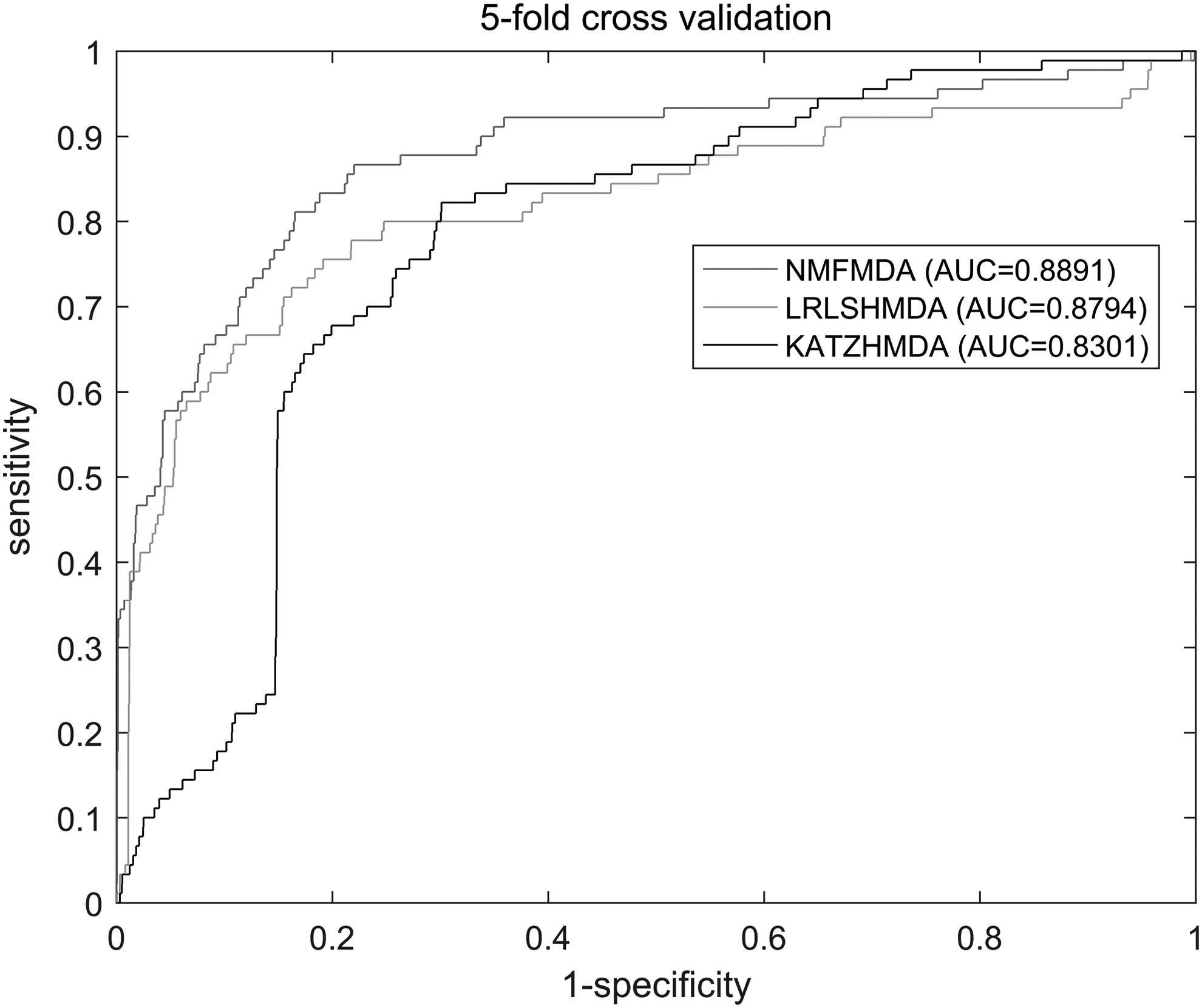
The receiver operating characteristic (ROC) curve was plotted by setting different thresholds. The abscissa of the ROC curve is 1-specificity (false positive rate) and the ordinate is sensitivity (true positive rate). Sensitivity represents the percentage of test samples ranked more than a given threshold, whereas specificity indicates the opposite. The ROC curve is obtained and the AUC value can be calculated accordingly. If AUC = 1 indicates perfect performance, AUC = 0.5 indicates random performance. According to our experimental results, the result of fivefold cross-validation is 0.8891, which confirms the superior performance of our method.
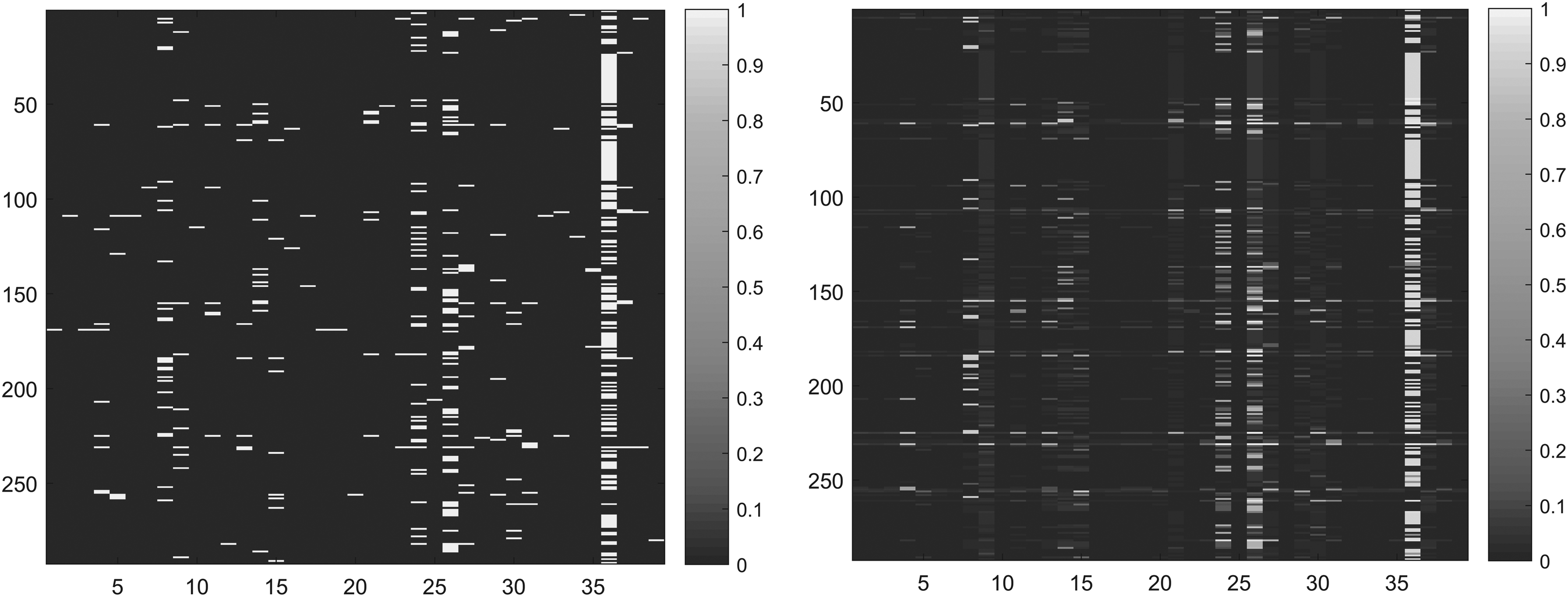
It is known that KATZHMDA (KATZ measure for human microbe-disease association) and LLRSHMDA (Laplacian regularized least squares for human microbe-disease association) are state-of-the-art methods for predicting the similarity of microbes and diseases (Katz, 1952). KATZHMDA is based on the KATZ measure that calculates nodes' similarity in the heterogeneous network to calculate microbe–disease similarity (Chen et al., 2017); the LLRSHMDA used Laplacian-regularized least squares classifier to predict microbe–disease similarity (Wang et al., 2017). Similar to our method, using the HMDAD database, based on the network of known microbe–disease similarity, their AUCs are 0.8301 and 0.8794, respectively. The results show that our NMFMDA is better than other methods. Figure 2 shows the ROC curves for the three methods. Figure 3 shows the comparison of the initial adjacency matrix and the result matrix. Larger values indicate that the disease and this microbe are more likely to be similar.
The ROC curves for the three methods. AUC, area under receiver operating characteristic curve; ROC, receiver operating characteristic.
The comparison of the initial adjacency matrix (left) and the result matrix (right).
3.3. Effect of parameters
We determined the best parameters based on cross-validation results. All parameters are based on grid search. Our model has the following parameters: subspace dimensionality k, regularization coefficients \documentclass{aastex}\usepackage{amsbsy}\usepackage{amsfonts}\usepackage{amssymb}\usepackage{bm}\usepackage{mathrsfs}\usepackage{pifont}\usepackage{stmaryrd}\usepackage{textcomp}\usepackage{portland, xspace}\usepackage{amsmath, amsxtra}\usepackage{upgreek}\pagestyle{empty}\DeclareMathSizes{10}{9}{7}{6}\begin{document}
$${ \lambda _l}$$
\end{document}, \documentclass{aastex}\usepackage{amsbsy}\usepackage{amsfonts}\usepackage{amssymb}\usepackage{bm}\usepackage{mathrsfs}\usepackage{pifont}\usepackage{stmaryrd}\usepackage{textcomp}\usepackage{portland, xspace}\usepackage{amsmath, amsxtra}\usepackage{upgreek}\pagestyle{empty}\DeclareMathSizes{10}{9}{7}{6}\begin{document}
$${ \lambda _d}$$
\end{document}, \documentclass{aastex}\usepackage{amsbsy}\usepackage{amsfonts}\usepackage{amssymb}\usepackage{bm}\usepackage{mathrsfs}\usepackage{pifont}\usepackage{stmaryrd}\usepackage{textcomp}\usepackage{portland, xspace}\usepackage{amsmath, amsxtra}\usepackage{upgreek}\pagestyle{empty}\DeclareMathSizes{10}{9}{7}{6}\begin{document}
$${ \lambda _m}$$
\end{document}, and neighborhood size p. Experiments show that the value of k does not have a great influence on the result, and the effect is best when k = 38. The range of \documentclass{aastex}\usepackage{amsbsy}\usepackage{amsfonts}\usepackage{amssymb}\usepackage{bm}\usepackage{mathrsfs}\usepackage{pifont}\usepackage{stmaryrd}\usepackage{textcomp}\usepackage{portland, xspace}\usepackage{amsmath, amsxtra}\usepackage{upgreek}\pagestyle{empty}\DeclareMathSizes{10}{9}{7}{6}\begin{document}
$${ \lambda _l}$$
\end{document} is {0.6 0.8 1.0 1.2}. The range of \documentclass{aastex}\usepackage{amsbsy}\usepackage{amsfonts}\usepackage{amssymb}\usepackage{bm}\usepackage{mathrsfs}\usepackage{pifont}\usepackage{stmaryrd}\usepackage{textcomp}\usepackage{portland, xspace}\usepackage{amsmath, amsxtra}\usepackage{upgreek}\pagestyle{empty}\DeclareMathSizes{10}{9}{7}{6}\begin{document}
$${ \lambda _d}$$
\end{document} = \documentclass{aastex}\usepackage{amsbsy}\usepackage{amsfonts}\usepackage{amssymb}\usepackage{bm}\usepackage{mathrsfs}\usepackage{pifont}\usepackage{stmaryrd}\usepackage{textcomp}\usepackage{portland, xspace}\usepackage{amsmath, amsxtra}\usepackage{upgreek}\pagestyle{empty}\DeclareMathSizes{10}{9}{7}{6}\begin{document}
$${ \lambda _m}$$
\end{document} is {0.6 0.8 1.0 1.2}. Based on the study of Cai et al. (2011), the value of p is 5 (Li et al., 2017b). Table 2 lists the AUC values of these combinations. Experiments show that the best value of \documentclass{aastex}\usepackage{amsbsy}\usepackage{amsfonts}\usepackage{amssymb}\usepackage{bm}\usepackage{mathrsfs}\usepackage{pifont}\usepackage{stmaryrd}\usepackage{textcomp}\usepackage{portland, xspace}\usepackage{amsmath, amsxtra}\usepackage{upgreek}\pagestyle{empty}\DeclareMathSizes{10}{9}{7}{6}\begin{document}
$${ \lambda _l}$$
\end{document}, \documentclass{aastex}\usepackage{amsbsy}\usepackage{amsfonts}\usepackage{amssymb}\usepackage{bm}\usepackage{mathrsfs}\usepackage{pifont}\usepackage{stmaryrd}\usepackage{textcomp}\usepackage{portland, xspace}\usepackage{amsmath, amsxtra}\usepackage{upgreek}\pagestyle{empty}\DeclareMathSizes{10}{9}{7}{6}\begin{document}
$${ \lambda _d}$$
\end{document}, and \documentclass{aastex}\usepackage{amsbsy}\usepackage{amsfonts}\usepackage{amssymb}\usepackage{bm}\usepackage{mathrsfs}\usepackage{pifont}\usepackage{stmaryrd}\usepackage{textcomp}\usepackage{portland, xspace}\usepackage{amsmath, amsxtra}\usepackage{upgreek}\pagestyle{empty}\DeclareMathSizes{10}{9}{7}{6}\begin{document}
$${ \lambda _m}$$
\end{document} are 0.6, 0.8, and 0.8, respectively.
Effect of Parameters \documentclass{aastex}\usepackage{amsbsy}\usepackage{amsfonts}\usepackage{amssymb}\usepackage{bm}\usepackage{mathrsfs}\usepackage{pifont}\usepackage{stmaryrd}\usepackage{textcomp}\usepackage{portland, xspace}\usepackage{amsmath, amsxtra}\usepackage{upgreek}\pagestyle{empty}\DeclareMathSizes{10}{9}{7}{6}\begin{document}
$${ \lambda _l}$$
\end{document}, \documentclass{aastex}\usepackage{amsbsy}\usepackage{amsfonts}\usepackage{amssymb}\usepackage{bm}\usepackage{mathrsfs}\usepackage{pifont}\usepackage{stmaryrd}\usepackage{textcomp}\usepackage{portland, xspace}\usepackage{amsmath, amsxtra}\usepackage{upgreek}\pagestyle{empty}\DeclareMathSizes{10}{9}{7}{6}\begin{document}
$${ \lambda _d}$$
\end{document}, and \documentclass{aastex}\usepackage{amsbsy}\usepackage{amsfonts}\usepackage{amssymb}\usepackage{bm}\usepackage{mathrsfs}\usepackage{pifont}\usepackage{stmaryrd}\usepackage{textcomp}\usepackage{portland, xspace}\usepackage{amsmath, amsxtra}\usepackage{upgreek}\pagestyle{empty}\DeclareMathSizes{10}{9}{7}{6}\begin{document}
$${ \lambda _m}$$
\end{document} in the Results
To further evaluate the model, we conducted a separate case study of three complex human diseases (i.e., asthma, IBD, and colon cancer), respectively. According to recent literature and clinical trials, the top 10, 9, and 9 microbes of these three diseases were separately verified. It should be noted that the top 10 rankings we refer to are the rankings of the experimental results after removing the HMDAD known associated data, which guarantees absolute independence between the verified candidates and the known associations used for model training.
3.4.1. Asthma
Asthma is a common inflammatory disease. In our prediction results, the top 10 microbes have been verified. The proportion of firmicutes (first in the prediction list) and Actinobacteria (third in the prediction list) was found to be lower in asthmatic patients than in nonasthmatic people (Stokholm et al., 2018). Colonization by clostridium difficile (second in the prediction list) at 1 month of age correlates with the incidence of asthma between 6 and 7 years of age (van Nimwegen et al., 2011). Lactobacillus could inhibit airway inflammation in an ovalbumin-induced murine model of asthma (Yu et al., 2010). The top 10 candidate microbes of asthma obtained by our method are also listed in Table 3, all of them have been confirmed by the existing literature.
Effect in the Case Study of Asthma, All of Top-10 Predicted Microbes Have Been Supported by Literature Evidence
IBD is inflammation of the small intestine and colon. In NMFMDA, 9 of the top 10 microbes associated with IBD have been confirmed. Bacteroidetes (first in the prediction list), firmicutes (second in the prediction list), and Prevotella have been shown to be associated with IBD through the Kruskal–Wallis test (Walters et al., 2014). The helicobacter pylori is negatively correlated with IBD (Zeng et al., 2016). The top 10 candidate microbes for IBD obtained from NMFMDA are also listed in Table 4.
Effect in the Case Study of Inflammatory Bowel Disease, 9 of Top-10 Predicted Microbes Have Been Supported by Literature Evidence
Rank
Microbes
Evidence
1
Bacteroidetes
PMID:25307765
2
Firmicutes
PMID:25307765
3
Staphylococcus
PMID:23679203
4
Prevotella
PMID:25307765
5
Helicobacter pylori
PMID:22221289
6
Veillonella
PMID:24013298
7
Clostridium coccoides
PMID:19235886
8
Clostridium difficile
Azimirad et al. (2012)
9
Enteroloacteriaceae
Xochitl et al. (2012)
10
Haemophilus
Unconfirmed
3.4.3. Colon cancer
Colon cancer is a disease with a high incidence. We have predicted colon cancer-related microbes. Nine of the top 10 microbes have been confirmed by existing biological literature. Typically, it is reported that colon cancer patients aged 60 years or older who have inserted a metal stent preoperatively are identified as a risk factor for Clostridium difficile (first in the prediction list) infection (Li et al., 2017a). Helicobacter pylori (second in the prediction list) infection was found to be associated with risk increase of left-sided colon cancer (Zhang et al., 2012). By sequencing of 16S rRNA gene V3 region, abundance of Proteobacteria (third in the prediction list) was discovered under-represented in sporadic colon cancer patients (Gao et al., 2015). The top 10 candidate microbes for colon cancer obtained from NMFMDA are also listed in Table 5.
Effect in the Case Study of Colon Cancer, 9 of Top-10 Predicted Microbes Have Been Supported by Literature Evidence
Rank
Microbes
Evidence
1
Clostridium difficile
PMID:21152135
2
Helicobacter pylori
PMID:22294430
3
Proteobacteria
PMID:25699023
4
Bacteroidetes
PMID:25699024
5
Staphylococcus aureus
Unconfirmed
6
Prevotella
PMID:25699024
7
Firmicutes
PMID:25699024
8
Clostridium coccoides
PMID:18237311
9
Haemophilus
PMID:22761885
10
Lactobacillus
PMID:15828052
4. Conclusion
A large number of studies have shown that microbes have a particularly important relationship with human health and disease. The exploration of the relationship between diseases and microbes not only enables people to better understand the pathogenesis but also helps in the diagnosis and prevention of diseases. However, few people are committed to the prediction of large-scale disease and microbe relationships. Therefore, we proposed a new method called NMFDMA based on HMDAD to predict the relationship between them. NMFDMA uses the Gaussian interaction profile nuclear similarity to measure the disease–disease similarity and microbe–microbe similarity. And, a graph-regularized non-negative matrix factorization model was utilized to simultaneously identify potential microbe–disease associations. Fivefold cross-validation was used to measure the performance of our method. NMFDMA achieved a 0.8891 AUC in fivefold cross-validation, which fully demonstrated the feasibility of our approach. We adjusted the parameters to optimize the model's performance. In the end, we conducted a separate study on three diseases. Among the top 10 predicted microbes of the three complex diseases, 10, 9, and 9 species were confirmed by some studies in the literature. We hope our method can be a good method for further clinical research.
The key factors that make our method feasible are summarized hereunder. First, the HMDAD provides a reliable microbe–disease association known as a basic information resource. Second, the use of Gaussian interaction profile nuclear similarity to accurately measure microbial similarity and disease similarity. Last but not least, the use of graph-regularized non-negative matrix factorization model makes forecast results are satisfactory.
However, the performance of our model is still restricted by some limitations. First, disease-related information collected from the database is very sparse. However, we believe that with the in-depth research in this area, the database will be further improved to support more in-depth exploration. Second, the Gaussian interaction profile nuclear similarity is extremely dependent on the known microbe–disease associations, it is difficult to avoid bias brought by such an inference. The solution to this problem is to integrate databases from different sources. Finally, our methods can not work well for the new microbes without known associated diseases and new diseases without known associated microbes.
Footnotes
Acknowledgments
This work was supported by grants of the National Science Foundation of China (Grant Nos. 61472467, 61672011, and 61471169), Hunan Provincial Natural Science Foundation of China (Grant No. 2018JJ2024), and the Key Project of the Education Department of Hunan Province (Grant No. 17A037).
Author Disclosure Statement
The authors declare that no competing financial interests exist.
References
1.
AlthaniA.A., MareiH.E., HamdiW.S., et al.2016. Human microbiome and its association with health and diseases. J. Cell. Physiol., 231, 1688–1694.
2.
BoleijA., and TjalsmaH.2012. Gut bacteria in health and disease: A survey on the interface between intestinal microbiology and colorectal cancer. Biol. Rev. Camb. Philos. Soc., 87, 701–730.
3.
CaiD., HeX.F., HanJ.W., et al.2011. Graph regularized nonnegative matrix factorization for data representation. IEEE Trans. Pattern Anal. Mach. Intell., 33, 1548–1560.
4.
ChenX., HuangY.A., YouZ.H., et al.2017. A novel approach based on KATZ measure to predict associations of human microbiota with non-infectious diseases. Bioinformatics. 33, 733–739.
5.
ChenX., YanC.C., ZhangX., et al.2016. WBSMDA: Within and between score for MiRNA-disease association prediction. Sci. Rep. 6.
6.
ChenX., and YanG.Y.2013. Novel human lncRNA-disease association inference based on lncRNA expression profiles. Bioinformatics. 29, 2617–2624.
7.
DangH.T., SongA.K., ParkH.K., and ShinJ.W.2013. Analysis of oropharyngeal microbiota between the patients with bronchial asthma and the non-asthmatic persons. J. Bacteriol. Virol., 43, 270–278.
8.
GaoZ.G., GuoB.M., GaoR.Y., et al.2015. Microbiota disbiosis is associated with colorectal cancer. Front. Microbiol. 6, 20.
9.
GilbertJ.A., JanssonJ.K., and KnightR.2014. The Earth Microbiome project: Successes and aspirations. BMC Biol. 12, 69.
10.
GoodmanB., and GardnerH.2018. The microbiome and cancer. J. Pathol., 244, 667–676.
11.
GuanN.Y., TaoD.C., LuoZ.G., et al.2011. Manifold regularized discriminative nonnegative matrix factorization with fast gradient descent. IEEE Trans. Image Proc., 20, 2030–2048.
12.
Henao-MejiaJ., ElinavE., ThaissC.A., et al.2013. Role of the intestinal microbiome in liver disease. J. Autoimmun., 46, 66–73.
13.
HolmesE., WijeyesekeraA., Taylor-RobinsonS.D., et al.2015. The promise of metabolic phenotyping in gastroenterology and hepatology. Nat. Rev. Gastroenterol. Hepatol., 12, 458–471.
14.
KatzL., 1952. A new status index derived from sociometric analysis. Psychometrika, 18, 39–43.
15.
LeeE., HongS., et al.2014. The home microbiome and childhood asthma. Retour Au Numéro, 133:AB70.
16.
LiB.Y., MaH.C., WangZ.J., et al.2017a. When omeprazole met with asymptomatic Clostridium difficile colonization in a postoperative colon cancer patient A case report. Medicine. 96, e9089.
17.
LiX.L., CuiG.S., and DongY.S.2017b. Graph regularized non-negative low-rank matrix factorization for image clustering. IEEE Trans. Cybernet. 47, 3840–3853.
18.
LuoX., ZhouM.C., LiS., et al.2016. A nonnegative latent factor model for large-scale sparse matrices in recommender systems via alternating direction method. IEEE Trans. Neural Netw. Learn. Syst. 27, 579–592.
19.
MaW., ZhangL., ZengP., et al.2017. An analysis of human microbe-disease associations. Brief. Bioinform., 18, 85–97.
20.
MatsumotoM., SakamotoM., HayashiH., et al.2005. Novel phylogenetic assignment database for terminal-restriction fragment length polymorphism analysis of human colonic microbiota. J. Microbiol. Methods., 61, 305–319.
21.
MikaelyanA., KohlerT., LampertN., et al.2015. Classifying the bacterial gut microbiota of termites and cockroaches: A curated phylogenetic reference database (DictDb). Syst. Appl. Microbiol. 38, 472–482.
22.
NepuszT., YuH.Y., and PaccanaroA.2012. Detecting overlapping protein complexes in protein-protein interaction networks. Nat. Methods., 9, 471–472.
23.
SeungH.S., and LeeD.D.1999. Learning the parts of objects by non-negative matrix factorization. Nature, 401, 788–791.
24.
SkovL., and BaadsgaardO.2000. Bacterial superantigens and inflammatory skin diseases. Clin. Exp. Dermatol., 25, 57–61.
25.
SokolH., SeksikP., Rigottier-GoisL., et al.2006. Specificities of the fecal microbiota in inflammatory bowel disease. Inflamm. Bowel Dis., 12, 106–111.
26.
SommerF., and BackhedF.2013. The gut microbiota—Masters of host development and physiology. Nat. Rev. Microbiol., 11, 227–238.
27.
StokholmJ., BlaserM.J., ThorsenJ., et al.2018. Maturation of the gut microbiome and risk of asthma in childhood. Nat. Commun. 9, 141.
28.
van LaarhovenT., NabuursS.B., and MarchioriE.2011. Gaussian interaction profile kernels for predicting drug-target interaction. Bioinformatics. 27, 3036–3043.
29.
van NimwegenF.A., PendersJ., StobberinghE.E., et al.2011. Mode and place of delivery, gastrointestinal microbiota, and their influence on asthma and atopy. J. Allergy Clin. Immunol. 128, 948–955.
30.
VenturaM., O'FlahertyS., ClaessonM.J., et al.2009. Genome-scale analyses of health-promoting bacteria: Probiogenomics. Nat. Rev. Microbiol., 7, 61–71.
31.
WaltersW.A., XuZ., and KnightR.2014. Meta-analyses of human gut microbes associated with obesity and IBD. FEBS Lett. 588, 4223–4233.
32.
WangF., HuangZ.A., ChenX., et al.2017. LRLSHMDA: Laplacian regularized least squares for human microbe-disease association prediction. Sci. Rep., 7, 7601.
33.
WenL., LeyR.E., VolchkovP.Y., et al.2008. Innate immunity and intestinal microbiota in the development of type 1 diabetes. Nature. 455, 1109–1113.
34.
YuJ., JangS.O., KimB.J., et al.2010. The effects of Lactobacillus rhamnosus on the prevention of asthma in a murine model. Allergy Asthma Immunol. Res., 2, 199–205.
35.
ZengX.X., ZhangX., LiaoY.L., et al.2016. Prediction and validation of association between microRNAs and diseases by multipath methods. Biochim. Biophys. Acta., 1860, 2735–2739.
36.
ZhangY., HoffmeisterM., WeckM.N., et al.2012. Helicobacter pylori infection and colorectal cancer risk: Evidence from a large population-based case-control study in Germany. Am. J. Epidemiol., 175, 441–450.
37.
ZouQ., LiJ.J., WangC.Y., et al.2014. Approaches for recognizing disease genes based on network. Biomed Res. Int. 2014, 10.