Transcription factors (TFs) play a crucial role in gene regulation by binding to specific regulatory sequences. The sequence motifs recognized by a TF can be described in terms of position frequency matrices. Searching for motif matches with a given position frequency matrix is achieved by employing a predefined score cutoff and subsequently counting the number of matches above this cutoff. In this article, we approximate the distribution of the number of motif matches based on a novel dynamic programming approach, which accounts for higher order sequence background (e.g., as is characteristic for CpG islands) and overlapping motif matches on both DNA strands. A comparison with our previously published compound Poisson approximation and a binomial approximation demonstrates that in particular for relaxed score thresholds, the dynamic programming approach yields more accurate results.
1. Introduction
Transcription factors (TFs) play an essential role in the regulation of gene expression. They function by binding to short sequences known as transcription factor binding sites (TFBSs), which are typically located in promoter or enhancer regions (Alberts et al., 2002). Based on the motif descriptions of the TFBSs, many programs search for and count occurrences of the motif matches in a sequence (Chen et al., 1995; Frith et al., 2004; Cartharius et al., 2005; Bailey et al., 2009; Roider et al., 2009; Zambelli et al., 2009; McLeay and Bailey, 2010). Since the motifs typically lack specificity, the need arises to determine the statistical significance of a motif match and thereafter to evaluate how many matches one would expect to find by chance. Relative to this information, motif enrichment can be inferred, for example, for a set of promoters (Thomas-Chollier et al., 2008).
The binding motif of a TF is frequently summarized as a position frequency matrix (PFM) (Stormo, 2000). A PFM tabulates the frequency at which a certain base has been observed at a position of a TFBS. PFMs are commonly depicted as sequence logos (Schneider and Stephens, 1990), and large numbers of known motifs are available through different databases, including TRANSFAC (Wingender et al., 1996), JASPAR (Sandelin et al., 2004), or Hocomoco (Kulakovskiy et al., 2013). Alternatively, TFBSs may be expressed via a collection of consensus strings.
An important area of research has been to determine the distributions of the number of motif matches in a random set of DNA sequences, which is at the heart of enrichment testing. For word patterns, the distribution of match counts has been studied in great depth (for review, see Reinert et al., 2000) and can even be determined exactly based on dynamic programming (Zhang et al., 2007; Marschall and Rahmann, 2008, 2010). However, the exact solutions require the enumeration of all compatible words to derive the statistics, which is only feasible if the set of words if sufficiently small (Zhang et al., 2007).
When counting PFM matches in a sequence, first, a cutoff for the match needs to be defined. Once the threshold is chosen, one can count the number of matches and evaluate the distribution of the number of matches (Rahmann et al., 2003). Unfortunately, computing the exact match count distribution is often intractable. For this reason, efficient approximative solutions have been proposed, including the binomial distribution (Thomas-Chollier et al., 2008) or the compound Poisson distribution (Pape et al., 2008; Kopp and Vingron, 2017). The accuracy of these solutions depends on the validity of their statistical assumptions, which may not always be satisfied. For instance, the binomial model assumes independence between matches in a sequence and consequently ignores self-overlapping matches, whereas the compound Poisson approximation assumes motif matches to occur only rarely (“rare hit” assumption).
In this article, we present a novel modeling approach to delineate the distribution of the number of PFM-based motif matches that aims to account for self-overlapping motif matches and at the same time relaxes the “rare hit” assumption. This approach is based on our recently proposed computation of the motif match statistics (Kopp and Vingron, 2017). First, we present a novel Markov model that describes the random process for generating motif matches. This model is instrumental for determining the probability of a clump start match, for example, a motif match that is not overlapped by any previous matches. A similar concept has been introduced for studying word pattern matches (Marschall and Rahmann, 2008). Second, we introduce a dynamic programming approach for computing the distribution of the number of matches, which was inspired by Liu and Lawrence (1999). Finally, we present an extension of these models for scanning motif matches on both DNA strands.
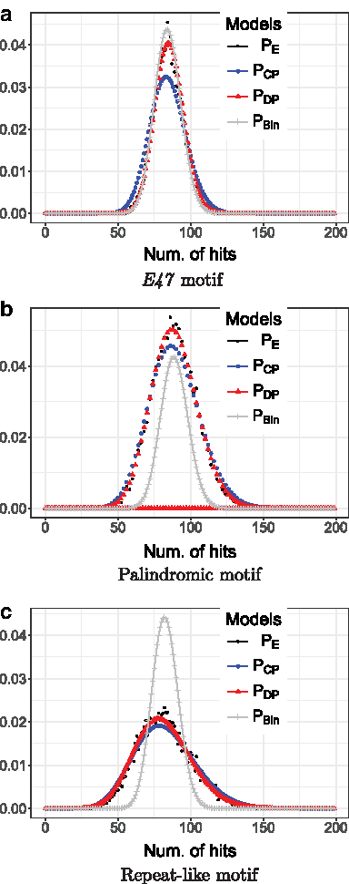
We demonstrate the accuracy of the dynamic programming approach for various parameter settings and a large set of known motifs, including a palindromic motif and a repeat-like motif, in comparison to our earlier compound Poisson model (Kopp and Vingron, 2017) and a binomial model. Generally, we find that the novel dynamic programming approach yields similar or more accurate results compared with the other models, especially when a rather relaxed match score was chosen.
2. Methods
2.1. Motifs, background, motif score, and motif hits
Let \documentclass{aastex}\usepackage{amsbsy}\usepackage{amsfonts}\usepackage{amssymb}\usepackage{bm}\usepackage{mathrsfs}\usepackage{pifont}\usepackage{stmaryrd}\usepackage{textcomp}\usepackage{portland, xspace}\usepackage{amsmath, amsxtra}\usepackage{upgreek}\pagestyle{empty}\DeclareMathSizes{10}{9}{7}{6}\begin{document}
$${ \cal A} = \{ A , C , G , T \} $$
\end{document} denote the alphabet of DNA letters and \documentclass{aastex}\usepackage{amsbsy}\usepackage{amsfonts}\usepackage{amssymb}\usepackage{bm}\usepackage{mathrsfs}\usepackage{pifont}\usepackage{stmaryrd}\usepackage{textcomp}\usepackage{portland, xspace}\usepackage{amsmath, amsxtra}\usepackage{upgreek}\pagestyle{empty}\DeclareMathSizes{10}{9}{7}{6}\begin{document}
$${ \bf{w}} = {w_1}{w_2} \cdots {w_N}$$
\end{document} a sequence of length N from this alphabet. The probability of w is given by a homogeneous order-d Markov model (the background model), whose transition probabilities are denoted by \documentclass{aastex}\usepackage{amsbsy}\usepackage{amsfonts}\usepackage{amssymb}\usepackage{bm}\usepackage{mathrsfs}\usepackage{pifont}\usepackage{stmaryrd}\usepackage{textcomp}\usepackage{portland, xspace}\usepackage{amsmath, amsxtra}\usepackage{upgreek}\pagestyle{empty}\DeclareMathSizes{10}{9}{7}{6}\begin{document}
$$\pi ( {w_{i - d}} \cdots {w_{i - 1}};{w_i} ) = P ( {w_i} \vert {w_{i - 1}} \cdots {w_{i - d}} )$$
\end{document} and whose stationary distribution is denoted by μ. Thus, we have
\documentclass{aastex}\usepackage{amsbsy}\usepackage{amsfonts}\usepackage{amssymb}\usepackage{bm}\usepackage{mathrsfs}\usepackage{pifont}\usepackage{stmaryrd}\usepackage{textcomp}\usepackage{portland, xspace}\usepackage{amsmath, amsxtra}\usepackage{upgreek}\pagestyle{empty}\DeclareMathSizes{10}{9}{7}{6}\begin{document}
\begin{align*}
{P_B} ( { \bf{w}} ) = \mu ( {w_1} \cdots {w_d} ) \prod \limits_{i = d + 1}^N \pi ( {w_{i - d}} \cdots {w_{i - 1}};{w_i} ).
\end{align*}
\end{document}
The transition probabilities \documentclass{aastex}\usepackage{amsbsy}\usepackage{amsfonts}\usepackage{amssymb}\usepackage{bm}\usepackage{mathrsfs}\usepackage{pifont}\usepackage{stmaryrd}\usepackage{textcomp}\usepackage{portland, xspace}\usepackage{amsmath, amsxtra}\usepackage{upgreek}\pagestyle{empty}\DeclareMathSizes{10}{9}{7}{6}\begin{document}
$$\pi ( {a_0} \cdots {a_{d - 1}};{a_d} )$$
\end{document} are estimated via the maximum likelihood procedure described in Reinert et al. (2000):
\documentclass{aastex}\usepackage{amsbsy}\usepackage{amsfonts}\usepackage{amssymb}\usepackage{bm}\usepackage{mathrsfs}\usepackage{pifont}\usepackage{stmaryrd}\usepackage{textcomp}\usepackage{portland, xspace}\usepackage{amsmath, amsxtra}\usepackage{upgreek}\pagestyle{empty}\DeclareMathSizes{10}{9}{7}{6}\begin{document}
\begin{align*}
\hat \pi ( { a_0 } \cdots { a_ { d - 1 } } ; { a_d } ) = { \frac { N ( { a_0 } \cdots { a_ { d - 1 } } , { a_d } ) } { \sum \nolimits_ { { a_d } } { N ( { a_0 } \cdots { a_ { d - 1 } } , { a_d } ) } } } , \tag { 1 }
\end{align*}
\end{document}
with N(a) denoting the count of \documentclass{aastex}\usepackage{amsbsy}\usepackage{amsfonts}\usepackage{amssymb}\usepackage{bm}\usepackage{mathrsfs}\usepackage{pifont}\usepackage{stmaryrd}\usepackage{textcomp}\usepackage{portland, xspace}\usepackage{amsmath, amsxtra}\usepackage{upgreek}\pagestyle{empty}\DeclareMathSizes{10}{9}{7}{6}\begin{document}
$${ \bf{a}} \in {{ \cal A}^{d + 1}}$$
\end{document} in \documentclass{aastex}\usepackage{amsbsy}\usepackage{amsfonts}\usepackage{amssymb}\usepackage{bm}\usepackage{mathrsfs}\usepackage{pifont}\usepackage{stmaryrd}\usepackage{textcomp}\usepackage{portland, xspace}\usepackage{amsmath, amsxtra}\usepackage{upgreek}\pagestyle{empty}\DeclareMathSizes{10}{9}{7}{6}\begin{document}
$${ \bf{w}} \in {{ \cal A}^N}$$
\end{document} and under the additional constraints that each word occurs equally likely on both DNA strands and with reversed nucleotide order (from 5′ to 3′ and 3′ to 5′). These constraints simplify the motif matching statistics when both DNA strands are scanned for motif matches and they are enforced by utilizing the detailed balance condition (Kopp and Vingron, 2017).
We represent the DNA binding affinity by a PFM. A PFM is a \documentclass{aastex}\usepackage{amsbsy}\usepackage{amsfonts}\usepackage{amssymb}\usepackage{bm}\usepackage{mathrsfs}\usepackage{pifont}\usepackage{stmaryrd}\usepackage{textcomp}\usepackage{portland, xspace}\usepackage{amsmath, amsxtra}\usepackage{upgreek}\pagestyle{empty}\DeclareMathSizes{10}{9}{7}{6}\begin{document}
$$\vert { \cal A} \vert \times M$$
\end{document} matrix, where \documentclass{aastex}\usepackage{amsbsy}\usepackage{amsfonts}\usepackage{amssymb}\usepackage{bm}\usepackage{mathrsfs}\usepackage{pifont}\usepackage{stmaryrd}\usepackage{textcomp}\usepackage{portland, xspace}\usepackage{amsmath, amsxtra}\usepackage{upgreek}\pagestyle{empty}\DeclareMathSizes{10}{9}{7}{6}\begin{document}
$$\vert { \cal A} \vert$$
\end{document} denotes the size of the alphabet and M denotes the length of the TF binding site. A PFM contains the elements \documentclass{aastex}\usepackage{amsbsy}\usepackage{amsfonts}\usepackage{amssymb}\usepackage{bm}\usepackage{mathrsfs}\usepackage{pifont}\usepackage{stmaryrd}\usepackage{textcomp}\usepackage{portland, xspace}\usepackage{amsmath, amsxtra}\usepackage{upgreek}\pagestyle{empty}\DeclareMathSizes{10}{9}{7}{6}\begin{document}
$${p_j} ( w )$$
\end{document}, which correspond to the frequency of observing nucleotide w at position j. We shall further assume that all elements of the PFM are strictly positive and its columns are normalized to 1 such that they represent probabilities. Then, the likelihood of a word \documentclass{aastex}\usepackage{amsbsy}\usepackage{amsfonts}\usepackage{amssymb}\usepackage{bm}\usepackage{mathrsfs}\usepackage{pifont}\usepackage{stmaryrd}\usepackage{textcomp}\usepackage{portland, xspace}\usepackage{amsmath, amsxtra}\usepackage{upgreek}\pagestyle{empty}\DeclareMathSizes{10}{9}{7}{6}\begin{document}
$${ \bf{w}} \prime \in {{ \cal A}^M}$$
\end{document} with respect to the PFM is given by
\documentclass{aastex}\usepackage{amsbsy}\usepackage{amsfonts}\usepackage{amssymb}\usepackage{bm}\usepackage{mathrsfs}\usepackage{pifont}\usepackage{stmaryrd}\usepackage{textcomp}\usepackage{portland, xspace}\usepackage{amsmath, amsxtra}\usepackage{upgreek}\pagestyle{empty}\DeclareMathSizes{10}{9}{7}{6}\begin{document}
\begin{align*}
{P_M} ( { \bf{w}} \prime ) = \prod \limits_{j = 1}^M {p_j} ( {w \prime _j} ).
\end{align*}
\end{document}
We adapt the commonly used log-likelihood ratio (Rahmann et al., 2003; Li and Tompa, 2006; Touzet et al., 2007), or motif score, to discriminate likely bound sequences from unbound sequences according to
\documentclass{aastex}\usepackage{amsbsy}\usepackage{amsfonts}\usepackage{amssymb}\usepackage{bm}\usepackage{mathrsfs}\usepackage{pifont}\usepackage{stmaryrd}\usepackage{textcomp}\usepackage{portland, xspace}\usepackage{amsmath, amsxtra}\usepackage{upgreek}\pagestyle{empty}\DeclareMathSizes{10}{9}{7}{6}\begin{document}
\begin{align*}
s ( { \bf { w } } \prime ): = \log \left( { { \frac { { P_M } ( { \bf { w } } \prime ) } { { P_B } ( { \bf { w } } \prime ) } } } \right) , \tag { 2 }
\end{align*}
\end{document}
where \documentclass{aastex}\usepackage{amsbsy}\usepackage{amsfonts}\usepackage{amssymb}\usepackage{bm}\usepackage{mathrsfs}\usepackage{pifont}\usepackage{stmaryrd}\usepackage{textcomp}\usepackage{portland, xspace}\usepackage{amsmath, amsxtra}\usepackage{upgreek}\pagestyle{empty}\DeclareMathSizes{10}{9}{7}{6}\begin{document}
$${ \bf{w}} \prime \in {{ \cal A}^M}$$
\end{document} and assume that \documentclass{aastex}\usepackage{amsbsy}\usepackage{amsfonts}\usepackage{amssymb}\usepackage{bm}\usepackage{mathrsfs}\usepackage{pifont}\usepackage{stmaryrd}\usepackage{textcomp}\usepackage{portland, xspace}\usepackage{amsmath, amsxtra}\usepackage{upgreek}\pagestyle{empty}\DeclareMathSizes{10}{9}{7}{6}\begin{document}
$$d \le M$$
\end{document} for the remainder of this article.
We leverage the motif score to determine motif hits (or putative TFBSs) by utilizing a predetermined score threshold. Position i in a sequence is called a motif hit if \documentclass{aastex}\usepackage{amsbsy}\usepackage{amsfonts}\usepackage{amssymb}\usepackage{bm}\usepackage{mathrsfs}\usepackage{pifont}\usepackage{stmaryrd}\usepackage{textcomp}\usepackage{portland, xspace}\usepackage{amsmath, amsxtra}\usepackage{upgreek}\pagestyle{empty}\DeclareMathSizes{10}{9}{7}{6}\begin{document}
$$s ( {w_i} \ldots {w_{i + M - 1}} )$$
\end{document} is greater or equal to the score threshold. According to Neyman and Pearson (1933), it is reasonable to choose a score threshold \documentclass{aastex}\usepackage{amsbsy}\usepackage{amsfonts}\usepackage{amssymb}\usepackage{bm}\usepackage{mathrsfs}\usepackage{pifont}\usepackage{stmaryrd}\usepackage{textcomp}\usepackage{portland, xspace}\usepackage{amsmath, amsxtra}\usepackage{upgreek}\pagestyle{empty}\DeclareMathSizes{10}{9}{7}{6}\begin{document}
$${t_ \alpha }$$
\end{document}, which is associated with a desired false-positive level α. Hence, motif hits are called with significance level α. To choose \documentclass{aastex}\usepackage{amsbsy}\usepackage{amsfonts}\usepackage{amssymb}\usepackage{bm}\usepackage{mathrsfs}\usepackage{pifont}\usepackage{stmaryrd}\usepackage{textcomp}\usepackage{portland, xspace}\usepackage{amsmath, amsxtra}\usepackage{upgreek}\pagestyle{empty}\DeclareMathSizes{10}{9}{7}{6}\begin{document}
$${t_ \alpha }$$
\end{document}, we determine the distribution of the scores \documentclass{aastex}\usepackage{amsbsy}\usepackage{amsfonts}\usepackage{amssymb}\usepackage{bm}\usepackage{mathrsfs}\usepackage{pifont}\usepackage{stmaryrd}\usepackage{textcomp}\usepackage{portland, xspace}\usepackage{amsmath, amsxtra}\usepackage{upgreek}\pagestyle{empty}\DeclareMathSizes{10}{9}{7}{6}\begin{document}
$${P_B} ( S = s )$$
\end{document} using an efficient algorithm, where we assume the underlying sequence to be generated by an order-d background model starting in the stationary distribution μ as described previously (Kopp and Vingron, 2017). We obtain the score threshold\documentclass{aastex}\usepackage{amsbsy}\usepackage{amsfonts}\usepackage{amssymb}\usepackage{bm}\usepackage{mathrsfs}\usepackage{pifont}\usepackage{stmaryrd}\usepackage{textcomp}\usepackage{portland, xspace}\usepackage{amsmath, amsxtra}\usepackage{upgreek}\pagestyle{empty}\DeclareMathSizes{10}{9}{7}{6}\begin{document}
$${t_ \alpha }$$
\end{document} associated with significance level α from \documentclass{aastex}\usepackage{amsbsy}\usepackage{amsfonts}\usepackage{amssymb}\usepackage{bm}\usepackage{mathrsfs}\usepackage{pifont}\usepackage{stmaryrd}\usepackage{textcomp}\usepackage{portland, xspace}\usepackage{amsmath, amsxtra}\usepackage{upgreek}\pagestyle{empty}\DeclareMathSizes{10}{9}{7}{6}\begin{document}
$${P_B} ( S = s )$$
\end{document} by computing \documentclass{aastex}\usepackage{amsbsy}\usepackage{amsfonts}\usepackage{amssymb}\usepackage{bm}\usepackage{mathrsfs}\usepackage{pifont}\usepackage{stmaryrd}\usepackage{textcomp}\usepackage{portland, xspace}\usepackage{amsmath, amsxtra}\usepackage{upgreek}\pagestyle{empty}\DeclareMathSizes{10}{9}{7}{6}\begin{document}
$${P_B} ( S \ge {t_ \alpha } ) = \alpha$$
\end{document}.
Scanning a DNA sequence for motif matches results in a stochastic process \documentclass{aastex}\usepackage{amsbsy}\usepackage{amsfonts}\usepackage{amssymb}\usepackage{bm}\usepackage{mathrsfs}\usepackage{pifont}\usepackage{stmaryrd}\usepackage{textcomp}\usepackage{portland, xspace}\usepackage{amsmath, amsxtra}\usepackage{upgreek}\pagestyle{empty}\DeclareMathSizes{10}{9}{7}{6}\begin{document}
$${ \{ {Y_i} \} _{1 \le i \le N - M + 1}}$$
\end{document}, where \documentclass{aastex}\usepackage{amsbsy}\usepackage{amsfonts}\usepackage{amssymb}\usepackage{bm}\usepackage{mathrsfs}\usepackage{pifont}\usepackage{stmaryrd}\usepackage{textcomp}\usepackage{portland, xspace}\usepackage{amsmath, amsxtra}\usepackage{upgreek}\pagestyle{empty}\DeclareMathSizes{10}{9}{7}{6}\begin{document}
$${Y_i}: = { \bf{1}} [ s ( {w_i} \cdots {w_{i + M - 1}} ) \ge {t_ \alpha } ]$$
\end{document} denotes an indicator random variable that reflects a TFBS occurrence at position i. In case both DNA strands are scanned for motif matches, an additional set of random variables, denoted by \documentclass{aastex}\usepackage{amsbsy}\usepackage{amsfonts}\usepackage{amssymb}\usepackage{bm}\usepackage{mathrsfs}\usepackage{pifont}\usepackage{stmaryrd}\usepackage{textcomp}\usepackage{portland, xspace}\usepackage{amsmath, amsxtra}\usepackage{upgreek}\pagestyle{empty}\DeclareMathSizes{10}{9}{7}{6}\begin{document}
$${ \{ {Y \prime _i} \} _{1 \le i \le N - M + 1}}$$
\end{document}, reflects the reverse strand matches. The total number of motif matches X emitted on both DNA strands is given by
\documentclass{aastex}\usepackage{amsbsy}\usepackage{amsfonts}\usepackage{amssymb}\usepackage{bm}\usepackage{mathrsfs}\usepackage{pifont}\usepackage{stmaryrd}\usepackage{textcomp}\usepackage{portland, xspace}\usepackage{amsmath, amsxtra}\usepackage{upgreek}\pagestyle{empty}\DeclareMathSizes{10}{9}{7}{6}\begin{document}
\begin{align*}
X = \mathop \sum \limits_{i = 1}^{N - M + 1} {Y_i} + {Y \prime _i}.
\end{align*}
\end{document}
If only one strand is scanned, the contribution of \documentclass{aastex}\usepackage{amsbsy}\usepackage{amsfonts}\usepackage{amssymb}\usepackage{bm}\usepackage{mathrsfs}\usepackage{pifont}\usepackage{stmaryrd}\usepackage{textcomp}\usepackage{portland, xspace}\usepackage{amsmath, amsxtra}\usepackage{upgreek}\pagestyle{empty}\DeclareMathSizes{10}{9}{7}{6}\begin{document}
$${Y \prime _i}$$
\end{document} becomes obsolete.
2.2. Types of matches
Scanning a DNA sequence for binding site matches might result in self-overlapping matches, depending on the structure of the motif, which influences the distribution of the number of motif matches. To account for that, the notion of a clump has been introduced, which refers to one or more motif matches that are mutually overlapping (Reinert et al., 2000).
Within a clump, two distinct types of motif matches are possible: A clump start match and self-overlapping matches. Without loss of generality, we scan for motif matches from left to right. Therefore, a match \documentclass{aastex}\usepackage{amsbsy}\usepackage{amsfonts}\usepackage{amssymb}\usepackage{bm}\usepackage{mathrsfs}\usepackage{pifont}\usepackage{stmaryrd}\usepackage{textcomp}\usepackage{portland, xspace}\usepackage{amsmath, amsxtra}\usepackage{upgreek}\pagestyle{empty}\DeclareMathSizes{10}{9}{7}{6}\begin{document}
$${Y_i} = 1$$
\end{document} at position i starts a clump if it is not overlapped by any previous matches to its left. For example, for a motif of length M = 3, the sequence \documentclass{aastex}\usepackage{amsbsy}\usepackage{amsfonts}\usepackage{amssymb}\usepackage{bm}\usepackage{mathrsfs}\usepackage{pifont}\usepackage{stmaryrd}\usepackage{textcomp}\usepackage{portland, xspace}\usepackage{amsmath, amsxtra}\usepackage{upgreek}\pagestyle{empty}\DeclareMathSizes{10}{9}{7}{6}\begin{document}
$${Y_1} = 0 , {Y_2} = 0 , {Y_3} = 1$$
\end{document} constitutes a clump start at position 3. Otherwise, we observe a self-overlapping match.
2.2.1. Motif matches when scanning a single strand
The probability of observing a clump start is denoted by
\documentclass{aastex}\usepackage{amsbsy}\usepackage{amsfonts}\usepackage{amssymb}\usepackage{bm}\usepackage{mathrsfs}\usepackage{pifont}\usepackage{stmaryrd}\usepackage{textcomp}\usepackage{portland, xspace}\usepackage{amsmath, amsxtra}\usepackage{upgreek}\pagestyle{empty}\DeclareMathSizes{10}{9}{7}{6}\begin{document}
\begin{align*}
\tau: = P ( {Y_i} = 1 \vert {Y_{i - 1}} = 0 , \cdots , {Y_{i - M + 1}} = 0 ). \tag{3}
\end{align*}
\end{document}
The computation of the clump start probability shall be deferred to Section 2.3. We define the probability of a self-overlapping match by
\documentclass{aastex}\usepackage{amsbsy}\usepackage{amsfonts}\usepackage{amssymb}\usepackage{bm}\usepackage{mathrsfs}\usepackage{pifont}\usepackage{stmaryrd}\usepackage{textcomp}\usepackage{portland, xspace}\usepackage{amsmath, amsxtra}\usepackage{upgreek}\pagestyle{empty}\DeclareMathSizes{10}{9}{7}{6}\begin{document}
\begin{align*}
{ \beta _k}: = P ( {Y_k} = 1 , {Y_{k - 1}} = 0 , \cdots {Y_1} = 0 \vert {Y_0} = 1 ) \tag{4}
\end{align*}
\end{document}
for \documentclass{aastex}\usepackage{amsbsy}\usepackage{amsfonts}\usepackage{amssymb}\usepackage{bm}\usepackage{mathrsfs}\usepackage{pifont}\usepackage{stmaryrd}\usepackage{textcomp}\usepackage{portland, xspace}\usepackage{amsmath, amsxtra}\usepackage{upgreek}\pagestyle{empty}\DeclareMathSizes{10}{9}{7}{6}\begin{document}
$$k \in \{ 1 , \cdots M - 1 \} $$
\end{document}, which we efficiently approximate using our earlier approach (Kopp and Vingron, 2017).
2.2.2. Motif matches when scanning both DNA strands
In many applications, we do not know in advance on which DNA strand a TFBS might occur, which is solved by simply scanning both strands. This in turn also creates a coupling between matches on both strands that needs to be addressed. In the following, without loss of generality, we consider the ordering of events: \documentclass{aastex}\usepackage{amsbsy}\usepackage{amsfonts}\usepackage{amssymb}\usepackage{bm}\usepackage{mathrsfs}\usepackage{pifont}\usepackage{stmaryrd}\usepackage{textcomp}\usepackage{portland, xspace}\usepackage{amsmath, amsxtra}\usepackage{upgreek}\pagestyle{empty}\DeclareMathSizes{10}{9}{7}{6}\begin{document}
$${Y_1}{Y \prime _1} \,{Y_2} \,{Y \prime _2} \,{Y_3} \,{Y \prime _3} \cdots$$
\end{document}. That is, we scan the sequence from left to right, and a forward strand event Yi precedes the corresponding reverse strand event \documentclass{aastex}\usepackage{amsbsy}\usepackage{amsfonts}\usepackage{amssymb}\usepackage{bm}\usepackage{mathrsfs}\usepackage{pifont}\usepackage{stmaryrd}\usepackage{textcomp}\usepackage{portland, xspace}\usepackage{amsmath, amsxtra}\usepackage{upgreek}\pagestyle{empty}\DeclareMathSizes{10}{9}{7}{6}\begin{document}
$${Y \prime _i}$$
\end{document} at position i.
A clump starts on the forward strand if matches at the \documentclass{aastex}\usepackage{amsbsy}\usepackage{amsfonts}\usepackage{amssymb}\usepackage{bm}\usepackage{mathrsfs}\usepackage{pifont}\usepackage{stmaryrd}\usepackage{textcomp}\usepackage{portland, xspace}\usepackage{amsmath, amsxtra}\usepackage{upgreek}\pagestyle{empty}\DeclareMathSizes{10}{9}{7}{6}\begin{document}
$$M - 1$$
\end{document} previous positions (on both strands) are absent. Its probability is defined by
\documentclass{aastex}\usepackage{amsbsy}\usepackage{amsfonts}\usepackage{amssymb}\usepackage{bm}\usepackage{mathrsfs}\usepackage{pifont}\usepackage{stmaryrd}\usepackage{textcomp}\usepackage{portland, xspace}\usepackage{amsmath, amsxtra}\usepackage{upgreek}\pagestyle{empty}\DeclareMathSizes{10}{9}{7}{6}\begin{document}
\begin{align*}
\tau: = P ( {Y_i} = 1 \vert \{ {Y_{i - m}} = 0 , {Y \prime _{i - m}}{ = 0 \} _{i - M < m < i}} ). \tag{5}
\end{align*}
\end{document}
Likewise, a clump starts on the reverse strand \documentclass{aastex}\usepackage{amsbsy}\usepackage{amsfonts}\usepackage{amssymb}\usepackage{bm}\usepackage{mathrsfs}\usepackage{pifont}\usepackage{stmaryrd}\usepackage{textcomp}\usepackage{portland, xspace}\usepackage{amsmath, amsxtra}\usepackage{upgreek}\pagestyle{empty}\DeclareMathSizes{10}{9}{7}{6}\begin{document}
$${Y \prime _i} = 1$$
\end{document} if additionally \documentclass{aastex}\usepackage{amsbsy}\usepackage{amsfonts}\usepackage{amssymb}\usepackage{bm}\usepackage{mathrsfs}\usepackage{pifont}\usepackage{stmaryrd}\usepackage{textcomp}\usepackage{portland, xspace}\usepackage{amsmath, amsxtra}\usepackage{upgreek}\pagestyle{empty}\DeclareMathSizes{10}{9}{7}{6}\begin{document}
$${Y_i} = 0$$
\end{document}, in which case the probability is given by
\documentclass{aastex}\usepackage{amsbsy}\usepackage{amsfonts}\usepackage{amssymb}\usepackage{bm}\usepackage{mathrsfs}\usepackage{pifont}\usepackage{stmaryrd}\usepackage{textcomp}\usepackage{portland, xspace}\usepackage{amsmath, amsxtra}\usepackage{upgreek}\pagestyle{empty}\DeclareMathSizes{10}{9}{7}{6}\begin{document}
\begin{align*}
\tau \prime: = P ( {Y \prime _i} = 1 , {Y_i} = 0 \vert \{ {Y_{i - m}} = 0 , {Y \prime _{i - m}}{ = 0 \} _{i - M < m < i}} ). \tag{6}
\end{align*}
\end{document}
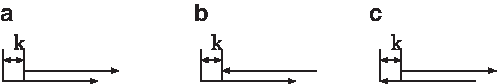
When scanning both DNA strands, overlapping motif matches might occur in three different configurations: (1) Hits might overlap on the same strand, (2) a forward strand hit \documentclass{aastex}\usepackage{amsbsy}\usepackage{amsfonts}\usepackage{amssymb}\usepackage{bm}\usepackage{mathrsfs}\usepackage{pifont}\usepackage{stmaryrd}\usepackage{textcomp}\usepackage{portland, xspace}\usepackage{amsmath, amsxtra}\usepackage{upgreek}\pagestyle{empty}\DeclareMathSizes{10}{9}{7}{6}\begin{document}
$${Y_0} = 1$$
\end{document} precedes a reverse strand hit \documentclass{aastex}\usepackage{amsbsy}\usepackage{amsfonts}\usepackage{amssymb}\usepackage{bm}\usepackage{mathrsfs}\usepackage{pifont}\usepackage{stmaryrd}\usepackage{textcomp}\usepackage{portland, xspace}\usepackage{amsmath, amsxtra}\usepackage{upgreek}\pagestyle{empty}\DeclareMathSizes{10}{9}{7}{6}\begin{document}
$${Y \prime _k} = 1$$
\end{document} for \documentclass{aastex}\usepackage{amsbsy}\usepackage{amsfonts}\usepackage{amssymb}\usepackage{bm}\usepackage{mathrsfs}\usepackage{pifont}\usepackage{stmaryrd}\usepackage{textcomp}\usepackage{portland, xspace}\usepackage{amsmath, amsxtra}\usepackage{upgreek}\pagestyle{empty}\DeclareMathSizes{10}{9}{7}{6}\begin{document}
$$0 \le k < M$$
\end{document}, and (3) a reverse strand hit \documentclass{aastex}\usepackage{amsbsy}\usepackage{amsfonts}\usepackage{amssymb}\usepackage{bm}\usepackage{mathrsfs}\usepackage{pifont}\usepackage{stmaryrd}\usepackage{textcomp}\usepackage{portland, xspace}\usepackage{amsmath, amsxtra}\usepackage{upgreek}\pagestyle{empty}\DeclareMathSizes{10}{9}{7}{6}\begin{document}
$${Y \prime _0} = 1$$
\end{document} precedes a forward strand hit \documentclass{aastex}\usepackage{amsbsy}\usepackage{amsfonts}\usepackage{amssymb}\usepackage{bm}\usepackage{mathrsfs}\usepackage{pifont}\usepackage{stmaryrd}\usepackage{textcomp}\usepackage{portland, xspace}\usepackage{amsmath, amsxtra}\usepackage{upgreek}\pagestyle{empty}\DeclareMathSizes{10}{9}{7}{6}\begin{document}
$${Y_k} = 1$$
\end{document} for \documentclass{aastex}\usepackage{amsbsy}\usepackage{amsfonts}\usepackage{amssymb}\usepackage{bm}\usepackage{mathrsfs}\usepackage{pifont}\usepackage{stmaryrd}\usepackage{textcomp}\usepackage{portland, xspace}\usepackage{amsmath, amsxtra}\usepackage{upgreek}\pagestyle{empty}\DeclareMathSizes{10}{9}{7}{6}\begin{document}
$$0 < k < M$$
\end{document}, where k denotes the shift between the positions (Fig. 1).
Three types of overlapping hit with a shift of k between the motif starts. (a), (b), and (c) correspond to matches on the same strand, a forward strand match followed by a reverse strand match and a reverse strand match followed by a forward strand match, respectively. The arrows pointing to the right and left represent the (5′→3′) and (3′←5′) directions of the DNA, respectively.
The associated probabilities with the overlapping match configurations are defined by
\documentclass{aastex}\usepackage{amsbsy}\usepackage{amsfonts}\usepackage{amssymb}\usepackage{bm}\usepackage{mathrsfs}\usepackage{pifont}\usepackage{stmaryrd}\usepackage{textcomp}\usepackage{portland, xspace}\usepackage{amsmath, amsxtra}\usepackage{upgreek}\pagestyle{empty}\DeclareMathSizes{10}{9}{7}{6}\begin{document}
\begin{align*}
{ \beta _k}: = P ( {Y_k} = 1 , \{ {Y_j} = 0 , {Y \prime { _j}}{ = 0 \} _{1 \le j < k}} , {Y \prime { _0}} = 0 \vert {Y_0} = 1 ) \tag{7}
\end{align*}
\end{document}
We approximate them by using the procedure discussed in Kopp and Vingron (2017).
2.3. A Markov model for generating motif matches
In this section, we introduce a Markov model that resembles the process of generating motif matches as one DNA strand is scanned for match occurrences. We shall exploit this model later to determine the clump start probability, which constitutes an important prerequisite for Section 2.4.
2.3.1. Model states, state transitions, and transition probabilities
Before establishing the Markov model states, two independence assumptions are required: First, for \documentclass{aastex}\usepackage{amsbsy}\usepackage{amsfonts}\usepackage{amssymb}\usepackage{bm}\usepackage{mathrsfs}\usepackage{pifont}\usepackage{stmaryrd}\usepackage{textcomp}\usepackage{portland, xspace}\usepackage{amsmath, amsxtra}\usepackage{upgreek}\pagestyle{empty}\DeclareMathSizes{10}{9}{7}{6}\begin{document}
$$i + M - 1 < j$$
\end{document}, the events Yi and Yj are assumed to be statistically independent because they are nonoverlapping. Second, a motif match \documentclass{aastex}\usepackage{amsbsy}\usepackage{amsfonts}\usepackage{amssymb}\usepackage{bm}\usepackage{mathrsfs}\usepackage{pifont}\usepackage{stmaryrd}\usepackage{textcomp}\usepackage{portland, xspace}\usepackage{amsmath, amsxtra}\usepackage{upgreek}\pagestyle{empty}\DeclareMathSizes{10}{9}{7}{6}\begin{document}
$${Y_i} = 1$$
\end{document} at position i renders the events upstream and downstream independent, for example, \documentclass{aastex}\usepackage{amsbsy}\usepackage{amsfonts}\usepackage{amssymb}\usepackage{bm}\usepackage{mathrsfs}\usepackage{pifont}\usepackage{stmaryrd}\usepackage{textcomp}\usepackage{portland, xspace}\usepackage{amsmath, amsxtra}\usepackage{upgreek}\pagestyle{empty}\DeclareMathSizes{10}{9}{7}{6}\begin{document}
$${Y_{i - 1}}$$
\end{document} is independent of \documentclass{aastex}\usepackage{amsbsy}\usepackage{amsfonts}\usepackage{amssymb}\usepackage{bm}\usepackage{mathrsfs}\usepackage{pifont}\usepackage{stmaryrd}\usepackage{textcomp}\usepackage{portland, xspace}\usepackage{amsmath, amsxtra}\usepackage{upgreek}\pagestyle{empty}\DeclareMathSizes{10}{9}{7}{6}\begin{document}
$${Y_{i + 1}}$$
\end{document} given \documentclass{aastex}\usepackage{amsbsy}\usepackage{amsfonts}\usepackage{amssymb}\usepackage{bm}\usepackage{mathrsfs}\usepackage{pifont}\usepackage{stmaryrd}\usepackage{textcomp}\usepackage{portland, xspace}\usepackage{amsmath, amsxtra}\usepackage{upgreek}\pagestyle{empty}\DeclareMathSizes{10}{9}{7}{6}\begin{document}
$${Y_i} = 1$$
\end{document}. We justify them in Section 5.
Next, we define the Markov model and use it to express the realizations of \documentclass{aastex}\usepackage{amsbsy}\usepackage{amsfonts}\usepackage{amssymb}\usepackage{bm}\usepackage{mathrsfs}\usepackage{pifont}\usepackage{stmaryrd}\usepackage{textcomp}\usepackage{portland, xspace}\usepackage{amsmath, amsxtra}\usepackage{upgreek}\pagestyle{empty}\DeclareMathSizes{10}{9}{7}{6}\begin{document}
$${Y_1}{Y_2}{Y_3} \cdots$$
\end{document} in terms of the states and state transition. We shall use the Markov model to analyze the stationary distribution of the model, which allows us to evaluate the unknown probability of a clump start match τ.
where “•” represents any outcome (zero or one) at the respective position. As the motif is shifted along the sequence, the Markov chain switches from one state to another, determined by the match pattern of the motif at a position. State h represents a motif match at a current position i regardless of the previous events. nk denotes a memory state that indicates that the last match occurred k positions upstream of the current position and n denotes the absence of motif matches for \documentclass{aastex}\usepackage{amsbsy}\usepackage{amsfonts}\usepackage{amssymb}\usepackage{bm}\usepackage{mathrsfs}\usepackage{pifont}\usepackage{stmaryrd}\usepackage{textcomp}\usepackage{portland, xspace}\usepackage{amsmath, amsxtra}\usepackage{upgreek}\pagestyle{empty}\DeclareMathSizes{10}{9}{7}{6}\begin{document}
$$M - 1$$
\end{document} consecutive position (including the current position).
Traversing the sequence \documentclass{aastex}\usepackage{amsbsy}\usepackage{amsfonts}\usepackage{amssymb}\usepackage{bm}\usepackage{mathrsfs}\usepackage{pifont}\usepackage{stmaryrd}\usepackage{textcomp}\usepackage{portland, xspace}\usepackage{amsmath, amsxtra}\usepackage{upgreek}\pagestyle{empty}\DeclareMathSizes{10}{9}{7}{6}\begin{document}
$${Y_1}{Y_2}{Y_3} \cdots$$
\end{document} in an ordered manner imposes a restriction on the possible state transitions (Fig. 2). For example, the transition \documentclass{aastex}\usepackage{amsbsy}\usepackage{amsfonts}\usepackage{amssymb}\usepackage{bm}\usepackage{mathrsfs}\usepackage{pifont}\usepackage{stmaryrd}\usepackage{textcomp}\usepackage{portland, xspace}\usepackage{amsmath, amsxtra}\usepackage{upgreek}\pagestyle{empty}\DeclareMathSizes{10}{9}{7}{6}\begin{document}
$$( {Z_i} = {n_2} ) \to ( {Z_{i + 1}} = {n_1} )$$
\end{document} is not viable, whereas \documentclass{aastex}\usepackage{amsbsy}\usepackage{amsfonts}\usepackage{amssymb}\usepackage{bm}\usepackage{mathrsfs}\usepackage{pifont}\usepackage{stmaryrd}\usepackage{textcomp}\usepackage{portland, xspace}\usepackage{amsmath, amsxtra}\usepackage{upgreek}\pagestyle{empty}\DeclareMathSizes{10}{9}{7}{6}\begin{document}
$$( {Z_i} = n ) \to ( {Z_{i + 1}} = h )$$
\end{document} is. This in turn results in an M × M transition matrix:
Illustration of the Markov model. The nodes denote the states of the model using a TF motif of length M = 5. Arrows indicate viable state transitions, which may (or may not) be associated with a positive transition probabilities. Underneath each node, the associated pattern in \documentclass{aastex}\usepackage{amsbsy}\usepackage{amsfonts}\usepackage{amssymb}\usepackage{bm}\usepackage{mathrsfs}\usepackage{pifont}\usepackage{stmaryrd}\usepackage{textcomp}\usepackage{portland, xspace}\usepackage{amsmath, amsxtra}\usepackage{upgreek}\pagestyle{empty}\DeclareMathSizes{10}{9}{7}{6}\begin{document}
$${Y_1}{Y_2} \cdots$$
\end{document} is depicted, where the black and white boxes denote the outcomes one and zero and the bullet represents any outcome (zero or one) that are described by the Correspondences [Equation (11)]. TF, transcription factor.
whose individual transition probabilities are derived from Equations (3) and (4) as
\documentclass{aastex}\usepackage{amsbsy}\usepackage{amsfonts}\usepackage{amssymb}\usepackage{bm}\usepackage{mathrsfs}\usepackage{pifont}\usepackage{stmaryrd}\usepackage{textcomp}\usepackage{portland, xspace}\usepackage{amsmath, amsxtra}\usepackage{upgreek}\pagestyle{empty}\DeclareMathSizes{10}{9}{7}{6}\begin{document}
\begin{align*}
P ( n \to n ): = 1 - \tau \tag{13}
\end{align*}
\end{document}\documentclass{aastex}\usepackage{amsbsy}\usepackage{amsfonts}\usepackage{amssymb}\usepackage{bm}\usepackage{mathrsfs}\usepackage{pifont}\usepackage{stmaryrd}\usepackage{textcomp}\usepackage{portland, xspace}\usepackage{amsmath, amsxtra}\usepackage{upgreek}\pagestyle{empty}\DeclareMathSizes{10}{9}{7}{6}\begin{document}
\begin{align*}
P ( n \to h ): = \tau \tag{14}
\end{align*}
\end{document}\documentclass{aastex}\usepackage{amsbsy}\usepackage{amsfonts}\usepackage{amssymb}\usepackage{bm}\usepackage{mathrsfs}\usepackage{pifont}\usepackage{stmaryrd}\usepackage{textcomp}\usepackage{portland, xspace}\usepackage{amsmath, amsxtra}\usepackage{upgreek}\pagestyle{empty}\DeclareMathSizes{10}{9}{7}{6}\begin{document}
\begin{align*}
P ( h \to h ): = { \beta _1} \tag{15}
\end{align*}
\end{document}\documentclass{aastex}\usepackage{amsbsy}\usepackage{amsfonts}\usepackage{amssymb}\usepackage{bm}\usepackage{mathrsfs}\usepackage{pifont}\usepackage{stmaryrd}\usepackage{textcomp}\usepackage{portland, xspace}\usepackage{amsmath, amsxtra}\usepackage{upgreek}\pagestyle{empty}\DeclareMathSizes{10}{9}{7}{6}\begin{document}
\begin{align*}
P ( h \to {n_1} ): = 1 - { \beta _1} \tag{16}
\end{align*}
\end{document}\documentclass{aastex}\usepackage{amsbsy}\usepackage{amsfonts}\usepackage{amssymb}\usepackage{bm}\usepackage{mathrsfs}\usepackage{pifont}\usepackage{stmaryrd}\usepackage{textcomp}\usepackage{portland, xspace}\usepackage{amsmath, amsxtra}\usepackage{upgreek}\pagestyle{empty}\DeclareMathSizes{10}{9}{7}{6}\begin{document}
\begin{align*}
P ( {n_k} \to h ): = P ( {Y_0} = 1 \vert {Y_{ - 1}} = 0 , \cdots , {Y_{ - k + 1}} = 0 , {Y_{ - k}} = 1 )
\end{align*}
\end{document}\documentclass{aastex}\usepackage{amsbsy}\usepackage{amsfonts}\usepackage{amssymb}\usepackage{bm}\usepackage{mathrsfs}\usepackage{pifont}\usepackage{stmaryrd}\usepackage{textcomp}\usepackage{portland, xspace}\usepackage{amsmath, amsxtra}\usepackage{upgreek}\pagestyle{empty}\DeclareMathSizes{10}{9}{7}{6}\begin{document}
\begin{align*}
= { \frac { P ( { Y_k } = 1 , { Y_ { k - 1 } } = 0 , \cdots , { Y_1 } = 0 \vert { Y_0 } = 1 ) } { P ( { Y_ { k - 1 } } = 0 , \cdots , { Y_1 } = 0 \vert { Y_0 } = 1 ) } }
\end{align*}
\end{document}\documentclass{aastex}\usepackage{amsbsy}\usepackage{amsfonts}\usepackage{amssymb}\usepackage{bm}\usepackage{mathrsfs}\usepackage{pifont}\usepackage{stmaryrd}\usepackage{textcomp}\usepackage{portland, xspace}\usepackage{amsmath, amsxtra}\usepackage{upgreek}\pagestyle{empty}\DeclareMathSizes{10}{9}{7}{6}\begin{document}
\begin{align*}
= { \frac { { \beta _k } } { 1 - \mathop \sum \limits_ { i = 1 } ^ { k - 1 } { \beta _i } } } \quad \quad { \rm { for } } \;1 \le k \le M - 2 \tag { 17 }
\end{align*}
\end{document}\documentclass{aastex}\usepackage{amsbsy}\usepackage{amsfonts}\usepackage{amssymb}\usepackage{bm}\usepackage{mathrsfs}\usepackage{pifont}\usepackage{stmaryrd}\usepackage{textcomp}\usepackage{portland, xspace}\usepackage{amsmath, amsxtra}\usepackage{upgreek}\pagestyle{empty}\DeclareMathSizes{10}{9}{7}{6}\begin{document}
\begin{align*}
P ( {n_k} \to {n_{k + 1}} ): = 1 - P ( {n_k} \to h ) \quad \quad { \rm{for}} \;1 \le k < M - 2 \tag{18}
\end{align*}
\end{document}\documentclass{aastex}\usepackage{amsbsy}\usepackage{amsfonts}\usepackage{amssymb}\usepackage{bm}\usepackage{mathrsfs}\usepackage{pifont}\usepackage{stmaryrd}\usepackage{textcomp}\usepackage{portland, xspace}\usepackage{amsmath, amsxtra}\usepackage{upgreek}\pagestyle{empty}\DeclareMathSizes{10}{9}{7}{6}\begin{document}
\begin{align*}
P ( {n_{M - 2}} \to n ): = 1 - P ( {n_{M - 2}} \to h ). \tag{19}
\end{align*}
\end{document}
2.3.2. Computing the clump start probability τ
In the previous section, we have established the states and state transitions for the Markov model. We expressed the transition probabilities solely based on τ and \documentclass{aastex}\usepackage{amsbsy}\usepackage{amsfonts}\usepackage{amssymb}\usepackage{bm}\usepackage{mathrsfs}\usepackage{pifont}\usepackage{stmaryrd}\usepackage{textcomp}\usepackage{portland, xspace}\usepackage{amsmath, amsxtra}\usepackage{upgreek}\pagestyle{empty}\DeclareMathSizes{10}{9}{7}{6}\begin{document}
$${ \{ { \beta _k} \} _{1 \le k \le M - 1}}$$
\end{document}. While \documentclass{aastex}\usepackage{amsbsy}\usepackage{amsfonts}\usepackage{amssymb}\usepackage{bm}\usepackage{mathrsfs}\usepackage{pifont}\usepackage{stmaryrd}\usepackage{textcomp}\usepackage{portland, xspace}\usepackage{amsmath, amsxtra}\usepackage{upgreek}\pagestyle{empty}\DeclareMathSizes{10}{9}{7}{6}\begin{document}
$${ \{ { \beta _k} \} _{1 \le k \le M - 1}}$$
\end{document} can be efficiently approximated, the computation of τ remains to be discussed.
Recall that due to the choice of the score threshold \documentclass{aastex}\usepackage{amsbsy}\usepackage{amsfonts}\usepackage{amssymb}\usepackage{bm}\usepackage{mathrsfs}\usepackage{pifont}\usepackage{stmaryrd}\usepackage{textcomp}\usepackage{portland, xspace}\usepackage{amsmath, amsxtra}\usepackage{upgreek}\pagestyle{empty}\DeclareMathSizes{10}{9}{7}{6}\begin{document}
$${t_ \alpha }$$
\end{document}, motif matches occur with probability \documentclass{aastex}\usepackage{amsbsy}\usepackage{amsfonts}\usepackage{amssymb}\usepackage{bm}\usepackage{mathrsfs}\usepackage{pifont}\usepackage{stmaryrd}\usepackage{textcomp}\usepackage{portland, xspace}\usepackage{amsmath, amsxtra}\usepackage{upgreek}\pagestyle{empty}\DeclareMathSizes{10}{9}{7}{6}\begin{document}
$$P ( Y = 1 ) = \alpha$$
\end{document}. This implies that the stationary distribution of the Markov model should visit the state Z = h also with probability \documentclass{aastex}\usepackage{amsbsy}\usepackage{amsfonts}\usepackage{amssymb}\usepackage{bm}\usepackage{mathrsfs}\usepackage{pifont}\usepackage{stmaryrd}\usepackage{textcomp}\usepackage{portland, xspace}\usepackage{amsmath, amsxtra}\usepackage{upgreek}\pagestyle{empty}\DeclareMathSizes{10}{9}{7}{6}\begin{document}
$$\mu ( Z = h ) = \alpha$$
\end{document}, where μ denotes the stationary probability. Thus, we introduce an optimization procedure whose objective is to establish \documentclass{aastex}\usepackage{amsbsy}\usepackage{amsfonts}\usepackage{amssymb}\usepackage{bm}\usepackage{mathrsfs}\usepackage{pifont}\usepackage{stmaryrd}\usepackage{textcomp}\usepackage{portland, xspace}\usepackage{amsmath, amsxtra}\usepackage{upgreek}\pagestyle{empty}\DeclareMathSizes{10}{9}{7}{6}\begin{document}
$$\mu ( h; \tau ) = \alpha$$
\end{document} with respect to the unknown parameter τ. We utilize the objective function:
\documentclass{aastex}\usepackage{amsbsy}\usepackage{amsfonts}\usepackage{amssymb}\usepackage{bm}\usepackage{mathrsfs}\usepackage{pifont}\usepackage{stmaryrd}\usepackage{textcomp}\usepackage{portland, xspace}\usepackage{amsmath, amsxtra}\usepackage{upgreek}\pagestyle{empty}\DeclareMathSizes{10}{9}{7}{6}\begin{document}
\begin{align*}
f ( \mu ( \tau ) ): = - \alpha \log ( \mu ( h; \tau ) ) - ( 1 - \alpha ) \log ( 1 - \mu ( h; \tau ) ) , \tag{20}
\end{align*}
\end{document}
which has a unique minimum at \documentclass{aastex}\usepackage{amsbsy}\usepackage{amsfonts}\usepackage{amssymb}\usepackage{bm}\usepackage{mathrsfs}\usepackage{pifont}\usepackage{stmaryrd}\usepackage{textcomp}\usepackage{portland, xspace}\usepackage{amsmath, amsxtra}\usepackage{upgreek}\pagestyle{empty}\DeclareMathSizes{10}{9}{7}{6}\begin{document}
$$\mu ( h; \tau ) = \alpha$$
\end{document} as can be verified by studying \documentclass{aastex}\usepackage{amsbsy}\usepackage{amsfonts}\usepackage{amssymb}\usepackage{bm}\usepackage{mathrsfs}\usepackage{pifont}\usepackage{stmaryrd}\usepackage{textcomp}\usepackage{portland, xspace}\usepackage{amsmath, amsxtra}\usepackage{upgreek}\pagestyle{empty}\DeclareMathSizes{10}{9}{7}{6}\begin{document}
$$df ( \mu ) / d \mu = 0$$
\end{document}. This function is motivated by the cross-entropy error, which is widely used to fit supervised statistical classifiers, for example, the logistic regression model (Bishop, 2006). While the objective \documentclass{aastex}\usepackage{amsbsy}\usepackage{amsfonts}\usepackage{amssymb}\usepackage{bm}\usepackage{mathrsfs}\usepackage{pifont}\usepackage{stmaryrd}\usepackage{textcomp}\usepackage{portland, xspace}\usepackage{amsmath, amsxtra}\usepackage{upgreek}\pagestyle{empty}\DeclareMathSizes{10}{9}{7}{6}\begin{document}
$${ ( \mu ( h; \tau ) - \alpha ) ^2}$$
\end{document} would be another (perhaps more intuitive) possibility, it may result in numerical issues due to the fact that α is usually rather small. In contrast, the chosen objective function [Equation (20)] is slightly better behaved in this respect. Furthermore, other objective functions may be envisioned as well, so long as they have a minimum at \documentclass{aastex}\usepackage{amsbsy}\usepackage{amsfonts}\usepackage{amssymb}\usepackage{bm}\usepackage{mathrsfs}\usepackage{pifont}\usepackage{stmaryrd}\usepackage{textcomp}\usepackage{portland, xspace}\usepackage{amsmath, amsxtra}\usepackage{upgreek}\pagestyle{empty}\DeclareMathSizes{10}{9}{7}{6}\begin{document}
$$\mu ( h; \tau ) = \alpha$$
\end{document}. But since we have not noticed any numerical issues with the current choice (as by the experiments presented in this work), we believe that the current objective works well in practice.
We minimize Equation (20) iteratively starting from \documentclass{aastex}\usepackage{amsbsy}\usepackage{amsfonts}\usepackage{amssymb}\usepackage{bm}\usepackage{mathrsfs}\usepackage{pifont}\usepackage{stmaryrd}\usepackage{textcomp}\usepackage{portland, xspace}\usepackage{amsmath, amsxtra}\usepackage{upgreek}\pagestyle{empty}\DeclareMathSizes{10}{9}{7}{6}\begin{document}
$${ \tau _0} = \alpha$$
\end{document} using conjugate gradients. In each iteration, the stationary distribution of the Markov model is computed with respect to the current τ using the power method (Karlin and Taylor, 1981).
2.4. Computing the distribution of the number of matches
In this section, we develop an algorithm for computing the distribution of the number of motif matches based on the previously determined overlapping match probabilities \documentclass{aastex}\usepackage{amsbsy}\usepackage{amsfonts}\usepackage{amssymb}\usepackage{bm}\usepackage{mathrsfs}\usepackage{pifont}\usepackage{stmaryrd}\usepackage{textcomp}\usepackage{portland, xspace}\usepackage{amsmath, amsxtra}\usepackage{upgreek}\pagestyle{empty}\DeclareMathSizes{10}{9}{7}{6}\begin{document}
$${ \{ { \beta _i} \} _{1 \le i < M}}$$
\end{document} and the clump start probability τ. The algorithm was inspired by Liu and Lawrence (1999), which allows to efficiently sum the probabilities of all possible permutations of placing X motif matches in a sequence of fixed length N via dynamic programming. For example, to compute the probability of placing two matches in \documentclass{aastex}\usepackage{amsbsy}\usepackage{amsfonts}\usepackage{amssymb}\usepackage{bm}\usepackage{mathrsfs}\usepackage{pifont}\usepackage{stmaryrd}\usepackage{textcomp}\usepackage{portland, xspace}\usepackage{amsmath, amsxtra}\usepackage{upgreek}\pagestyle{empty}\DeclareMathSizes{10}{9}{7}{6}\begin{document}
$${Y_1}..{Y_3}$$
\end{document}, we would have to determine \documentclass{aastex}\usepackage{amsbsy}\usepackage{amsfonts}\usepackage{amssymb}\usepackage{bm}\usepackage{mathrsfs}\usepackage{pifont}\usepackage{stmaryrd}\usepackage{textcomp}\usepackage{portland, xspace}\usepackage{amsmath, amsxtra}\usepackage{upgreek}\pagestyle{empty}\DeclareMathSizes{10}{9}{7}{6}\begin{document}
$$P ( {Y_1}..{Y_3} = 110 ) + P ( {Y_1}..{Y_3} = 101 ) + P ( {Y_1}..{Y_3} = 011 )$$
\end{document}. In the general case, this amounts to summing over \documentclass{aastex}\usepackage{amsbsy}\usepackage{amsfonts}\usepackage{amssymb}\usepackage{bm}\usepackage{mathrsfs}\usepackage{pifont}\usepackage{stmaryrd}\usepackage{textcomp}\usepackage{portland, xspace}\usepackage{amsmath, amsxtra}\usepackage{upgreek}\pagestyle{empty}\DeclareMathSizes{10}{9}{7}{6}\begin{document}
$$( _x^N )$$
\end{document} individual permutations. While dynamic programming has been proposed for studying word-pattern-based motifs (Zhang et al., 2007), we are not aware of a comparable approach for studying PFM-based motifs directly.
We start by discussing the case where overlapping motif matches are ignored. We denote the indices associated with the events \documentclass{aastex}\usepackage{amsbsy}\usepackage{amsfonts}\usepackage{amssymb}\usepackage{bm}\usepackage{mathrsfs}\usepackage{pifont}\usepackage{stmaryrd}\usepackage{textcomp}\usepackage{portland, xspace}\usepackage{amsmath, amsxtra}\usepackage{upgreek}\pagestyle{empty}\DeclareMathSizes{10}{9}{7}{6}\begin{document}
$${Y_1} \cdots {Y_i}$$
\end{document} by \documentclass{aastex}\usepackage{amsbsy}\usepackage{amsfonts}\usepackage{amssymb}\usepackage{bm}\usepackage{mathrsfs}\usepackage{pifont}\usepackage{stmaryrd}\usepackage{textcomp}\usepackage{portland, xspace}\usepackage{amsmath, amsxtra}\usepackage{upgreek}\pagestyle{empty}\DeclareMathSizes{10}{9}{7}{6}\begin{document}
$$[ 1:i ]$$
\end{document}. The number of motif matches in that segment is denoted by \documentclass{aastex}\usepackage{amsbsy}\usepackage{amsfonts}\usepackage{amssymb}\usepackage{bm}\usepackage{mathrsfs}\usepackage{pifont}\usepackage{stmaryrd}\usepackage{textcomp}\usepackage{portland, xspace}\usepackage{amsmath, amsxtra}\usepackage{upgreek}\pagestyle{empty}\DeclareMathSizes{10}{9}{7}{6}\begin{document}
$${X_{ [ 1:i ] }}$$
\end{document} and its probability to exhibit x matches is denoted by \documentclass{aastex}\usepackage{amsbsy}\usepackage{amsfonts}\usepackage{amssymb}\usepackage{bm}\usepackage{mathrsfs}\usepackage{pifont}\usepackage{stmaryrd}\usepackage{textcomp}\usepackage{portland, xspace}\usepackage{amsmath, amsxtra}\usepackage{upgreek}\pagestyle{empty}\DeclareMathSizes{10}{9}{7}{6}\begin{document}
$$P ( {X_{ [ 1:i ] }} = x )$$
\end{document}.
According to equation (18) in Liu and Lawrence (1999), given that \documentclass{aastex}\usepackage{amsbsy}\usepackage{amsfonts}\usepackage{amssymb}\usepackage{bm}\usepackage{mathrsfs}\usepackage{pifont}\usepackage{stmaryrd}\usepackage{textcomp}\usepackage{portland, xspace}\usepackage{amsmath, amsxtra}\usepackage{upgreek}\pagestyle{empty}\DeclareMathSizes{10}{9}{7}{6}\begin{document}
$$P ( {X_{ [ 1:i ] }} = x )$$
\end{document} has already been computed, \documentclass{aastex}\usepackage{amsbsy}\usepackage{amsfonts}\usepackage{amssymb}\usepackage{bm}\usepackage{mathrsfs}\usepackage{pifont}\usepackage{stmaryrd}\usepackage{textcomp}\usepackage{portland, xspace}\usepackage{amsmath, amsxtra}\usepackage{upgreek}\pagestyle{empty}\DeclareMathSizes{10}{9}{7}{6}\begin{document}
$$P ( {X_{ [ 1:j ] }} = x + 1 )$$
\end{document} can be established recursively by
\documentclass{aastex}\usepackage{amsbsy}\usepackage{amsfonts}\usepackage{amssymb}\usepackage{bm}\usepackage{mathrsfs}\usepackage{pifont}\usepackage{stmaryrd}\usepackage{textcomp}\usepackage{portland, xspace}\usepackage{amsmath, amsxtra}\usepackage{upgreek}\pagestyle{empty}\DeclareMathSizes{10}{9}{7}{6}\begin{document}
\begin{align*}
P ( {X_{ [ 1:j ] }} = x + 1 ) = \mathop \sum \limits_{i < j} P ( {X_{ [ 1:i ] }} = x ) P ( {Y_{i + 1}} = 1 , {X_{ [ i + 2:j ] }} = 0 ) , \tag{21}
\end{align*}
\end{document}
provided that neighboring events in \documentclass{aastex}\usepackage{amsbsy}\usepackage{amsfonts}\usepackage{amssymb}\usepackage{bm}\usepackage{mathrsfs}\usepackage{pifont}\usepackage{stmaryrd}\usepackage{textcomp}\usepackage{portland, xspace}\usepackage{amsmath, amsxtra}\usepackage{upgreek}\pagestyle{empty}\DeclareMathSizes{10}{9}{7}{6}\begin{document}
$$\{ {Y_i} \} $$
\end{document} are considered independent. As a consequence, the resulting distribution of the number of matches would be identical to a binomial distribution.
At this point, we would like to convey the intuition behind Equation (21) via an example as it is of fundamental importance for the dynamic programming algorithm that we introduce below. Consider the probability of observing two matches in the sequence \documentclass{aastex}\usepackage{amsbsy}\usepackage{amsfonts}\usepackage{amssymb}\usepackage{bm}\usepackage{mathrsfs}\usepackage{pifont}\usepackage{stmaryrd}\usepackage{textcomp}\usepackage{portland, xspace}\usepackage{amsmath, amsxtra}\usepackage{upgreek}\pagestyle{empty}\DeclareMathSizes{10}{9}{7}{6}\begin{document}
$${Y_1} \ldots {Y_4}$$
\end{document}. That is \documentclass{aastex}\usepackage{amsbsy}\usepackage{amsfonts}\usepackage{amssymb}\usepackage{bm}\usepackage{mathrsfs}\usepackage{pifont}\usepackage{stmaryrd}\usepackage{textcomp}\usepackage{portland, xspace}\usepackage{amsmath, amsxtra}\usepackage{upgreek}\pagestyle{empty}\DeclareMathSizes{10}{9}{7}{6}\begin{document}
$$P ( {X_{ [ 1:4 ] }} = 2 )$$
\end{document}. Since the example is small enough, it is illustrative to enumerate the permutations:
\documentclass{aastex}\usepackage{amsbsy}\usepackage{amsfonts}\usepackage{amssymb}\usepackage{bm}\usepackage{mathrsfs}\usepackage{pifont}\usepackage{stmaryrd}\usepackage{textcomp}\usepackage{portland, xspace}\usepackage{amsmath, amsxtra}\usepackage{upgreek}\pagestyle{empty}\DeclareMathSizes{10}{9}{7}{6}\begin{document}
\begin{align*}
P ( {X_{ [ 1:4 ] }} = 2 ) = &P ( {Y_1}..{Y_4} = 0011 ) + \\ &P ( {Y_1}..{Y_4} = 0101 ) + \\ &P ( {Y_1}..{Y_4} = 1001 ) + \\ &P ( {Y_1}..{Y_4} = 0110 ) + \\ &P ( {Y_1}..{Y_4} = 1010 ) + \\ & P ( {Y_1}..{Y_4} = 1100 ).
\end{align*}
\end{document}
By ordering these permutations as shown above, we can see that the right-hand side of Equation (21) is obtained
\documentclass{aastex}\usepackage{amsbsy}\usepackage{amsfonts}\usepackage{amssymb}\usepackage{bm}\usepackage{mathrsfs}\usepackage{pifont}\usepackage{stmaryrd}\usepackage{textcomp}\usepackage{portland, xspace}\usepackage{amsmath, amsxtra}\usepackage{upgreek}\pagestyle{empty}\DeclareMathSizes{10}{9}{7}{6}\begin{document}
\begin{align*}
P ( {X_{ [ 1:1 ] }} = 1 ) P ( {Y_2} = 1 , {X_{ [ 3:4 ] }} = 0 ) = P ( 1100 )
\end{align*}
\end{document}
\documentclass{aastex}\usepackage{amsbsy}\usepackage{amsfonts}\usepackage{amssymb}\usepackage{bm}\usepackage{mathrsfs}\usepackage{pifont}\usepackage{stmaryrd}\usepackage{textcomp}\usepackage{portland, xspace}\usepackage{amsmath, amsxtra}\usepackage{upgreek}\pagestyle{empty}\DeclareMathSizes{10}{9}{7}{6}\begin{document}
\begin{align*}
P ( {X_{ [ 1:2 ] }} = 1 ) P ( {Y_3} = 1 , {X_{ [ 4:4 ] }} = 0 ) = P ( 1010 ) + P ( 0110 )
\end{align*}
\end{document}\documentclass{aastex}\usepackage{amsbsy}\usepackage{amsfonts}\usepackage{amssymb}\usepackage{bm}\usepackage{mathrsfs}\usepackage{pifont}\usepackage{stmaryrd}\usepackage{textcomp}\usepackage{portland, xspace}\usepackage{amsmath, amsxtra}\usepackage{upgreek}\pagestyle{empty}\DeclareMathSizes{10}{9}{7}{6}\begin{document}
\begin{align*}
P ( {X_{ [ 1:3 ] }} = 1 ) P ( {Y_4} = 1 ) = P ( 1001 ) + P ( 0101 ) + P ( 0011 ).
\end{align*}
\end{document}
The generalization of this example yields Equation (21).
Next, we adapt Equation (21) to account for self-overlapping matches. This requires to memorize at which position in the segment \documentclass{aastex}\usepackage{amsbsy}\usepackage{amsfonts}\usepackage{amssymb}\usepackage{bm}\usepackage{mathrsfs}\usepackage{pifont}\usepackage{stmaryrd}\usepackage{textcomp}\usepackage{portland, xspace}\usepackage{amsmath, amsxtra}\usepackage{upgreek}\pagestyle{empty}\DeclareMathSizes{10}{9}{7}{6}\begin{document}
$$[ 1:i ]$$
\end{document} the last match occurred because this influences the probability of a match at i + 1. Toward this end, we introduce the number of matches \documentclass{aastex}\usepackage{amsbsy}\usepackage{amsfonts}\usepackage{amssymb}\usepackage{bm}\usepackage{mathrsfs}\usepackage{pifont}\usepackage{stmaryrd}\usepackage{textcomp}\usepackage{portland, xspace}\usepackage{amsmath, amsxtra}\usepackage{upgreek}\pagestyle{empty}\DeclareMathSizes{10}{9}{7}{6}\begin{document}
$$X_{ [ 1:i ] }^a$$
\end{document} in the segment \documentclass{aastex}\usepackage{amsbsy}\usepackage{amsfonts}\usepackage{amssymb}\usepackage{bm}\usepackage{mathrsfs}\usepackage{pifont}\usepackage{stmaryrd}\usepackage{textcomp}\usepackage{portland, xspace}\usepackage{amsmath, amsxtra}\usepackage{upgreek}\pagestyle{empty}\DeclareMathSizes{10}{9}{7}{6}\begin{document}
$$[ 1:i ]$$
\end{document} with an additional index a indicating the location of the last match in that segment. For \documentclass{aastex}\usepackage{amsbsy}\usepackage{amsfonts}\usepackage{amssymb}\usepackage{bm}\usepackage{mathrsfs}\usepackage{pifont}\usepackage{stmaryrd}\usepackage{textcomp}\usepackage{portland, xspace}\usepackage{amsmath, amsxtra}\usepackage{upgreek}\pagestyle{empty}\DeclareMathSizes{10}{9}{7}{6}\begin{document}
$$1 \le a < M$$
\end{document}, the last match occurred at position \documentclass{aastex}\usepackage{amsbsy}\usepackage{amsfonts}\usepackage{amssymb}\usepackage{bm}\usepackage{mathrsfs}\usepackage{pifont}\usepackage{stmaryrd}\usepackage{textcomp}\usepackage{portland, xspace}\usepackage{amsmath, amsxtra}\usepackage{upgreek}\pagestyle{empty}\DeclareMathSizes{10}{9}{7}{6}\begin{document}
$$i - a + 1$$
\end{document}, and for a = M, the last match occurred at M or more positions upstream of i + 1. In other words, \documentclass{aastex}\usepackage{amsbsy}\usepackage{amsfonts}\usepackage{amssymb}\usepackage{bm}\usepackage{mathrsfs}\usepackage{pifont}\usepackage{stmaryrd}\usepackage{textcomp}\usepackage{portland, xspace}\usepackage{amsmath, amsxtra}\usepackage{upgreek}\pagestyle{empty}\DeclareMathSizes{10}{9}{7}{6}\begin{document}
$$1 \le a < M$$
\end{document} describes self-overlapping matches, whereas a = M results in a clump start match. Note also that all nonoverlapping upstream positions can be aggregated due to the assumption that nonoverlapping events are assumed to occur independently. The recursive definition for \documentclass{aastex}\usepackage{amsbsy}\usepackage{amsfonts}\usepackage{amssymb}\usepackage{bm}\usepackage{mathrsfs}\usepackage{pifont}\usepackage{stmaryrd}\usepackage{textcomp}\usepackage{portland, xspace}\usepackage{amsmath, amsxtra}\usepackage{upgreek}\pagestyle{empty}\DeclareMathSizes{10}{9}{7}{6}\begin{document}
$$P ( X_{ [ 1:j ] }^a = x + 1 )$$
\end{document} now becomes
\documentclass{aastex}\usepackage{amsbsy}\usepackage{amsfonts}\usepackage{amssymb}\usepackage{bm}\usepackage{mathrsfs}\usepackage{pifont}\usepackage{stmaryrd}\usepackage{textcomp}\usepackage{portland, xspace}\usepackage{amsmath, amsxtra}\usepackage{upgreek}\pagestyle{empty}\DeclareMathSizes{10}{9}{7}{6}\begin{document}
\begin{align*}
P ( X_{ [ 1:j ] }^a = x + 1 ) = \mathop \sum \limits_{i < j} \mathop \sum \limits_{b \le M} P ( X_{ [ 1:i ] }^b = x ) \times h ( b ) \times z ( j - i ) , \tag{22}
\end{align*}
\end{document}
The purpose of the auxiliary function \documentclass{aastex}\usepackage{amsbsy}\usepackage{amsfonts}\usepackage{amssymb}\usepackage{bm}\usepackage{mathrsfs}\usepackage{pifont}\usepackage{stmaryrd}\usepackage{textcomp}\usepackage{portland, xspace}\usepackage{amsmath, amsxtra}\usepackage{upgreek}\pagestyle{empty}\DeclareMathSizes{10}{9}{7}{6}\begin{document}
$$h ( . )$$
\end{document} is to incorporate one more match at position i + 1, which can happen through an overlapping match or a clump start match. However, \documentclass{aastex}\usepackage{amsbsy}\usepackage{amsfonts}\usepackage{amssymb}\usepackage{bm}\usepackage{mathrsfs}\usepackage{pifont}\usepackage{stmaryrd}\usepackage{textcomp}\usepackage{portland, xspace}\usepackage{amsmath, amsxtra}\usepackage{upgreek}\pagestyle{empty}\DeclareMathSizes{10}{9}{7}{6}\begin{document}
$$z ( . )$$
\end{document} accounts for the absence of additional matches in the segment \documentclass{aastex}\usepackage{amsbsy}\usepackage{amsfonts}\usepackage{amssymb}\usepackage{bm}\usepackage{mathrsfs}\usepackage{pifont}\usepackage{stmaryrd}\usepackage{textcomp}\usepackage{portland, xspace}\usepackage{amsmath, amsxtra}\usepackage{upgreek}\pagestyle{empty}\DeclareMathSizes{10}{9}{7}{6}\begin{document}
$$[ i + 2 , j ]$$
\end{document}, where we defer the incorporation of the absence of matches for the case \documentclass{aastex}\usepackage{amsbsy}\usepackage{amsfonts}\usepackage{amssymb}\usepackage{bm}\usepackage{mathrsfs}\usepackage{pifont}\usepackage{stmaryrd}\usepackage{textcomp}\usepackage{portland, xspace}\usepackage{amsmath, amsxtra}\usepackage{upgreek}\pagestyle{empty}\DeclareMathSizes{10}{9}{7}{6}\begin{document}
$$b < M$$
\end{document} to the termination step of the algorithm.
for \documentclass{aastex}\usepackage{amsbsy}\usepackage{amsfonts}\usepackage{amssymb}\usepackage{bm}\usepackage{mathrsfs}\usepackage{pifont}\usepackage{stmaryrd}\usepackage{textcomp}\usepackage{portland, xspace}\usepackage{amsmath, amsxtra}\usepackage{upgreek}\pagestyle{empty}\DeclareMathSizes{10}{9}{7}{6}\begin{document}
$$1 \le a \le M$$
\end{document} and \documentclass{aastex}\usepackage{amsbsy}\usepackage{amsfonts}\usepackage{amssymb}\usepackage{bm}\usepackage{mathrsfs}\usepackage{pifont}\usepackage{stmaryrd}\usepackage{textcomp}\usepackage{portland, xspace}\usepackage{amsmath, amsxtra}\usepackage{upgreek}\pagestyle{empty}\DeclareMathSizes{10}{9}{7}{6}\begin{document}
$$1 \le j \le N - M + 1$$
\end{document}.
Then, we evaluate Equation (22) for x = 2 to the maximal number of matches to be considered \documentclass{aastex}\usepackage{amsbsy}\usepackage{amsfonts}\usepackage{amssymb}\usepackage{bm}\usepackage{mathrsfs}\usepackage{pifont}\usepackage{stmaryrd}\usepackage{textcomp}\usepackage{portland, xspace}\usepackage{amsmath, amsxtra}\usepackage{upgreek}\pagestyle{empty}\DeclareMathSizes{10}{9}{7}{6}\begin{document}
$${x_{{ \rm{max}}}}$$
\end{document}. Finally, the algorithm terminates by
\documentclass{aastex}\usepackage{amsbsy}\usepackage{amsfonts}\usepackage{amssymb}\usepackage{bm}\usepackage{mathrsfs}\usepackage{pifont}\usepackage{stmaryrd}\usepackage{textcomp}\usepackage{portland, xspace}\usepackage{amsmath, amsxtra}\usepackage{upgreek}\pagestyle{empty}\DeclareMathSizes{10}{9}{7}{6}\begin{document}
\begin{align*}
P ( {X_{ [ 1:N - M + 1 ] }} = x ) = P ( X_{ [ 1:N - M + 1 ] }^M = x ) + \mathop \sum \limits_{a = 1}^{M - 1} P ( X_{ [ 1:N - M + 1 ] }^a = x ) { \delta _{a - 1}}. \tag{28}
\end{align*}
\end{document}
Together with the fact that \documentclass{aastex}\usepackage{amsbsy}\usepackage{amsfonts}\usepackage{amssymb}\usepackage{bm}\usepackage{mathrsfs}\usepackage{pifont}\usepackage{stmaryrd}\usepackage{textcomp}\usepackage{portland, xspace}\usepackage{amsmath, amsxtra}\usepackage{upgreek}\pagestyle{empty}\DeclareMathSizes{10}{9}{7}{6}\begin{document}
$$P ( {X_{ [ 1:j ] }} = 0 ) = ( 1 - \tau { ) ^j}$$
\end{document}, this establishes the distribution of the number of matches \documentclass{aastex}\usepackage{amsbsy}\usepackage{amsfonts}\usepackage{amssymb}\usepackage{bm}\usepackage{mathrsfs}\usepackage{pifont}\usepackage{stmaryrd}\usepackage{textcomp}\usepackage{portland, xspace}\usepackage{amsmath, amsxtra}\usepackage{upgreek}\pagestyle{empty}\DeclareMathSizes{10}{9}{7}{6}\begin{document}
$$P ( {X_{ [ 1:N - M + 1 ] }} = x )$$
\end{document}.
We have also developed an extension of the Markov model and dynamic programming procedure for the case of studying the number of motif matches on both DNA strands. Since they are based on similar considerations, we relegate their description to Appendix.
2.4.1. Runtime
The asymptotic runtime of the dynamic programming algorithm is given by \documentclass{aastex}\usepackage{amsbsy}\usepackage{amsfonts}\usepackage{amssymb}\usepackage{bm}\usepackage{mathrsfs}\usepackage{pifont}\usepackage{stmaryrd}\usepackage{textcomp}\usepackage{portland, xspace}\usepackage{amsmath, amsxtra}\usepackage{upgreek}\pagestyle{empty}\DeclareMathSizes{10}{9}{7}{6}\begin{document}
$$O ( {x_{{ \rm{max}}}}{ ( N - M + 1 ) ^2}M )$$
\end{document}, where \documentclass{aastex}\usepackage{amsbsy}\usepackage{amsfonts}\usepackage{amssymb}\usepackage{bm}\usepackage{mathrsfs}\usepackage{pifont}\usepackage{stmaryrd}\usepackage{textcomp}\usepackage{portland, xspace}\usepackage{amsmath, amsxtra}\usepackage{upgreek}\pagestyle{empty}\DeclareMathSizes{10}{9}{7}{6}\begin{document}
$${x_{{ \rm{max}}}}$$
\end{document} denotes the maximum number of hits after which the distribution is truncated and N denotes the length of the DNA sequence and M denotes the length of the TF motif.
Typical values for N, M, and \documentclass{aastex}\usepackage{amsbsy}\usepackage{amsfonts}\usepackage{amssymb}\usepackage{bm}\usepackage{mathrsfs}\usepackage{pifont}\usepackage{stmaryrd}\usepackage{textcomp}\usepackage{portland, xspace}\usepackage{amsmath, amsxtra}\usepackage{upgreek}\pagestyle{empty}\DeclareMathSizes{10}{9}{7}{6}\begin{document}
$${x_{{ \rm{max}}}}$$
\end{document} are N = 200, M = 15, and \documentclass{aastex}\usepackage{amsbsy}\usepackage{amsfonts}\usepackage{amssymb}\usepackage{bm}\usepackage{mathrsfs}\usepackage{pifont}\usepackage{stmaryrd}\usepackage{textcomp}\usepackage{portland, xspace}\usepackage{amsmath, amsxtra}\usepackage{upgreek}\pagestyle{empty}\DeclareMathSizes{10}{9}{7}{6}\begin{document}
$${x_{{ \rm{max}}}} = 30$$
\end{document}. Thus, since \documentclass{aastex}\usepackage{amsbsy}\usepackage{amsfonts}\usepackage{amssymb}\usepackage{bm}\usepackage{mathrsfs}\usepackage{pifont}\usepackage{stmaryrd}\usepackage{textcomp}\usepackage{portland, xspace}\usepackage{amsmath, amsxtra}\usepackage{upgreek}\pagestyle{empty}\DeclareMathSizes{10}{9}{7}{6}\begin{document}
$$N \gg M$$
\end{document} and \documentclass{aastex}\usepackage{amsbsy}\usepackage{amsfonts}\usepackage{amssymb}\usepackage{bm}\usepackage{mathrsfs}\usepackage{pifont}\usepackage{stmaryrd}\usepackage{textcomp}\usepackage{portland, xspace}\usepackage{amsmath, amsxtra}\usepackage{upgreek}\pagestyle{empty}\DeclareMathSizes{10}{9}{7}{6}\begin{document}
$$N \gg {x_{{ \rm{max}}}}$$
\end{document}, in practice, the dominant factor of the runtime, stems from the square of the DNA sequence length N.
2.4.2. Analyzing multiple distinct DNA sequences
In many cases, it is of interest to determine the distribution of the number of motif hits across S distinct pieces of DNA, for instance, across a set of promoter regions.
Let us assume that the S individual sequences are of equal length N and disjoint. In this case, we need to compute \documentclass{aastex}\usepackage{amsbsy}\usepackage{amsfonts}\usepackage{amssymb}\usepackage{bm}\usepackage{mathrsfs}\usepackage{pifont}\usepackage{stmaryrd}\usepackage{textcomp}\usepackage{portland, xspace}\usepackage{amsmath, amsxtra}\usepackage{upgreek}\pagestyle{empty}\DeclareMathSizes{10}{9}{7}{6}\begin{document}
$$P ( {X_{ [ 1:N - M + 1 ] }} )$$
\end{document} only once. Subsequently, we determine the distribution of the sum of matches across the S sequences by employing the convolution operation recursively, using a divide-and-conquer strategy. This leads to a runtime of \documentclass{aastex}\usepackage{amsbsy}\usepackage{amsfonts}\usepackage{amssymb}\usepackage{bm}\usepackage{mathrsfs}\usepackage{pifont}\usepackage{stmaryrd}\usepackage{textcomp}\usepackage{portland, xspace}\usepackage{amsmath, amsxtra}\usepackage{upgreek}\pagestyle{empty}\DeclareMathSizes{10}{9}{7}{6}\begin{document}
$$O ( {x_{{ \rm{max}}}} \log ( S ) )$$
\end{document}.
3. Evaluation Methodology
3.1. Comparison between methods
We estimated background models of various orders from a subset of Dnase-I hypersensitive sites published by the ENCODE consortium (Thurman et al., 2012) as such sequences are frequently under scrutiny when it comes to searching for motif matches.
For the experiments, we focus on evaluating the more interesting case of counting motif matches on both DNA strands and compare the dynamic programming approach \documentclass{aastex}\usepackage{amsbsy}\usepackage{amsfonts}\usepackage{amssymb}\usepackage{bm}\usepackage{mathrsfs}\usepackage{pifont}\usepackage{stmaryrd}\usepackage{textcomp}\usepackage{portland, xspace}\usepackage{amsmath, amsxtra}\usepackage{upgreek}\pagestyle{empty}\DeclareMathSizes{10}{9}{7}{6}\begin{document}
$${P_{{ \rm{DP}}}}$$
\end{document}, our recently proposed compound Poisson approximation \documentclass{aastex}\usepackage{amsbsy}\usepackage{amsfonts}\usepackage{amssymb}\usepackage{bm}\usepackage{mathrsfs}\usepackage{pifont}\usepackage{stmaryrd}\usepackage{textcomp}\usepackage{portland, xspace}\usepackage{amsmath, amsxtra}\usepackage{upgreek}\pagestyle{empty}\DeclareMathSizes{10}{9}{7}{6}\begin{document}
$${P_{{ \rm{CP}}}}$$
\end{document} (Kopp and Vingron, 2017), and the binomial model \documentclass{aastex}\usepackage{amsbsy}\usepackage{amsfonts}\usepackage{amssymb}\usepackage{bm}\usepackage{mathrsfs}\usepackage{pifont}\usepackage{stmaryrd}\usepackage{textcomp}\usepackage{portland, xspace}\usepackage{amsmath, amsxtra}\usepackage{upgreek}\pagestyle{empty}\DeclareMathSizes{10}{9}{7}{6}\begin{document}
$${P_{{ \rm{Bin}}}}$$
\end{document}, which is defined by
\documentclass{aastex}\usepackage{amsbsy}\usepackage{amsfonts}\usepackage{amssymb}\usepackage{bm}\usepackage{mathrsfs}\usepackage{pifont}\usepackage{stmaryrd}\usepackage{textcomp}\usepackage{portland, xspace}\usepackage{amsmath, amsxtra}\usepackage{upgreek}\pagestyle{empty}\DeclareMathSizes{10}{9}{7}{6}\begin{document}
\begin{align*}
{P_{{ \rm{Bin}}}} ( X = x ) = \left( { \begin{matrix} {2 \times ( N - M + 1 ) } \\ x \\ \end{matrix} } \right) { \alpha ^x}{ ( 1 - \alpha ) ^{2 \times ( N - M + 1 ) - x}}.
\end{align*}
\end{document}
We compare (1) different sequence lengths, (2) different false-positive probabilities α of obtaining a motif hit, (3) different background model orders d, and (4) various motifs (Fig. 3a–c). A summary of the setup is given in Table 1.
DNA motifs.
Parameter Choices for the Comparative Analysis
d
α
seqlen, bp
0
0.01
50 × 100
0
0.01
10 × 500
0
0.001
500 × 100
0
0.001
100 × 500
1
0.01
50 × 100
1
0.01
10 × 500
1
0.001
500 × 100
1
0.001
100 × 500
As a reference for the analysis, we determined an empirical distribution \documentclass{aastex}\usepackage{amsbsy}\usepackage{amsfonts}\usepackage{amssymb}\usepackage{bm}\usepackage{mathrsfs}\usepackage{pifont}\usepackage{stmaryrd}\usepackage{textcomp}\usepackage{portland, xspace}\usepackage{amsmath, amsxtra}\usepackage{upgreek}\pagestyle{empty}\DeclareMathSizes{10}{9}{7}{6}\begin{document}
$${P_{ \rm{E}}}$$
\end{document} by sampling 10,000 random DNA sequences of lengths given in Table 1 from the background models and counted the number of respective motif hits, which resulted in a highly reproducible empirical distribution.
We measure the quality of the analytic approximations by evaluating the total variation distance relative to \documentclass{aastex}\usepackage{amsbsy}\usepackage{amsfonts}\usepackage{amssymb}\usepackage{bm}\usepackage{mathrsfs}\usepackage{pifont}\usepackage{stmaryrd}\usepackage{textcomp}\usepackage{portland, xspace}\usepackage{amsmath, amsxtra}\usepackage{upgreek}\pagestyle{empty}\DeclareMathSizes{10}{9}{7}{6}\begin{document}
$${P_{ \rm{E}}}$$
\end{document}\documentclass{aastex}\usepackage{amsbsy}\usepackage{amsfonts}\usepackage{amssymb}\usepackage{bm}\usepackage{mathrsfs}\usepackage{pifont}\usepackage{stmaryrd}\usepackage{textcomp}\usepackage{portland, xspace}\usepackage{amsmath, amsxtra}\usepackage{upgreek}\pagestyle{empty}\DeclareMathSizes{10}{9}{7}{6}\begin{document}
\begin{align*}
d ( {P_{ \rm{E}}} , Q ): = \mathop \sum \limits_{x \ge 0} \vert {P_{ \rm{E}}} ( x ) - Q ( x ) \vert , \tag{29}
\end{align*}
\end{document}
where Q denotes a placeholder for \documentclass{aastex}\usepackage{amsbsy}\usepackage{amsfonts}\usepackage{amssymb}\usepackage{bm}\usepackage{mathrsfs}\usepackage{pifont}\usepackage{stmaryrd}\usepackage{textcomp}\usepackage{portland, xspace}\usepackage{amsmath, amsxtra}\usepackage{upgreek}\pagestyle{empty}\DeclareMathSizes{10}{9}{7}{6}\begin{document}
$${P_{{ \rm{DP}}}}$$
\end{document}, \documentclass{aastex}\usepackage{amsbsy}\usepackage{amsfonts}\usepackage{amssymb}\usepackage{bm}\usepackage{mathrsfs}\usepackage{pifont}\usepackage{stmaryrd}\usepackage{textcomp}\usepackage{portland, xspace}\usepackage{amsmath, amsxtra}\usepackage{upgreek}\pagestyle{empty}\DeclareMathSizes{10}{9}{7}{6}\begin{document}
$${P_{{ \rm{CP}}}}$$
\end{document}, and \documentclass{aastex}\usepackage{amsbsy}\usepackage{amsfonts}\usepackage{amssymb}\usepackage{bm}\usepackage{mathrsfs}\usepackage{pifont}\usepackage{stmaryrd}\usepackage{textcomp}\usepackage{portland, xspace}\usepackage{amsmath, amsxtra}\usepackage{upgreek}\pagestyle{empty}\DeclareMathSizes{10}{9}{7}{6}\begin{document}
$${P_{{ \rm{Bin}}}}$$
\end{document}. The smaller \documentclass{aastex}\usepackage{amsbsy}\usepackage{amsfonts}\usepackage{amssymb}\usepackage{bm}\usepackage{mathrsfs}\usepackage{pifont}\usepackage{stmaryrd}\usepackage{textcomp}\usepackage{portland, xspace}\usepackage{amsmath, amsxtra}\usepackage{upgreek}\pagestyle{empty}\DeclareMathSizes{10}{9}{7}{6}\begin{document}
$$d ( {P_{ \rm{E}}} , Q )$$
\end{document}, the more accurate the approximation is. Additionally, we measure the discrepancy on the 5% significance region only
\documentclass{aastex}\usepackage{amsbsy}\usepackage{amsfonts}\usepackage{amssymb}\usepackage{bm}\usepackage{mathrsfs}\usepackage{pifont}\usepackage{stmaryrd}\usepackage{textcomp}\usepackage{portland, xspace}\usepackage{amsmath, amsxtra}\usepackage{upgreek}\pagestyle{empty}\DeclareMathSizes{10}{9}{7}{6}\begin{document}
\begin{align*}
{d_{5 \% }} ( {P_{ \rm{E}}} , Q ): = \mathop \sum \limits_{x \ge {q_{95 \% }}} \vert {P_{ \rm{E}}} ( x ) - Q ( x ) \vert . \tag{30}
\end{align*}
\end{document}
where \documentclass{aastex}\usepackage{amsbsy}\usepackage{amsfonts}\usepackage{amssymb}\usepackage{bm}\usepackage{mathrsfs}\usepackage{pifont}\usepackage{stmaryrd}\usepackage{textcomp}\usepackage{portland, xspace}\usepackage{amsmath, amsxtra}\usepackage{upgreek}\pagestyle{empty}\DeclareMathSizes{10}{9}{7}{6}\begin{document}
$${q_{95 \% }}$$
\end{document} denotes the 95% percentile of \documentclass{aastex}\usepackage{amsbsy}\usepackage{amsfonts}\usepackage{amssymb}\usepackage{bm}\usepackage{mathrsfs}\usepackage{pifont}\usepackage{stmaryrd}\usepackage{textcomp}\usepackage{portland, xspace}\usepackage{amsmath, amsxtra}\usepackage{upgreek}\pagestyle{empty}\DeclareMathSizes{10}{9}{7}{6}\begin{document}
$${P_{ \rm{E}}}$$
\end{document}.
3.2. Comparison of the models on JASPAR motifs
We compared \documentclass{aastex}\usepackage{amsbsy}\usepackage{amsfonts}\usepackage{amssymb}\usepackage{bm}\usepackage{mathrsfs}\usepackage{pifont}\usepackage{stmaryrd}\usepackage{textcomp}\usepackage{portland, xspace}\usepackage{amsmath, amsxtra}\usepackage{upgreek}\pagestyle{empty}\DeclareMathSizes{10}{9}{7}{6}\begin{document}
$${P_{{ \rm{DP}}}}$$
\end{document}, \documentclass{aastex}\usepackage{amsbsy}\usepackage{amsfonts}\usepackage{amssymb}\usepackage{bm}\usepackage{mathrsfs}\usepackage{pifont}\usepackage{stmaryrd}\usepackage{textcomp}\usepackage{portland, xspace}\usepackage{amsmath, amsxtra}\usepackage{upgreek}\pagestyle{empty}\DeclareMathSizes{10}{9}{7}{6}\begin{document}
$${P_{{ \rm{CP}}}}$$
\end{document}, and \documentclass{aastex}\usepackage{amsbsy}\usepackage{amsfonts}\usepackage{amssymb}\usepackage{bm}\usepackage{mathrsfs}\usepackage{pifont}\usepackage{stmaryrd}\usepackage{textcomp}\usepackage{portland, xspace}\usepackage{amsmath, amsxtra}\usepackage{upgreek}\pagestyle{empty}\DeclareMathSizes{10}{9}{7}{6}\begin{document}
$${P_{{ \rm{Bin}}}}$$
\end{document} on all JASPAR core motifs with a minimum length of 6 bps contained in the MotifDb Bioconductor package (444 motifs in total). An order-1 background model was obtained from ENCODE Dnase-I hypersensitive sites as described above. The distribution was determined for scanning 10 × 100 bp sequences using α = 0.01 as well as for scanning 100 × 100 bp sequences using α = 0.001. As a reference, we determined the sampling-based distribution \documentclass{aastex}\usepackage{amsbsy}\usepackage{amsfonts}\usepackage{amssymb}\usepackage{bm}\usepackage{mathrsfs}\usepackage{pifont}\usepackage{stmaryrd}\usepackage{textcomp}\usepackage{portland, xspace}\usepackage{amsmath, amsxtra}\usepackage{upgreek}\pagestyle{empty}\DeclareMathSizes{10}{9}{7}{6}\begin{document}
$${P_{ \rm{E}}}$$
\end{document}. To assess how \documentclass{aastex}\usepackage{amsbsy}\usepackage{amsfonts}\usepackage{amssymb}\usepackage{bm}\usepackage{mathrsfs}\usepackage{pifont}\usepackage{stmaryrd}\usepackage{textcomp}\usepackage{portland, xspace}\usepackage{amsmath, amsxtra}\usepackage{upgreek}\pagestyle{empty}\DeclareMathSizes{10}{9}{7}{6}\begin{document}
$${P_{{ \rm{DP}}}}$$
\end{document} compares with the other models, we determined the differences between the total variations according to
\documentclass{aastex}\usepackage{amsbsy}\usepackage{amsfonts}\usepackage{amssymb}\usepackage{bm}\usepackage{mathrsfs}\usepackage{pifont}\usepackage{stmaryrd}\usepackage{textcomp}\usepackage{portland, xspace}\usepackage{amsmath, amsxtra}\usepackage{upgreek}\pagestyle{empty}\DeclareMathSizes{10}{9}{7}{6}\begin{document}
\begin{align*}
\Delta {d_{{ \rm{DP}} - { \rm{CP}}}}: = d ( {P_{{ \rm{DP}}}} , {P_{ \rm{E}}} ) - d ( {P_{{ \rm{CP}}}} , {P_{ \rm{E}}} ) \tag{31}
\end{align*}
\end{document}\documentclass{aastex}\usepackage{amsbsy}\usepackage{amsfonts}\usepackage{amssymb}\usepackage{bm}\usepackage{mathrsfs}\usepackage{pifont}\usepackage{stmaryrd}\usepackage{textcomp}\usepackage{portland, xspace}\usepackage{amsmath, amsxtra}\usepackage{upgreek}\pagestyle{empty}\DeclareMathSizes{10}{9}{7}{6}\begin{document}
\begin{align*}
\Delta {d_{{ \rm{DP}} - { \rm{Bin}}}}: = d ( {P_{{ \rm{DP}}}} , {P_{ \rm{E}}} ) - d ( {P_{{ \rm{Bin}}}} , {P_{ \rm{E}}} ) \tag{32}
\end{align*}
\end{document}
for each motif where negative values \documentclass{aastex}\usepackage{amsbsy}\usepackage{amsfonts}\usepackage{amssymb}\usepackage{bm}\usepackage{mathrsfs}\usepackage{pifont}\usepackage{stmaryrd}\usepackage{textcomp}\usepackage{portland, xspace}\usepackage{amsmath, amsxtra}\usepackage{upgreek}\pagestyle{empty}\DeclareMathSizes{10}{9}{7}{6}\begin{document}
$$\Delta {d_{{ \rm{DP}} - { \rm{CP}}}}$$
\end{document} and \documentclass{aastex}\usepackage{amsbsy}\usepackage{amsfonts}\usepackage{amssymb}\usepackage{bm}\usepackage{mathrsfs}\usepackage{pifont}\usepackage{stmaryrd}\usepackage{textcomp}\usepackage{portland, xspace}\usepackage{amsmath, amsxtra}\usepackage{upgreek}\pagestyle{empty}\DeclareMathSizes{10}{9}{7}{6}\begin{document}
$$\Delta {d_{{ \rm{DP}} - { \rm{Bin}}}}$$
\end{document} indicate that the dynamic programming approach yields more accurate results, whereas positive values suggest the opposite.
4. Results
4.1. Comparison between models
In this section, we systematically compare \documentclass{aastex}\usepackage{amsbsy}\usepackage{amsfonts}\usepackage{amssymb}\usepackage{bm}\usepackage{mathrsfs}\usepackage{pifont}\usepackage{stmaryrd}\usepackage{textcomp}\usepackage{portland, xspace}\usepackage{amsmath, amsxtra}\usepackage{upgreek}\pagestyle{empty}\DeclareMathSizes{10}{9}{7}{6}\begin{document}
$${P_{{ \rm{DP}}}}$$
\end{document}, \documentclass{aastex}\usepackage{amsbsy}\usepackage{amsfonts}\usepackage{amssymb}\usepackage{bm}\usepackage{mathrsfs}\usepackage{pifont}\usepackage{stmaryrd}\usepackage{textcomp}\usepackage{portland, xspace}\usepackage{amsmath, amsxtra}\usepackage{upgreek}\pagestyle{empty}\DeclareMathSizes{10}{9}{7}{6}\begin{document}
$${P_{{ \rm{CP}}}}$$
\end{document}, and \documentclass{aastex}\usepackage{amsbsy}\usepackage{amsfonts}\usepackage{amssymb}\usepackage{bm}\usepackage{mathrsfs}\usepackage{pifont}\usepackage{stmaryrd}\usepackage{textcomp}\usepackage{portland, xspace}\usepackage{amsmath, amsxtra}\usepackage{upgreek}\pagestyle{empty}\DeclareMathSizes{10}{9}{7}{6}\begin{document}
$${P_{{ \rm{Bin}}}}$$
\end{document} for a range of parameter settings and motifs and focusing on scanning both DNA strands.
Since the motif structure influences the shape of the distribution of the number of motif matches, we selected a nonself-overlapping motif (Fig. 3a) and two self-overlapping motifs (a palindrome motif and a repeat-like motif; Fig. 3b, c) for the model comparison.
While the binomial distribution generally yields accurate results for nonoverlapping motifs (Fig. 4a), it is not suitable for modeling the distribution of the number of matches for self-overlapping motifs (Fig. 4b, c). However, both the dynamic programming approach \documentclass{aastex}\usepackage{amsbsy}\usepackage{amsfonts}\usepackage{amssymb}\usepackage{bm}\usepackage{mathrsfs}\usepackage{pifont}\usepackage{stmaryrd}\usepackage{textcomp}\usepackage{portland, xspace}\usepackage{amsmath, amsxtra}\usepackage{upgreek}\pagestyle{empty}\DeclareMathSizes{10}{9}{7}{6}\begin{document}
$${P_{{ \rm{DP}}}}$$
\end{document} and the compound Poisson model \documentclass{aastex}\usepackage{amsbsy}\usepackage{amsfonts}\usepackage{amssymb}\usepackage{bm}\usepackage{mathrsfs}\usepackage{pifont}\usepackage{stmaryrd}\usepackage{textcomp}\usepackage{portland, xspace}\usepackage{amsmath, amsxtra}\usepackage{upgreek}\pagestyle{empty}\DeclareMathSizes{10}{9}{7}{6}\begin{document}
$${P_{{ \rm{CP}}}}$$
\end{document} are applicable for nonself-overlapping and self-overlapping motif matches, as they both account for the structural properties of the motifs (Fig. 4a–c).
Distribution of the number of motif matches for the motifs depicted in Figure 3. The distributions were computed for α = 0.01 and background order d = 1 using 50 sequences of length 100 bp (see Table 1).
As described previously (Reinert et al., 2000), the compound Poisson model rests on the “rare hit” assumption, which requires a sufficiently stringent choice for α. For instance, for α = 0.001, the compound Poisson model yields accurate results regardless of the motif structure (Tables 2–4), whereas for a relaxed choice of α, the “rare hit” assumption becomes violated, which causes biases. This is evident for the nonself-overlapping motif (Fig. 3a) and α = 0.01 where the compound Poisson model overestimates the variance of the distribution and results in a less accurate approximation compared with the binomial model (Table 2).
Total Variation Distances Defined by Equation (29) Between \documentclass{aastex}\usepackage{amsbsy}\usepackage{amsfonts}\usepackage{amssymb}\usepackage{bm}\usepackage{mathrsfs}\usepackage{pifont}\usepackage{stmaryrd}\usepackage{textcomp}\usepackage{portland, xspace}\usepackage{amsmath, amsxtra}\usepackage{upgreek}\pagestyle{empty}\DeclareMathSizes{10}{9}{7}{6}\begin{document}
$${P_{ \rm{E}}}$$
\end{document}, \documentclass{aastex}\usepackage{amsbsy}\usepackage{amsfonts}\usepackage{amssymb}\usepackage{bm}\usepackage{mathrsfs}\usepackage{pifont}\usepackage{stmaryrd}\usepackage{textcomp}\usepackage{portland, xspace}\usepackage{amsmath, amsxtra}\usepackage{upgreek}\pagestyle{empty}\DeclareMathSizes{10}{9}{7}{6}\begin{document}
$${P_{{ \rm{DP}}}}$$
\end{document}, \documentclass{aastex}\usepackage{amsbsy}\usepackage{amsfonts}\usepackage{amssymb}\usepackage{bm}\usepackage{mathrsfs}\usepackage{pifont}\usepackage{stmaryrd}\usepackage{textcomp}\usepackage{portland, xspace}\usepackage{amsmath, amsxtra}\usepackage{upgreek}\pagestyle{empty}\DeclareMathSizes{10}{9}{7}{6}\begin{document}
$${P_{{ \rm{CP}}}}$$
\end{document}, and \documentclass{aastex}\usepackage{amsbsy}\usepackage{amsfonts}\usepackage{amssymb}\usepackage{bm}\usepackage{mathrsfs}\usepackage{pifont}\usepackage{stmaryrd}\usepackage{textcomp}\usepackage{portland, xspace}\usepackage{amsmath, amsxtra}\usepackage{upgreek}\pagestyle{empty}\DeclareMathSizes{10}{9}{7}{6}\begin{document}
$${P_{{ \rm{Bin}}}}$$
\end{document} for E47 (Fig. 3a)
Bold values mark the most accurate result in each row.
Total Variation Distances Defined by Equation (29) Between PE, \documentclass{aastex}\usepackage{amsbsy}\usepackage{amsfonts}\usepackage{amssymb}\usepackage{bm}\usepackage{mathrsfs}\usepackage{pifont}\usepackage{stmaryrd}\usepackage{textcomp}\usepackage{portland, xspace}\usepackage{amsmath, amsxtra}\usepackage{upgreek}\pagestyle{empty}\DeclareMathSizes{10}{9}{7}{6}\begin{document}
$${P_{DP}}$$
\end{document}, \documentclass{aastex}\usepackage{amsbsy}\usepackage{amsfonts}\usepackage{amssymb}\usepackage{bm}\usepackage{mathrsfs}\usepackage{pifont}\usepackage{stmaryrd}\usepackage{textcomp}\usepackage{portland, xspace}\usepackage{amsmath, amsxtra}\usepackage{upgreek}\pagestyle{empty}\DeclareMathSizes{10}{9}{7}{6}\begin{document}
$${P_{CP}}$$
\end{document}, and \documentclass{aastex}\usepackage{amsbsy}\usepackage{amsfonts}\usepackage{amssymb}\usepackage{bm}\usepackage{mathrsfs}\usepackage{pifont}\usepackage{stmaryrd}\usepackage{textcomp}\usepackage{portland, xspace}\usepackage{amsmath, amsxtra}\usepackage{upgreek}\pagestyle{empty}\DeclareMathSizes{10}{9}{7}{6}\begin{document}
$${P_{Bin}}$$
\end{document} for the Palindrome Motif (Fig. 3b)
Bold values mark the most accurate result in each row.
In comparison, the dynamic programming approach does not explicitly rest on the “rare hit” assumption; thus, it yields similar or more accurate results especially for a relaxed choice of α = 0.01 compared with the other models. For example, for the nonself-overlapping motif and α = 0.01, \documentclass{aastex}\usepackage{amsbsy}\usepackage{amsfonts}\usepackage{amssymb}\usepackage{bm}\usepackage{mathrsfs}\usepackage{pifont}\usepackage{stmaryrd}\usepackage{textcomp}\usepackage{portland, xspace}\usepackage{amsmath, amsxtra}\usepackage{upgreek}\pagestyle{empty}\DeclareMathSizes{10}{9}{7}{6}\begin{document}
$${P_{{ \rm{DP}}}}$$
\end{document} yields similar results to \documentclass{aastex}\usepackage{amsbsy}\usepackage{amsfonts}\usepackage{amssymb}\usepackage{bm}\usepackage{mathrsfs}\usepackage{pifont}\usepackage{stmaryrd}\usepackage{textcomp}\usepackage{portland, xspace}\usepackage{amsmath, amsxtra}\usepackage{upgreek}\pagestyle{empty}\DeclareMathSizes{10}{9}{7}{6}\begin{document}
$${P_{{ \rm{Bin}}}}$$
\end{document} and more accurate results than \documentclass{aastex}\usepackage{amsbsy}\usepackage{amsfonts}\usepackage{amssymb}\usepackage{bm}\usepackage{mathrsfs}\usepackage{pifont}\usepackage{stmaryrd}\usepackage{textcomp}\usepackage{portland, xspace}\usepackage{amsmath, amsxtra}\usepackage{upgreek}\pagestyle{empty}\DeclareMathSizes{10}{9}{7}{6}\begin{document}
$${P_{{ \rm{CP}}}}$$
\end{document} (Table 2), whereas for self-overlapping motifs, \documentclass{aastex}\usepackage{amsbsy}\usepackage{amsfonts}\usepackage{amssymb}\usepackage{bm}\usepackage{mathrsfs}\usepackage{pifont}\usepackage{stmaryrd}\usepackage{textcomp}\usepackage{portland, xspace}\usepackage{amsmath, amsxtra}\usepackage{upgreek}\pagestyle{empty}\DeclareMathSizes{10}{9}{7}{6}\begin{document}
$${P_{{ \rm{DP}}}}$$
\end{document} yields more accurate results compared with both other model types (Tables 3 and 4).
Inspecting the performance of the dynamic programming approach at fairly stringent significance level α = 0.001, we observe that for nonself-overlapping motifs, all three approximations (\documentclass{aastex}\usepackage{amsbsy}\usepackage{amsfonts}\usepackage{amssymb}\usepackage{bm}\usepackage{mathrsfs}\usepackage{pifont}\usepackage{stmaryrd}\usepackage{textcomp}\usepackage{portland, xspace}\usepackage{amsmath, amsxtra}\usepackage{upgreek}\pagestyle{empty}\DeclareMathSizes{10}{9}{7}{6}\begin{document}
$${P_{{ \rm{DP}}}}$$
\end{document}, \documentclass{aastex}\usepackage{amsbsy}\usepackage{amsfonts}\usepackage{amssymb}\usepackage{bm}\usepackage{mathrsfs}\usepackage{pifont}\usepackage{stmaryrd}\usepackage{textcomp}\usepackage{portland, xspace}\usepackage{amsmath, amsxtra}\usepackage{upgreek}\pagestyle{empty}\DeclareMathSizes{10}{9}{7}{6}\begin{document}
$${P_{{ \rm{CP}}}}$$
\end{document}, and \documentclass{aastex}\usepackage{amsbsy}\usepackage{amsfonts}\usepackage{amssymb}\usepackage{bm}\usepackage{mathrsfs}\usepackage{pifont}\usepackage{stmaryrd}\usepackage{textcomp}\usepackage{portland, xspace}\usepackage{amsmath, amsxtra}\usepackage{upgreek}\pagestyle{empty}\DeclareMathSizes{10}{9}{7}{6}\begin{document}
$${P_{{ \rm{Bin}}}}$$
\end{document}) yield comparably accurate results (Table 2), whereas for self-overlapping motifs, only \documentclass{aastex}\usepackage{amsbsy}\usepackage{amsfonts}\usepackage{amssymb}\usepackage{bm}\usepackage{mathrsfs}\usepackage{pifont}\usepackage{stmaryrd}\usepackage{textcomp}\usepackage{portland, xspace}\usepackage{amsmath, amsxtra}\usepackage{upgreek}\pagestyle{empty}\DeclareMathSizes{10}{9}{7}{6}\begin{document}
$${P_{{ \rm{DP}}}}$$
\end{document} and \documentclass{aastex}\usepackage{amsbsy}\usepackage{amsfonts}\usepackage{amssymb}\usepackage{bm}\usepackage{mathrsfs}\usepackage{pifont}\usepackage{stmaryrd}\usepackage{textcomp}\usepackage{portland, xspace}\usepackage{amsmath, amsxtra}\usepackage{upgreek}\pagestyle{empty}\DeclareMathSizes{10}{9}{7}{6}\begin{document}
$${P_{{ \rm{CP}}}}$$
\end{document} seem to be adequate and yield similar results (Tables 3 and 4).
Next, to exclude biases due to variations of the background model and sequence length, we varied the background model order (\documentclass{aastex}\usepackage{amsbsy}\usepackage{amsfonts}\usepackage{amssymb}\usepackage{bm}\usepackage{mathrsfs}\usepackage{pifont}\usepackage{stmaryrd}\usepackage{textcomp}\usepackage{portland, xspace}\usepackage{amsmath, amsxtra}\usepackage{upgreek}\pagestyle{empty}\DeclareMathSizes{10}{9}{7}{6}\begin{document}
$$d \in \{ 0 , 1 \} $$
\end{document}) and the individual sequence length (100 or 500 bp). We observe a similar relationship between the accuracies of \documentclass{aastex}\usepackage{amsbsy}\usepackage{amsfonts}\usepackage{amssymb}\usepackage{bm}\usepackage{mathrsfs}\usepackage{pifont}\usepackage{stmaryrd}\usepackage{textcomp}\usepackage{portland, xspace}\usepackage{amsmath, amsxtra}\usepackage{upgreek}\pagestyle{empty}\DeclareMathSizes{10}{9}{7}{6}\begin{document}
$${P_{{ \rm{DP}}}}$$
\end{document}, \documentclass{aastex}\usepackage{amsbsy}\usepackage{amsfonts}\usepackage{amssymb}\usepackage{bm}\usepackage{mathrsfs}\usepackage{pifont}\usepackage{stmaryrd}\usepackage{textcomp}\usepackage{portland, xspace}\usepackage{amsmath, amsxtra}\usepackage{upgreek}\pagestyle{empty}\DeclareMathSizes{10}{9}{7}{6}\begin{document}
$${P_{{ \rm{CP}}}}$$
\end{document}, and \documentclass{aastex}\usepackage{amsbsy}\usepackage{amsfonts}\usepackage{amssymb}\usepackage{bm}\usepackage{mathrsfs}\usepackage{pifont}\usepackage{stmaryrd}\usepackage{textcomp}\usepackage{portland, xspace}\usepackage{amsmath, amsxtra}\usepackage{upgreek}\pagestyle{empty}\DeclareMathSizes{10}{9}{7}{6}\begin{document}
$${P_{{ \rm{Bin}}}}$$
\end{document}, regardless of variations of the background model order and sequence length (Tables 2–4). In other words, the dominant effect on the model accuracies is determined by the choice of α and the model's ability to account for self-overlapping matches, rather than d and the sequence length.
Finally, we explicitly compared the total variation on the right tail of the distribution of the number of matches using Equation (30), since this regime is of relevance for motif match enrichment testing. In particular, we chose to compare the discrepancy on the 5% percentile of \documentclass{aastex}\usepackage{amsbsy}\usepackage{amsfonts}\usepackage{amssymb}\usepackage{bm}\usepackage{mathrsfs}\usepackage{pifont}\usepackage{stmaryrd}\usepackage{textcomp}\usepackage{portland, xspace}\usepackage{amsmath, amsxtra}\usepackage{upgreek}\pagestyle{empty}\DeclareMathSizes{10}{9}{7}{6}\begin{document}
$${P_{ \rm{E}}}$$
\end{document} since these regions can be accurately and highly reproducibly approximated via sampling in a reasonable time. The discrepancies measured by Equations (29) and (30) produce highly concordant results (Tables 2–7). That is, there are no cases where the discrepancy measured by Equations (29) and (30) substantially disagrees.
Total Variation Distances on the 5% Tile Defined by Equation (30) Between \documentclass{aastex}\usepackage{amsbsy}\usepackage{amsfonts}\usepackage{amssymb}\usepackage{bm}\usepackage{mathrsfs}\usepackage{pifont}\usepackage{stmaryrd}\usepackage{textcomp}\usepackage{portland, xspace}\usepackage{amsmath, amsxtra}\usepackage{upgreek}\pagestyle{empty}\DeclareMathSizes{10}{9}{7}{6}\begin{document}
$${P_{ \rm{E}}}$$
\end{document}, \documentclass{aastex}\usepackage{amsbsy}\usepackage{amsfonts}\usepackage{amssymb}\usepackage{bm}\usepackage{mathrsfs}\usepackage{pifont}\usepackage{stmaryrd}\usepackage{textcomp}\usepackage{portland, xspace}\usepackage{amsmath, amsxtra}\usepackage{upgreek}\pagestyle{empty}\DeclareMathSizes{10}{9}{7}{6}\begin{document}
$${P_{{ \rm{DP}}}}$$
\end{document}, \documentclass{aastex}\usepackage{amsbsy}\usepackage{amsfonts}\usepackage{amssymb}\usepackage{bm}\usepackage{mathrsfs}\usepackage{pifont}\usepackage{stmaryrd}\usepackage{textcomp}\usepackage{portland, xspace}\usepackage{amsmath, amsxtra}\usepackage{upgreek}\pagestyle{empty}\DeclareMathSizes{10}{9}{7}{6}\begin{document}
$${P_{{ \rm{CP}}}}$$
\end{document}, and \documentclass{aastex}\usepackage{amsbsy}\usepackage{amsfonts}\usepackage{amssymb}\usepackage{bm}\usepackage{mathrsfs}\usepackage{pifont}\usepackage{stmaryrd}\usepackage{textcomp}\usepackage{portland, xspace}\usepackage{amsmath, amsxtra}\usepackage{upgreek}\pagestyle{empty}\DeclareMathSizes{10}{9}{7}{6}\begin{document}
$${P_{{ \rm{Bin}}}}$$
\end{document} for E47 (Fig. 3a)
Bold values mark the most accurate result in each row.
Total Variation Distances on the 5% Tile Defined by Equation (30) Between \documentclass{aastex}\usepackage{amsbsy}\usepackage{amsfonts}\usepackage{amssymb}\usepackage{bm}\usepackage{mathrsfs}\usepackage{pifont}\usepackage{stmaryrd}\usepackage{textcomp}\usepackage{portland, xspace}\usepackage{amsmath, amsxtra}\usepackage{upgreek}\pagestyle{empty}\DeclareMathSizes{10}{9}{7}{6}\begin{document}
$${P_{ \rm{E}}}$$
\end{document}, \documentclass{aastex}\usepackage{amsbsy}\usepackage{amsfonts}\usepackage{amssymb}\usepackage{bm}\usepackage{mathrsfs}\usepackage{pifont}\usepackage{stmaryrd}\usepackage{textcomp}\usepackage{portland, xspace}\usepackage{amsmath, amsxtra}\usepackage{upgreek}\pagestyle{empty}\DeclareMathSizes{10}{9}{7}{6}\begin{document}
$${P_{{ \rm{DP}}}}$$
\end{document}, \documentclass{aastex}\usepackage{amsbsy}\usepackage{amsfonts}\usepackage{amssymb}\usepackage{bm}\usepackage{mathrsfs}\usepackage{pifont}\usepackage{stmaryrd}\usepackage{textcomp}\usepackage{portland, xspace}\usepackage{amsmath, amsxtra}\usepackage{upgreek}\pagestyle{empty}\DeclareMathSizes{10}{9}{7}{6}\begin{document}
$${P_{{ \rm{CP}}}}$$
\end{document}, and \documentclass{aastex}\usepackage{amsbsy}\usepackage{amsfonts}\usepackage{amssymb}\usepackage{bm}\usepackage{mathrsfs}\usepackage{pifont}\usepackage{stmaryrd}\usepackage{textcomp}\usepackage{portland, xspace}\usepackage{amsmath, amsxtra}\usepackage{upgreek}\pagestyle{empty}\DeclareMathSizes{10}{9}{7}{6}\begin{document}
$${P_{{ \rm{Bin}}}}$$
\end{document} for the Palindrome Motif (Fig. 3b)
Bold values mark the most accurate result in each row.
Total Variation Distances on the 5% Tile Defined by Equation (30) Between PE, \documentclass{aastex}\usepackage{amsbsy}\usepackage{amsfonts}\usepackage{amssymb}\usepackage{bm}\usepackage{mathrsfs}\usepackage{pifont}\usepackage{stmaryrd}\usepackage{textcomp}\usepackage{portland, xspace}\usepackage{amsmath, amsxtra}\usepackage{upgreek}\pagestyle{empty}\DeclareMathSizes{10}{9}{7}{6}\begin{document}
$${P_{DP}}$$
\end{document}, \documentclass{aastex}\usepackage{amsbsy}\usepackage{amsfonts}\usepackage{amssymb}\usepackage{bm}\usepackage{mathrsfs}\usepackage{pifont}\usepackage{stmaryrd}\usepackage{textcomp}\usepackage{portland, xspace}\usepackage{amsmath, amsxtra}\usepackage{upgreek}\pagestyle{empty}\DeclareMathSizes{10}{9}{7}{6}\begin{document}
$${P_{CP}}$$
\end{document}, and \documentclass{aastex}\usepackage{amsbsy}\usepackage{amsfonts}\usepackage{amssymb}\usepackage{bm}\usepackage{mathrsfs}\usepackage{pifont}\usepackage{stmaryrd}\usepackage{textcomp}\usepackage{portland, xspace}\usepackage{amsmath, amsxtra}\usepackage{upgreek}\pagestyle{empty}\DeclareMathSizes{10}{9}{7}{6}\begin{document}
$${P_{Bin}}$$
\end{document} for the Repeat-Like Motif (Fig. 3c)
Bold values mark the most accurate result in each row.
4.2. Performance evaluation on JASPAR motif
In the previous section, we have studied the accuracies \documentclass{aastex}\usepackage{amsbsy}\usepackage{amsfonts}\usepackage{amssymb}\usepackage{bm}\usepackage{mathrsfs}\usepackage{pifont}\usepackage{stmaryrd}\usepackage{textcomp}\usepackage{portland, xspace}\usepackage{amsmath, amsxtra}\usepackage{upgreek}\pagestyle{empty}\DeclareMathSizes{10}{9}{7}{6}\begin{document}
$${P_{{ \rm{DP}}}}$$
\end{document}, \documentclass{aastex}\usepackage{amsbsy}\usepackage{amsfonts}\usepackage{amssymb}\usepackage{bm}\usepackage{mathrsfs}\usepackage{pifont}\usepackage{stmaryrd}\usepackage{textcomp}\usepackage{portland, xspace}\usepackage{amsmath, amsxtra}\usepackage{upgreek}\pagestyle{empty}\DeclareMathSizes{10}{9}{7}{6}\begin{document}
$${P_{{ \rm{CP}}}}$$
\end{document}, and \documentclass{aastex}\usepackage{amsbsy}\usepackage{amsfonts}\usepackage{amssymb}\usepackage{bm}\usepackage{mathrsfs}\usepackage{pifont}\usepackage{stmaryrd}\usepackage{textcomp}\usepackage{portland, xspace}\usepackage{amsmath, amsxtra}\usepackage{upgreek}\pagestyle{empty}\DeclareMathSizes{10}{9}{7}{6}\begin{document}
$${P_{{ \rm{Bin}}}}$$
\end{document} relative to \documentclass{aastex}\usepackage{amsbsy}\usepackage{amsfonts}\usepackage{amssymb}\usepackage{bm}\usepackage{mathrsfs}\usepackage{pifont}\usepackage{stmaryrd}\usepackage{textcomp}\usepackage{portland, xspace}\usepackage{amsmath, amsxtra}\usepackage{upgreek}\pagestyle{empty}\DeclareMathSizes{10}{9}{7}{6}\begin{document}
$${P_{ \rm{E}}}$$
\end{document} in depth for three selected motifs. In this section, we assess the adequacy of the approximations for a large set of known motifs from JASPAR (Sandelin et al., 2004). Accordingly, for each motif, we determine the difference in total variation between \documentclass{aastex}\usepackage{amsbsy}\usepackage{amsfonts}\usepackage{amssymb}\usepackage{bm}\usepackage{mathrsfs}\usepackage{pifont}\usepackage{stmaryrd}\usepackage{textcomp}\usepackage{portland, xspace}\usepackage{amsmath, amsxtra}\usepackage{upgreek}\pagestyle{empty}\DeclareMathSizes{10}{9}{7}{6}\begin{document}
$${P_{{ \rm{DP}}}}$$
\end{document} and the alternatives, \documentclass{aastex}\usepackage{amsbsy}\usepackage{amsfonts}\usepackage{amssymb}\usepackage{bm}\usepackage{mathrsfs}\usepackage{pifont}\usepackage{stmaryrd}\usepackage{textcomp}\usepackage{portland, xspace}\usepackage{amsmath, amsxtra}\usepackage{upgreek}\pagestyle{empty}\DeclareMathSizes{10}{9}{7}{6}\begin{document}
$${P_{{ \rm{CP}}}}$$
\end{document} and \documentclass{aastex}\usepackage{amsbsy}\usepackage{amsfonts}\usepackage{amssymb}\usepackage{bm}\usepackage{mathrsfs}\usepackage{pifont}\usepackage{stmaryrd}\usepackage{textcomp}\usepackage{portland, xspace}\usepackage{amsmath, amsxtra}\usepackage{upgreek}\pagestyle{empty}\DeclareMathSizes{10}{9}{7}{6}\begin{document}
$${P_{{ \rm{Bin}}}}$$
\end{document}, as defined by Equations (31) and (32), respectively. We asked whether the distribution of \documentclass{aastex}\usepackage{amsbsy}\usepackage{amsfonts}\usepackage{amssymb}\usepackage{bm}\usepackage{mathrsfs}\usepackage{pifont}\usepackage{stmaryrd}\usepackage{textcomp}\usepackage{portland, xspace}\usepackage{amsmath, amsxtra}\usepackage{upgreek}\pagestyle{empty}\DeclareMathSizes{10}{9}{7}{6}\begin{document}
$$\Delta {d_{{ \rm{DP}} - { \rm{Bin}}}}$$
\end{document} and \documentclass{aastex}\usepackage{amsbsy}\usepackage{amsfonts}\usepackage{amssymb}\usepackage{bm}\usepackage{mathrsfs}\usepackage{pifont}\usepackage{stmaryrd}\usepackage{textcomp}\usepackage{portland, xspace}\usepackage{amsmath, amsxtra}\usepackage{upgreek}\pagestyle{empty}\DeclareMathSizes{10}{9}{7}{6}\begin{document}
$$\Delta {d_{{ \rm{DP}} - { \rm{CP}}}}$$
\end{document} over all JASPAR motifs is biased toward negative values, which would indicate that \documentclass{aastex}\usepackage{amsbsy}\usepackage{amsfonts}\usepackage{amssymb}\usepackage{bm}\usepackage{mathrsfs}\usepackage{pifont}\usepackage{stmaryrd}\usepackage{textcomp}\usepackage{portland, xspace}\usepackage{amsmath, amsxtra}\usepackage{upgreek}\pagestyle{empty}\DeclareMathSizes{10}{9}{7}{6}\begin{document}
$${P_{{ \rm{DP}}}}$$
\end{document} is more accurate compared with the alternatives. To this end, we conducted the Wilcoxon rank sum test using the null hypotheses median \documentclass{aastex}\usepackage{amsbsy}\usepackage{amsfonts}\usepackage{amssymb}\usepackage{bm}\usepackage{mathrsfs}\usepackage{pifont}\usepackage{stmaryrd}\usepackage{textcomp}\usepackage{portland, xspace}\usepackage{amsmath, amsxtra}\usepackage{upgreek}\pagestyle{empty}\DeclareMathSizes{10}{9}{7}{6}\begin{document}
$$\Delta {d_{{ \rm{DP}} - { \rm{Bin}}}} = 0$$
\end{document} and \documentclass{aastex}\usepackage{amsbsy}\usepackage{amsfonts}\usepackage{amssymb}\usepackage{bm}\usepackage{mathrsfs}\usepackage{pifont}\usepackage{stmaryrd}\usepackage{textcomp}\usepackage{portland, xspace}\usepackage{amsmath, amsxtra}\usepackage{upgreek}\pagestyle{empty}\DeclareMathSizes{10}{9}{7}{6}\begin{document}
$$\Delta {d_{{ \rm{DP}} - { \rm{Bin}}}} = 0$$
\end{document}, respectively. We observe that for a relaxed score cutoff with α = 0.01, the dynamic programming approach significantly outperforms the binomial and the compound Poisson approximation (Table 8), suggesting that it generally yields more accurate results for known motifs in this regime. Furthermore, we observe that for a stringent cutoff with α = 0.001, the dynamic programming approach also establishes the most accurate results. However, the differences are less pronounced, especially for \documentclass{aastex}\usepackage{amsbsy}\usepackage{amsfonts}\usepackage{amssymb}\usepackage{bm}\usepackage{mathrsfs}\usepackage{pifont}\usepackage{stmaryrd}\usepackage{textcomp}\usepackage{portland, xspace}\usepackage{amsmath, amsxtra}\usepackage{upgreek}\pagestyle{empty}\DeclareMathSizes{10}{9}{7}{6}\begin{document}
$$\Delta {d_{{ \rm{DP}} - { \rm{CP}}}}$$
\end{document} (Table 8). This suggests that for stringent cutoff the compound Poisson approximation and the dynamic programming algorithm yield similar results.
Median Difference Between Total Variation Distances Across All JASPAR Motifs
p-Values were determined using the Wilcoxon rank sum test.
5. Discussion
In this article, we have introduced a novel statistical model and a dynamic programming algorithm that are jointly used to approximate the distribution of the number of motif matches. First, we have described the Markov model that we have employed to determine the previously unknown probability of a clump start match. Second, using the clump start and the overlapping match probabilities, we have derived a dynamic programming algorithm for determining the distribution of the number of matches in a finite-length sequence. Furthermore, we have also developed an extension that accounts for overlapping motif matches on both DNA strands simultaneously.
The Markov model and the dynamic programming algorithm are tightly linked, which can be appreciated by the fact that both are completely determined by the clump start and overlapping match probabilities. Furthermore, we illustrate that the dynamic programming algorithm can be rearranged such that it makes use of the transition probabilities of the Markov model in Appendix A.
Focusing on the more interesting case of studying motif matches on both DNA strands, we have systematically compared the accuracy of novel dynamic programming approach with a binomial model and compound Poisson approximation (Kopp and Vingron, 2017).
Our results suggest that the dynamic programming approach yields more accurate results if relaxed significance levels of α are considered (e.g., α = 0.01) for nonself-overlapping as well as for self-overlapping motifs. This can be explained due to the relaxation of the “rare hit” assumption (also known as Poisson assumption) and by accounting for self-similarity of a motif at the same time. For stringent choices of α (e.g., α = 0.001), however, we find that the compound Poisson and the dynamic programming approach generally yield highly concordant results, regardless of the motif structures.
Our approach makes use of two simplifying assumptions: First, events at nonoverlapping positions are considered independent, and second, events separated by a match are independent. The first assumption holds exactly for order-zero background models, whereas for higher-order background models, it amounts to an simplifying assumption. However, since nonoverlapping events are coupled only very weakly, this assumption is usually justified even for higher order background models. Furthermore, this assumption allows to limit the state space of the Markov model to M states and influences the runtime of the dynamic algorithm. The second assumption is simultaneously affected by the background model order and the choice for the score cutoff \documentclass{aastex}\usepackage{amsbsy}\usepackage{amsfonts}\usepackage{amssymb}\usepackage{bm}\usepackage{mathrsfs}\usepackage{pifont}\usepackage{stmaryrd}\usepackage{textcomp}\usepackage{portland, xspace}\usepackage{amsmath, amsxtra}\usepackage{upgreek}\pagestyle{empty}\DeclareMathSizes{10}{9}{7}{6}\begin{document}
$${t_ \alpha }$$
\end{document}.
Regarding the background model, the assumption is compatible with background model orders zero and one, but it amounts to a simplifying assumption for orders greater than one, as the background model then influences positions that span the separating event \documentclass{aastex}\usepackage{amsbsy}\usepackage{amsfonts}\usepackage{amssymb}\usepackage{bm}\usepackage{mathrsfs}\usepackage{pifont}\usepackage{stmaryrd}\usepackage{textcomp}\usepackage{portland, xspace}\usepackage{amsmath, amsxtra}\usepackage{upgreek}\pagestyle{empty}\DeclareMathSizes{10}{9}{7}{6}\begin{document}
$${Y_i} = 1$$
\end{document}. Regarding the stringency of the score cutoff, the assumption is met exactly only if a motif match corresponds to a single word. For cutoffs \documentclass{aastex}\usepackage{amsbsy}\usepackage{amsfonts}\usepackage{amssymb}\usepackage{bm}\usepackage{mathrsfs}\usepackage{pifont}\usepackage{stmaryrd}\usepackage{textcomp}\usepackage{portland, xspace}\usepackage{amsmath, amsxtra}\usepackage{upgreek}\pagestyle{empty}\DeclareMathSizes{10}{9}{7}{6}\begin{document}
$${t_ \alpha }$$
\end{document} that are associated with a set of multiple compatible words, which is usually the case, this assumption is only approximately satisfied, and for too relaxed choices of \documentclass{aastex}\usepackage{amsbsy}\usepackage{amsfonts}\usepackage{amssymb}\usepackage{bm}\usepackage{mathrsfs}\usepackage{pifont}\usepackage{stmaryrd}\usepackage{textcomp}\usepackage{portland, xspace}\usepackage{amsmath, amsxtra}\usepackage{upgreek}\pagestyle{empty}\DeclareMathSizes{10}{9}{7}{6}\begin{document}
$${t_ \alpha }$$
\end{document}, the assumption might not be justified. Therefore, while the dynamic programming approach does not explicitly rely on the Poisson assumption, it still requires reasonably stringent choices for \documentclass{aastex}\usepackage{amsbsy}\usepackage{amsfonts}\usepackage{amssymb}\usepackage{bm}\usepackage{mathrsfs}\usepackage{pifont}\usepackage{stmaryrd}\usepackage{textcomp}\usepackage{portland, xspace}\usepackage{amsmath, amsxtra}\usepackage{upgreek}\pagestyle{empty}\DeclareMathSizes{10}{9}{7}{6}\begin{document}
$${t_ \alpha }$$
\end{document}. Our comparative analysis suggests that the assumption still holds reasonably well for α = 0.01, but we recommend against using too relaxed choices of α (e.g., α = 0.05).
Finally, while the dynamic programming algorithm achieves more or similarly accurate results compared with the other models, its runtime requirement is significantly more demanding. For instance, it scales quadratically with the sequence length. Therefore, it is best suited for analyzing a small set (e.g., some 100 sequences) of relatively short length (e.g., some 100 bp in length). If long sequences are subjected to the study, we recommend to use the compound Poisson model instead.
Footnotes
Appendix
Author Disclosure Statement
The authors declare that no competing financial interests exist.
References
1.
AlbertsB., JohnsonA., LewisJ., et al.2002. Molecular Biology of the Cell, Fourth Edition. Garland Science, London.
2.
BaileyT.L., BodenM., BuskeF.A., et al.2009. Meme suite: Tools for motif discovery and searching. Nucleic Acids Res gkp335.
3.
BishopC.M. 2006. Pattern Recognition and Machine Learning (Information Science and Statistics). Springer-Verlag, Berlin, Heidelberg.
4.
CarthariusK., FrechK., GroteK., et al.2005. Matinspector and beyond: Promoter analysis based on transcription factor binding sites. Bioinformatics. 21:2933–2942.
5.
ChenQ.K., HertzG.Z., and StormoG.D.1995. Matrix search 1.0: A computer program that scans dna sequences for transcriptional elements using a database of weight matrices. Comput. Appl. Biosci., 11:563–566.
6.
FrithM.C., FuY., YuL., et al.2004. Detection of functional DNA motifs via statistical over-representation. Nucleic Acids Res. 32:1372–1381.
7.
KarlinS., and TaylorH.E.1981. A Second Course in Stochastic Processes. Academic Press, London, UK.
8.
KoppW., and VingronM.2017. An improved compound poisson model for the number of motif hits in DNA sequences. Bioinformatics, 33:3929–3937.
9.
KulakovskiyI.V., MedvedevaY.A., SchaeferU., et al.2013. Hocomoco: A comprehensive collection of human transcription factor binding sites models. Nucleic Acids Res. 41:D195–D202.
10.
LiN., and TompaM.2006. Analysis of computational approaches for motif discovery. Algorithms Mol. biol. 1:8.
11.
LiuJ.S., and LawrenceC.E.1999. Bayesian inference on biopolymer models. Bioinformatics. 15:38–52.
12.
MarschallT., and RahmannS.2008. Probabilistic arithmetic automata and their application to pattern matching statistics, 95–106. Eds: FerraginaP., and LandauG.M. In Annual Symposium on Combinatorial Pattern Matching. Springer, Berlin-Heidelberg.
13.
MarschallT., and RahmannS.2010. Speeding up exact motif discovery by bounding the expected clump size, 337–349. In International Workshop on Algorithms in Bioinformatics. Springer.
14.
McLeayR.C., and BaileyT.L.2010. Motif enrichment analysis: A unified framework and an evaluation on chip data. BMC Bioinformatics. 11:165.
15.
NeymanJ., and PearsonE.S.1933. The testing of statistical hypotheses in relation to probabilities a priori. Math. Proc. Camb. Philos. Soc. 29:492–510.
16.
PapeU.J., RahmannS., SunF., et al.2008. Compound poisson approximation of the number of occurrences of a position frequency matrix (PFM) on both strands. J. Comput. Biol. 15:547–564.
17.
RahmannS., MüllerT., and VingronM.2003. On the power of profiles for transcription factor binding site detection. Stat. Appl. Genet. Mol. Biol. 2:Article7.
18.
ReinertG., SchbathS., and WatermanM.S.2000. Probabilistic and statistical properties of words: An overview. J. Comput. Biol. 7:1–46.
19.
RoiderH.G., MankeT., O'keeffeS., et al.2009. Pastaa: Identifying transcription factors associated with sets of co-regulated genes. Bioinformatics. 25:435–442.
20.
SandelinA., AlkemaW., EngströmP., et al.2004. Jaspar: An open-access database for eukaryotic transcription factor binding profiles. Nucleic Acids Res. 32:D91–D94.
21.
SchneiderT.D., and StephensR.M.1990. Sequence logos: A new way to display consensus sequences. Nucleic Acids Res. 18:6097–6100.
22.
StormoG.D.2000. DNA binding sites: Representation and discovery. Bioinformatics. 16:16–23.
ThurmanR.E., RynesE., HumbertR., et al.2012. The accessible chromatin landscape of the human genome. Nature. 489:75–82.
25.
TouzetH., and VarréJ.S.2007. Efficient and accurate p-value computation for position weight matrices. Algorithms Mol. Biol. 2:1748–1788.
26.
WingenderE., DietzeP., KarasH., et al.1996. Transfac: A database on transcription factors and their DNA binding sites. Nucleic Acids Res. 24:238–241.
27.
ZambelliF., PesoleG., and PavesiG.2009. Pscan: Finding over-represented transcription factor binding site motifs in sequences from co-regulated or co-expressed genes. Nucleic Acids Res., 37:W247–W252.
28.
ZhangJ., JiangB., LiM., et al.2007. Computing exact p-values for DNA motifs. Bioinformatics. 23:531–537.