Molecular Dynamics Studies of Histo-Blood Group Antigen Blocking Human Immunoglobulin A Antibody and Escape Mechanism in Noroviruses Upon Mutation

Abstract

Norovirus is the causing agent of acute gastroenteritis disease globally. Efforts in developing therapeutics against virus infection mostly fail due to emergence of drug resistance that is a consequence of presence of high mutation rates in virus genome during virus' life cycle. In this study, we computationally analyzed the affinity of a drug target, wild type VP1 envelope protein and its three variants to a therapeutic antibody FAB5I2. We have found that mutations break important hydrogen bonds and cause high fluctuations in residues that form VP1–FAB5I2 complex interface. In addition to changes in dynamics, we also revealed that the affinity of FAB5I2 to VP1 protein drops significantly upon mutations in terms of relative binding free energy.

1. Introduction

Acute gastroenteritis, the second greatest health burden of all infectious disease, affects about 90 million people and causes 2.5 million deaths annually around the globe (Kotloff et al., 2013; Belliot et al., 2014; Kambhampati et al., 2015). Noroviruses are the major cause of sporadic gastroenteritis and severe childhood diarrhea worldwide and cause death of 1.8 million children each year (Hoa Tran et al., 2013; Karst et al., 2014; Rocha-Pereira et al., 2014). Despite great amount of efforts, there is no approved vaccine or antiviral drug in the market to date (Tan and Jiang, 2014; Aliabadi et al., 2015). High mutation rate of viruses and lack of insights regarding their self-protection mechanism against the immune system are the major hurdles in attempts of developing an effective vaccine for the disease therapy (Bull et al., 2010; Bernstein et al., 2015).

Noroviruses have positive-strand RNA and belong to Caliciviridae family (Karst et al., 2015; Robilotti et al., 2015). They are classified by six genogroups (GI–GVI) and each group is divided into several genotypes. The prototype Norwalk virus (NV) is classified as GI.1 (genogroup I and genotype 1). The GI, GII, and GIV groups cause disease in humans (Patel et al., 2009; White, 2014). These major subgroups can have various genetic substructures. Human Noroviruses bind to histo-blood group antigens (HBGAs) through its VP1 envelope protein to penetrate into the host cell during infection (Caddy et al., 2014; Shanker et al., 2014; de Graaf et al., 2016). Thus, blocking interaction between VP1 and HBGAs by antibodies is shown to be one of the most effective strategies in developing therapeutics against virus infection (Lochridge et al., 2005; Garaicoechea et al., 2015; Sapparapu et al., 2016; Tamminen et al., 2016).

Studies show noroviruses evolve to resistant variants by developing mutations in the HBGAs binding site of VP1 envelope protein (Lindesmith et al., 2012; Debbink et al., 2013; Ruvoen-Clouet et al., 2013). This evolution helps virus to circumvent immunologic surveillance and escape from therapeutic reagents, which target VP1 protein's HBGAs binding site to block virus's penetration into host cell during infection.

Understanding the evolution mechanism that helps virus to escape therapeutic agents and immunologic response will be tremendously useful in developing novel strategies for new therapeutics. In this study, to understand the effect of mutations on the binding affinity of VP1 protein to Fab fragment of a human immunoglobulin A (IgA) monoclonal antibody (FAB5I2) drug molecule, we computationally investigated the interaction of FAB5I2 therapeutic antibody with VP1 of three variants of GI virus genotype that have the potential of escaping from human therapeutic antibody that blocks virus insertion into the host cell by preventing the formation of VP1–HBGAs complex.

2. Materials and Computational Methods

2.1. Protein preparation

The starting structures of the wild type VP1–FAB5I2 complex, GI.1 (Norwalk-NV) and mutant VP1 proteins, GI.7 (TCH-060-2003), and GI.8 (Boxer-2008) were retrieved from the Protein Data Bank (PDB id = 5KW9, 4P12 and 4RDJ, respectively; Kubota et al., 2012; Shanker et al., 2014; Shanker et al., 2016). Using Coot software (Emsley and Cowtan, 2004), the GI.2 variant was generated by introducing point mutations reported by Shanker et al. (2016) that have been found in a drug resistant variant. Since the mutant proteins were lacking FAB5I2, hypothetical mutant VP1–FAB5I2 complexes were generated by copying coordinates of FAB5I2 of the wild type after superimposing and aligning the protein structures using PyMol software (DeLano, 2002). The protein preparation wizard utility of Maestro (Schrödinger, 2015) was used to add the H atoms, assign bond orders, remove steric clashes, and optimize hydrogen-bonding network. The protonation states of acidic and basic amino acids were calculated using Propka 3.1 (Olsson et al., 2011) at pH = 7. According to that, negatively charged side chains of Asp and Glu (unprotonated) and positively charged side chains of Arg and Lys (protonated) residues were presumed. The predicted protonation states of histidine residues in the VP1 protein variants and FAB5I2 antibody units are presented on Supplementary Table S1.

2.2. Simulation protocol

The molecular dynamics (MD) simulations were carried out using Gromacs 5.1 software package (Abraham et al., 2015) with all-atom model of Amber ff99SB-ILDN force field (Lindorff-Larsen et al., 2010) implemented in Gromacs.

The protein–ligand complex is placed in the center of a dodecahedron box and solvated in water box of ∼2500 nm³ with the TIP3P model (Toukan and Rahman, 1985) with a cell margin distance of 12 Å for each dimension. Each system consisting of ∼240,000 atoms was neutralized and salted by 0.15 M NaCl. Bonds with hydrogen atoms were restrained to their equilibrium length with LINCS algorithm.

Energy minimization was carried out to a maximum of 10 kJ·mol⁻¹·nm⁻¹ force using Verlet cutoff scheme. For both long range electrostatic and Van der Waals interactions, a cutoff length of 12 Å was used with the Particle Mesh Ewald method (Darden et al., 1993; fourth order interpolation). The neighbor list update frequency was set to 1 ps⁻¹. As with our earlier studies (Kocak et al., 2016; Kocak and Yildiz, 2017), a stepwise energy minimization and equilibration schemes were used. Each minimization step consisted of 5000 cycles of steepest descent and a subsequent 5000 cycles of conjugate gradient. In the first step, only hydrogen atoms were relaxed while keeping all heavy atoms including water at 4000 kJ·mol⁻¹·nm⁻². In the second step, the force on oxygen atoms of water molecules was released. Next, the restraints on the heavy atoms of side chains were gradually removed by reducing the force constants in the order of 4000, 2000, 1000, 500, 200, 50, and 0 kJ·mol⁻¹·nm⁻². Finally, the backbone atoms were also released in the same gradual order.

After minimization, each system was equilibrated within six steps. The first step consisted of a 5 ns of NVT ensemble. At this step, the system was heated to 310 K (with time constant of 0.1) with a simulated annealing manner. This temperature was reached in the first 1 ns by linearly heating and kept constant for the next 4 ns. The V-rescale thermostat was used as the temperature-coupling group separately for the protein–ligand complex and surroundings. In the subsequent steps, the system was equilibrated to the 1 atm pressure in a stepwise isobaric–isothermal ensemble. During this NPT equilibration stage, the heavy atoms of backbone and side chains at 4000 and 2000 kJ·mol⁻¹·nm⁻², respectively, were restrained and restraints were smoothly and progressively removed in six steps by halving force constant in each step for 2 ns duration. Similar parameters were used together with Parrinello–Rahman isotropic pressure coupling to a reference pressure of 1 atm constraining the hydrogen bonds. When the system reached equilibrium, three repetitive MD simulations of ∼80 ns at the NPT ensemble were carried out using Langevin Dynamics.

2.3. Free energy calculations

Free energy of binding (ΔG) was calculated using the Gromacs script of g_mmpbsa.py by Kumari et al. (2014; Baker et al., 2001), which uses molecular mechanics energy combined with Poisson–Boltzmann equation and surface area continuum solvation model (MM-PBSA). In the free energy calculations, entropy terms were ignored as they would be canceled out because relative binding free energies (ΔΔG) were used instead of absolute binding free energies. Using sodium chloride as salt, the ionic strength was set to 0.15 mM. Relative permittivity of protein and implicit water was defined as 4 and 80, respectively.

Owing to the large size of frames for each MD simulation (3 × 80 ns, 24,000 frames), we only used ∼240 frames from the concatenation of three repetitive MD simulations. Using the python scripts (Kumari et al., 2014), the average thermodynamics parameters were generated, and decomposition analysis was carried out.

3. Results and Discussion

The crystal structure of the complex reveals that the primary responsible regions for the interactions are residues in the T-loop (residues 377–386), Q-loop (residues 345–354), and U-loop (residues 394–405) of the VP1 protein (Shanker et al., 2016; Fig. 1). The FAB5I2 antibody comprises three interaction regions from each the light (L) and heavy (H) chains defined as hypervariable complementarity determining regions (CDRs). Among these, CDRL1 (residues 24–40) is the most dominant interaction region besides the CDR-L3 (residues 97–113) and CDR-H3 (residues 97–113) interacting loops (Shanker et al., 2016). Monitoring the changes in these critical regions from the native to mutant VP1 protein should provide insights into the binding affinity.

FIG. 1.

Representation of critical loops involved in VP1–FAB5I2 complex. H: heavy, L: light chains of hypervariable CDRs. T, Q, and U are the loops in the VP1 protein. CDRs, complementarity determining regions.

Each genotype may have one or more unique DNA genetic code. Therefore, the numbering of interacting groups changes from one variant to another. To follow the correct region in every structure, we have used BLAST tool to determine the critical loop sequences and confirmed with previous reports on virus genotypes (Kubota et al., 2012; Shanker et al., 2014; Shanker et al., 2016).

3.1. MD analysis

3.1.1. Root mean square deviation

Root mean square deviation (RMSD) calculation is a useful method to follow conformational changes throughout the MD simulations. Figure 2 shows RMSD values of VP1 protein part in the VP1–FAB5I2 complex variants against their starting structures. It shows distinct dynamic features emerge upon mutations. The RMSD value of native VP1 envelope protein and GI.2 variants are lower and reach the steady state faster (within 1.5 Å), whereas the other two variants, GI.7 and GI.8, have relatively higher and more divergent RMSD trends (>2 Å). For the native VP1 to have a lower RMSD value is an indication for a more stable complex structure. Likewise, the relatively higher RMSD values reflect instabilities in mutations. The GI.2 mutant differs by only a few point mutations from wild type VP1. Thus, the high similarity of genotype between GI.1 and GI.2 results in similar RMSD values. Having similar RMSD values of wild type and GI.2 mutant, VP1 is not fully informative in terms of shedding light on the effect of mutations on VP1. Thus, it requires further analysis for understanding the effect of mutation on complex formation. This might suggest that this mutation has different escape mechanisms in emergence of drug resistance (Fig. 2).

FIG. 2.

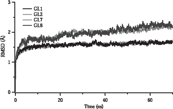
RMSD of VP1 in complexes over time. Each data are the average of three repetitive MD simulations. MD, molecular dynamics; RMSD, root mean square deviation.

3.1.2. Hydrogen bonding

Hydrogen bonding is one of the most prominent interactions that hold protein–protein complexes intact. Thus, interruption in the hydrogen-bonding network between protein–protein complexes can be a strong indication for perturbation of the complex formation. Simulations show that mutations reduce the number of hydrogen bonds between VP1 and FAB5I2 in addition to significant fluctuations in bond formation over time (Fig. 3). Average number of hydrogen bonds in wild type VP1–FAB5I2 complex interface (IF) is 7.5. This is in complete agreement with the X-ray crystallographic data of 8 (Shanker et al., 2016). In contrast, this number in all the mutations is <5.5 (Supplementary Table S2), confirming the loss of H-bonds. The persistence of hydrogen bonding over time also significantly differs in the wild type from the mutations such that the number of hydrogen bonds in wild type complex remains the same while in mutants fluctuates drastically. These findings are altogether clear evidence of weakening in interaction upon mutations.

FIG. 3.

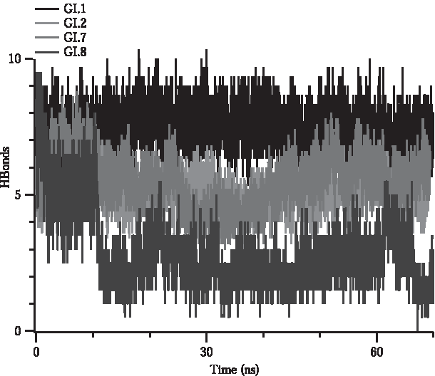
The number of H bonds formed between VP1 and FAB5I2 throughout MD simulations. Each data consist of the average of at least three repetitive MD simulations.

3.1.2.1. Interaction with CDRL1

In the wild type VP1–FAB5I2 complex, the most extensive H-bonding interactions are due to CDRL1 loop of FAB5I2, in which S28, L30, K32, and K35 are directly interacting with both Q-loop residues of T348, D350, and F352 and U-loop residues of N394, G396, and S398. Hence, we monitored specific distances among the interacting atoms corresponding to residues involved in critical H-bonding network. Figure 4 shows critical distances over time (time averaged data present on Supplementary Table S3).

FIG. 4.

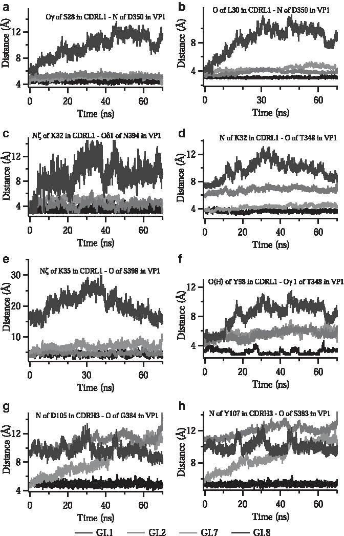
The distance between interacting atoms in critical residues over the course of MD simulations. Each data consist of the average of at least three repetitive MD simulations.

The Oγ of S28 and backbone O of L30 in the CDRL1 interact with the backbone N atom of D350. These distances do not alter significantly in GI.2 and GI.7 while they are completely removed in GI.8 (Fig. 4a, b).

Several atoms of K32 in the CDRL1 region are involved in strong H-bonding interactions with multiple residues of Q- and U-loops. The positively charged nitrogen (NH₃⁺, Nζ) of K32 side chain is distanced from Oδ1 and backbone O atoms of N394 by 3.2 and 2.8 Å, respectively (Fig. 4c; Supplementary Fig. S1). In addition, this Nζ of K32 in CDRL1 is in contact with backbone O atoms of F352 and G396 (Supplementary Fig. S1). These interactions are highly conserved in wild type GI.2 and GI.7 while disturbed in GI.8. Besides H-bonding, the charge on K32 also strengthens the VP1–FAB5I2 interaction due to contribution to the salt bridge formation on these residues. Not only the −NH₃⁺ side chain but the backbone N atom of K32 is also involved in H-bonding interaction with backbone O of T348, with the distance of 3.7 Å. This distance becomes greater and gains high mobility especially in GI.8 and GI.7 variants (Fig. 4d). Another H-bonding and salt bridge contributing residue is K35 in CDRL1. The Nζ atom of this residue is in proximity with O of S398 by only 3 Å (Fig. 4e).

3.1.2.2. Interaction with CDRL3

The involvement of CDRL3 in the VP1–FAB5I2 interaction is mostly through the H-bonding between O(H) atom of Y98 residue and Oγ1 of T348. Although this interaction fluctuates in all variants including wild type itself, distance becomes longer in mutants upon mutations (Fig. 4f).

3.1.2.3. Interaction with CDRH3

Experimental and computational data suggest that heavy chain of antibody, mostly through CDRH3, makes relatively weaker interaction with VP1 than light chain. The affinity of CDRH3 loop to VP1 is mostly driven by interactions among D105, Y107, and D108 residues in CDRH3; S383 and G384 residues in VP1 envelope protein. The backbone N atom of D105 residue is in proximity with backbone O atoms of S383 and G384 residues by 4.5 and 4.7 Å, respectively. These distances are within the limit of H-bond formation in the wild type, whereas they are totally diverged in all mutants (Fig. 4g). The distance between the backbone N of Y107 in CDRH3 and backbone O of S383 in VP1, 5.1 Å, is somewhat too far for H-bond interaction in wild type. However; this distance gets much worse in all mutations (Fig. 4h). The S383 on T-loop of VP1 also interacts with D108 in CDRH3 of FAB5I2. Through its backbone N and Oγ atoms, it makes quite strong two H-bonds with side chain carboxylate oxygen atoms (Oδ2 and Oδ1) of D108 with the distances of 3.3 and 2.8, respectively. Since S383 is mutated in all three mutants to Proline (in GI.2) and Alanine (in GI.7 and GI.8), the polar group on side chain of S383 is completely replaced by apolar groups resulting with H-bond disruptions in mutants.

In the GI.2 variant, most of the interactions of CDRs with Q- and U-loops were almost completely preserved since there is only a single mutation (N394D) on these regions and interacting atom of Oδ1 exists even after mutation (in both asparagine and aspartate). In contrast, in the GI.7 mutant, most of the residues in the Q-, T-, and U-loops are mutated. Thus, the interruption in the H-bond network is relatively large. The GI.8 variant, in which the mutations occurred mostly in the interacting loop regions, behaves very drastically due to the mutations and thus almost all the important distances were deviated from wild type. This result also can clearly be observed by the conformational instability throughout the MD simulations.

3.1.3. Root mean square fluctuation of epitope residues

Fluctuations in position of the residues are a direct result of disturbance of critical aforementioned interactions' network and complex formation. Comparing the mobility in T-, Q-, and U-loop residues of the VP1 proteins (Shanker et al., 2016), the wild type holds a very rigid conformation (∼1.5 Å), whereas those of the mutants oscillate ∼3.5 Å (Fig. 5). The level of fluctuation varies from one generation to another. The residues in the critical loops fluctuate mostly in GI.8 in comparison with all variants, whereas loops in GI.2 have the closest dynamic character to wild type VP1.

FIG. 5.

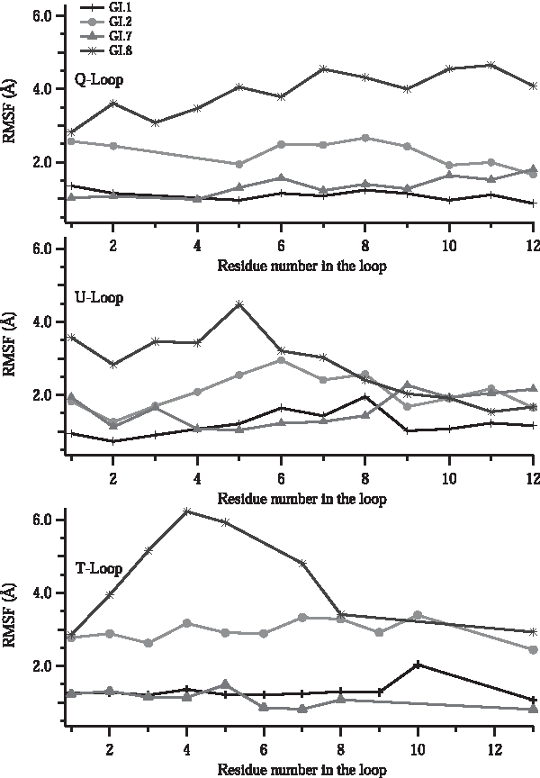
RMSF values of residues of the loops in the VP1–FAB5I2 complex IF. The numbering on x-axis refers to the position in the loop as also shown on top of Table 1. Each data consist of the average of at least three repetitive MD simulations. IF, interface; RMSF, root mean square fluctuation.

Mutations in each variant disturb different critical loops interacting with FAB5I2. Mutations in native virus genome that generate GI.8 lead fluctuation mostly in U-loop while T-loop gain high dynamic feature in all three generations (GI.2, GI.7, and GI.8). Similarly, Q-loop also fluctuates in all variants, but the level of fluctuation is the greatest in GI.8. This suggests that evolution during the life cycle of virus has different effect on the virus protein structure and results in diverse escape mechanism.

Table 1.

Loops and Blast Results

VP1	Q-loop														T-loop															U-loop
VP1		1	2	3	4	5	6	7	8	9	10	11	12			1	2	3	4	5	6	7	8	9	10	11	12	13			1	2	3	4	5	6	7	8	9	10	11	12
GI.1	345	V	D	–	–	T	T	P	D	T	F	V	P	354	377	S	P	P	S	H	P	S	G	S	Q	–	–	V	387	394	N	Y	G	S	S	I	T	E	A	T	H	L	405
GI.2	345	V	S	–	–	T	N	P	Q	G	F	V	P	354	377	S	P	P	S	T	P	P	G	S	Q	–	–	V	387	394	D	Y	G	S	S	I	T	E	A	T	H	L	405
GI.7	352	L	D	–	V	K	Q	N	A	P	F	A	P	362	387	S	P	S	T	S	G	A	R	–	–	–	–	V	395	402	S	Y	G	S	T	V	T	E	S	T	H	L	413
GI.8	354	V	V	I	H	S	Y	D	A	T	F	A	P	365	394	S	N	R	T	G	–	A	T	–	–	–	–	L	401	408	N	Y	G	S	N	L	T	Q	A	S	Q	L	419

	CDRL1																			CDRL3											CDRH3
FAB5I2	24	K	S	S	Q	S	V	L	Y	K	S	D	K	K	N	Y	L	A	40	96	Q	Y	Y	S	I	P	R	T	103	97	A	S	N	R	A	N	R	A	D	D	Y	D	Y	Y	F	D	Y	113

CDR, complementarity determining region.

3.1.4. Loop dynamics

In addition to fluctuation in critical residues that form complex IF, proximity of loops to each other is also crucial for complex formation since the affinity of VP1 to FAB5I2 is mostly gained by the loop interactions. Therefore, we monitored and compared the distances among the center of masses of loops that comprise the critical residues over time course of simulation. Mutations force these loops to stay in greater distance when compared with wild type VP1–FAB5I2 complex (Fig. 6). From the wild type to mutants, once an interaction is broken, all residues around the interaction get affected resulting with the move of the whole loop.

FIG. 6.

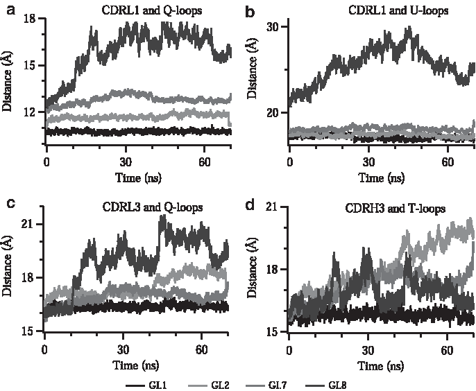
COM-to-COM distances between the loops. Each data consist of the average of at least three repetitive MD simulations. COM, center of mass.

Upon mutation, the distance between CDRL1 and Q-loop (Fig. 6a) in the GI.8 variant is affected the most, which shifts ∼5 Å from that of wild type, although other mutants were also affected by ∼2 Å shifts. Despite the fact that the distance between CDRL1 and Q-loop becomes greater in GI.2 and GI.7, this distance does not fluctuate over time (Fig. 6a). This might suggest that a new interaction network is established in their last conformations. Similar effect with less deviation in GI.2 and GI.7 is observed in the distance of CDRL1 to U-loop (Fig. 6b). The effect of mutation is more obvious in the distances of CDRL3 to Q-loops and CDRH3 to T-loop. The wild type GI.1 keeps very stable and unchanged distance over the course of simulation, whereas all mutants oscillate and diverge (Fig. 6c, d). Although there is no direct interaction of T-loop with the loops of CDRL1 and CDRL3, there is still a good response to mutation on these distances (Supplementary Fig. S3). This might suggest indirect interactions such as water-mediated interactions or hydrophobic interactions between these loops.

These results support that mutations do not only cause high fluctuation of critical residues, but they also force these residues to a further distance, which contributes emergence of lower affinity.

3.1.5. Solvent accessible surface area analysis

To understand how the contact surface area of VP1 and FAB5I2 changes upon mutation, we analyzed solvent accessible surface area (SASA) of IF. The more VP1 interacts with FAB5I2, the greater the IF area the complex has. To find SASA of IF throughout MD simulations, we obtained complex surface area (VP1–FAB5I2) and individual protein surface areas of VP1 and FAB5I2, then subtracted the complex area from the sum of individual protein areas as illustrated in Figure 7.

FIG. 7.

Illustration of IF area calculation from the surface areas of VP1, FAB5I2, and VP1–FAB5I2 complex in the MD simulations of the complex.

Figure 8 shows the total area of VP1–FAB5I2 complex and the area of IF throughout MD simulations. The total area of complex is the least in the case of wild type, confirming that it is the most compact structure and most of the IF is buried. The IF area in the wild type is persistent and greater than the areas in mutations. At the beginning of MD simulations, all the variants have similar IF areas. This is normal since we intentionally build the complexes of mutations by superimposing the FAB5I2 part from the wild type. Within the first 10 ns, the mutants start deviating from their first conformations, suggesting interaction loss and searching for better (minimum energy) conformation. In GI.8, VP1 completely loses the connection with FAB5I2, suggesting a strong escape mechanism upon mutations. Although GI.2 is generated by point mutations in just a few residues in the loops of wild type, the IF area over time gets affected substantially. This might be evident that the position of mutation is more important than the number of mutations in the escape mechanism.

FIG. 8.

SASA of (a) VP1–FAB5I2 complex and (b) complex IF calculated by Figure 7. Each data consist of average of at least three repetitive MD simulations. SASA, solvent accessible surface area.

3.2. Binding free energies

Free energy calculations are widespread methods for determination of binding affinity. However, they are computationally too costly and time consuming in particular in the case of protein–protein interactions. In contrast, the MM-PBSA method has been shown to be reasonably accurate in calculation of relative binding energies and is much more affordable in terms of computational cost and CPU times. Thus, we calculated the affinity of FAB5I2 to VP1 proteins by the MM-PBSA binding free energies (ΔΔG). The binding free energies presented in Table 2 clearly show that upon mutations, the affinity of FAB5I2 therapeutic antibody to VP1 drops drastically. The binding of FAB5I2 in the wild type VP1 is the strongest with 77.8 ± 1.9 kcal/mol and almost twice larger than the mutations. Interestingly, the mutant G I.2 has the lowest relative binding energy although its sequence in the interaction region is the closest to the wild type. This might be an indication that the location of the mutation is more important than the quantity of the mutations. The role of each loop in complex formation was further interrogated by determining the contribution of each loop in binding energy individually. Although the DDG values are not in harmony with root mean square fluctuation, RMSD, distance, and loop dynamics data, the contribution from each loop in the VP1 variants reflects the same pattern and the data are discussed in Section 3.1.

Table 2.

MM-PBSA Binding Free Energies of VP1 to FAB5I2 and Contributions of Each Loop in the Binding

Genotype	BE	SE	ΔΔG	Q-loop	T-loop	U-loop
GI.1	−77.8	1.9	0.0	−16.9	−8.9	−10.9
GI.2	−33.6	2.1	44.2	−6.0	−7.3	−3.9
GI.7	−46.6	2.3	31.2	−4.2	−2.3	−8.6
GI.8	−40.1	2.3	37.7	−3.2	0.0	−0.2

All values are in kcal/mol.

ΔΔG, relative energy; BE, binding energy; SE, standard error.

4. Conclusions

In this study, we investigated the effect of mutations on genogroup I and genotype 1 (GI.1) of NV. We performed several MD simulations on mutations that are hypothetically complexed with Fab fragment of a human IgA monoclonal antibody (FAB5I2) drug molecule as in the case of GI.1. The complex is found to be held intact mostly by the interactions of Q-, T-, and U-loops in VP1 and CDRL1, CDRL3, and CDRH3 loops in FAB5I2. MD simulation data suggested that all the mutations develop escape mechanism toward the FAB5I2 antibody upon mutations. Among them, the effect of mutation GI.8 is the most severe. In addition, the location of the mutation seems more important than the number of mutations. Free energy calculations also show the affinity loss upon mutation. We further analyzed individual residues of VP1 and FAB5I2 that are interacting and found that K32 and K35 in CDRL1, Y98 in CDRL3, and Y107 and D108 in CDRH3 are the key residues in FAB5I2 in binding to VP1. Among them, K32 is the most critical with multiple complex H-bond network. Mutations in VP1 residues that are in proximity to these residues can adapt to antibody. Corresponding residues in VP1 of GI.1 are T348 and D350 in Q-loop; S383 in T-loop; and N394, G396, and S398 in U-loops.

Footnotes

Acknowledgment

The numerical calculations reported in this article were partially performed at TUBITAK ULAKBIM, High Performance and Grid Computing Center (TRUBA resources). This research did not receive any specific grant from funding agencies in the public, commercial, or not-for-profit sectors.

Author Disclosure Statement

The authors declare that no competing financial interests exist.

References

Abraham

M.J.

, Murtola

, Schulz

, et al. 2015. GROMACS: High performance molecular simulations through multi-level parallelism from laptops to supercomputers. SoftwareX. 1–2, 19–25.

Aliabadi

, Lopman

B.A.

, Parashar

U.D.

, et al. 2015. Progress toward norovirus vaccines: Considerations for further development and implementation in potential target populations. Expert. Rev. Vaccines. 14, 1241–1253.

Baker

N.A.

, Sept

, Joseph

, et al. 2001. Electrostatics of nanosystems: Application to microtubules and the ribosome. Proc. Natl. Acad. Sci. U. S. A. 98, 10037–10041.

Belliot

, Lopman

B.A.

, Ambert-Balay

, et al. 2014. The burden of norovirus gastroenteritis: An important foodborne and healthcare-related infection. Clin. Microbiol. Infect. 20, 724–730.

Bernstein

D.I.

, Atmar

R.L.

, Lyon

G.M.

, et al. 2015. Norovirus vaccine against experimental human GII.4 virus illness: A challenge study in healthy adults. J. Infect. Dis. 211, 870–878.

Bull

R.A.

, Eden

J.S.

, Rawlinson

W.D.

, et al. 2010. Rapid evolution of pandemic noroviruses of the GII.4 lineage. PLoS Pathog. 6, e1000831.

Caddy

, Breiman

, le Pendu

, et al. 2014. Genogroup IV and VI canine noroviruses interact with histo-blood group antigens. J. Virol. 88, 10377–10391.

Darden

T.A.

, York

, and Pedersen

1993. J. Chem. Phys. 98, 10089.

Debbink

, Lindesmith

L.C.

, Donaldson

E.F.

, et al. 2013. Emergence of new pandemic GII.4 Sydney norovirus strain correlates with escape from herd immunity. J. Infect. Dis. 208, 1877–1887.

10.

de Graaf

, van Beek

, and Koopmans

M.P.

2016. Human norovirus transmission and evolution in a changing world. Nat. Rev. Microbiol. 14, 421–433.

11.

DeLano

W.L.

2002. The PyMOL Molecular Graphics System. Delano Scientific, San Carlos, CA.

12.

Emsley

, and Cowtan

2004. Coot: Model-building tools for molecular graphics. Acta. Crystallogr. D. Biol. Crystallogr. 60(12 Part 1), 2126–2132.

13.

Garaicoechea

, Aguilar

, Parra

G.I.

, et al. 2015. Llama nanoantibodies with therapeutic potential against human norovirus diarrhea. PLoS One. 10, e0133665.

14.

Hoa Tran

T.N.

, Trainor

, Nakagomi

, et al. 2013. Molecular epidemiology of noroviruses associated with acute sporadic gastroenteritis in children: Global distribution of genogroups, genotypes and GII.4 variants. J. Clin. Virol. 56, 185–193.

15.

Kambhampati

, Koopmans

, and Lopman

B.A.

2015. Burden of norovirus in healthcare facilities and strategies for outbreak control. J. Hosp. Infect. 89, 296–301.

16.

Karst

S.M.

, Zhu

, and Goodfellow

I.G.

2015. The molecular pathology of noroviruses. J. Pathol. 235, 206–216.

17.

Karst

S.M.

, Wobus

C.E.

, Goodfellow

I.G.

, et al. 2014. Advances in norovirus biology. Cell. Host. Microbe. 15, 668–680.

18.

Kocak

, Erol

, Yildiz

, et al. 2016. Computational insights into the protonation states of catalytic dyad in BACE1-acyl guanidine based inhibitor complex. J. Mol. Graph. Model. 70, 226–235.

19.

Kocak

, and Yildiz

2017. Docking, molecular dynamics and free energy studies on aspartoacylase mutations involved in Canavan disease. J. Mol. Graph. Model. 74, 44–53.

20.

Kotloff

K.L.

, Nataro

J.P.

, Blackwelder

W.C.

, et al. 2013. Burden and aetiology of diarrhoeal disease in infants and young children. Lancet. 382, 209–222.

21.

Kubota

, Kumagai

, Ito

, et al. 2012. Structural basis for the recognition of Lewis antigens by genogroup I norovirus. J. Virol. 86, 11138–11150.

22.

Kumari

, Kumar

, and Lynn

2014. g_mmpbsa—A GROMACS tool for high-throughput MM-PBSA calculations. J. Chem. Inform. Model. 54, 1951–1962.

23.

Lindesmith

L.C.

, Beltramello

, Donaldson

E.F.

, et al. 2012. Immunogenetic mechanisms driving norovirus GII.4 antigenic variation. PLoS Pathog. 8, e1002705.

24.

Lindorff-Larsen

, Piana

, Palmo

, et al. 2010. Improved side-chain torsion potentials for the Amber ff99SB protein force field. Proteins. 78, 1950–1958.

25.

Lochridge

V.P.

, Jutila

K.L.

, Graff

J.W.

, et al. 2005. Epitopes in the P2 domain of norovirus VP1 recognized by monoclonal antibodies that block cell interactions. J. Gen. Virol. 86(Pt 10), 2799–2806.

26.

Olsson

M.H.M.

, Søndergaard

C.R.

, Rostkowski

, et al. 2011. PROPKA3: Consistent treatment of internal and surface residues in empirical pKa predictions. J. Chem. Theory Comput. 7, 525–537.

27.

Patel

M.M.

, Hall

A.J.

, Vinje

, et al. 2009. Noroviruses: A comprehensive review. J. Clin. Virol. 44, 1–8.

28.

Robilotti

, Deresinski

, and Pinsky

B.A.

2015. Norovirus. Clin. Microbiol. Rev. 28, 134–164.

29.

Rocha-Pereira

, Neyts

, and Jochmans

2014. Norovirus: Targets and tools in antiviral drug discovery. Biochem. Pharmacol. 91, 1–11.

30.

Ruvoen-Clouet

, Belliot

, and Le Pendu

2013. Noroviruses and histo-blood groups: The impact of common host genetic polymorphisms on virus transmission and evolution. Rev. Med. Virol. 23, 355–366.

31.

Sapparapu

, Czako

, Alvarado

, et al. 2016. Frequent use of the IgA isotype in human B cells encoding potent norovirus-specific monoclonal antibodies that block HBGA binding. PLoS Pathog. 12, e1005719.

32.

Schrödinger

2015. Maestro. Schrödinger Release 2015-2. Schrödinger, LLC, New York, NY.

33.

Shanker

, Czako

, Sankaran

, et al. 2014. Structural analysis of determinants of histo-blood group antigen binding specificity in genogroup I noroviruses. J. Virol. 88, 6168–6180.

34.

Shanker

, Czako

, Sapparapu

, et al. 2016. Structural basis for norovirus neutralization by an HBGA blocking human IgA antibody. Proc. Natl. Acad. Sci. U. S. A. 113, E5830–E5837.

35.

Tamminen

, Malm

, Vesikari

, et al. 2016. Mucosal antibodies induced by intranasal but not intramuscular immunization block norovirus GII.4 virus-like particle receptor binding. Viral. Immunol. 29, 315–319.

36.

Tan

, and Jiang

2014. Vaccine against norovirus. Hum. Vaccin. Immunother. 10, 1449–1456.

37.

Toukan

, and Rahman

1985. Molecular-dynamics study of atomic motions in water. Phys. Rev. B. 31, 2643–2648.

38.

White

P.A.

2014. Evolution of norovirus. Clin. Microbiol. Infect. 20, 741–745.

Supplementary Material

Please find the following supplemental material available below.

For Open Access articles published under a Creative Commons License, all supplemental material carries the same license as the article it is associated with.

For non-Open Access articles published, all supplemental material carries a non-exclusive license, and permission requests for re-use of supplemental material or any part of supplemental material shall be sent directly to the copyright owner as specified in the copyright notice associated with the article.

0.00 MB

0.45 MB

0.96 MB

0.02 MB