Three-Dimensional Embryonic Image Segmentation and Registration Based on Shape Index and Ellipsoid-Fitting Method

Abstract

Quantitative analysis based on three-dimensional differential interference contrast (DIC) images is currently the mainstream in analyzing gene functions involved in early cell fate specifications. Segmentation and registration are the two most important steps in analysis. Many image segmentation methods have poor performance on embryonic DIC images because of the interference of egg shells, blurs, and nonuniform intensity background. A novel segmentation method is presented based on the shape index (SI) of local intensity variation in DIC images. To compute the SI, the intensity values of a local neighborhood are regarded as z coordinates over x–y planes. After calculating the SI for each pixel by evaluating the shape of intensity surface over the corresponding local neighborhood, SI thresholding is used to detect cytoplasm granules within embryonic boundaries. As a scalar and rotation invariant, the SI is both insensitive to directional changes and different ranges of intensity variations. Embryonic registration methods are usually based on the orientation of vertebrate anteroposterior (AP) axes computed from segmented embryonic boundaries. Due to the blur of marginal slices in DIC images, usually the segmented boundaries are incomplete, which may make the computed AP axes shift away from the correct orientation when using the principal component analysis method. A method calculating AP axes based on ellipsoid-fitting is proposed, which can achieve high accuracy when handling incomplete segmented boundaries. Using Worm Developmental Dynamics Database, we evaluated the performance of the proposed segmentation method and the computation of AP axes. Experimental results show that the two methods outperform existing methods.

1. Introduction

In recent years, RNA interference (RNAi) and differential interference contrast (DIC) imaging techniques are emerging as essential tools to assist biologist in analyzing embryonic development, morphology, and phenotypes in single-cell level. The large number of images produced in these studies makes manual analysis intractable. Hence, automatic cellular image processing and analysis becomes an important task. To automatically analyze the nuclear development in a four-dimensional (4D) way based on a series of three-dimensional (3D) DIC images obtained at different time points, image segmentation and registration are the two necessary steps. For 3D embryonic images, the registration is usually based on the orientation of anteroposterior (AP) axes. Principal component analysis (PCA) is the mainly applied method to compute AP axes. Before using PCA, it is needed to segment embryonic boundaries in images.

In this article, we present a novel scheme on cellular boundary segmentation. Furthermore, an ellipsoid-fitting scheme is used to build models for embryonic boundaries according to the segmented incomplete boundaries. Based on the fitted ellipsoid models, the AP axes are computed and the registration is carried out.

Based on the shape index (SI), the proposed segmentation method focuses on the detection of cytoplasm granules inside the cellular regions in each slice of a 3D embryonic image. Because the size of the cytoplasm granules is usually too small compared with the thickness of focal planes in the z-stack, we could not calculate the SI by using the method of constructing the intensity isosurface in 3D images. Consequently, we regard intensity as Z coordinate and compute the SI within each slice. An SI value is computed to represent the shape of intensity surface near to a target pixel. With several geometric postprocessing techniques, the SI thresholding results are integrated into a boundary in each slice. Experimental results show that the proposed algorithm has higher accuracy than existing schemes despite the existence of egg shells with different shapes and fluctuated intensities.

On the computation of AP axes, PCA works well when the contour of an embryo is obtained entirely. However, because of the existence of blur in marginal slices of 3D DIC images, using image segmentation methods usually could not obtain correct boundaries in these slices. Therefore, these slices are often discarded, which will make the final segmented boundaries incomplete and missing on the margins of z-stack. When the segmented boundaries are incomplete, the AP axis calculated from PCA may shift away from the correct orientation. Therefore, we used the ellipsoid-fitting method to compute AP axes in this article, which can calculate the correct value even when the segmented boundaries are incomplete. A preliminary result of segmentation was presented in an international conference (Yang et al., 2017).

The remainder of this article is organized as follows. In Section 2, the proposed segmentation algorithm based on the SI is described in detail. Experimental results on segmentation algorithms to be compared are presented in Section 3. Section 4 demonstrates the ellipsoid-fitting method on the calculation of AP axes. In Section 5, we experimentally compared the computed AP axes using the ellipsoid-fitting method and PCA. Finally, Section 6 concludes the article.

2. DIC Embryonic Image Segmentation based on the SI

In DIC images, it is difficult to obtain robust and accurate cellular boundaries by automatic image segmentation methods. First, microscopy images are often with many blurs, nonuniform intensity backgrounds. The contrast also varies between the foreground and the background. Second, the size, shape, and location of cells are usually different. Finally, the existence of egg shells interferes the detection of correct boundaries.

A large number of algorithms have been developed for automatic or semi-automatic cellular segmentation (Irshad et al., 2013; Xing and Yang, 2016). These methods are based on a few basic approaches: intensity thresholding, feature detection, morphological filtering, and deformable model fitting (Meijering, 2012). Learning-based schemes are also proposed in cell segmentation tasks. A notable work is the five categories of segmentation system in cellular regions (Ning et al., 2005). However, the learning-based methods require labeling samples manually for training, and it is a time-consuming and labor-intensive task. Consequently, we focused on the nonlearning-based schemes in this study.

Although some adaptive thresholding techniques are presented (Bradley and Roth, 2007), thresholding methods are prone to be influenced by nonuniform background. Methods based on morphological filtering, especially watershed techniques, are widely used in cell segmentation (Adiga and Chaudhuri, 2001; Lin et al., 2003). Nevertheless, it performs well in the segmentation of touching cells, and the existence of egg shells makes it tricky in our case. Deformable models and the related algorithms are also widely applied in biomedical image segmentation (McInerney and Terzopoulos, 1996). However, when they are used in raw images, their performances are restricted. Schemes based on the feature detection are different and flexible, but they lack the overall control of the boundaries in general.

Kyoda et al. (2013) proposed an effective segmentation method based on entropy filter and the classic active contour method. They also applied the segmented nuclei to trace the development of nuclei. Although their method performs well in nuclear segmentation, its accuracy still suffers the nonuniform of background intensity when applying to cellular boundary segmentation.

2.1. The segmentation method based on the SI

The SI is a descriptor to quantify the pure shape of a two-dimensional (2D) surface. It was proposed by Koenderink and Doorn (1992). Its computational formula is shown in Equation (1). Here, κ₁ and κ₂ are two principal curvatures of the surface. \documentclass{aastex}\usepackage{amsbsy}\usepackage{amsfonts}\usepackage{amssymb}\usepackage{bm}\usepackage{mathrsfs}\usepackage{pifont}\usepackage{stmaryrd}\usepackage{textcomp}\usepackage{portland, xspace}\usepackage{amsmath, amsxtra}\usepackage{upgreek}\pagestyle{empty}\DeclareMathSizes{10}{9}{7}{6}\begin{document} \begin{align*} S = \frac { 2 } { \pi } \arctan { \frac { { \kappa _2 } + { \kappa _1 } } { { \kappa _2 } - { \kappa _1 } } } , \quad { \kappa _1 } \ge { \kappa _2 } , \quad S = \left[ { - 1 , 1 } \right]. \tag { 1 } \end{align*} \end{document}

Based on their original work, researchers developed many techniques. Cantzler and Fisher (2001) exhaustively compared the properties of the Gaussian curvature, mean curvature, and SI. Dorai and Jain (1997) established a linkage between the SI and Gaussian mapping and creatively proposed shape spectrum to accumulate morphological information. Huibin et al. (2011) studied the histogram of SI values and used it as a descriptor to identify facial expression. Yang et al. (2016) showed an equivalent formula on the SI and deduced the counterpart formula when there are three principal curvatures to be considered based on spherical coordinate system. Yoshida and Näppi (2001) applied SI to the detection of colonic polyps in 3D images based on the intensity isosurface. Their work is adopted in many biomedical diagnostic software packages. As shown in Figure 1a, there are many cytoplasm granules in cellular regions. For each cytoplasm granule in a 2D slice, the intensity surface (Fig. 1b) is close to a “cap,” whereas for a pixel surrounded by cytoplasm granules, the intensity surface is similar to a “cup.” Therefore, the SI can be used to detect these featured local regions.

FIG. 1.

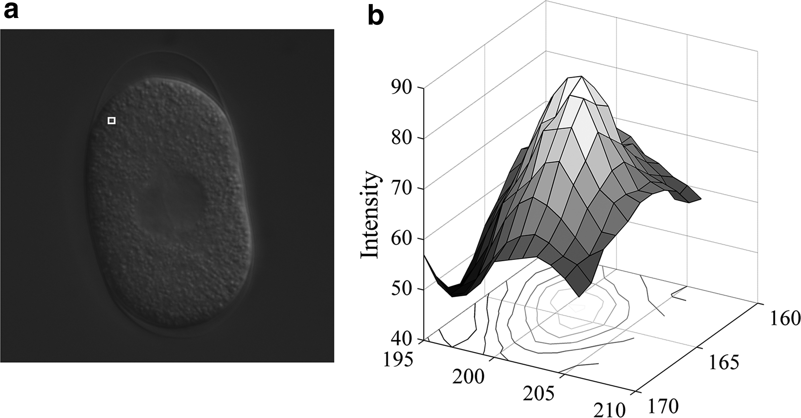
A sample cell slice. (a) Cell slice with manually segmented boundary (in white color). (b) The intensity surface of the tiny block in (a).

2.2. The proposed algorithm

To obtain the segmented embryonic boundaries, the following steps are applied on each 4D DIC image:

Step 1. For each 2D slice I_t,_n (n: slice number and t: time), use a 11 × 11 Gaussian kernel to smooth the slice.

Step 2. For each pixel in I_t,_n, compute the Gaussian curvature K and mean curvature H in its 7 × 7 neighborhood and then calculate the two principal curvatures κ₁, κ₂, the SI value S, and curvedness C.

Step 3. Set S = 0 for pixels with C < TH_C, then threshold I_t,_n based on |S| ≥ TH_S.

Step 4. Use geometric postprocessing techniques to obtain the final segmentation results.

In the rest of this section, the four steps are demonstrated in detail. Figure 2 shows the scheme of the proposed algorithm.

FIG. 2.

The procedure of the presented algorithm.

2.2.1. Initializing

In Step 1, t is the order of time points and n is the order of z-stack. A pair of t and n defines a 2D slice. The data set and its format are introduced in Section 3.1. For reducing noise, we used the Gaussian kernel to smooth each slice before computing S.

2.2.2. The computation of SI

In the presented algorithm, Steps 2–3 are related to the computation of SI. When detecting colonic polyps, Yoshida and Näppi (2001) used an SI value S to represent the local shape of the intensity isosurface of a voxel based on the approach of Thirion and Gourdon (1995). From this point of view, for each voxel in a 3D image, we can determine only one isosurface and calculate two principal curvatures within its neighborhood. An SI value S thus can be calculated. This method is appropriate to detect voxels located on a surface, which is distinguishable from background on space and intensity. In their study, the size of colonic polyps to be detected ranges from 5 to 30 mm and the interval of rebuilt 3D images is 1.5–2.5 mm (Yoshida and Näppi, 2001). Thus, their scheme is an appropriate way to characterize the shape of colonic polyps.

However, when detecting cytoplasm inside cellular boundaries, using z coordinate is futile because the radii are about 0.4–0.6 μm, whereas the interval of the acquired 3D images is 0.5 μm on z coordinate. As a result, it is hard to observe isosurface on z coordinate for most of the cytoplasm granules.

For using the SI in each slice to describe the variation of local intensity, we directly regard the intensity as z coordinate and calculate the two principal curvatures from the intensity surface for a neighborhood region of a pixel (Peet and Sahota, 1985). For the computation of principal curvatures, the method described by Besl and Jain (1986) was used. Suppose f (x,y) is the intensity surface over image planes (x,y), based on the first and second partial derivatives f_x, f_y, f_xx, f_yy, f_xy, we calculate the Gaussian curvature and mean curvature with Equation (2) at first and then obtain Equation (4) according to Equation (3) to compute the SI value S and the curvedness value C. In Step 3, TH_S and TH_C are thresholds of S and C, respectively, here are 0.68 and 0.05. To improve the computational accuracy, the computation is based on an interpolated neighborhood as discussed later in this section. \documentclass{aastex}\usepackage{amsbsy}\usepackage{amsfonts}\usepackage{amssymb}\usepackage{bm}\usepackage{mathrsfs}\usepackage{pifont}\usepackage{stmaryrd}\usepackage{textcomp}\usepackage{portland, xspace}\usepackage{amsmath, amsxtra}\usepackage{upgreek}\pagestyle{empty}\DeclareMathSizes{10}{9}{7}{6}\begin{document} \begin{align*} K = { \frac { { f_ { xx } } { f_ { yy } } - f_ { xy } ^2 } { { { ( 1 + f_x^2 + f_y^2 ) } ^2 } } } , \quad H = { \frac { { f_ { xx } } + { f_ { yy } } + { f_ { xx } } f_y^2 + { f_ { yy } } f_x^2 - 2 { f_x } { f_y } { f_ { xy } } } { { { ( 1 + f_x^2 + f_y^2 ) } ^ { { 3 \mathord { \left/ { \vphantom { 3 2 } } \right. \kern- \nulldelimiterspace } 2 } } } } } . \tag { 2 } \end{align*} \end{document} \documentclass{aastex}\usepackage{amsbsy}\usepackage{amsfonts}\usepackage{amssymb}\usepackage{bm}\usepackage{mathrsfs}\usepackage{pifont}\usepackage{stmaryrd}\usepackage{textcomp}\usepackage{portland, xspace}\usepackage{amsmath, amsxtra}\usepackage{upgreek}\pagestyle{empty}\DeclareMathSizes{10}{9}{7}{6}\begin{document} \begin{align*} { \kappa _{1 , 2}} = H \pm \sqrt {{H^2} - K}. \tag{3} \end{align*} \end{document} \documentclass{aastex}\usepackage{amsbsy}\usepackage{amsfonts}\usepackage{amssymb}\usepackage{bm}\usepackage{mathrsfs}\usepackage{pifont}\usepackage{stmaryrd}\usepackage{textcomp}\usepackage{portland, xspace}\usepackage{amsmath, amsxtra}\usepackage{upgreek}\pagestyle{empty}\DeclareMathSizes{10}{9}{7}{6}\begin{document} \begin{align*} S = \frac { 2 } { \pi } \arctan \left( { \frac { H } { { \sqrt { { H^2 } - K } } } } \right) , \quad { \kappa _1 } \ge { \kappa _2 } , \quad C = \sqrt { \frac { 1 } { 2 } \left( { \kappa _1^2 + \kappa _2^2 } \right) } = \sqrt { 2 { H^2 } - K } . \tag { 4 } \end{align*} \end{document}

2.2.3. SI images

Figure 3 shows the SI computational results under this viewpoint. After computing the SI for each pixel of a slice, we obtained the corresponding SI image (Figure 3a, b). Then, a threshold will be set to screen pixels with small SI value (Fig. 3c, d). From the result, we observed that when choosing an appropriate threshold, SI can simultaneously detect the cytoplasm granules and remove most of points on egg shells.

FIG. 3.

SI image. (a) SI image of a cell slice. (b) A patch of SI image. (c) The result of SI thresholding with TH_S as 0.5. (d) The result of SI thresholding with TH_S as 0.75. SI, shape index.

2.2.4. Geometric postprocessing techniques

After thresholding, we need to build masks from the detected points, as Step 4 shows. We used two steps to reach the goal.

First, along the direction from each boundary pixel P_b of a 2D slice to the central of the whole detected points by SI, we used a disk model to count the number of detected points (Fig. 4a) within the disk. If the number is less than a threshold, we removed these detected points. Once the detected points P_d within the disk is larger than a threshold, we constructed the convex hull of P_d (Fig. 4b).

FIG. 4.

Boundary construction based on SI detection result. (a) The searching process. (b) The way to merge the detected points to the final boundary using convex hulls. (c) A sketch map of L and D.

Second, we filled the image and then detected and removed occasional protrusions. Although choosing proper threshold of SI can mainly remove the interference caused by an egg shell, there may exist few detected points at its position and occasionally not be removed by the disk-searching step, which will bring protrusions, as shown in Figure 4c. To detect them, for each cellular boundary point P₁ generated by the filled image, let P₂ is another boundary point along a given direction, for example clockwise, when move P₂ and make the boundary length L between P₁ and P₂ ranging from L_min to L_max, a D/L ratio is calculated, here D is the Euclidean distance between P₁ and P₂. Once the ratio is less than a threshold, the piece of boundary is judged as a protrusion and a circular arc with radius 100 with the same x, y shifts is used to replace the boundary from P₁ to P₂.

3. Experiments on Embryonic Image Segmentation

3.1. Data set

The performance of our proposed scheme is evaluated on Worm Developmental Dynamics Database (WDDD) (Kyoda et al., 2013). Using 4D DIC microscopy, WDDD has 50 sets of quantitative data from wild type (WT) embryos. After silencing embryonic genes on chromosome III individually, 72 genes with 136 sets of quantitative data from RNAi experiments were also built (http://so.qbic.riken.jp/wddd). For each set, there are 180 time points (40 s/time point) and a 3D image is stored at each time point. In each 3D image, the z-stack includes 66 focal planes (0.5 μm/plane), and there are 600 × 600 pixels (0.105 μm/pixel) in each focal plane.

3.2. Evaluation of segmentation performance

To evaluate the performance of the proposed scheme, we chose 123 typical slices from 3 embryos (15th–55th in 66 slices) and manually segmented them as the ground truth. Then, we used entropy filter (Kyoda et al., 2013) and the distance regularized level set algorithm (EL algorithm; Li et al., 2010) as the comparison object. We also tested the scheme using the adaptive thresholding method according to Bradley and Roth (2007) and the morphological operators to segment cellular boundaries (TM algorithm). Besides, Watershed algorithm is also considered here. Table 1 shows the experimental results.

Table 1.

The Comparison of the Proposed Method with Other Algorithms

Method	Precision	Recall	Dice
EL algorithm	0.8943	0.9005	0.8974
TM algorithm	0.9657	0.9236	0.9442
Watershed algorithm	0.9419	0.8400	0.8880
Proposed algorithm	0.9737	0.9704	0.9721

EL, entropy filter and the distance regularized level set algorithm; TM, adaptive thresholding method and morphological operators.

3.3. Experimental results on different thresholds of SI

To evaluate the performance of the proposed method under different SI thresholds, we computed the segmentation results and the precision, recall, and dice ratio when SI changing from 0.55 to 0.90 with 0.05 as the step. Figure 5 shows the result. As shown in Figure 5, choosing 0.65–0.7 can obtain a balanced result in this study.

FIG. 5.

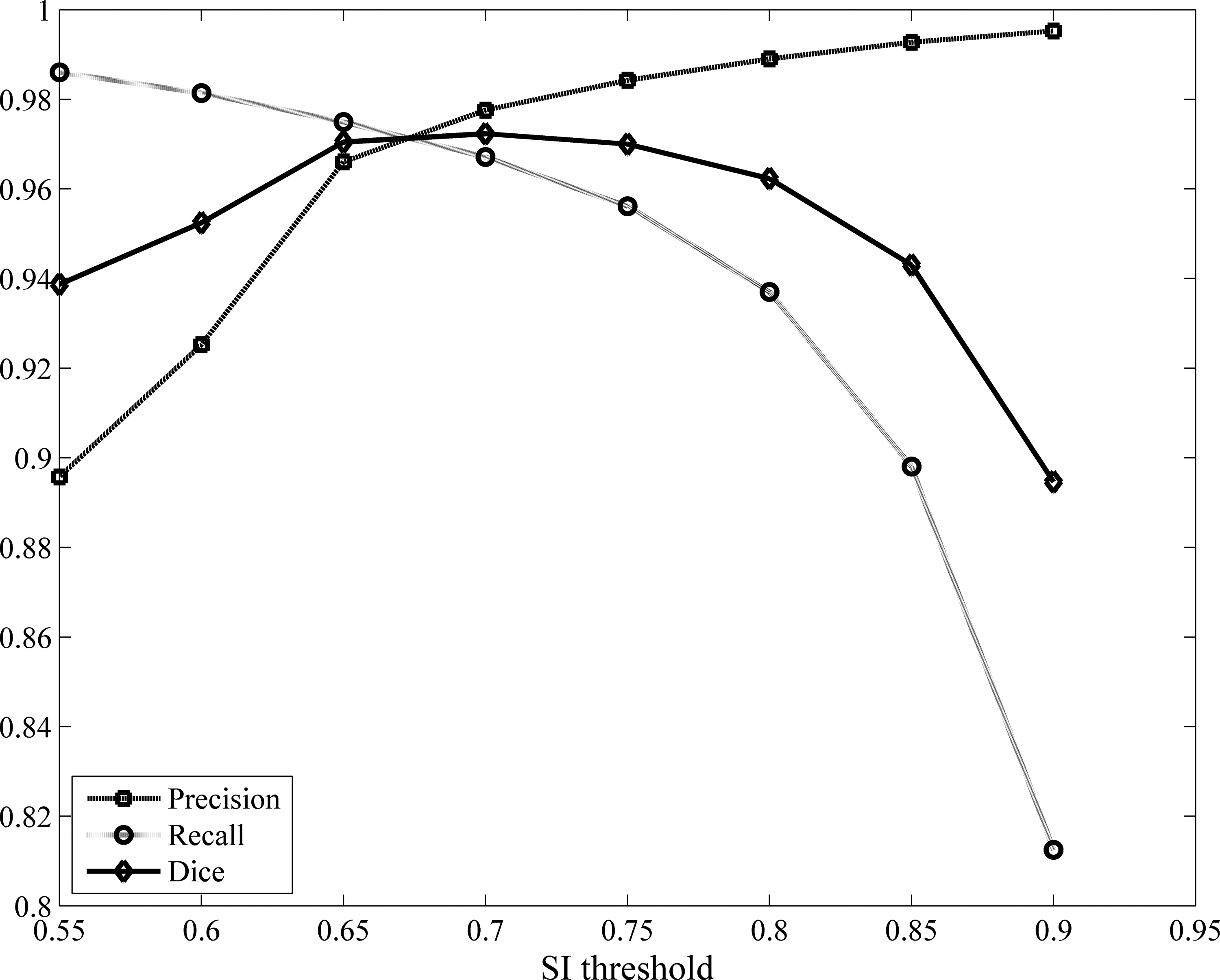
The comparison result when setting different SI thresholds.

3.4. Computational accuracy of the SI

In the computation of SI, the discretization of image may make the calculated value deviate from the correct value of the corresponding desire shape. To evaluate the accuracy of SI in practical computation, we build 5 ideal models of intensity shapes and the corresponding images. Then, we computed the SI from these images under different parameters and observed the difference between the calculated value and the theoretical one. In practical computation, the computational accuracy of SI is mainly related to the “resolution” of intensity shape, marked as RIS. When computing partial derivatives, the computational domain can be chosen as the same size of RIS.

Suppose there is a perfect intensity shape and it is a semi-sphere, when the intensity shape is discretized as RIS = 7 × 7, 9 × 9, … (having different “resolution”), the calculated values are slightly different. To observe the accuracy of computed SI under different resolutions, we build ideal models for SI = −1, −0.5, 0, 0.5, 1 (see Equation 5) and then discretized these models making RIS = 5 × 5, 7 × 7, …, as shown in Figure 6. After that, we computed the SI value at the center of these images. 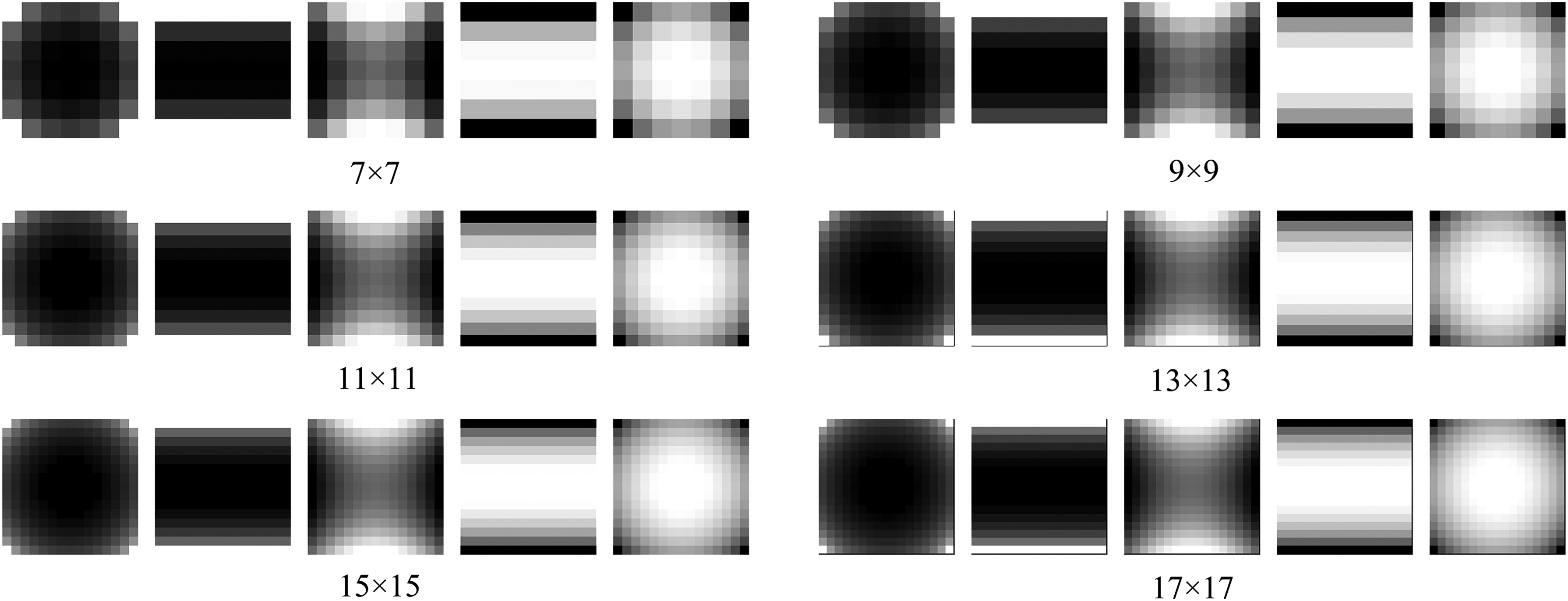\documentclass{aastex}\usepackage{amsbsy}\usepackage{amsfonts}\usepackage{amssymb}\usepackage{bm}\usepackage{mathrsfs}\usepackage{pifont}\usepackage{stmaryrd}\usepackage{textcomp}\usepackage{portland, xspace}\usepackage{amsmath, amsxtra}\usepackage{upgreek}\pagestyle{empty}\DeclareMathSizes{10}{9}{7}{6}\begin{document} \begin{align*} {I_{ - 1}} = - \sqrt {{r^2} - {x^2} - {y^2}} , \quad {I_{ - 0.5}} = - \sqrt {{r^2} - {x^2}} , \quad {I_0} = {x^2} - {y^2} , \quad {I_{0.5}} = \sqrt {{r^2} - {x^2}} , \quad {I_{ - 1}} = \sqrt {{r^2} - {x^2} - {y^2}}. \tag{5} \end{align*} \end{document}

FIG. 6.

The built models with different RIS. RIS, “resolution” of intensity shape.

By evaluating typical slices, we found the size of cytoplasm granules mainly ranging from 7 × 7 to 17 × 17. In comparison, we found that using larger RIS will increase the computational accuracy of SI. However, the real size of cytoplasm granules confines the maximal size we could use. Therefore, we used interpolation to enhance the resolution of both built models and real neighborhoods. After that, we used large RIS to compute the SI. Figure 7a shows the computational result when directly using the built model to compute the SI. Figure 7b shows the computational result when using cubic interpolation to obtain the interpolated models.

FIG. 7.

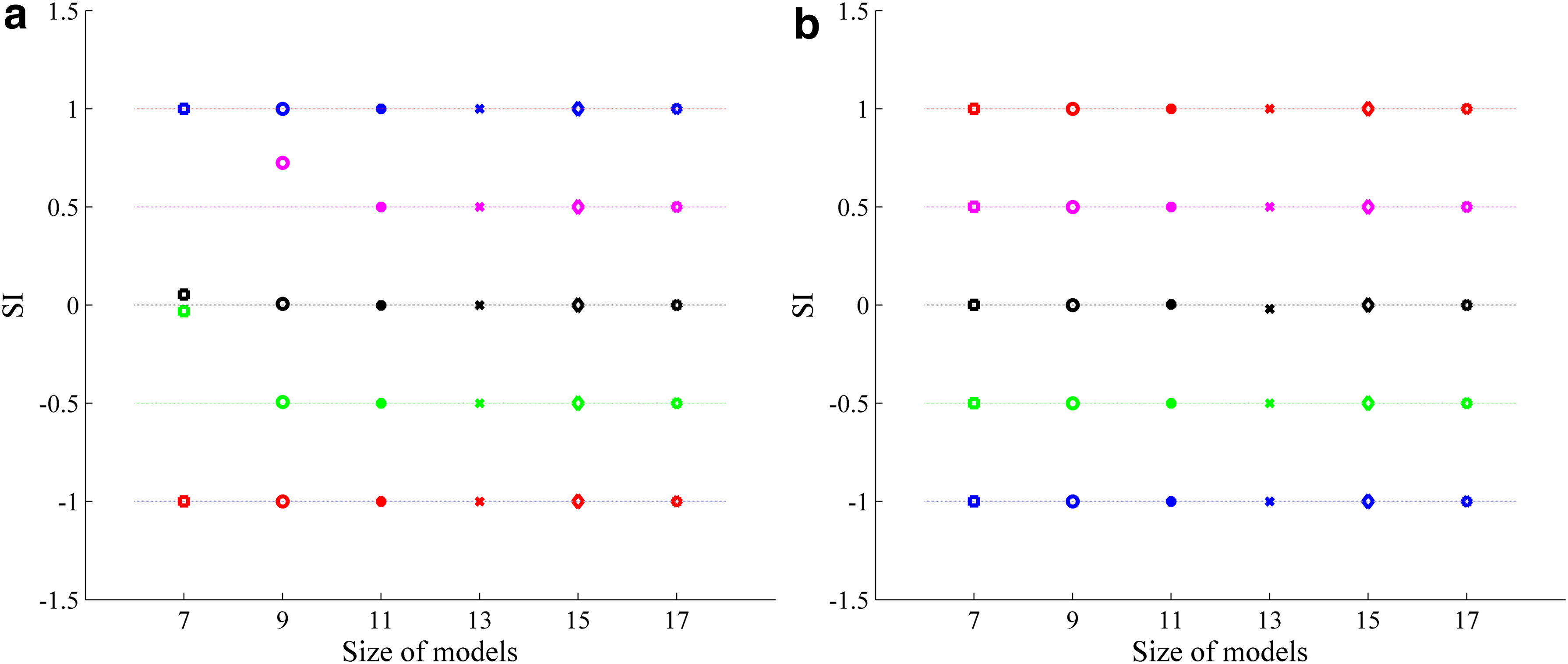
Computed SI before and after interpolation. (a) Computed SI within original neighborhood. (b) Computed SI within interpolated neighborhood.

3.5. Nuclear segmentation results

Using thresholding of the SI image with different thresholds and similar geometric methods, we segmented nuclear regions in DIC images. Figure 8 shows the segmentation result of a 3D image both on boundary and on nuclei.

FIG. 8.

Segmentation results on both the boundary and the nuclei of a 3D image. 3D, three-dimensional.

4. Estimation of AP Axes and 3D Embryonic Registration based on Ellipsoid-Fitting

In DIC imaging, usually the position of embryos is different. However, for each embryo, its egg shell is always oval and the main axis is AP axis. Furthermore, the AP axis will later develop to the body of Caenorhabditis. elegans, and one side is the head and the other side is tail. Therefore, usually, we used this characteristic to implement the registration.

4.1. The AP axes of embryos

PCA is widely used in computing AP axes. The eigenvector corresponding to the largest eigenvalue can be viewed as the main axis (AP axis). This method works well when the contour of an embryo is extracted entirely. However, when the segmented contours are incomplete, the AP axis calculated from PCA may shift away from the correct orientation (see Section 5.1). As we have mentioned, the DIC images are blur on the two marginal slices of z-stack, it is very difficult to automatically segment the correct boundary of embryos in these slices. Therefore, to facilitate the whole computation, we chose slices 15–53 to run the segmentation algorithm, whereas other slices are left blank.

To avoid the computational deviation of AP axes when using incompletely segmented boundaries, a reasonable scheme is to build a model for the whole boundary of an embryo according to the incomplete segmentation. Then, the model was used to calculate its AP axis. Based on empirical observation, we applied ellipsoids as the fitted model of embryonic boundaries.

There are two categories of ellipsoid-fitting methods. One is geometric fitting, which searches for the ellipsoid minimizing the sum of the square of the Euclidean distances between the given data set and the ellipsoid to be fitted. Another is algebraic fitting, which looks for the parameters of the ellipsoid f to minimize the sum of the Frobenius norm of f ( X ), here X is the given data set. Usually, the solving of geometric fitting requires iterative steps and is computationally expensive. Because the ellipsoid-fitting is extensively used in the study, we used algebraic fitting in this article.

The ellipsoid-fitting methods are the generalization of ellipse-fitting methods. Since the works of Bookstein (1979), Fitzgibbon and Fisher (1995), and Fitzgibbon et al. (1999), the computation of ellipse-fitting has been translated to the solving of a generalized eigenvalue system and there is a fixed procedure. However, the solving of ellipsoid-fitting in general cases is still a suspended problem. Qingde and Griffiths (2004) proposed an ellipsoid-fitting method, which is effective when the ratio of the major axis and other axes is not too large. The computation of this method is also fairly stable and fast. In this study, we used this method to compute the fitted ellipsoid and the corresponding AP axes.

4.2. The ellipsoid-fitting method

The procedure of fitting an ellipsoid is introduced in Qingde and Griffiths (2004). The steps for computing AP axes in our case are as follows: 1.

Segment original 3D images to obtain embryonic boundaries.

Build matrices D , C separately and set k = 4.

Compute the correlation matrix S based on D .

Compute the generalized inverse solution M from S .

Perform eigen-decomposition of M to obtain u , u is the eigenvector corresponding to the positive eigenvalue.

Build matrix P from u .

Perform eigen-decomposition of P to obtain the final AP axes.

In the above procedure, suppose the coordinates of voxels on the boundaries are [ x , y , z ], which include the whole boundary points [x_i, y_i, z_i], i = 1, 2, …, n and n is the number of boundary voxels. Then, the matrices D , C , S , M , P in the procedure are shown in Equations (6) and (7); S ₁₁ and S ₂₂ (6 × 6 and 4 × 4 matrices). The computed orientation of AP axis is just the eigenvector corresponding to the maximal eigenvalue of P . Figure 9 shows a 3D boundary and the corresponding fitted ellipsoid. \documentclass{aastex}\usepackage{amsbsy}\usepackage{amsfonts}\usepackage{amssymb}\usepackage{bm}\usepackage{mathrsfs}\usepackage{pifont}\usepackage{stmaryrd}\usepackage{textcomp}\usepackage{portland, xspace}\usepackage{amsmath, amsxtra}\usepackage{upgreek}\pagestyle{empty}\DeclareMathSizes{10}{9}{7}{6}\begin{document} \begin{align*} \textbf{\textit{D}} = { \rm{ }} \left[ {{\textbf{\textit{x}}^2} , {\textbf{\textit{y}}^2} , {\textbf{\textit{z}}^2} , { \rm{ }}2\textbf{\textit{yz}} , { \rm{ }}2 \textbf{\textit{xz}} , { \rm{ }}2 \textbf{\textit{xy}} , { \rm{ }}2 \textbf{\textit{x}} , { \rm{ }}2 \textbf{\textit{y}} , { \rm{ }}2 \textbf{\textit{z}} , { \bf{1}}} \right] , \tag{6} \end{align*} \end{document} \documentclass{aastex}\usepackage{amsbsy}\usepackage{amsfonts}\usepackage{amssymb}\usepackage{bm}\usepackage{mathrsfs}\usepackage{pifont}\usepackage{stmaryrd}\usepackage{textcomp}\usepackage{portland, xspace}\usepackage{amsmath, amsxtra}\usepackage{upgreek}\pagestyle{empty}\DeclareMathSizes{10}{9}{7}{6}\begin{document} \begin{align*} \textbf{\textit{C}} = \left[ { \begin{matrix} { - 1} & {{k \over 2} - 1} & {{k \over 2} - 1} & 0 & 0 & 0 \\ {{k \over 2} - 1} & { - 1} & {{k \over 2} - 1} & 0 & 0 & 0 \\ {{k \over 2} - 1} & {{k \over 2} - 1} & { - 1} & 0 & 0 & 0 \\ 0 & 0 & 0 & { - k} & 0 & 0 \\ 0 & 0 & 0 & 0 & { - k} & 0 \\ 0 & 0 & 0 & 0 & 0 & { - k} \\ \end{matrix} } \right] , \quad k = 4 , \quad \left\{ { \begin{matrix} {\textbf{\textit{S}} = {\textbf{\textit{D}}^T}\textbf{\textit{D}} = \left[ { \begin{matrix} {{\textbf{\textit{S}}_{11}}} & {{\textbf{\textit{S}}_{12}}} \\ {\textbf{\textit{S}}_{12}^T} & {{\textbf{\textit{S}}_{22}}} \\ \end{matrix} } \right] } \hfill \\ {} \hfill \\ {\textbf{\textit{M}} = {\textbf{\textit{C}}^{ - 1}} ( {\textbf{\textit{S}}_{11}} - {\textbf{\textit{S}}_{12}}\textbf{\textit{S}}_{22}^{ - 1}\textbf{\textit{S}}_{12}^T ) } \hfill \\ {} \hfill \\ {\textbf{\textit{P}} = \left[ { \begin{matrix} {{\textbf{\textit{u}}_1}} & {{\textbf{\textit{u}}_6}} & {{\textbf{\textit{u}}_5}} \\ {{\textbf{\textit{u}}_6}} & {{\textbf{\textit{u}}_2}} & {{\textbf{\textit{u}}_4}} \\ {{\textbf{\textit{u}}_5}} & {{\textbf{\textit{u}}_4}} & {{\textbf{\textit{u}}_3}} \\ \end{matrix} } \right] } \hfill \\ \end{matrix} } \right. \tag{7} \end{align*} \end{document}

FIG. 9.

The ellipsoid-fitting method based on incomplete boundaries. (a) Is segmented incomplete boundaries. (b) Is a fitted ellipsoid based on boundaries.

4.3. Interpolation

The fitting of ellipsoids can use segmented boundaries directly, and we do not need interpolation in the computation of AP axes. However, when constructing the registered images, we should conduct it by isotropic way. As we have mentioned in Section 3.1, the spans on x, y, and z stacks are 0.105 μm/pixel, 0.105 μm/pixel, and 0.5 μm/plane. Therefore, the ideal interpolation is constructing 100 slices for every 21 planes. However, this operation is hard to handle for common number of slices occupied by a nucleus. In addition, it destroys a large part of original slices in interpolation. Consequently, in this study, we applied an approximate ratio—five slices for each focal plane. The interpolation among slices in this study applies Herman's method (Herman et al., 1992). Between every two adjacent original slices, four slices are inserted into them.

4.4. Registration

To build registered 3D images, a 600 × 600 × 600 image is built for each 3D image. According to the coordinates of voxels within each interpolated nucleus, their transformed coordinates are calculated and then mounted into the built image. In our study, the embryonic registration consists of one translation and two rotations.

4.4.1. Translation

After ellipsoid fitting, the center of the fitted ellipsoid can be calculated by the mean of coordinates of points located on it. To meet the requirement of accuracy, a large number of these points are calculated when setting a small span on x, y, and z and then these points are searched according to the distance between the candidate points and the fitted ellipsoid. Once a center is calculated, it is set 300 × 300 × 300 in the built image.

4.4.2. Rotation

The rotation includes two steps. The first rotation makes the main axis of the fitted ellipsoid in line with the x-axis in the 3D image space. Then, the second rotation ensures the middle point of two centrals of P1 and AB located on the z-axis. The reason why we need two steps of rotation can be explained by the registration of human bodies. The first rotation registers the direction of torsos, whereas the second rotation determines the face orientation.

In this study, we used the main axis of a fitted ellipsoid to approximate the AP axis of an embryo. However, the AP axis is oriented while the main axis of an ellipsoid is not. To give the orientation of the main axis, we chose a time point with P1 and AB nuclei for each embryo and then calculated the projections for both P1's center and AB's center. We stipulated the direction from the projection of AB's center to P1's center as the direction of the main axis, which is also the positive direction of the y-axis after the first rotation. After calculating the two rotation matrices, they are applied to all time points of the same embryo.

Once the registration of the main axes is finished, we calculated the middle point of P1's center and AB's center at the first time point they formed from P0. Then, the rotation matrix is determined by rotating the middle point to the z-axis. Once fixed, the rotation matrix is also applied to all time points of the same embryo.

5. Experimental results on AP Axes Estimation and Registration

To check the accuracy of computed AP axes, we compared the PCA method with the ellipsoid-fitting method using the segmented boundaries from slices 15–53. In Table 2, the two methods are marked as “SI seg. PCA: 15–53” and “Ellipsoid-fitting: 15–53,” respectively. We also manually segmented the whole boundaries (slices 0–65) and used PCA to compute the AP axes, which were used as the ground truth of the embryonic AP axes, marked as “Manual PCA: 0–65” in Table 2. From the result, we observed that the computed AP axes from the ellipsoid-fitting method using incomplete boundaries are quite close to the result computed from manually segment images using complete boundaries.

Table 2.

The Computed Anteroposterior Axes Using Two Ways

	embryo_01			embryo_02			embryo_03
	x	y	z	x	y	z	x	y	z
Manual PCA: 0–65	−0.9207	0.0072	0.3902	−0.7945	−0.5589	0.2377	0.9079	0.4189	−0.0169
SI seg. PCA: 15–53	−0.9920	−0.0016	0.1261	−0.8025	−0.5896	0.0885	0.8982	0.4388	−0.0177
Ellipsoid-fitting: 15–53	−0.9280	−0.0018	0.3714	−0.7776	−0.5873	0.2217	0.9002	0.4330	−0.0397

PCA, principal component analysis; SI, shape index.

5.1. The influence of the degree of missing slices

To evaluate the influence of the missing slices on the computation of AP axes, we built an ellipsoid whose main axes locate right on x-, y-, and z-axes and the lengths of semi-major axes are 130, 130, and 260 respectively. The ellipsoid was put into a 3D 600 × 600 × 600 image centralized at [300,300,300]. Then, we made the ellipsoid rotate α on the x-axis and then truncated on the z-axis. The PCA and ellipsoid-fitting methods were applied to the truncated ellipsoid to compute AP axes.

When set α as π/6, π/4, and π/3 and chose the truncated z coordinates on one side as 20, 40, …, 260 (thus, the total truncated slices are 40, 80, …, 520), we obtained the angle deviation computed from the PCA and ellipsoid-fitting methods. In Figure 10, the x-axis is the number of truncated slices in z coordinates and the y-axis is the computed deviation radians. From the result, we observed that the deviation of PCA result is quite large, whereas the AP axes computed from the ellipsoid-fitting method hold high accuracy till the missing slices are severe.

FIG. 10.

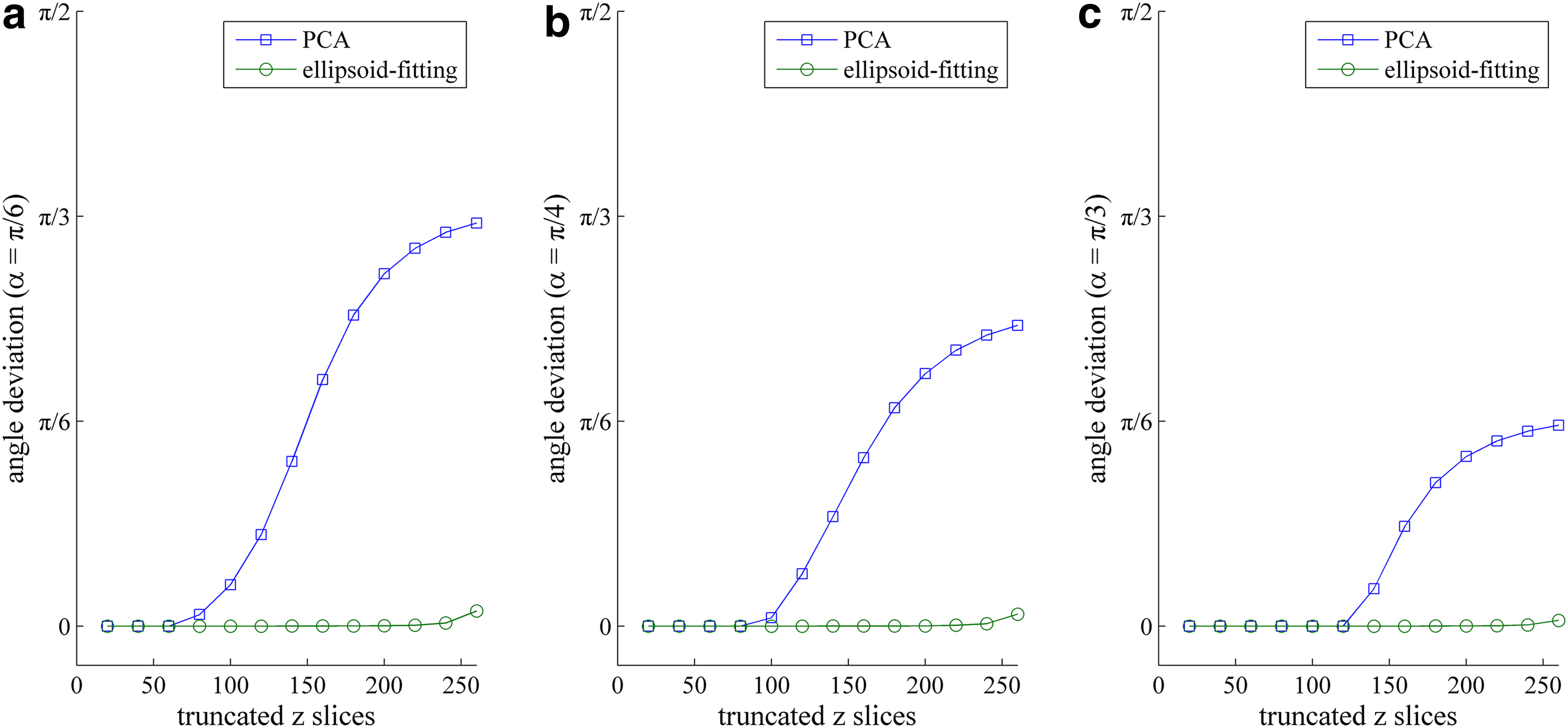
The calculation accuracy of the ellipsoid-fitting method. (a) α = π/6; (b) α = π/4; (c) α = π/3.

5.2. Results on registration

Based on the ellipsoid-fitting method, we registered all the 186 embryos. Figure 11 shows the registration result of 50 WT embryos. For each embryo, we chose the middle time point, during it has two daughters P1 and AB. For the 3D DIC images corresponding to the chosen time point, we selected 11, 16, 21, …, 56 slices from the total 66 ones to show the original embryo. The registered images followed the registration scheme described in Section 4.4 and based on the interpolated DIC images. From the registered DIC image (with size 600 × 600 × 600), we chose 192, 216, 240, …, 408 to show the registration result. In addition, the variation range of intensity in Figure 11 is set to [0,200] to obtain a better observation. In Figure 12, we also show the registered boundaries and the registered fitted ellipsoid.

FIG. 11.

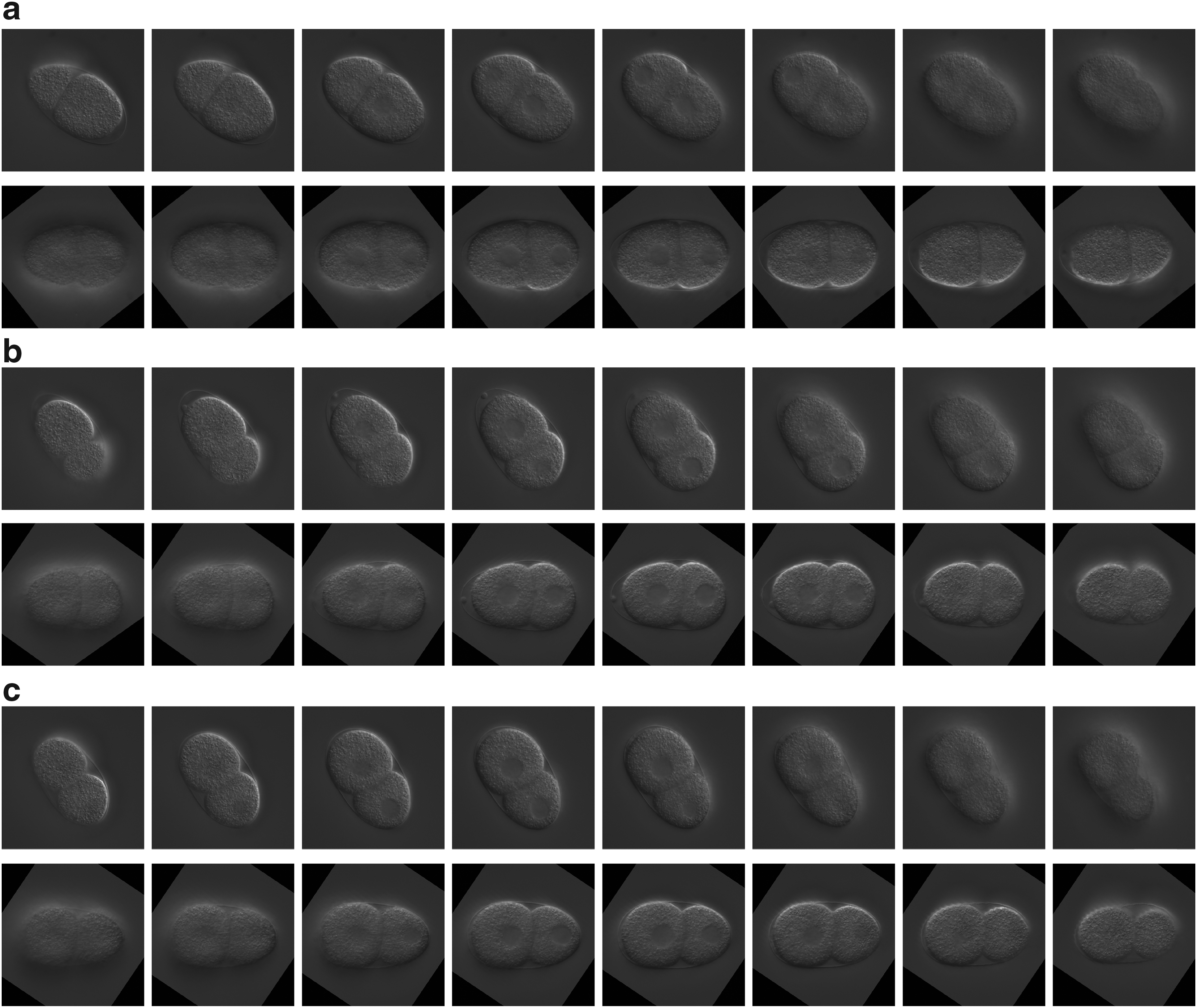
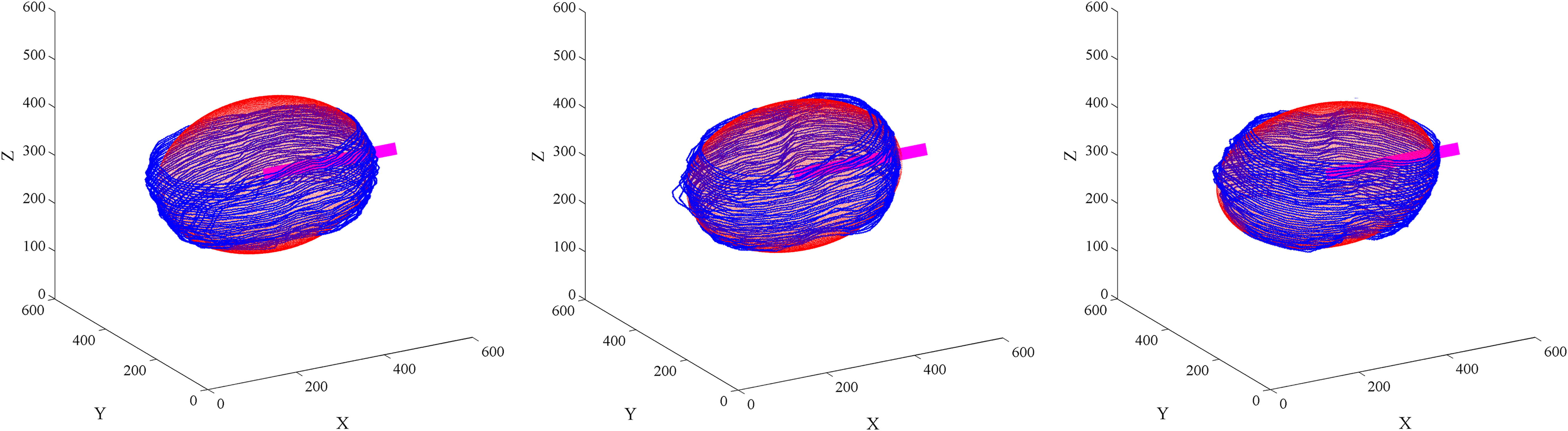
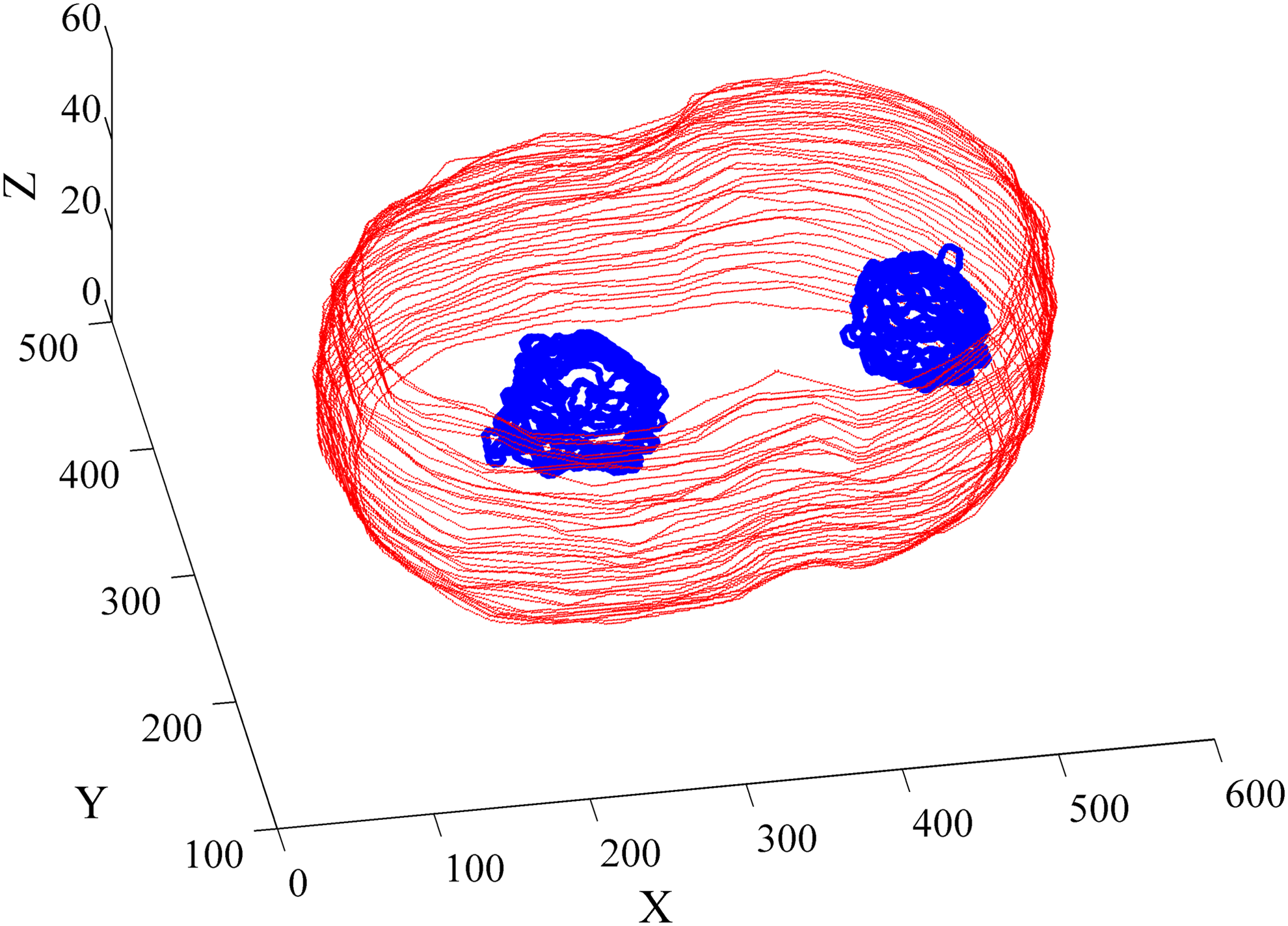
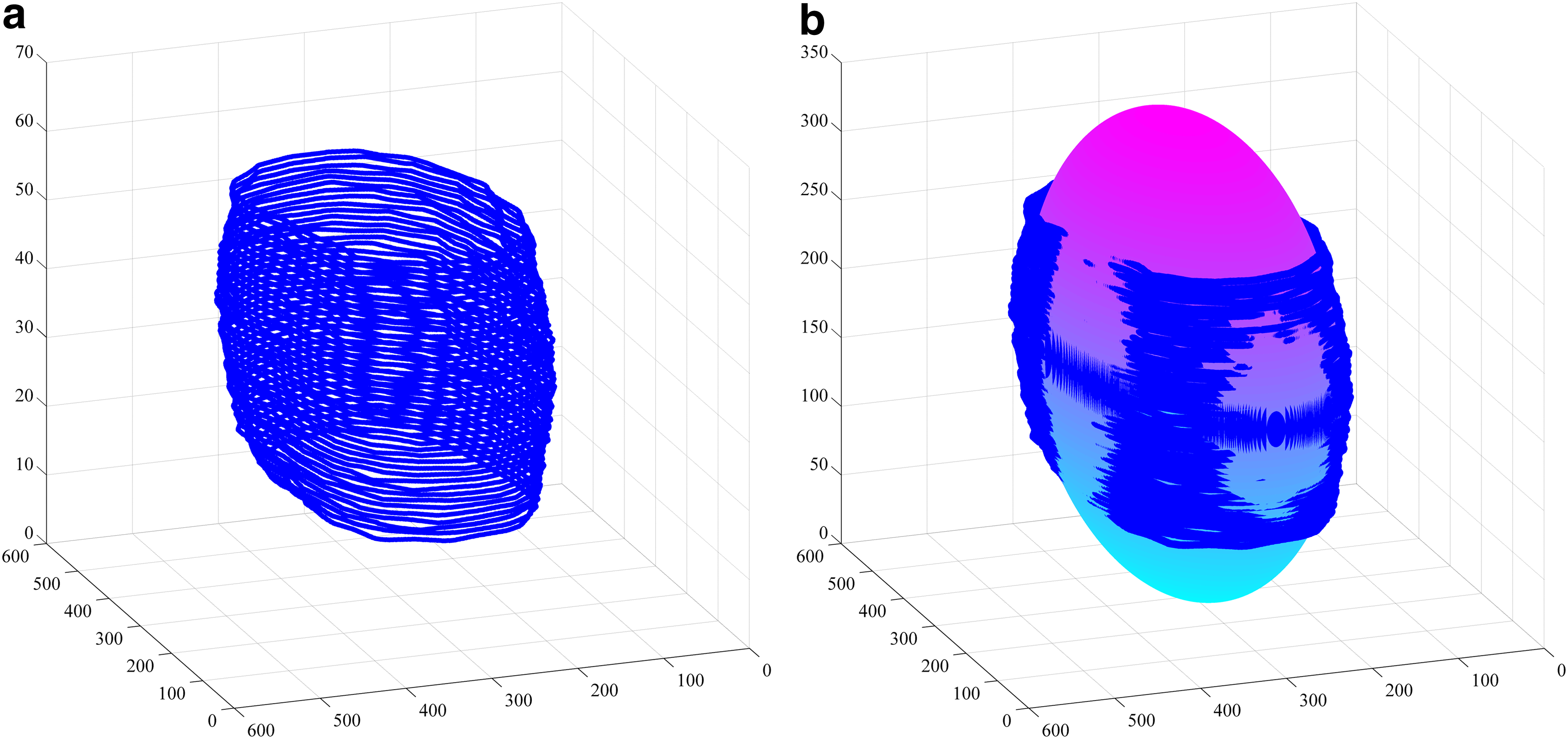
The original images and registered images for WT embryos. The row 1, 3, 5 is original DIC images from three WT embryos, respectively: (a) wt_N2_030203_02, (b) wt_N2_030304_01, (c) wt_N2_030306_01. Each row has 8 slices from a 3D DIC image (with size 600 × 600 × 66) and the slice No. is 16, 21, …, 51. The row 2, 4, 6 is the registered DIC images from the three WT embryos, respectively. Each row has 8 slices from the registered DIC image (with size 600 × 600 × 600) and the slice No. is 216, 240, 264, 288, 312, 336, 360, 384. DIC, differential interference contrast; WT, wild type.

FIG. 12.

The registered segmented boundaries and the registered fitted ellipsoids for the three WT embryos (the same as Fig. 11). In the figure, blue lines are segmented boundaries; red points are fitted ellipsoids; pink bold lines are along the main axes of the ellipsoids. WT, wild type.

6. Conclusion

The emergence of fully automated phenotyping system will allow very large-scale exploratory experiments in functional genomics. Cellular boundary segmentation is a basic and indispensable step in studying morphological embryonic development. This study presented a cellular boundary segmentation algorithm based on the SI and geometric postprocessing techniques. Instead of detecting cellular boundaries themselves, our method focuses on the detection of cytoplasm granules. Experimental results show high accuracy of the method. As we have shown, the proposed method can also be applied to nuclear segmentation with slight modification. As a second-order descriptor of intensity, SI is hardly influenced by the zero-order and first-order variation of intensity, which makes it a desired tool working on images with nonuniform illumination.

As we have demonstrated, using PCA to compute AP axes based on DIC images is ventured. The blur in marginal slices may cause incomplete boundaries, and this will make the calculated AP axes deviate from the correct direction. Using the ellipsoid-fitting method, however, can achieve higher accuracy even when the missing is severe. Based on our experimental results, we recommend using the ellipsoid-fitting method instead of PCA to compute AP axes when the boundaries are similar to ellipsoids.

Footnotes

Acknowledgments

This work was supported in part by the Grant-in Aid for Scientific Research from the Japanese Ministry for Education, Science, Culture and Sports (MEXT) under the Grant No. 18H04747. The work was also supported in part by the Grant-in Aid for Scientific Research from the Huaqiao University under the Grant No. 09HZR13. The authors thank Prof. Nishigawa of Ritsumeikan University, Dr. Onami, Dr. Tohsato, and Dr. Kyoda of RIKEN for their advice in this research.

Author Disclosure Statement

The authors declare that no competing financial interests exist.

References

Adiga

P.U.

, and Chaudhuri

B.B.

2001. An efficient method based on watershed and rule-based merging for segmentation of 3-D histo-pathological images. Pattern Recogn. 34, 1449–1458.

Besl

, and Jain

1986. Invariant surface characteristics for 3D object recognition in range images. Comput. Vis. Graph. Image Proc. 33, 33–80.

Bookstein

F.L.

1979. Fitting conic sections to scattered data. Comput. Graph. Image Proc. 9, 56–71.

Bradley

, and Roth

2007. Adaptive thresholding using the integral image. J. Graphics Tools, 12, 13–21.

Cantzler

, and Fisher

2001. Comparison of HK and SC curvature description methods, 285–291. Proceedings of the 3rd Conference on 3D Digital Imaging and Modeling. IEEE Computer Society Press, Washington, DC.

Dorai

, and Jain

1997. COSMOS—A representation scheme for 3D free-form objects. IEEE Trans. Pattern Anal. Mach. Intell. 19, 1115–1130.

Fitzgibbon

A.W.

, and Fisher

R.B.

1995. A Buyer's guide to conic fitting, 513–522. Proceedings of the 6th British Conference on Machine Vision (BMVC95). BMVA Press, Surrey, United Kingdom.

Fitzgibbon

A.W.

, Pilu

, and Fisher

R.B.

1999. Direct least square fitting of ellipse. IEEE Trans. Pattern Anal. Mach. Intell. 21, 476–480.

Herman

G.T.

, Zheng

, and Bucholtz

C.A.

1992. Shape-based interpolation. IEEE Comput. Graph. and Appl. 12, 69–79.

10.

Huibin

, Morvan

, and Liming

2011. 3D facial expression recognition based on histograms of surface differential quantities, 483–494. Proceedings of the 13th International Conference on Advanced Concepts for Intelligent Vision Systems. Springer, Heidelberg, Germany.

11.

Irshad

, Veillard

, Roux

, et al. 2013. Methods for nuclei detection, segmentation and classification in digital histopathology: A review—Current status and future potential. IEEE Rev. Biomed. Eng. 7, 97–114.

12.

Koenderink

, and Doorn

1992. Surface shape and curvature scales. Image Vis. Comput. 10, 557–564.

13.

Kyoda

, Adachi

, Masuda

, et al. 2013. WDDD: Worm developmental dynamics database. Nucleic Acids Res. 41, 732–737.

14.

, Xu

, Gui

2010. Distance regularized level set evolution and its application to image segmentation. IEEE Trans. Image Proc. 19, 3243–3254.

15.

Lin

G. U

, mesh

, Kathy

, et al. 2003. A hybrid 3D watershed algorithm incorporating gradient cues and object models for automatic segmentation of nuclei in confocal image stacks. Cytometry A, 56A, 23–36.

16.

McInerney

, and Terzopoulos

1996. Deformable models in medical image analysis: A survey. Med. Image Anal. 1, 91–108.

17.

Meijering

2012. Cell segmentation: 50 years down the road. IEEE Trans. Signal Process Magaz. 29, 140–145.

18.

Ning

, LeCun

, Piano

, et al. 2005. Towards automatic phenotyping of developing embryos from videos. IEEE Trans. Image Proc. 14, 1360–1371.

19.

Peet

F.G.

, and Sahota

T.S.

1985. Surface curvature as a measure of image texture. IEEE Trans. Pattern Anal. Mach. Intell. 7, 734–738.

20.

Qingde

, and Griffiths

J.G.

2004. Least squares ellipsoid specific fitting, 335–340. IEEE Conference: Geometric Modeling and Processing (GMP04). IEEE Computer Society, Washington, DC.

21.

Thirion

J.P.

, and Gourdon

1995. Computing the differential characteristics of isointensity surfaces. Comput. Vis. Image Underst. 61, 190–202.

22.

Xing

, and Yang

2016. Robust nucleus/cell detection and segmentation in digital pathology and microscopy images: A comprehensive review. IEEE Rev. Biomed. Eng. 9, 234–263.

23.

Yang

S.H.

, Xu

, and Suzuki

2016. Density index: Extension of the shape index in describing local intensity variations in a 3D Image. J. Comput. Aided Des. Comput. Graph. 28, 1152–1159. [in Chinese.]

24.

Yang

, Han

, and Chen

2017. Automatic segmentation of cellular/nuclear boundaries based on the shape index of image intensity surfaces. The 5th International KES Conference, Invited Session 03(InMed 2017). Vilamoura, Portugal.

25.

Yoshida

, and Näppi

2001. Three-dimensional computer-aided diagnosis scheme for detection of colonic polyps. IEEE Trans. Med. Imaging, 20, 1261–1274.