Efficiently Mining Recurrent Substructures from Protein Three-Dimensional Structure Graphs

Abstract

Studying protein structures is a major asset for understanding the molecular mechanisms of life. The number of publicly available protein structures has increasingly become extremely large. Yet, the classification of a protein structure remains a difficult, costly, and time-consuming task. Exploring spatial information on protein structures can provide important functional and structural insights. In this context, spatial motifs may correspond to relevant fragments, which might be very useful for a better understanding of proteins. In this article, we propose AntMot, a fast algorithm, to find spatial motifs from protein three-dimensional structures by extending the Karp–Miller–Rosenberg repetition finder, originally dedicated to sequences. The extracted motifs, termed ant-motifs, follow an ant-like shape that is composed of a backbone fragment from the primary structure, enriched with spatial refinements. We show that these motifs are biologically sound, and we used them as descriptors in the classification of several benchmark datasets. Experimental results show that our approach presents a trade-off between sequential motifs and subgraph motifs in terms of the number of extracted substructures, while providing a significant enhancement in the classification accuracy over sequential and frequent-subgraph motifs as well as alignment-based approaches.

1. Introduction

The number of proteins in the PDB database (Berman et al., 2000) has more than tripled over the last decade comprising thousands of structures. SCOP (Andreeva et al., 2008), the most reliable database for structural classification, is updated only every 6 months. This is due to the intensive work required in visual inspection. Fast and accurate computational and machine learning classification approaches may offer a considerable boosting to meet the increasing load of data (Muggleton, 2006).

Defining a convenient representation of the internal components of proteins and the existing links between them is a major asset for further computational studies. Proteins have long been processed as strings of characters, where each character represents an amino acid from the primary structure. This linear representation has been used in many bioinformatics and data mining applications (Dominic et al., 1990; Zhang and Zaki, 2006; Saidi et al., 2010). However, such a simplistic encoding of the complex protein structure may fail to provide comprehensive information, especially in some function prediction and classification tasks.

The investigation of the proteins' spatial shape may provide important functional and structural insights (Clark et al., 1991; Cootes et al., 2003). Indeed, protein structures have been interpreted as graphs of amino acids and studied based on graph theory concepts (Borgwardt et al., 2005; Anchuri et al., 2013; Dhifli et al., 2014; Dhifli and Nguifo, 2015; Dhifli et al., 2017; Saha et al., 2017; Mrzic et al., 2018; Sugiyama et al., 2018). In this regard, some works were interested in the study of protein structures based on their graph properties and involved the use of topological classifications as in Bartoli et al. (2007), where it has been shown that proteins can be considered as small-world networks of amino acids. Other works have focused on identifying residues that play the role of hubs that stabilize the structure of the protein (Vallabhajosyula et al., 2009), or on predicting pathways from biological networks (Faust et al., 2010). Another current trend in many recent studies focuses on the subject of discovering motifs from protein structures and using them as features to perform protein classification (Dhifli et al., 2014, 2017; Saha et al., 2017). Our work explores the latter topic. For our purpose, we provide the following comprehensive definitions:

Definition 1 (Motif) In general, a motif consists of a feature that can characterize a given population of objects. This motif may be identified based on given statistical criteria. In our case, a motif is considered to be a significant set of linked amino acids found in a collection of proteins.

Definition 2 (Sequential motif) It consists of a motif whose composing residues are contiguous in the primary structure; that is, it is a subchain extracted from the protein sequence.

Definition 3 (Spatial motif) This consists of a motif whose composing residues are not necessarily contiguous in the primary structure; that is, it may contain linked residues that are far away in the chain but connected in the 3D-space.

In the literature, three-dimensional (3D)-structure-based classification methods mainly use spatial motifs as features to characterize protein groups. Since a protein 3D structure can be seen as a graph of residues, many works have explored the task of frequent-subgraph discovery as a way of finding spatial motifs [MoFa (Borgelt and Berthold, 2002), FFSM (Huan et al., 2003), gSpan (Yan and Han, 2002), Gaston (Nijssen and Kok, 2004), UnSubPatt (Dhifli et al., 2014), FS³ (Saha et al., 2017), etc.]. Some other works focused on the learning process and used the discovered motifs as base learners in boosting algorithms [LEAP (Yan et al., 2008), gboost (Saigo et al., 2009), COM (Jin et al., 2009), and LPGBCMP (Fei and Huan, 2010)].

Although spatial motifs comprise important information that sequential ones fail to provide, the main disadvantage of using subgraphs as features is the high complexity of their extraction due to graph and subgraph isomorphism (Nijssen and Kok, 2004). In addition, the number of extracted subgraphs is expected to be extremely high since proteins are very dense molecules. Hence, the use of such motifs may hinder or even make unfeasible the classification process, especially on real-world large-scale datasets. This article addresses both drawbacks. We propose a novel representation of spatial motifs, which simplifies the existing graph format of motifs while taking into account sequential motifs (SMs) and the links between distant amino acids in the primary structure. We term the discovered spatial motifs ant-motifs (AMs).

2. Methods

2.1. Ant-motif: biological basis

It is known that the tertiary structure of a protein depends on its primary structure (Gille et al., 2000). Thus, two homologous proteins with high-sequence similarity (>80% identical amino acids) will most likely have very similar structures. Usually, SMs have functional meanings, and some of them are easy to recognize (e.g., zinc finger motif) since they are uninterrupted. However, this is not the case with many other motifs, in which the spacing between their elements and even their order can vary considerably (Gille et al., 2000). Moreover, the structure of proteins is more stable than the sequence. Indeed, preserved sequential regions can be lost across the evolutionary time, whereas spatial links persist longer. Hence, it would be judicious to keep the preserved subsequences as bases of motifs (i.e., as backbones) and enrich them with spatial information.

2.2. Shape of an ant-motif

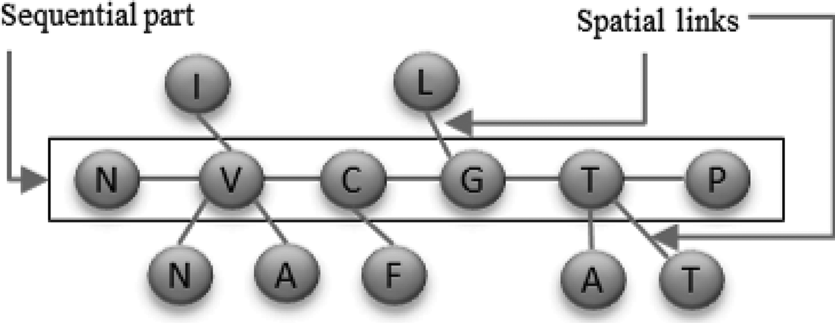
We propose a novel shape of a spatial motif preserving a sequential part from the primary structure and abstracting the spatial information by links with distant residues. This gives the motif an ant-like shape (Figs. 1 and 2 for a real AM example, sampled from our experiments). The sequential part represents the backbone of the motif, which is the largest preserved subsequence, while the spatial links indicate the types of distant residues to which residues of the sequential part are connected. To extract such motifs, we propose an adaptation of the Karp, Miller, and Rosenberg (KMR) algorithm (Karp et al., 1972).

FIG. 1.

Shape of an ant-motif. The sequential part is composed of amino acids from the primary structure, and the spatial links represent their connections to distant residues.

FIG. 2.

An example of an ant-motif sampled from our experiments (in C-type lectin domains [DS4]). The residues ASP (aspartic acid), ALA (alanine), and GLU (glutamic acid) represent the sequential part of the motif. The other ones are distant residues in the 3D structure.

2.3. Karp, Miller, and Rosenberg algorithm

The algorithm of KMR is a method to detect repetitions in a data structure (strings and tables) (Karp et al., 1972). The original version of the KMR algorithm is dedicated to one string, and its complexity is almost linear in the size of the input structure. The original version has been the kernel of other algorithms, and it has been adapted in a parallelized version in Crochemore and Rytter (1991). The KMR algorithm is based on the following notion of equivalence:

Definition 4 (Equivalence in sequences) Two positions i and j in a string S of length m are k-equivalent, we note i E_k j, if and only if the two substrings of length k \documentclass{aastex}\usepackage{amsbsy}\usepackage{amsfonts}\usepackage{amssymb}\usepackage{bm}\usepackage{mathrsfs}\usepackage{pifont}\usepackage{stmaryrd}\usepackage{textcomp}\usepackage{portland, xspace}\usepackage{amsmath, amsxtra}\usepackage{upgreek}\pagestyle{empty}\DeclareMathSizes{10}{9}{7}{6}\begin{document} $$S \left[ {i , i + k - 1} \right]$$ \end{document} and \documentclass{aastex}\usepackage{amsbsy}\usepackage{amsfonts}\usepackage{amssymb}\usepackage{bm}\usepackage{mathrsfs}\usepackage{pifont}\usepackage{stmaryrd}\usepackage{textcomp}\usepackage{portland, xspace}\usepackage{amsmath, amsxtra}\usepackage{upgreek}\pagestyle{empty}\DeclareMathSizes{10}{9}{7}{6}\begin{document} $$S \left[ {j , j + k - 1} \right]$$ \end{document} are identical (Karp et al., 1972).

We also say that the positions i and j belong to the same equivalence class in the level k. An equivalence relation E_k (or a level k), \documentclass{aastex}\usepackage{amsbsy}\usepackage{amsfonts}\usepackage{amssymb}\usepackage{bm}\usepackage{mathrsfs}\usepackage{pifont}\usepackage{stmaryrd}\usepackage{textcomp}\usepackage{portland, xspace}\usepackage{amsmath, amsxtra}\usepackage{upgreek}\pagestyle{empty}\DeclareMathSizes{10}{9}{7}{6}\begin{document} $$1 \le k \le m$$ \end{document} , can be represented by a vector \documentclass{aastex}\usepackage{amsbsy}\usepackage{amsfonts}\usepackage{amssymb}\usepackage{bm}\usepackage{mathrsfs}\usepackage{pifont}\usepackage{stmaryrd}\usepackage{textcomp}\usepackage{portland, xspace}\usepackage{amsmath, amsxtra}\usepackage{upgreek}\pagestyle{empty}\DeclareMathSizes{10}{9}{7}{6}\begin{document} $${V_k} \left[ {1 \ldots m - k + 1} \right]$$ \end{document} , where each component \documentclass{aastex}\usepackage{amsbsy}\usepackage{amsfonts}\usepackage{amssymb}\usepackage{bm}\usepackage{mathrsfs}\usepackage{pifont}\usepackage{stmaryrd}\usepackage{textcomp}\usepackage{portland, xspace}\usepackage{amsmath, amsxtra}\usepackage{upgreek}\pagestyle{empty}\DeclareMathSizes{10}{9}{7}{6}\begin{document} $$V \left[ i \right]$$ \end{document} of this vector, \documentclass{aastex}\usepackage{amsbsy}\usepackage{amsfonts}\usepackage{amssymb}\usepackage{bm}\usepackage{mathrsfs}\usepackage{pifont}\usepackage{stmaryrd}\usepackage{textcomp}\usepackage{portland, xspace}\usepackage{amsmath, amsxtra}\usepackage{upgreek}\pagestyle{empty}\DeclareMathSizes{10}{9}{7}{6}\begin{document} $$1 \le i \le m - k + 1$$ \end{document} , represents the number of the equivalence class to which position i belongs to the equivalence relation E_k. Figure 3 illustrates a case of 2-equivalence between positions \documentclass{aastex}\usepackage{amsbsy}\usepackage{amsfonts}\usepackage{amssymb}\usepackage{bm}\usepackage{mathrsfs}\usepackage{pifont}\usepackage{stmaryrd}\usepackage{textcomp}\usepackage{portland, xspace}\usepackage{amsmath, amsxtra}\usepackage{upgreek}\pagestyle{empty}\DeclareMathSizes{10}{9}{7}{6}\begin{document} $$i = 5$$ \end{document} and \documentclass{aastex}\usepackage{amsbsy}\usepackage{amsfonts}\usepackage{amssymb}\usepackage{bm}\usepackage{mathrsfs}\usepackage{pifont}\usepackage{stmaryrd}\usepackage{textcomp}\usepackage{portland, xspace}\usepackage{amsmath, amsxtra}\usepackage{upgreek}\pagestyle{empty}\DeclareMathSizes{10}{9}{7}{6}\begin{document} $$j = 11$$ \end{document} . We note that it is a repeated substring “NV” of length \documentclass{aastex}\usepackage{amsbsy}\usepackage{amsfonts}\usepackage{amssymb}\usepackage{bm}\usepackage{mathrsfs}\usepackage{pifont}\usepackage{stmaryrd}\usepackage{textcomp}\usepackage{portland, xspace}\usepackage{amsmath, amsxtra}\usepackage{upgreek}\pagestyle{empty}\DeclareMathSizes{10}{9}{7}{6}\begin{document} $$k = 2$$ \end{document} identified in positions \documentclass{aastex}\usepackage{amsbsy}\usepackage{amsfonts}\usepackage{amssymb}\usepackage{bm}\usepackage{mathrsfs}\usepackage{pifont}\usepackage{stmaryrd}\usepackage{textcomp}\usepackage{portland, xspace}\usepackage{amsmath, amsxtra}\usepackage{upgreek}\pagestyle{empty}\DeclareMathSizes{10}{9}{7}{6}\begin{document} $$i = 5$$ \end{document} and \documentclass{aastex}\usepackage{amsbsy}\usepackage{amsfonts}\usepackage{amssymb}\usepackage{bm}\usepackage{mathrsfs}\usepackage{pifont}\usepackage{stmaryrd}\usepackage{textcomp}\usepackage{portland, xspace}\usepackage{amsmath, amsxtra}\usepackage{upgreek}\pagestyle{empty}\DeclareMathSizes{10}{9}{7}{6}\begin{document} $$j = 11$$ \end{document} . This repeated substring is one of equivalence class of the relation E₂ (or level 2).

FIG. 3.

Illustration of 2-equivalence between positions \documentclass{aastex}\usepackage{amsbsy}\usepackage{amsfonts}\usepackage{amssymb}\usepackage{bm}\usepackage{mathrsfs}\usepackage{pifont}\usepackage{stmaryrd}\usepackage{textcomp}\usepackage{portland, xspace}\usepackage{amsmath, amsxtra}\usepackage{upgreek}\pagestyle{empty}\DeclareMathSizes{10}{9}{7}{6}\begin{document} $$i = 5$$ \end{document} and \documentclass{aastex}\usepackage{amsbsy}\usepackage{amsfonts}\usepackage{amssymb}\usepackage{bm}\usepackage{mathrsfs}\usepackage{pifont}\usepackage{stmaryrd}\usepackage{textcomp}\usepackage{portland, xspace}\usepackage{amsmath, amsxtra}\usepackage{upgreek}\pagestyle{empty}\DeclareMathSizes{10}{9}{7}{6}\begin{document} $$j = 11$$ \end{document} .

Given this, KMR provides a characterization of \documentclass{aastex}\usepackage{amsbsy}\usepackage{amsfonts}\usepackage{amssymb}\usepackage{bm}\usepackage{mathrsfs}\usepackage{pifont}\usepackage{stmaryrd}\usepackage{textcomp}\usepackage{portland, xspace}\usepackage{amsmath, amsxtra}\usepackage{upgreek}\pagestyle{empty}\DeclareMathSizes{10}{9}{7}{6}\begin{document} $${E_{k + k \prime }}$$ \end{document} in terms of E_k and \documentclass{aastex}\usepackage{amsbsy}\usepackage{amsfonts}\usepackage{amssymb}\usepackage{bm}\usepackage{mathrsfs}\usepackage{pifont}\usepackage{stmaryrd}\usepackage{textcomp}\usepackage{portland, xspace}\usepackage{amsmath, amsxtra}\usepackage{upgreek}\pagestyle{empty}\DeclareMathSizes{10}{9}{7}{6}\begin{document} $${E_{k \prime }}$$ \end{document} . So that it constructs inductively larger sets E_L by setting \documentclass{aastex}\usepackage{amsbsy}\usepackage{amsfonts}\usepackage{amssymb}\usepackage{bm}\usepackage{mathrsfs}\usepackage{pifont}\usepackage{stmaryrd}\usepackage{textcomp}\usepackage{portland, xspace}\usepackage{amsmath, amsxtra}\usepackage{upgreek}\pagestyle{empty}\DeclareMathSizes{10}{9}{7}{6}\begin{document} $$k \prime = 1$$ \end{document} or \documentclass{aastex}\usepackage{amsbsy}\usepackage{amsfonts}\usepackage{amssymb}\usepackage{bm}\usepackage{mathrsfs}\usepackage{pifont}\usepackage{stmaryrd}\usepackage{textcomp}\usepackage{portland, xspace}\usepackage{amsmath, amsxtra}\usepackage{upgreek}\pagestyle{empty}\DeclareMathSizes{10}{9}{7}{6}\begin{document} $$k \prime = k$$ \end{document} . That is, it increases the length of the substrings by concatenating two substrings from the previous iteration using the following lemma (Karp et al., 1972):

Lemma 1 \documentclass{aastex}\usepackage{amsbsy}\usepackage{amsfonts}\usepackage{amssymb}\usepackage{bm}\usepackage{mathrsfs}\usepackage{pifont}\usepackage{stmaryrd}\usepackage{textcomp}\usepackage{portland, xspace}\usepackage{amsmath, amsxtra}\usepackage{upgreek}\pagestyle{empty}\DeclareMathSizes{10}{9}{7}{6}\begin{document} $$i{E_k}j \; \& \; \left( {i + k} \right) {E_{k \prime }} \left( {j+ k} \right) \Leftrightarrow i{E_{k + k \prime }}j$$ \end{document}

2.4. Extending KMR algorithm to handle ant-motifs

2.4.1. Description

In our case, AM extraction differs from the problem solved by KMR. Indeed, the notion of equivalence in KMR is limited to contiguous elements in a sequence; that is, for a given k there may be no more than one k-equivalence E_k between two positions. We change the definition of the equivalence to be adapted to our needs. Hence, two positions may have many equivalence relations (Fig. 4).

FIG. 4.

Illustration of two 2-equivalences between \documentclass{aastex}\usepackage{amsbsy}\usepackage{amsfonts}\usepackage{amssymb}\usepackage{bm}\usepackage{mathrsfs}\usepackage{pifont}\usepackage{stmaryrd}\usepackage{textcomp}\usepackage{portland, xspace}\usepackage{amsmath, amsxtra}\usepackage{upgreek}\pagestyle{empty}\DeclareMathSizes{10}{9}{7}{6}\begin{document} $$i = 5$$ \end{document} and \documentclass{aastex}\usepackage{amsbsy}\usepackage{amsfonts}\usepackage{amssymb}\usepackage{bm}\usepackage{mathrsfs}\usepackage{pifont}\usepackage{stmaryrd}\usepackage{textcomp}\usepackage{portland, xspace}\usepackage{amsmath, amsxtra}\usepackage{upgreek}\pagestyle{empty}\DeclareMathSizes{10}{9}{7}{6}\begin{document} $$j = 11$$ \end{document} : \documentclass{aastex}\usepackage{amsbsy}\usepackage{amsfonts}\usepackage{amssymb}\usepackage{bm}\usepackage{mathrsfs}\usepackage{pifont}\usepackage{stmaryrd}\usepackage{textcomp}\usepackage{portland, xspace}\usepackage{amsmath, amsxtra}\usepackage{upgreek}\pagestyle{empty}\DeclareMathSizes{10}{9}{7}{6}\begin{document} $$i \;E_2^1\; j \to \left\{ {N , V} \right\} $$ \end{document} and \documentclass{aastex}\usepackage{amsbsy}\usepackage{amsfonts}\usepackage{amssymb}\usepackage{bm}\usepackage{mathrsfs}\usepackage{pifont}\usepackage{stmaryrd}\usepackage{textcomp}\usepackage{portland, xspace}\usepackage{amsmath, amsxtra}\usepackage{upgreek}\pagestyle{empty}\DeclareMathSizes{10}{9}{7}{6}\begin{document} $$i \;E_2^2 \;j \to \left\{ {N , I} \right\} $$ \end{document} .

Definition 5 (Equivalence in graphs) Two positions i and j in a graph G are k-equivalent, we note i \documentclass{aastex}\usepackage{amsbsy}\usepackage{amsfonts}\usepackage{amssymb}\usepackage{bm}\usepackage{mathrsfs}\usepackage{pifont}\usepackage{stmaryrd}\usepackage{textcomp}\usepackage{portland, xspace}\usepackage{amsmath, amsxtra}\usepackage{upgreek}\pagestyle{empty}\DeclareMathSizes{10}{9}{7}{6}\begin{document} $${E_k} j$$ \end{document} , if and only if \documentclass{aastex}\usepackage{amsbsy}\usepackage{amsfonts}\usepackage{amssymb}\usepackage{bm}\usepackage{mathrsfs}\usepackage{pifont}\usepackage{stmaryrd}\usepackage{textcomp}\usepackage{portland, xspace}\usepackage{amsmath, amsxtra}\usepackage{upgreek}\pagestyle{empty}\DeclareMathSizes{10}{9}{7}{6}\begin{document} $$G \left[ i \right] = G \left[ j \right]$$ \end{document} and \documentclass{aastex}\usepackage{amsbsy}\usepackage{amsfonts}\usepackage{amssymb}\usepackage{bm}\usepackage{mathrsfs}\usepackage{pifont}\usepackage{stmaryrd}\usepackage{textcomp}\usepackage{portland, xspace}\usepackage{amsmath, amsxtra}\usepackage{upgreek}\pagestyle{empty}\DeclareMathSizes{10}{9}{7}{6}\begin{document} $$G \left[ i \right]$$ \end{document} is linked to k nodes identical to other k nodes linked to \documentclass{aastex}\usepackage{amsbsy}\usepackage{amsfonts}\usepackage{amssymb}\usepackage{bm}\usepackage{mathrsfs}\usepackage{pifont}\usepackage{stmaryrd}\usepackage{textcomp}\usepackage{portland, xspace}\usepackage{amsmath, amsxtra}\usepackage{upgreek}\pagestyle{empty}\DeclareMathSizes{10}{9}{7}{6}\begin{document} $$G \left[ j \right]$$ \end{document} .

The construction of an AM is performed incrementally throughout the sequential part using Lemma 1 and according to Definition 5. But before applying Lemma 1, all spatial links must be built for each node of the sequential part. When two positions have more than one equivalence relation, it is necessary to merge the resulting motifs. Hence, a larger equivalence is inducted using the following lemma:

Lemma 2 \documentclass{aastex}\usepackage{amsbsy}\usepackage{amsfonts}\usepackage{amssymb}\usepackage{bm}\usepackage{mathrsfs}\usepackage{pifont}\usepackage{stmaryrd}\usepackage{textcomp}\usepackage{portland, xspace}\usepackage{amsmath, amsxtra}\usepackage{upgreek}\pagestyle{empty}\DeclareMathSizes{10}{9}{7}{6}\begin{document} $$iE_{{k_1}}^1j \; \& \; iE_{{k_2}}^2j \; \& \; \ldots \; \& \; iE_{{k_n}1}^nj \leftrightarrow i{E_{ ( ( \sum \nolimits_n^i {{k_i} ) - ( n - 1 ) ) } }}j$$ \end{document}

Proof Let G be a graph, and i and j two positions having n equivalence relations \documentclass{aastex}\usepackage{amsbsy}\usepackage{amsfonts}\usepackage{amssymb}\usepackage{bm}\usepackage{mathrsfs}\usepackage{pifont}\usepackage{stmaryrd}\usepackage{textcomp}\usepackage{portland, xspace}\usepackage{amsmath, amsxtra}\usepackage{upgreek}\pagestyle{empty}\DeclareMathSizes{10}{9}{7}{6}\begin{document} $${E_{{k_1}}} \ldots {E_{{k_n}}}$$ \end{document} . The first equivalence \documentclass{aastex}\usepackage{amsbsy}\usepackage{amsfonts}\usepackage{amssymb}\usepackage{bm}\usepackage{mathrsfs}\usepackage{pifont}\usepackage{stmaryrd}\usepackage{textcomp}\usepackage{portland, xspace}\usepackage{amsmath, amsxtra}\usepackage{upgreek}\pagestyle{empty}\DeclareMathSizes{10}{9}{7}{6}\begin{document} $${E_{{k_1}}}$$ \end{document} allows us to build a motif of size k₁, we note it M₁. Each equivalence relation \documentclass{aastex}\usepackage{amsbsy}\usepackage{amsfonts}\usepackage{amssymb}\usepackage{bm}\usepackage{mathrsfs}\usepackage{pifont}\usepackage{stmaryrd}\usepackage{textcomp}\usepackage{portland, xspace}\usepackage{amsmath, amsxtra}\usepackage{upgreek}\pagestyle{empty}\DeclareMathSizes{10}{9}{7}{6}\begin{document} $${E_{{k_i}}}$$ \end{document} of the remaining \documentclass{aastex}\usepackage{amsbsy}\usepackage{amsfonts}\usepackage{amssymb}\usepackage{bm}\usepackage{mathrsfs}\usepackage{pifont}\usepackage{stmaryrd}\usepackage{textcomp}\usepackage{portland, xspace}\usepackage{amsmath, amsxtra}\usepackage{upgreek}\pagestyle{empty}\DeclareMathSizes{10}{9}{7}{6}\begin{document} $$\left( {n - 1} \right)$$ \end{document} equivalences will increase the size of M₁ by new \documentclass{aastex}\usepackage{amsbsy}\usepackage{amsfonts}\usepackage{amssymb}\usepackage{bm}\usepackage{mathrsfs}\usepackage{pifont}\usepackage{stmaryrd}\usepackage{textcomp}\usepackage{portland, xspace}\usepackage{amsmath, amsxtra}\usepackage{upgreek}\pagestyle{empty}\DeclareMathSizes{10}{9}{7}{6}\begin{document} $${k_i} - 1$$ \end{document} nodes since M₁ already contains the node corresponding to positions i and j. This implies that the final motif will be of size \documentclass{aastex}\usepackage{amsbsy}\usepackage{amsfonts}\usepackage{amssymb}\usepackage{bm}\usepackage{mathrsfs}\usepackage{pifont}\usepackage{stmaryrd}\usepackage{textcomp}\usepackage{portland, xspace}\usepackage{amsmath, amsxtra}\usepackage{upgreek}\pagestyle{empty}\DeclareMathSizes{10}{9}{7}{6}\begin{document} $$( ( \sum {{k_i}} ) - ( n - 1 ) ) , \,i = 1 \ldots n$$ \end{document} . Hence, \documentclass{aastex}\usepackage{amsbsy}\usepackage{amsfonts}\usepackage{amssymb}\usepackage{bm}\usepackage{mathrsfs}\usepackage{pifont}\usepackage{stmaryrd}\usepackage{textcomp}\usepackage{portland, xspace}\usepackage{amsmath, amsxtra}\usepackage{upgreek}\pagestyle{empty}\DeclareMathSizes{10}{9}{7}{6}\begin{document} $$i{E_{ ( ( \sum \nolimits_n^i {{k_i} ) - ( n - 1 ) ) } }}j$$ \end{document} . For example in Figure 4, the two 2-equivalences between \documentclass{aastex}\usepackage{amsbsy}\usepackage{amsfonts}\usepackage{amssymb}\usepackage{bm}\usepackage{mathrsfs}\usepackage{pifont}\usepackage{stmaryrd}\usepackage{textcomp}\usepackage{portland, xspace}\usepackage{amsmath, amsxtra}\usepackage{upgreek}\pagestyle{empty}\DeclareMathSizes{10}{9}{7}{6}\begin{document} $$i = 5$$ \end{document} and \documentclass{aastex}\usepackage{amsbsy}\usepackage{amsfonts}\usepackage{amssymb}\usepackage{bm}\usepackage{mathrsfs}\usepackage{pifont}\usepackage{stmaryrd}\usepackage{textcomp}\usepackage{portland, xspace}\usepackage{amsmath, amsxtra}\usepackage{upgreek}\pagestyle{empty}\DeclareMathSizes{10}{9}{7}{6}\begin{document} $$j = 11$$ \end{document} allow us to induce a new 3-equivalence.

2.4.2. Algorithm and data structures

The general algorithm of our approach is described in Algorithm 1. Graph nodes are ordered according to their positions in the protein primary structure. To avoid processing raw graphs, we parse them into new sequential codes. An index table describing all edges existing in the graph accompanies each graph sequential code. The latter is constructed by inserting between two backbone nodes (two contiguous residues in the primary structure) with indices i and \documentclass{aastex}\usepackage{amsbsy}\usepackage{amsfonts}\usepackage{amssymb}\usepackage{bm}\usepackage{mathrsfs}\usepackage{pifont}\usepackage{stmaryrd}\usepackage{textcomp}\usepackage{portland, xspace}\usepackage{amsmath, amsxtra}\usepackage{upgreek}\pagestyle{empty}\DeclareMathSizes{10}{9}{7}{6}\begin{document} $$i + 1$$ \end{document} all the distant residues with higher indices, having edges with the node i. The node \documentclass{aastex}\usepackage{amsbsy}\usepackage{amsfonts}\usepackage{amssymb}\usepackage{bm}\usepackage{mathrsfs}\usepackage{pifont}\usepackage{stmaryrd}\usepackage{textcomp}\usepackage{portland, xspace}\usepackage{amsmath, amsxtra}\usepackage{upgreek}\pagestyle{empty}\DeclareMathSizes{10}{9}{7}{6}\begin{document} $$i + 1$$ \end{document} and the mentioned distant nodes spatially linked to node i are termed successor nodes. All index tables are concatenated to form a global index table GIT.

Algorithm 1:

AntMot

Require:	GIT
Ensure:	\documentclass{aastex}\usepackage{amsbsy}\usepackage{amsfonts}\usepackage{amssymb}\usepackage{bm}\usepackage{mathrsfs}\usepackage{pifont}\usepackage{stmaryrd}\usepackage{textcomp}\usepackage{portland, xspace}\usepackage{amsmath, amsxtra}\usepackage{upgreek}\pagestyle{empty}\DeclareMathSizes{10}{9}{7}{6}\begin{document} $${ \rm{ \Omega }}$$ \end{document} : set of ant-motifs
1:	Start
2:	\documentclass{aastex}\usepackage{amsbsy}\usepackage{amsfonts}\usepackage{amssymb}\usepackage{bm}\usepackage{mathrsfs}\usepackage{pifont}\usepackage{stmaryrd}\usepackage{textcomp}\usepackage{portland, xspace}\usepackage{amsmath, amsxtra}\usepackage{upgreek}\pagestyle{empty}\DeclareMathSizes{10}{9}{7}{6}\begin{document} $${M_1} \leftarrow$$ \end{document} set of distinct node labels;
3:	\documentclass{aastex}\usepackage{amsbsy}\usepackage{amsfonts}\usepackage{amssymb}\usepackage{bm}\usepackage{mathrsfs}\usepackage{pifont}\usepackage{stmaryrd}\usepackage{textcomp}\usepackage{portland, xspace}\usepackage{amsmath, amsxtra}\usepackage{upgreek}\pagestyle{empty}\DeclareMathSizes{10}{9}{7}{6}\begin{document} $$k \leftarrow 2$$ \end{document} ;
4:	\documentclass{aastex}\usepackage{amsbsy}\usepackage{amsfonts}\usepackage{amssymb}\usepackage{bm}\usepackage{mathrsfs}\usepackage{pifont}\usepackage{stmaryrd}\usepackage{textcomp}\usepackage{portland, xspace}\usepackage{amsmath, amsxtra}\usepackage{upgreek}\pagestyle{empty}\DeclareMathSizes{10}{9}{7}{6}\begin{document} $${ \rm{ \Omega }} \leftarrow {M_1}$$ \end{document} ;
5:	while \documentclass{aastex}\usepackage{amsbsy}\usepackage{amsfonts}\usepackage{amssymb}\usepackage{bm}\usepackage{mathrsfs}\usepackage{pifont}\usepackage{stmaryrd}\usepackage{textcomp}\usepackage{portland, xspace}\usepackage{amsmath, amsxtra}\usepackage{upgreek}\pagestyle{empty}\DeclareMathSizes{10}{9}{7}{6}\begin{document} $$k \ne - 1$$ \end{document} do
6:	construct \documentclass{aastex}\usepackage{amsbsy}\usepackage{amsfonts}\usepackage{amssymb}\usepackage{bm}\usepackage{mathrsfs}\usepackage{pifont}\usepackage{stmaryrd}\usepackage{textcomp}\usepackage{portland, xspace}\usepackage{amsmath, amsxtra}\usepackage{upgreek}\pagestyle{empty}\DeclareMathSizes{10}{9}{7}{6}\begin{document} $$\left\vert {{M_{k - 1}}} \right\vert P$$ \end{document} and \documentclass{aastex}\usepackage{amsbsy}\usepackage{amsfonts}\usepackage{amssymb}\usepackage{bm}\usepackage{mathrsfs}\usepackage{pifont}\usepackage{stmaryrd}\usepackage{textcomp}\usepackage{portland, xspace}\usepackage{amsmath, amsxtra}\usepackage{upgreek}\pagestyle{empty}\DeclareMathSizes{10}{9}{7}{6}\begin{document} $$\left\vert {{M_{k - 1}}} \right\vert Q$$ \end{document} stacks;
7:	for \documentclass{aastex}\usepackage{amsbsy}\usepackage{amsfonts}\usepackage{amssymb}\usepackage{bm}\usepackage{mathrsfs}\usepackage{pifont}\usepackage{stmaryrd}\usepackage{textcomp}\usepackage{portland, xspace}\usepackage{amsmath, amsxtra}\usepackage{upgreek}\pagestyle{empty}\DeclareMathSizes{10}{9}{7}{6}\begin{document} $$i = 1$$ \end{document} to \documentclass{aastex}\usepackage{amsbsy}\usepackage{amsfonts}\usepackage{amssymb}\usepackage{bm}\usepackage{mathrsfs}\usepackage{pifont}\usepackage{stmaryrd}\usepackage{textcomp}\usepackage{portland, xspace}\usepackage{amsmath, amsxtra}\usepackage{upgreek}\pagestyle{empty}\DeclareMathSizes{10}{9}{7}{6}\begin{document} $$\left\vert {GIT} \right\vert$$ \end{document} do
8:	push i in \documentclass{aastex}\usepackage{amsbsy}\usepackage{amsfonts}\usepackage{amssymb}\usepackage{bm}\usepackage{mathrsfs}\usepackage{pifont}\usepackage{stmaryrd}\usepackage{textcomp}\usepackage{portland, xspace}\usepackage{amsmath, amsxtra}\usepackage{upgreek}\pagestyle{empty}\DeclareMathSizes{10}{9}{7}{6}\begin{document} $${P_{GIT \left[ i \right] }}$$ \end{document} ;
9:	for all I in the P stacks do
10:	for all element i in I do
11:	pop i;
12:	\documentclass{aastex}\usepackage{amsbsy}\usepackage{amsfonts}\usepackage{amssymb}\usepackage{bm}\usepackage{mathrsfs}\usepackage{pifont}\usepackage{stmaryrd}\usepackage{textcomp}\usepackage{portland, xspace}\usepackage{amsmath, amsxtra}\usepackage{upgreek}\pagestyle{empty}\DeclareMathSizes{10}{9}{7}{6}\begin{document} $$s \leftarrow$$ \end{document} number of successors of \documentclass{aastex}\usepackage{amsbsy}\usepackage{amsfonts}\usepackage{amssymb}\usepackage{bm}\usepackage{mathrsfs}\usepackage{pifont}\usepackage{stmaryrd}\usepackage{textcomp}\usepackage{portland, xspace}\usepackage{amsmath, amsxtra}\usepackage{upgreek}\pagestyle{empty}\DeclareMathSizes{10}{9}{7}{6}\begin{document} $$GIT \left[ i \right]$$ \end{document}
13:	for \documentclass{aastex}\usepackage{amsbsy}\usepackage{amsfonts}\usepackage{amssymb}\usepackage{bm}\usepackage{mathrsfs}\usepackage{pifont}\usepackage{stmaryrd}\usepackage{textcomp}\usepackage{portland, xspace}\usepackage{amsmath, amsxtra}\usepackage{upgreek}\pagestyle{empty}\DeclareMathSizes{10}{9}{7}{6}\begin{document} $$j = 1$$ \end{document} to s do
14:	push i in \documentclass{aastex}\usepackage{amsbsy}\usepackage{amsfonts}\usepackage{amssymb}\usepackage{bm}\usepackage{mathrsfs}\usepackage{pifont}\usepackage{stmaryrd}\usepackage{textcomp}\usepackage{portland, xspace}\usepackage{amsmath, amsxtra}\usepackage{upgreek}\pagestyle{empty}\DeclareMathSizes{10}{9}{7}{6}\begin{document} $${Q_{GIT \left[ {i + j} \right] }}$$ \end{document} ;
15:	for all O in the Q stacks do
16:	if \documentclass{aastex}\usepackage{amsbsy}\usepackage{amsfonts}\usepackage{amssymb}\usepackage{bm}\usepackage{mathrsfs}\usepackage{pifont}\usepackage{stmaryrd}\usepackage{textcomp}\usepackage{portland, xspace}\usepackage{amsmath, amsxtra}\usepackage{upgreek}\pagestyle{empty}\DeclareMathSizes{10}{9}{7}{6}\begin{document} $$\left\vert O \right\vert \ge 2$$ \end{document} then
17:	construct a motif based on Lemma 1;
18:	if \documentclass{aastex}\usepackage{amsbsy}\usepackage{amsfonts}\usepackage{amssymb}\usepackage{bm}\usepackage{mathrsfs}\usepackage{pifont}\usepackage{stmaryrd}\usepackage{textcomp}\usepackage{portland, xspace}\usepackage{amsmath, amsxtra}\usepackage{upgreek}\pagestyle{empty}\DeclareMathSizes{10}{9}{7}{6}\begin{document} $$k = 2$$ \end{document} then
19:	merge motifs satisfying Lemma 2;
20:	if \documentclass{aastex}\usepackage{amsbsy}\usepackage{amsfonts}\usepackage{amssymb}\usepackage{bm}\usepackage{mathrsfs}\usepackage{pifont}\usepackage{stmaryrd}\usepackage{textcomp}\usepackage{portland, xspace}\usepackage{amsmath, amsxtra}\usepackage{upgreek}\pagestyle{empty}\DeclareMathSizes{10}{9}{7}{6}\begin{document} $${M_k} = \emptyset$$ \end{document} then
21:	\documentclass{aastex}\usepackage{amsbsy}\usepackage{amsfonts}\usepackage{amssymb}\usepackage{bm}\usepackage{mathrsfs}\usepackage{pifont}\usepackage{stmaryrd}\usepackage{textcomp}\usepackage{portland, xspace}\usepackage{amsmath, amsxtra}\usepackage{upgreek}\pagestyle{empty}\DeclareMathSizes{10}{9}{7}{6}\begin{document} $$k \leftarrow - 1$$ \end{document} ;
22:	Else
23:	\documentclass{aastex}\usepackage{amsbsy}\usepackage{amsfonts}\usepackage{amssymb}\usepackage{bm}\usepackage{mathrsfs}\usepackage{pifont}\usepackage{stmaryrd}\usepackage{textcomp}\usepackage{portland, xspace}\usepackage{amsmath, amsxtra}\usepackage{upgreek}\pagestyle{empty}\DeclareMathSizes{10}{9}{7}{6}\begin{document} $${ \rm{ \Omega }} \leftarrow { \rm{ \Omega }} \cup {M_k}$$ \end{document} ;
24:	remove redundant motifs from \documentclass{aastex}\usepackage{amsbsy}\usepackage{amsfonts}\usepackage{amssymb}\usepackage{bm}\usepackage{mathrsfs}\usepackage{pifont}\usepackage{stmaryrd}\usepackage{textcomp}\usepackage{portland, xspace}\usepackage{amsmath, amsxtra}\usepackage{upgreek}\pagestyle{empty}\DeclareMathSizes{10}{9}{7}{6}\begin{document} $${ \rm{ \Omega }}$$ \end{document} ;
25:	End

Motifs are incrementally built using Lemma 1 and Lemma 2. In each level, we adopt a stack-based implementation to look for common positions allowing the concatenation or the merge of motifs of low levels. In each level, two stack families P and Q are used. The number of stacks in each family is the number of motifs extracted in the previous level.

3. Experiments

3.1. Aims

The experimental study is composed of two parts. We are interested in evaluating the significance of our motifs in protein classification and the runtime of their extraction. To study the first aspect, we perform multiple motif-based classification experiments on various benchmark datasets. We study the effect of three types of motifs on the classification performance, namely SM, frequent-subgraph motifs (FSMs), and AMs. To study the second aspect, we compare our algorithm AntMot with state-of-the-art methods of frequent-subgraph extraction in terms of runtime. We study the behavior of both methods when increasing the amount of data and varying the frequency threshold of motifs. For both criteria (i.e., significance and runtime), the number of motifs is an influencing factor that must be discussed. We further compare AM-based classification with other classification approaches.

3.2. Datasets

We use the same six benchmark datasets of protein structures that have previously been used in Fei and Huan (2010) and Dhifli et al. (2014). In each dataset, positive proteins are sampled from a selected protein family, whereas negative proteins are randomly sampled from the Protein Data Bank (Berman et al., 2000). A detailed description of the data collection process can be found in Fei and Huan (2010) and Jin et al. (2009). Table 1 summarizes the characteristics of the six datasets: protein family ID in SCOP database (Andreeva et al., 2008), description of the protein family, number of positive and negative samples. The selected positive protein families are vertebrate phospholipase A2, G-protein family, C1-set domains, C-type lectin domains, and protein kinases, catalytic subunits.

Table 1.

Experimental Datasets

Dataset	SCOP ID	Family name	Pos	Neg
DS1	48623	Vertebrate phospholipase A2	29	29
DS2	52592	G-proteins	33	33
DS3	48942	C1 set domains	38	38
DS4	56437	C-type lectin domains	38	38
DS5	56251	Subunits of the proteasome core particle	35	35
DS6	88854	Protein kinases, catalytic subunits	41	41

Neg, number of negative proteins; Pos, number of positive proteins; SCOP ID, identifier of protein family in SCOP.

3.3. Settings

Our algorithm, AntMot, is implemented in java. It allows extracting AM as well as SM from protein primary structures. Since the existing algorithms of frequent-subgraph discovery are supposed to extract the same number of motifs, we choose to use Gaston (Nijssen and Kok, 2004), which is known to be the fastest approach for extracting FSM. We use a java implementation for both AntMot and Gaston (available at https://www2.informatik.uni-erlangen.de/EN/research/ParSeMiS/index.html). Experiments were conducted on a 3 Ghz quad core CPU. Gaston is memory greedy and required, in some tests, tens of GBs of RAM; whereas 1 GB was largely enough for AntMot.

3.3.1. Graph building settings

Proteins are parsed into graphs, where nodes represent amino acid residues and are labeled with the respective amino acid type. Two nodes u and v are linked by an edge \documentclass{aastex}\usepackage{amsbsy}\usepackage{amsfonts}\usepackage{amssymb}\usepackage{bm}\usepackage{mathrsfs}\usepackage{pifont}\usepackage{stmaryrd}\usepackage{textcomp}\usepackage{portland, xspace}\usepackage{amsmath, amsxtra}\usepackage{upgreek}\pagestyle{empty}\DeclareMathSizes{10}{9}{7}{6}\begin{document} $$e \left( {u , v} \right) = 1$$ \end{document} if the Euclidean distance between their two \documentclass{aastex}\usepackage{amsbsy}\usepackage{amsfonts}\usepackage{amssymb}\usepackage{bm}\usepackage{mathrsfs}\usepackage{pifont}\usepackage{stmaryrd}\usepackage{textcomp}\usepackage{portland, xspace}\usepackage{amsmath, amsxtra}\usepackage{upgreek}\pagestyle{empty}\DeclareMathSizes{10}{9}{7}{6}\begin{document} $${C_ \alpha }$$ \end{document} atoms \documentclass{aastex}\usepackage{amsbsy}\usepackage{amsfonts}\usepackage{amssymb}\usepackage{bm}\usepackage{mathrsfs}\usepackage{pifont}\usepackage{stmaryrd}\usepackage{textcomp}\usepackage{portland, xspace}\usepackage{amsmath, amsxtra}\usepackage{upgreek}\pagestyle{empty}\DeclareMathSizes{10}{9}{7}{6}\begin{document} $${ \rm{ \Delta }} \left( {{C_ \alpha } \left( u \right) , {C_ \alpha } \left( v \right) } \right)$$ \end{document} is below a threshold \documentclass{aastex}\usepackage{amsbsy}\usepackage{amsfonts}\usepackage{amssymb}\usepackage{bm}\usepackage{mathrsfs}\usepackage{pifont}\usepackage{stmaryrd}\usepackage{textcomp}\usepackage{portland, xspace}\usepackage{amsmath, amsxtra}\usepackage{upgreek}\pagestyle{empty}\DeclareMathSizes{10}{9}{7}{6}\begin{document} $$\delta$$ \end{document} . In our experiments, we use \documentclass{aastex}\usepackage{amsbsy}\usepackage{amsfonts}\usepackage{amssymb}\usepackage{bm}\usepackage{mathrsfs}\usepackage{pifont}\usepackage{stmaryrd}\usepackage{textcomp}\usepackage{portland, xspace}\usepackage{amsmath, amsxtra}\usepackage{upgreek}\pagestyle{empty}\DeclareMathSizes{10}{9}{7}{6}\begin{document} $$\delta = 7$$ \end{document} Å} as in Fei and Huan (2010).

3.3.2. Classification settings

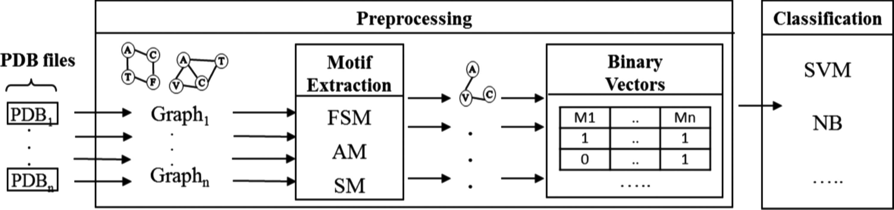
The classification process is illustrated in Figure 5. Input data are protein structures in PDB format (Berman et al., 2000). First, proteins are parsed into graphs. Then, a motif extraction method is used to find frequent motifs. Each protein is encoded into a binary feature vector indexed by the extracted motifs with values indicating the presence (1) or the absence (0) of the related motif in the considered protein. Finally, we apply a classifier on the binary data. We use five replicates of 5-cross-validation as evaluation technique. AMs, SMs, and FSMs are generated with a minimum frequency threshold of 0.3 and motif sizes between 3 and 7 nodes. To show that the classification results are not biased by the classifier, we use two different classifiers, namely support vector machine (SVM) and naïve bayes (NB), from the workbench Weka (Witten and Frank, 2005) with default parameters.

FIG. 5.

Classification process. First, proteins are parsed into graphs. Then, motifs are extracted and used as features to encode proteins into binary vectors with values indicating the presence (1) or absence (0) of the related motif. Finally, binary vectors are used as input for classifiers.

3.3.3. Runtime test settings

To study the variation of runtime with a larger amount of data, we gathered all distinct graphs of the six datasets to form a single one of 392 graphs. We run AntMot and Gaston on this dataset to, respectively, extract AM and FSM while varying the minimum frequency threshold \documentclass{aastex}\usepackage{amsbsy}\usepackage{amsfonts}\usepackage{amssymb}\usepackage{bm}\usepackage{mathrsfs}\usepackage{pifont}\usepackage{stmaryrd}\usepackage{textcomp}\usepackage{portland, xspace}\usepackage{amsmath, amsxtra}\usepackage{upgreek}\pagestyle{empty}\DeclareMathSizes{10}{9}{7}{6}\begin{document} $$\tau$$ \end{document} from 0.1 to 1, without constraints on the size of motifs.

4. Results and Discussion

4.1. Comparing motif extraction methods

4.1.1. Evaluating the significance of motifs in classification

We report the classification accuracy, the sensitivity, and the specificity of the combination of SVM and NB with the motif extraction approaches SM, AM, and FSM. The experimental results are shown in Table 2 and Figure 6. We notice that Gaston generates an extremely large number of motifs, especially with DS1 and DS6. This illustrates the case of information overload (Hasan and Zaki, 2009), a real obstacle for any further motif-based analysis. Indeed, this explains why the classification performance was negatively affected compared with the other approaches. FSM performed better with SVM than NB. This is explained by the selective ability of SVM. Exceptionally, in the case of DS1 using only SM allowed us to almost classify all the instances (except one) correctly. Adding structural motifs to AM or FSM did not help resolve the misclassification.

FIG. 6.

Average accuracy results using SM, AM, and FSM as features and NB (a) and SVM (b) as classifiers. AM, ant-motifs; FSM, frequent-subgraph motifs; NB, naïve bayes; SM, sequential motifs; SVM, support vector machine.

Table 2.

Number of Motifs with Minimum Frequency Threshold of 30% and Having Between 3 and 7 Nodes

	No. of discovered motifs
Method	DS1	DS2	DS3	DS4	DS5	DS6
SM	23	11	54	12	15	26
AM	1994	2007	2132	1366	1152	1725
FSM	1,081,501	680,525	196,867	80,290	764,356	951,657

AM, ant-motifs; FSM, frequent-subgraph motifs; SM, sequential motifs.

Overall, SM presented a reduced number of motifs. Yet, they allowed a better classification performance than FSM in most cases. This highlights the fact that the gain in spatial information offered by FSM is promptly lost due to the curse of dimensionality effect (Hasan and Zaki, 2009) caused by their very large number. The number of motifs of AM presents a trade-off between that of SM and FSM. Figure 6 shows that overall AM provides the best classification performance with both SVM and NB, compared with SM and FSM. This is due to the AM structure that incorporates sequential regions from the primary structure enriched by spatial links in a simple and efficient way that allows us to overcome the problem of information overload and consequently the curse of dimensionality (see Fig. 2 for a real example of an AM). To better understand the classification accuracy differences, we plot the average sensitivity and specificity for all methods. Figure 7 shows the obtained results. It is clear that overall AM provides a better trade-off between sensitivity and specificity than both FSM and SM on the six datasets.

FIG. 7.

Average sensitivity (a) and specificity (b) results using SM, AM, and FSM as features and SVM and NB as classifiers.

4.1.2. Runtime evaluation

Figure 8a shows that the runtime for both AntMot and Gaston is inversely proportional to \documentclass{aastex}\usepackage{amsbsy}\usepackage{amsfonts}\usepackage{amssymb}\usepackage{bm}\usepackage{mathrsfs}\usepackage{pifont}\usepackage{stmaryrd}\usepackage{textcomp}\usepackage{portland, xspace}\usepackage{amsmath, amsxtra}\usepackage{upgreek}\pagestyle{empty}\DeclareMathSizes{10}{9}{7}{6}\begin{document} $$\tau$$ \end{document} . Indeed, a lower \documentclass{aastex}\usepackage{amsbsy}\usepackage{amsfonts}\usepackage{amssymb}\usepackage{bm}\usepackage{mathrsfs}\usepackage{pifont}\usepackage{stmaryrd}\usepackage{textcomp}\usepackage{portland, xspace}\usepackage{amsmath, amsxtra}\usepackage{upgreek}\pagestyle{empty}\DeclareMathSizes{10}{9}{7}{6}\begin{document} $$\tau$$ \end{document} allows extracting more motifs (Fig. 8b) and, hence, too much computation is required. Although Gaston is slightly faster than AntMot for higher \documentclass{aastex}\usepackage{amsbsy}\usepackage{amsfonts}\usepackage{amssymb}\usepackage{bm}\usepackage{mathrsfs}\usepackage{pifont}\usepackage{stmaryrd}\usepackage{textcomp}\usepackage{portland, xspace}\usepackage{amsmath, amsxtra}\usepackage{upgreek}\pagestyle{empty}\DeclareMathSizes{10}{9}{7}{6}\begin{document} $$\tau$$ \end{document} , the latter scales remarkably better to lower \documentclass{aastex}\usepackage{amsbsy}\usepackage{amsfonts}\usepackage{amssymb}\usepackage{bm}\usepackage{mathrsfs}\usepackage{pifont}\usepackage{stmaryrd}\usepackage{textcomp}\usepackage{portland, xspace}\usepackage{amsmath, amsxtra}\usepackage{upgreek}\pagestyle{empty}\DeclareMathSizes{10}{9}{7}{6}\begin{document} $$\tau$$ \end{document} . Indeed, AntMot runtime increases almost linearly with an approximate gradient of 1.75, whereas Gaston runtime increases exponentially to reach >3 days with \documentclass{aastex}\usepackage{amsbsy}\usepackage{amsfonts}\usepackage{amssymb}\usepackage{bm}\usepackage{mathrsfs}\usepackage{pifont}\usepackage{stmaryrd}\usepackage{textcomp}\usepackage{portland, xspace}\usepackage{amsmath, amsxtra}\usepackage{upgreek}\pagestyle{empty}\DeclareMathSizes{10}{9}{7}{6}\begin{document} $$\tau = 0.1$$ \end{document} . The runtime tendency of both algorithms is consistent with the evolution of the number of motifs extracted by each of them. Indeed, the difference in runtime between the two algorithms derives from the huge difference in the number of discovered motifs.

FIG. 8.

Evolution of runtime (a) and number of motifs (b) depending on the minimum frequency threshold.

4.2. Comparison with other classification approaches

We compare our approach with multiple state-of-the-art protein classification approaches, namely sequence alignment-based classification [using Blast (Altschul et al., 1990)], structural alignment-based classification [using Sheba (Jung and Lee, 2000) and FatCat (Ye and Godzik, 2003)], and subgraph-based classification [using GAIA (Jin et al., 2010), LPGBCMP (Fei and Huan, 2010), and D&D (Zhu et al., 2012)]. For sequence and structural alignment-based classification, we align each protein against all the rest of the dataset. We assign to the query protein the function of the reference protein with the best hit score. For the substructure-based approaches, all the selected approaches are mainly for mining discriminative subgraphs. LPGBCMP is used with \documentclass{aastex}\usepackage{amsbsy}\usepackage{amsfonts}\usepackage{amssymb}\usepackage{bm}\usepackage{mathrsfs}\usepackage{pifont}\usepackage{stmaryrd}\usepackage{textcomp}\usepackage{portland, xspace}\usepackage{amsmath, amsxtra}\usepackage{upgreek}\pagestyle{empty}\DeclareMathSizes{10}{9}{7}{6}\begin{document} $$ma{x_{var}} = 1$$ \end{document} and \documentclass{aastex}\usepackage{amsbsy}\usepackage{amsfonts}\usepackage{amssymb}\usepackage{bm}\usepackage{mathrsfs}\usepackage{pifont}\usepackage{stmaryrd}\usepackage{textcomp}\usepackage{portland, xspace}\usepackage{amsmath, amsxtra}\usepackage{upgreek}\pagestyle{empty}\DeclareMathSizes{10}{9}{7}{6}\begin{document} $$d = 0.25$$ \end{document} , respectively, for feature consistency map building and overlapping. In Fei and Huan (2010), LPGBCMP outperformed several other approaches from the literature, including LEAP (Yan et al., 2008), gPLS (Saigo et al., 2008), and COM (Jin et al., 2009), on the classification of the same six benchmark datasets. GAIA showed in Jin et al. (2010) that it outperformed other state-of-the-art approaches, namely COM and graphSig (Ranu and Singh, 2009). D&D have shown in Zhu et al. (2012) that it also outperformed COM and graphSig, and that it is highly competitive to GAIA.

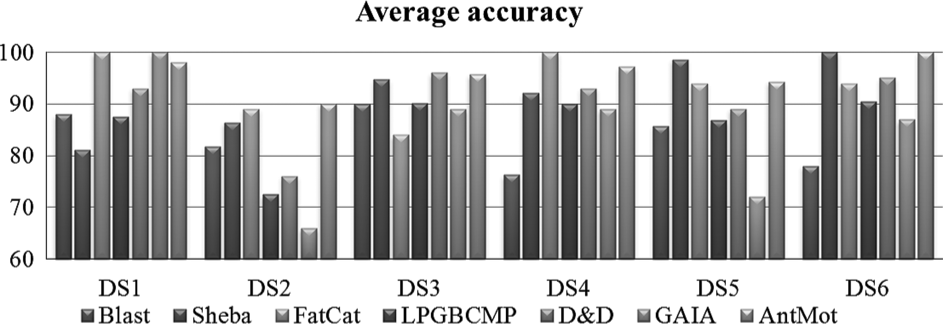
For all these subgraph-based approaches, the discovered subgraphs are considered as features for encoding each protein into a binary vector with 0 and 1, respectively, for the absence or the presence of the subgraph in the protein structure. For our approach AntMot, we used 30% as minimum frequency threshold and SVM as classifier. The Figure 9 shows the obtained results.

FIG. 9.

Comparison of the classification accuracy of AM-based classification with state-of-the-art approaches.

On average, the structural alignment-based approaches FatCat and Sheba outperformed Blast and all the subgraph-based approaches, namely LPGBCMP, D&D, and GAIA. Indeed, FatCat scored better than all these methods with DS1, DS2, and DS4, and Sheba scored best with the two last datasets. On average, all the other approaches scored better than Blast. This shows that the spatial information constitutes an important asset for protein classification by emphasizing structural properties that the primary sequence alone does not provide. For the subgraph-based approaches, D&D scored better than LPGBCMP and GAIA on all cases except with DS1 where GAIA scored best. FatCat presents the most competitive approach to AntMot, followed by Sheba, then D&D. However, on average, AntMot outperformed all the other classification approaches. This is because AntMot presents a simpler yet efficient representation of spatial motifs that at the same time (1) incorporates connections between distant residues that are missing in SM, and (2) allows us to consider spatial links while overcoming the information overload trap that overburden subgraph motifs.

5. Conclusion

In this article, we proposed a novel approach to extract spatial motifs with an ant-like shape that we termed AM. AM allows us to incorporate spatial links that are missing in SM while avoiding the problem of information overload that overburden subgraph motifs. We showed through an evaluation on several benchmark datasets that these motifs are computationally significant, and that they present a better alternative to both sequential and subgraph motifs. Experimental results show that our approach allows a more accurate protein classification than multiple state-of-the-art classification systems, including sequence and structure alignment-based classification, and subgraph-based classification approaches. As future work, we plan to extend our proposed method to take into account the substitution between amino acid residues as in Saidi et al. (2010) and Dhifli et al. (2014).

Footnotes

Author Disclosure Statement

The authors declare that no competing financial interests exist.

References

Altschul

, Gish

, Miller

, et al. 1990. Basic local alignment search tool. J Mol Biol, 215, 403–410.

Anchuri

, Zaki

M.J.

, Barkol

, et al. 2013. Approximate graph mining with label costs. Presented at the Proceedings of the 19th ACM SIGKDD International Conference on Knowledge Discovery and Data Mining, KDD’13, Chicago, IL, USA. pp. 518–526.

Andreeva

, Howorth

, Chandonia

J.-M.

, et al. 2008. Data growth and its impact on the scop database: New developments. Nucleic Acids Res, 36, D419–D425.

Bartoli

, Fariselli

, and Casadio

2007. The effect of backbone on the small-world properties of protein contact maps. Phys Biol, 4, L1–L5.

Berman

H.M.

, Westbrook

J.D.

, Feng

, et al. 2000. The protein data bank. Nucleic Acids Res, 28, 235–242.

Borgelt

, and Berthold

M.R.

2002. Mining molecular fragments: Finding relevant substructures of molecules. Presented at the Proceedings of the 2002 IEEE International Conference on Data Mining, ICDM’02, Maebashi City, Japan. Volume 2, pp. 51–58.

Borgwardt

K.M.

, Ong

C.S.

, Schönauer

, et al. 2005. Protein function prediction via graph kernels. Bioinformatics, 21, 47–56.

Clark

D.A.

, Rawlings

C.J.

, Baron

G.J.

, et al. 1990. Knowledge-based orchestration of protein sequence analysis and knowledge acquisition for protein structure prediction. Presented at the AAAI Spring Symposium, Stanford University, Stanford, CA, USA. pp. 28–32.

Clark

D.A.

, Shirazi

, and Rawlings

C.J.

1991. Protein topology prediction through constraint-based search and the evaluation of topological folding rules. Protein Eng, 4, 751–760.

10.

Cootes

A.P.

, Muggleton

S.H.

, and Sternberg

M.J.E.

2003. The automatic discovery of structural principles describing protein fold space. J Mol Biol, 330, 839–850.

11.

Crochemore

, and Rytter

1991. Usefulness of the Karp-Miller-Rosenberg algorithm in parallel computations on strings and arrays. Theor Comput Sci, 88, 59–82.

12.

Dhifli

, Aridhi

, and Nguifo

E.M.

2017. Mr-simlab: Scalable subgraph selection with label similarity for big data. Inf Syst, 69, 155–163.

13.

Dhifli

, and Mephu Nguifo

2015. Motif discovery in protein 3D-structures using graph mining techniques, 167–189. In Pattern Recognition in Computational Molecular Biology: Techniques and Approaches. John Wiley & Sons, Hoboken, NJ, USA.

14.

Dhifli

, Saidi

, and Nguifo

E.M.

2014. Smoothing 3D protein structure motifs through graph mining and amino-acids similarities. J Comput Biol, 21, 162–172.

15.

Faust

, Dupont

, Callut

, et al. 2010. Pathway discovery in metabolic networks by subgraph extraction. Bioinformatics, 26, 1211–1218.

16.

Fei

, and Huan

2010. Boosting with structure information in the functional space: An application to graph classification. Presented at the Proceedings of the 16th ACM SIGKDD International Conference on Knowledge Discovery and Data Mining, KDD’10, Washington, DC, USA. pp. 643–652.

17.

Gille

, Goede

, Preissner

, et al. 2000. Conservation of substructures in proteins: Interfaces of secondary structural elements in proteasomal subunits. J Mol Biol, 299, 1147–1154.

18.

Hasan

M.A.

, and Zaki

M.J.

2009. Output space sampling for graph patterns. Proc VLDB Endowment, 2, 730–741.

19.

Huan

, Wang

, and Prins

2003. Efficient mining of frequent subgraphs in the presence of isomorphism. Presented at the Proceedings of the 2003 IEEE International Conference on Data Mining, ICDM’03, Melbourne, FL, USA. pp. 549–552.

20.

Jin

, Young

, and Wang

2009. Graph classification based on pattern co-occurrence. Presented at the Proceedings of the 18th ACM Conference on Information and Knowledge Management, CIKM’09, Hong Kong, China. pp. 573–582.

21.

Jin

, Young

, and Wang

2010. GAIA: Graph classification using evolutionary computation. Presented at the Proceedings of the 2010 ACM SIGMOD International Conference on Management of Data, SIGMOD’10, Indianapolis, IN, USA. pp. 879–890.

22.

Jung

, and Lee

2000. Protein structure alignment using environmental profiles. Protein Eng, 13, 535–543.

23.

Karp

R.M.

, Miller

R.E.

, and Rosenberg

A.L.

1972. Rapid identification of repeated patterns in strings, trees and arrays. Presented at the Proceedings of the Fourth Annual ACM Symposium on Theory of Computing, STOC’72, Denver, CO, USA. pp. 125–136.

24.

Mrzic

, Meysman

, Bittremieux

, et al. 2018. Grasping frequent subgraph mining for bioinformatics applications. BioData Min, 11, 20.

25.

Muggleton

S.H.

2006. 2020 computing: Exceeding human limits. Nature, 440, 409–410.

26.

Nijssen

, and Kok

J.N.

2004. A quickstart in frequent structure mining can make a difference. Presented at the Proceedings of the Tenth ACM SIGKDD International Conference on Knowledge Discovery and Data Mining, KDD’04, Seattle, WA, USA. pp. 647–652.

27.

Ranu

, and Singh

A.K.

2009. Graphsig: A scalable approach to mining significant subgraphs in large graph databases. Presented at the IEEE 25th International Conference on Data Engineering, ICDE’09, Shanghai, China. 844–855.

28.

Saha

T.K.

, Katebi

, Dhifli

, et al. 2017. Discovery of functional motifs from the interface region of oligomeric proteins using frequent subgraph mining. IEEE/ACM Trans Comput Biol Bioinform. In press. DOI: 10.1109/TCBB.2017.2756879.

29.

Saidi

, Maddouri

, and Mephu Nguifo

2010. Protein sequences classification by means of feature extraction with substitution matrices. BMC Bioinformatics, 11, 175.

30.

Saigo

, Krämer

, and Tsuda

2008. Partial least squares regression for graph mining. Presented at the Proceedings of the 14th ACM SIGKDD International Conference on Knowledge Discovery and Data Mining, KDD’08, Las Vegas, NV, USA. pp. 578–586.

31.

Saigo

, Nowozin

, Kadowaki

, et al. 2009. A mathematical programming approach to graph classification and regression. Mach Learn, 75, 69–89.

32.

Sugiyama

, Ghisu

M.E.

, Llinares-López

, et al. 2018. graphkernels: R and python packages for graph comparison. Bioinformatics, 34, 530–532.

33.

Vallabhajosyula

R.R.

, Chakravarti

, Lutfeali

, et al. 2009. Identifying hubs in protein interaction networks. PLoS One, 4, e5344.

34.

Witten

I.H.

, and Frank

2005. Data Mining: Practical Machine Learning Tools and Techniques. Morgan Kaufmann, Cambridge MA, USA.

35.

Yan

, Cheng

, Han

, et al. 2008. Mining significant graph patterns by leap search. Presented at the Proceedings of the 2008 ACM SIGMOD International Conference on Management of Data, SIGMOD’08, Vancouver, Canada. 433–444.

36.

Yan

, and Han

2002. gspan: Graph-based substructure pattern mining. Order J Theory Ordered Sets Appl, 2, 721–724.

37.

, and Godzik

2003. Flexible structure alignment by chaining aligned fragment pairs allowing twists. Bioinformatics, 19, 246–255.

38.

Zhang

, and Zaki

M.J.

2006. Exmotif: Efficient structured motif extraction. Algorithms Mol Biol, 1, 21.

39.

Zhu

, Yu

J.X.

, Cheng

, et al. 2012. Graph classification: A diversified discriminative feature selection approach. Presented at the Proceedings of the 21st ACM International Conference on Information and Knowledge Management, CIKM’12, Maui, HI, USA. pp. 205–214.