Continuous Embeddings of DNA Sequencing Reads and Application to Metagenomics

2.1. Embedding of DNA reads

Given the alphabet of nucleotides \documentclass{aastex}\usepackage{amsbsy}\usepackage{amsfonts}\usepackage{amssymb}\usepackage{bm}\usepackage{mathrsfs}\usepackage{pifont}\usepackage{stmaryrd}\usepackage{textcomp}\usepackage{portland, xspace}\usepackage{amsmath, amsxtra}\usepackage{upgreek}\pagestyle{empty}\DeclareMathSizes{10}{9}{7}{6}\begin{document} $${ \cal A} = \{ A , C , G , T \} $$ \end{document} , a DNA read of length \documentclass{aastex}\usepackage{amsbsy}\usepackage{amsfonts}\usepackage{amssymb}\usepackage{bm}\usepackage{mathrsfs}\usepackage{pifont}\usepackage{stmaryrd}\usepackage{textcomp}\usepackage{portland, xspace}\usepackage{amsmath, amsxtra}\usepackage{upgreek}\pagestyle{empty}\DeclareMathSizes{10}{9}{7}{6}\begin{document} $$L \in { \mathbb{N}^*}$$ \end{document} is a sequence \documentclass{aastex}\usepackage{amsbsy}\usepackage{amsfonts}\usepackage{amssymb}\usepackage{bm}\usepackage{mathrsfs}\usepackage{pifont}\usepackage{stmaryrd}\usepackage{textcomp}\usepackage{portland, xspace}\usepackage{amsmath, amsxtra}\usepackage{upgreek}\pagestyle{empty}\DeclareMathSizes{10}{9}{7}{6}\begin{document} $${ \bf{x}} = {x_1} \ldots {x_L} \in {{ \cal A}^L}$$ \end{document} . Depending on the sequencing technology, L is typically in the range 50–400, and we fix \documentclass{aastex}\usepackage{amsbsy}\usepackage{amsfonts}\usepackage{amssymb}\usepackage{bm}\usepackage{mathrsfs}\usepackage{pifont}\usepackage{stmaryrd}\usepackage{textcomp}\usepackage{portland, xspace}\usepackage{amsmath, amsxtra}\usepackage{upgreek}\pagestyle{empty}\DeclareMathSizes{10}{9}{7}{6}\begin{document} $$L = 200$$ \end{document} in the experiments below. For any \documentclass{aastex}\usepackage{amsbsy}\usepackage{amsfonts}\usepackage{amssymb}\usepackage{bm}\usepackage{mathrsfs}\usepackage{pifont}\usepackage{stmaryrd}\usepackage{textcomp}\usepackage{portland, xspace}\usepackage{amsmath, amsxtra}\usepackage{upgreek}\pagestyle{empty}\DeclareMathSizes{10}{9}{7}{6}\begin{document} $$1 \le a \le b \le L$$ \end{document} , we denote by \documentclass{aastex}\usepackage{amsbsy}\usepackage{amsfonts}\usepackage{amssymb}\usepackage{bm}\usepackage{mathrsfs}\usepackage{pifont}\usepackage{stmaryrd}\usepackage{textcomp}\usepackage{portland, xspace}\usepackage{amsmath, amsxtra}\usepackage{upgreek}\pagestyle{empty}\DeclareMathSizes{10}{9}{7}{6}\begin{document} $${{ \bf{x}}_{ [ a , b ] }} = {x_a}{x_{a + 1}} \ldots {x_b}$$ \end{document} the substring of \documentclass{aastex}\usepackage{amsbsy}\usepackage{amsfonts}\usepackage{amssymb}\usepackage{bm}\usepackage{mathrsfs}\usepackage{pifont}\usepackage{stmaryrd}\usepackage{textcomp}\usepackage{portland, xspace}\usepackage{amsmath, amsxtra}\usepackage{upgreek}\pagestyle{empty}\DeclareMathSizes{10}{9}{7}{6}\begin{document} $${ \bf{x}}$$ \end{document} from position a to b. For any \documentclass{aastex}\usepackage{amsbsy}\usepackage{amsfonts}\usepackage{amssymb}\usepackage{bm}\usepackage{mathrsfs}\usepackage{pifont}\usepackage{stmaryrd}\usepackage{textcomp}\usepackage{portland, xspace}\usepackage{amsmath, amsxtra}\usepackage{upgreek}\pagestyle{empty}\DeclareMathSizes{10}{9}{7}{6}\begin{document} $$d \in { \mathbb{N}^*}$$ \end{document} , an embedding of DNA reads to \documentclass{aastex}\usepackage{amsbsy}\usepackage{amsfonts}\usepackage{amssymb}\usepackage{bm}\usepackage{mathrsfs}\usepackage{pifont}\usepackage{stmaryrd}\usepackage{textcomp}\usepackage{portland, xspace}\usepackage{amsmath, amsxtra}\usepackage{upgreek}\pagestyle{empty}\DeclareMathSizes{10}{9}{7}{6}\begin{document} $${ \mathbb{R}^d}$$ \end{document} is a mapping \documentclass{aastex}\usepackage{amsbsy}\usepackage{amsfonts}\usepackage{amssymb}\usepackage{bm}\usepackage{mathrsfs}\usepackage{pifont}\usepackage{stmaryrd}\usepackage{textcomp}\usepackage{portland, xspace}\usepackage{amsmath, amsxtra}\usepackage{upgreek}\pagestyle{empty}\DeclareMathSizes{10}{9}{7}{6}\begin{document} $$\Phi :{{ \cal A}^L} \to { \mathbb{R}^d}$$ \end{document} to represent each read \documentclass{aastex}\usepackage{amsbsy}\usepackage{amsfonts}\usepackage{amssymb}\usepackage{bm}\usepackage{mathrsfs}\usepackage{pifont}\usepackage{stmaryrd}\usepackage{textcomp}\usepackage{portland, xspace}\usepackage{amsmath, amsxtra}\usepackage{upgreek}\pagestyle{empty}\DeclareMathSizes{10}{9}{7}{6}\begin{document} $${ \bf{x}} \in {{ \cal A}^L}$$ \end{document} by a vector \documentclass{aastex}\usepackage{amsbsy}\usepackage{amsfonts}\usepackage{amssymb}\usepackage{bm}\usepackage{mathrsfs}\usepackage{pifont}\usepackage{stmaryrd}\usepackage{textcomp}\usepackage{portland, xspace}\usepackage{amsmath, amsxtra}\usepackage{upgreek}\pagestyle{empty}\DeclareMathSizes{10}{9}{7}{6}\begin{document} $$\Phi ( { \bf{x}} ) \in { \mathbb{R}^d}$$ \end{document} , which can then be used for subsequent classification tasks.

For a given \documentclass{aastex}\usepackage{amsbsy}\usepackage{amsfonts}\usepackage{amssymb}\usepackage{bm}\usepackage{mathrsfs}\usepackage{pifont}\usepackage{stmaryrd}\usepackage{textcomp}\usepackage{portland, xspace}\usepackage{amsmath, amsxtra}\usepackage{upgreek}\pagestyle{empty}\DeclareMathSizes{10}{9}{7}{6}\begin{document} $$k \in \mathbb{N}$$ \end{document} , the k-spectral embedding represents a sequence by its k-mer profile (Leslie et al., 2002): it is an embedding \documentclass{aastex}\usepackage{amsbsy}\usepackage{amsfonts}\usepackage{amssymb}\usepackage{bm}\usepackage{mathrsfs}\usepackage{pifont}\usepackage{stmaryrd}\usepackage{textcomp}\usepackage{portland, xspace}\usepackage{amsmath, amsxtra}\usepackage{upgreek}\pagestyle{empty}\DeclareMathSizes{10}{9}{7}{6}\begin{document} $${ \Phi ^{Spectral}} = { \left( { \Phi _u^{Spectral}} \right) _{u \in {{ \cal A}^k}}}$$ \end{document} in \documentclass{aastex}\usepackage{amsbsy}\usepackage{amsfonts}\usepackage{amssymb}\usepackage{bm}\usepackage{mathrsfs}\usepackage{pifont}\usepackage{stmaryrd}\usepackage{textcomp}\usepackage{portland, xspace}\usepackage{amsmath, amsxtra}\usepackage{upgreek}\pagestyle{empty}\DeclareMathSizes{10}{9}{7}{6}\begin{document} $$d = \vert { \cal A}{ \vert ^k}$$ \end{document} dimensions indexed by all strings of length k, where for any such string \documentclass{aastex}\usepackage{amsbsy}\usepackage{amsfonts}\usepackage{amssymb}\usepackage{bm}\usepackage{mathrsfs}\usepackage{pifont}\usepackage{stmaryrd}\usepackage{textcomp}\usepackage{portland, xspace}\usepackage{amsmath, amsxtra}\usepackage{upgreek}\pagestyle{empty}\DeclareMathSizes{10}{9}{7}{6}\begin{document} $$u \in {{ \cal A}^k}$$ \end{document} one defines: \documentclass{aastex}\usepackage{amsbsy}\usepackage{amsfonts}\usepackage{amssymb}\usepackage{bm}\usepackage{mathrsfs}\usepackage{pifont}\usepackage{stmaryrd}\usepackage{textcomp}\usepackage{portland, xspace}\usepackage{amsmath, amsxtra}\usepackage{upgreek}\pagestyle{empty}\DeclareMathSizes{10}{9}{7}{6}\begin{document} \begin{align*} \Phi _u^{Spectral} ( { \bf{x}} ) = \sum \limits_{i = 1}^{L - k + 1} { \delta _u} \left( {{{ \bf{x}}_{ [ i , i + k - 1 ] }}} \right) { \kern 1pt} , \end{align*} \end{document}

where \documentclass{aastex}\usepackage{amsbsy}\usepackage{amsfonts}\usepackage{amssymb}\usepackage{bm}\usepackage{mathrsfs}\usepackage{pifont}\usepackage{stmaryrd}\usepackage{textcomp}\usepackage{portland, xspace}\usepackage{amsmath, amsxtra}\usepackage{upgreek}\pagestyle{empty}\DeclareMathSizes{10}{9}{7}{6}\begin{document} $${ \delta _u} ( v ) = 1$$ \end{document} if \documentclass{aastex}\usepackage{amsbsy}\usepackage{amsfonts}\usepackage{amssymb}\usepackage{bm}\usepackage{mathrsfs}\usepackage{pifont}\usepackage{stmaryrd}\usepackage{textcomp}\usepackage{portland, xspace}\usepackage{amsmath, amsxtra}\usepackage{upgreek}\pagestyle{empty}\DeclareMathSizes{10}{9}{7}{6}\begin{document} $$u = v$$ \end{document} , 0 otherwise. The k-spectral encoding of DNA reads is used in the state-of-the-art compositional approaches to assign reads to species with machine learning techniques (Wang et al., 2007; Parks et al., 2011; McHardy et al., 2007; Patil et al., 2012; Vervier et al., 2016).

Given \documentclass{aastex}\usepackage{amsbsy}\usepackage{amsfonts}\usepackage{amssymb}\usepackage{bm}\usepackage{mathrsfs}\usepackage{pifont}\usepackage{stmaryrd}\usepackage{textcomp}\usepackage{portland, xspace}\usepackage{amsmath, amsxtra}\usepackage{upgreek}\pagestyle{empty}\DeclareMathSizes{10}{9}{7}{6}\begin{document} $$d \in { \mathbb{N}^*}$$ \end{document} and a \documentclass{aastex}\usepackage{amsbsy}\usepackage{amsfonts}\usepackage{amssymb}\usepackage{bm}\usepackage{mathrsfs}\usepackage{pifont}\usepackage{stmaryrd}\usepackage{textcomp}\usepackage{portland, xspace}\usepackage{amsmath, amsxtra}\usepackage{upgreek}\pagestyle{empty}\DeclareMathSizes{10}{9}{7}{6}\begin{document} $$N \times d$$ \end{document} matrix \documentclass{aastex}\usepackage{amsbsy}\usepackage{amsfonts}\usepackage{amssymb}\usepackage{bm}\usepackage{mathrsfs}\usepackage{pifont}\usepackage{stmaryrd}\usepackage{textcomp}\usepackage{portland, xspace}\usepackage{amsmath, amsxtra}\usepackage{upgreek}\pagestyle{empty}\DeclareMathSizes{10}{9}{7}{6}\begin{document} $$M = ( {M_u}{ ) _{u \in {{ \cal A}^k}}}$$ \end{document} associating a vector \documentclass{aastex}\usepackage{amsbsy}\usepackage{amsfonts}\usepackage{amssymb}\usepackage{bm}\usepackage{mathrsfs}\usepackage{pifont}\usepackage{stmaryrd}\usepackage{textcomp}\usepackage{portland, xspace}\usepackage{amsmath, amsxtra}\usepackage{upgreek}\pagestyle{empty}\DeclareMathSizes{10}{9}{7}{6}\begin{document} $${M_u} \in { \mathbb{R}^d}$$ \end{document} to each k-mer \documentclass{aastex}\usepackage{amsbsy}\usepackage{amsfonts}\usepackage{amssymb}\usepackage{bm}\usepackage{mathrsfs}\usepackage{pifont}\usepackage{stmaryrd}\usepackage{textcomp}\usepackage{portland, xspace}\usepackage{amsmath, amsxtra}\usepackage{upgreek}\pagestyle{empty}\DeclareMathSizes{10}{9}{7}{6}\begin{document} $$u \in {{ \cal A}^k}$$ \end{document} , we now consider a d-dimensional embedding \documentclass{aastex}\usepackage{amsbsy}\usepackage{amsfonts}\usepackage{amssymb}\usepackage{bm}\usepackage{mathrsfs}\usepackage{pifont}\usepackage{stmaryrd}\usepackage{textcomp}\usepackage{portland, xspace}\usepackage{amsmath, amsxtra}\usepackage{upgreek}\pagestyle{empty}\DeclareMathSizes{10}{9}{7}{6}\begin{document} $${ \Phi ^M}$$ \end{document} of DNA reads by summing the vectors associated with the read's k-mers: \documentclass{aastex}\usepackage{amsbsy}\usepackage{amsfonts}\usepackage{amssymb}\usepackage{bm}\usepackage{mathrsfs}\usepackage{pifont}\usepackage{stmaryrd}\usepackage{textcomp}\usepackage{portland, xspace}\usepackage{amsmath, amsxtra}\usepackage{upgreek}\pagestyle{empty}\DeclareMathSizes{10}{9}{7}{6}\begin{document} \begin{align*} \forall { \bf{x}} \in {{ \cal A}^L}{ \kern 1pt} , \quad { \Phi ^M} ( { \bf{x}} ) = \sum \limits_{i = 1}^{L - k + 1} {M_{{{ \bf{x}}_{ [ i , i + k - 1 ] }}}}{ \kern 1pt}. \end{align*} \end{document}

In matrix form, one easily sees that the d-dimensional embedding \documentclass{aastex}\usepackage{amsbsy}\usepackage{amsfonts}\usepackage{amssymb}\usepackage{bm}\usepackage{mathrsfs}\usepackage{pifont}\usepackage{stmaryrd}\usepackage{textcomp}\usepackage{portland, xspace}\usepackage{amsmath, amsxtra}\usepackage{upgreek}\pagestyle{empty}\DeclareMathSizes{10}{9}{7}{6}\begin{document} $${ \Phi ^M}$$ \end{document} can be obtained from the k-spectral representation by the following equation: \documentclass{aastex}\usepackage{amsbsy}\usepackage{amsfonts}\usepackage{amssymb}\usepackage{bm}\usepackage{mathrsfs}\usepackage{pifont}\usepackage{stmaryrd}\usepackage{textcomp}\usepackage{portland, xspace}\usepackage{amsmath, amsxtra}\usepackage{upgreek}\pagestyle{empty}\DeclareMathSizes{10}{9}{7}{6}\begin{document} \begin{align*} \forall { \bf{x}} \in {{ \cal A}^L}{ \kern 1pt} , \quad { \Phi ^M} ( { \bf{x}} ) = {M^{ \rm T}}{ \Phi ^{Spectral}} ( { \bf{x}} ) { \kern 1pt} , \tag{1} \end{align*} \end{document}

showing in particular that the k-spectral embedding is a particular case of \documentclass{aastex}\usepackage{amsbsy}\usepackage{amsfonts}\usepackage{amssymb}\usepackage{bm}\usepackage{mathrsfs}\usepackage{pifont}\usepackage{stmaryrd}\usepackage{textcomp}\usepackage{portland, xspace}\usepackage{amsmath, amsxtra}\usepackage{upgreek}\pagestyle{empty}\DeclareMathSizes{10}{9}{7}{6}\begin{document} $${ \Phi ^M}$$ \end{document} by taking \documentclass{aastex}\usepackage{amsbsy}\usepackage{amsfonts}\usepackage{amssymb}\usepackage{bm}\usepackage{mathrsfs}\usepackage{pifont}\usepackage{stmaryrd}\usepackage{textcomp}\usepackage{portland, xspace}\usepackage{amsmath, amsxtra}\usepackage{upgreek}\pagestyle{empty}\DeclareMathSizes{10}{9}{7}{6}\begin{document} $$d = N$$ \end{document} and \documentclass{aastex}\usepackage{amsbsy}\usepackage{amsfonts}\usepackage{amssymb}\usepackage{bm}\usepackage{mathrsfs}\usepackage{pifont}\usepackage{stmaryrd}\usepackage{textcomp}\usepackage{portland, xspace}\usepackage{amsmath, amsxtra}\usepackage{upgreek}\pagestyle{empty}\DeclareMathSizes{10}{9}{7}{6}\begin{document} $$M = Id$$ \end{document} . Changing M allows to create correlations between k-mers in the embedding space. For example, the \documentclass{aastex}\usepackage{amsbsy}\usepackage{amsfonts}\usepackage{amssymb}\usepackage{bm}\usepackage{mathrsfs}\usepackage{pifont}\usepackage{stmaryrd}\usepackage{textcomp}\usepackage{portland, xspace}\usepackage{amsmath, amsxtra}\usepackage{upgreek}\pagestyle{empty}\DeclareMathSizes{10}{9}{7}{6}\begin{document} $$( k , m )$$ \end{document} -mismatch kernel (Leslie et al., 2003) also corresponds to an embedding \documentclass{aastex}\usepackage{amsbsy}\usepackage{amsfonts}\usepackage{amssymb}\usepackage{bm}\usepackage{mathrsfs}\usepackage{pifont}\usepackage{stmaryrd}\usepackage{textcomp}\usepackage{portland, xspace}\usepackage{amsmath, amsxtra}\usepackage{upgreek}\pagestyle{empty}\DeclareMathSizes{10}{9}{7}{6}\begin{document} $${ \Phi ^M}$$ \end{document} with \documentclass{aastex}\usepackage{amsbsy}\usepackage{amsfonts}\usepackage{amssymb}\usepackage{bm}\usepackage{mathrsfs}\usepackage{pifont}\usepackage{stmaryrd}\usepackage{textcomp}\usepackage{portland, xspace}\usepackage{amsmath, amsxtra}\usepackage{upgreek}\pagestyle{empty}\DeclareMathSizes{10}{9}{7}{6}\begin{document} $$d = N$$ \end{document} , but where \documentclass{aastex}\usepackage{amsbsy}\usepackage{amsfonts}\usepackage{amssymb}\usepackage{bm}\usepackage{mathrsfs}\usepackage{pifont}\usepackage{stmaryrd}\usepackage{textcomp}\usepackage{portland, xspace}\usepackage{amsmath, amsxtra}\usepackage{upgreek}\pagestyle{empty}\DeclareMathSizes{10}{9}{7}{6}\begin{document} $${M_{u , v}} = 1$$ \end{document} when the Hamming distance between u and v is at most m, 0 otherwise. Changing d further allows to vary the dimension of the embedding, which can not only be beneficial for memory and computational reasons but also help statistical inference by reducing the number of parameters of the embedding.

2.2. Learning the embedding

While several existing embeddings such as the k-spectral or \documentclass{aastex}\usepackage{amsbsy}\usepackage{amsfonts}\usepackage{amssymb}\usepackage{bm}\usepackage{mathrsfs}\usepackage{pifont}\usepackage{stmaryrd}\usepackage{textcomp}\usepackage{portland, xspace}\usepackage{amsmath, amsxtra}\usepackage{upgreek}\pagestyle{empty}\DeclareMathSizes{10}{9}{7}{6}\begin{document} $$( k , m )$$ \end{document} -mismatch embeddings correspond to \documentclass{aastex}\usepackage{amsbsy}\usepackage{amsfonts}\usepackage{amssymb}\usepackage{bm}\usepackage{mathrsfs}\usepackage{pifont}\usepackage{stmaryrd}\usepackage{textcomp}\usepackage{portland, xspace}\usepackage{amsmath, amsxtra}\usepackage{upgreek}\pagestyle{empty}\DeclareMathSizes{10}{9}{7}{6}\begin{document} $${ \Phi ^M}$$ \end{document} for specific matrices M, we propose to “learn” M as part of the overall classification or regression task that must be solved. In our metagenomics problem, this is a multiclass classification problem where each of the T bacterial species is a class and each read must be assigned to a class. Given an embedding \documentclass{aastex}\usepackage{amsbsy}\usepackage{amsfonts}\usepackage{amssymb}\usepackage{bm}\usepackage{mathrsfs}\usepackage{pifont}\usepackage{stmaryrd}\usepackage{textcomp}\usepackage{portland, xspace}\usepackage{amsmath, amsxtra}\usepackage{upgreek}\pagestyle{empty}\DeclareMathSizes{10}{9}{7}{6}\begin{document} $${ \Phi ^M}$$ \end{document} , we consider a linear model of the form: \documentclass{aastex}\usepackage{amsbsy}\usepackage{amsfonts}\usepackage{amssymb}\usepackage{bm}\usepackage{mathrsfs}\usepackage{pifont}\usepackage{stmaryrd}\usepackage{textcomp}\usepackage{portland, xspace}\usepackage{amsmath, amsxtra}\usepackage{upgreek}\pagestyle{empty}\DeclareMathSizes{10}{9}{7}{6}\begin{document} \begin{align*} \forall { \bf{x}} \in {{ \cal A}^L}{ \kern 1pt} , \quad {f^{M , W}} ( { \bf{x}} ) = W{ \Phi ^M} ( { \bf{x}} ) { \kern 1pt} , \tag{2} \end{align*} \end{document}

where \documentclass{aastex}\usepackage{amsbsy}\usepackage{amsfonts}\usepackage{amssymb}\usepackage{bm}\usepackage{mathrsfs}\usepackage{pifont}\usepackage{stmaryrd}\usepackage{textcomp}\usepackage{portland, xspace}\usepackage{amsmath, amsxtra}\usepackage{upgreek}\pagestyle{empty}\DeclareMathSizes{10}{9}{7}{6}\begin{document} $$W \in { \mathbb{R}^{T \times d}}$$ \end{document} is a matrix of weights, and the prediction rule: \documentclass{aastex}\usepackage{amsbsy}\usepackage{amsfonts}\usepackage{amssymb}\usepackage{bm}\usepackage{mathrsfs}\usepackage{pifont}\usepackage{stmaryrd}\usepackage{textcomp}\usepackage{portland, xspace}\usepackage{amsmath, amsxtra}\usepackage{upgreek}\pagestyle{empty}\DeclareMathSizes{10}{9}{7}{6}\begin{document} \begin{align*} \forall { \bf{x}} \in {{ \cal A}^L}{ \kern 1pt} , \quad \hat y \in \arg \mathop { \max } \limits_{i \in \left\{ {1 , \ldots , T} \right\} } {f_i} ( { \bf{x}} ) { \kern 1pt}. \end{align*} \end{document}

To learn the embedding M and the linear model W, we assume given a training set of examples \documentclass{aastex}\usepackage{amsbsy}\usepackage{amsfonts}\usepackage{amssymb}\usepackage{bm}\usepackage{mathrsfs}\usepackage{pifont}\usepackage{stmaryrd}\usepackage{textcomp}\usepackage{portland, xspace}\usepackage{amsmath, amsxtra}\usepackage{upgreek}\pagestyle{empty}\DeclareMathSizes{10}{9}{7}{6}\begin{document} $${ \left( {{{ \bf{x}}_i} , {y_i}} \right) _{i = 1 , \ldots , {n_{train}}}}$$ \end{document} , where \documentclass{aastex}\usepackage{amsbsy}\usepackage{amsfonts}\usepackage{amssymb}\usepackage{bm}\usepackage{mathrsfs}\usepackage{pifont}\usepackage{stmaryrd}\usepackage{textcomp}\usepackage{portland, xspace}\usepackage{amsmath, amsxtra}\usepackage{upgreek}\pagestyle{empty}\DeclareMathSizes{10}{9}{7}{6}\begin{document} $${x_i} \in {{ \cal A}^L}$$ \end{document} and \documentclass{aastex}\usepackage{amsbsy}\usepackage{amsfonts}\usepackage{amssymb}\usepackage{bm}\usepackage{mathrsfs}\usepackage{pifont}\usepackage{stmaryrd}\usepackage{textcomp}\usepackage{portland, xspace}\usepackage{amsmath, amsxtra}\usepackage{upgreek}\pagestyle{empty}\DeclareMathSizes{10}{9}{7}{6}\begin{document} $${y_i} \in \left\{ {1 , \ldots , T} \right\} $$ \end{document} , and numerically minimize an empirical risk: \documentclass{aastex}\usepackage{amsbsy}\usepackage{amsfonts}\usepackage{amssymb}\usepackage{bm}\usepackage{mathrsfs}\usepackage{pifont}\usepackage{stmaryrd}\usepackage{textcomp}\usepackage{portland, xspace}\usepackage{amsmath, amsxtra}\usepackage{upgreek}\pagestyle{empty}\DeclareMathSizes{10}{9}{7}{6}\begin{document} \begin{align*} \mathop { \min } \limits_ { M , W } \frac { 1 } { { { n_ { train } } } } \sum \limits_ { i = 1 } ^ { { n_ { train } } } \ell \left( { { y_i } , { f^ { M , W } } ( { { \bf { x } } _i } ) } \right) { \kern 1pt } , \tag { 3 } \end{align*} \end{document}

where for the loss \documentclass{aastex}\usepackage{amsbsy}\usepackage{amsfonts}\usepackage{amssymb}\usepackage{bm}\usepackage{mathrsfs}\usepackage{pifont}\usepackage{stmaryrd}\usepackage{textcomp}\usepackage{portland, xspace}\usepackage{amsmath, amsxtra}\usepackage{upgreek}\pagestyle{empty}\DeclareMathSizes{10}{9}{7}{6}\begin{document} $$\ell$$ \end{document} , we choose the standard cross-entropy loss after transforming the scores to probabilities with the softmax function: \documentclass{aastex}\usepackage{amsbsy}\usepackage{amsfonts}\usepackage{amssymb}\usepackage{bm}\usepackage{mathrsfs}\usepackage{pifont}\usepackage{stmaryrd}\usepackage{textcomp}\usepackage{portland, xspace}\usepackage{amsmath, amsxtra}\usepackage{upgreek}\pagestyle{empty}\DeclareMathSizes{10}{9}{7}{6}\begin{document} \begin{align*} \forall ( y , g ) \in \left\{ {1 , \ldots , T} \right\} \times { \mathbb{R}^T}{ \kern 1pt} , \quad \ell ( y , g ) = - {g_y} + \ln \left( { \sum \limits_{i = 1}^T {e^{{g_i}}}} \right) { \kern 1pt}. \end{align*} \end{document}

We solve Equation (3) by stochastic gradient descent (SGD). Note that when \documentclass{aastex}\usepackage{amsbsy}\usepackage{amsfonts}\usepackage{amssymb}\usepackage{bm}\usepackage{mathrsfs}\usepackage{pifont}\usepackage{stmaryrd}\usepackage{textcomp}\usepackage{portland, xspace}\usepackage{amsmath, amsxtra}\usepackage{upgreek}\pagestyle{empty}\DeclareMathSizes{10}{9}{7}{6}\begin{document} $$d < T$$ \end{document} , the problem is usually non-convex and SGD may only converge to a local optimum.

Combining Equations (1) and (2), we further notice that for any embedding M and weights W, \documentclass{aastex}\usepackage{amsbsy}\usepackage{amsfonts}\usepackage{amssymb}\usepackage{bm}\usepackage{mathrsfs}\usepackage{pifont}\usepackage{stmaryrd}\usepackage{textcomp}\usepackage{portland, xspace}\usepackage{amsmath, amsxtra}\usepackage{upgreek}\pagestyle{empty}\DeclareMathSizes{10}{9}{7}{6}\begin{document} \begin{align*} \forall { \bf{x}} \in {{ \cal A}^L}{ \kern 1pt} , \quad {f^{M , W}} ( { \bf{x}} ) = W{M^{ \rm T}}{ \Phi ^{Spectral}} ( { \bf{x}} ) { \kern 1pt} . \tag{4} \end{align*} \end{document}

This clarifies that \documentclass{aastex}\usepackage{amsbsy}\usepackage{amsfonts}\usepackage{amssymb}\usepackage{bm}\usepackage{mathrsfs}\usepackage{pifont}\usepackage{stmaryrd}\usepackage{textcomp}\usepackage{portland, xspace}\usepackage{amsmath, amsxtra}\usepackage{upgreek}\pagestyle{empty}\DeclareMathSizes{10}{9}{7}{6}\begin{document} $${f^{M , W}}$$ \end{document} boils down to a linear model in the k-spectral representation, with a weight matrix \documentclass{aastex}\usepackage{amsbsy}\usepackage{amsfonts}\usepackage{amssymb}\usepackage{bm}\usepackage{mathrsfs}\usepackage{pifont}\usepackage{stmaryrd}\usepackage{textcomp}\usepackage{portland, xspace}\usepackage{amsmath, amsxtra}\usepackage{upgreek}\pagestyle{empty}\DeclareMathSizes{10}{9}{7}{6}\begin{document} $$W{M^{ \rm T}}$$ \end{document} of rank at most d. When \documentclass{aastex}\usepackage{amsbsy}\usepackage{amsfonts}\usepackage{amssymb}\usepackage{bm}\usepackage{mathrsfs}\usepackage{pifont}\usepackage{stmaryrd}\usepackage{textcomp}\usepackage{portland, xspace}\usepackage{amsmath, amsxtra}\usepackage{upgreek}\pagestyle{empty}\DeclareMathSizes{10}{9}{7}{6}\begin{document} $$d < \min ( N , \;T )$$ \end{document} , this creates a low-rank regularization that can be beneficial for statistical inference, in addition to reducing the memory footprint of the model and speeding up the prediction time.

2.3. Implementation

We implemented the model (Eq. 3) by modifying the fastText open-source library (Joulin et al., 2016; Joulin et al., 2017), which involves a similar model with k-mer embedding for natural language. There are some important differences between DNA reads and standard natural language processing (NLP) applications, although: (i) One is that the concept of a “word,” space-delimited groups of letters, does not exist in DNA sequence data. Hence, we resort to a distributed representation of overlapping k-mers only, and not to words as in word2vec or fastText. (ii) Second is the number of training examples to be seen by the model is very large: up to \documentclass{aastex}\usepackage{amsbsy}\usepackage{amsfonts}\usepackage{amssymb}\usepackage{bm}\usepackage{mathrsfs}\usepackage{pifont}\usepackage{stmaryrd}\usepackage{textcomp}\usepackage{portland, xspace}\usepackage{amsmath, amsxtra}\usepackage{upgreek}\pagestyle{empty}\DeclareMathSizes{10}{9}{7}{6}\begin{document} $$5 \times {10^9}$$ \end{document} if we were to achieve full coverage of the large database below, for example. (iii) Third, the vocabulary is different, as it is of known size ( \documentclass{aastex}\usepackage{amsbsy}\usepackage{amsfonts}\usepackage{amssymb}\usepackage{bm}\usepackage{mathrsfs}\usepackage{pifont}\usepackage{stmaryrd}\usepackage{textcomp}\usepackage{portland, xspace}\usepackage{amsmath, amsxtra}\usepackage{upgreek}\pagestyle{empty}\DeclareMathSizes{10}{9}{7}{6}\begin{document} $${4^k}$$ \end{document} ) and is densely represented for relatively small values of k. For greater values of k than those considered in this article, k-mers become rare and individual long k-mers can become discriminative. This is in fact used by some other compositional algorithms, such as Kraken (Wood and Salzberg, 2014).

For these reasons, we rewrote part of the fastText software to extract overlapping k-mers rather than words. As appropriate for (iii), the k-mer embeddings are stored in a fixed-size table of dimension \documentclass{aastex}\usepackage{amsbsy}\usepackage{amsfonts}\usepackage{amssymb}\usepackage{bm}\usepackage{mathrsfs}\usepackage{pifont}\usepackage{stmaryrd}\usepackage{textcomp}\usepackage{portland, xspace}\usepackage{amsmath, amsxtra}\usepackage{upgreek}\pagestyle{empty}\DeclareMathSizes{10}{9}{7}{6}\begin{document} $${ ( 4^k} , d )$$ \end{document} , each row corresponding to the vector of a different k-mer. For a given k-mer \documentclass{aastex}\usepackage{amsbsy}\usepackage{amsfonts}\usepackage{amssymb}\usepackage{bm}\usepackage{mathrsfs}\usepackage{pifont}\usepackage{stmaryrd}\usepackage{textcomp}\usepackage{portland, xspace}\usepackage{amsmath, amsxtra}\usepackage{upgreek}\pagestyle{empty}\DeclareMathSizes{10}{9}{7}{6}\begin{document} $${ \bf{b}} = {b_1} \ldots {b_k} \in {{ \cal A}^k}$$ \end{document} , the index of its corresponding row in M is \documentclass{aastex}\usepackage{amsbsy}\usepackage{amsfonts}\usepackage{amssymb}\usepackage{bm}\usepackage{mathrsfs}\usepackage{pifont}\usepackage{stmaryrd}\usepackage{textcomp}\usepackage{portland, xspace}\usepackage{amsmath, amsxtra}\usepackage{upgreek}\pagestyle{empty}\DeclareMathSizes{10}{9}{7}{6}\begin{document} $$ind ( b ) = \sum \nolimits_{i = 0}^{k - 1} {4^i}h ( {b_i} )$$ \end{document} , where \documentclass{aastex}\usepackage{amsbsy}\usepackage{amsfonts}\usepackage{amssymb}\usepackage{bm}\usepackage{mathrsfs}\usepackage{pifont}\usepackage{stmaryrd}\usepackage{textcomp}\usepackage{portland, xspace}\usepackage{amsmath, amsxtra}\usepackage{upgreek}\pagestyle{empty}\DeclareMathSizes{10}{9}{7}{6}\begin{document} $$h ( A ) = 0$$ \end{document} , \documentclass{aastex}\usepackage{amsbsy}\usepackage{amsfonts}\usepackage{amssymb}\usepackage{bm}\usepackage{mathrsfs}\usepackage{pifont}\usepackage{stmaryrd}\usepackage{textcomp}\usepackage{portland, xspace}\usepackage{amsmath, amsxtra}\usepackage{upgreek}\pagestyle{empty}\DeclareMathSizes{10}{9}{7}{6}\begin{document} $$h ( C ) = 1$$ \end{document} , \documentclass{aastex}\usepackage{amsbsy}\usepackage{amsfonts}\usepackage{amssymb}\usepackage{bm}\usepackage{mathrsfs}\usepackage{pifont}\usepackage{stmaryrd}\usepackage{textcomp}\usepackage{portland, xspace}\usepackage{amsmath, amsxtra}\usepackage{upgreek}\pagestyle{empty}\DeclareMathSizes{10}{9}{7}{6}\begin{document} $$h ( G ) = 2$$ \end{document} , and \documentclass{aastex}\usepackage{amsbsy}\usepackage{amsfonts}\usepackage{amssymb}\usepackage{bm}\usepackage{mathrsfs}\usepackage{pifont}\usepackage{stmaryrd}\usepackage{textcomp}\usepackage{portland, xspace}\usepackage{amsmath, amsxtra}\usepackage{upgreek}\pagestyle{empty}\DeclareMathSizes{10}{9}{7}{6}\begin{document} $$h ( T ) = 3$$ \end{document} . This allows to quickly find \documentclass{aastex}\usepackage{amsbsy}\usepackage{amsfonts}\usepackage{amssymb}\usepackage{bm}\usepackage{mathrsfs}\usepackage{pifont}\usepackage{stmaryrd}\usepackage{textcomp}\usepackage{portland, xspace}\usepackage{amsmath, amsxtra}\usepackage{upgreek}\pagestyle{empty}\DeclareMathSizes{10}{9}{7}{6}\begin{document} $$ind ( {{ \bf{x}}_{i + 1:i + k}} )$$ \end{document} from \documentclass{aastex}\usepackage{amsbsy}\usepackage{amsfonts}\usepackage{amssymb}\usepackage{bm}\usepackage{mathrsfs}\usepackage{pifont}\usepackage{stmaryrd}\usepackage{textcomp}\usepackage{portland, xspace}\usepackage{amsmath, amsxtra}\usepackage{upgreek}\pagestyle{empty}\DeclareMathSizes{10}{9}{7}{6}\begin{document} $$ind ( i:i + k - 1 )$$ \end{document} as explained, for example, in Vervier et al. (2016). To address (ii), we generate random fragments on the fly directly from the full genomes, rather than reading text samples line by line as in fastText.

2.4. Regularization with noise

As a form of regularization, we also add random mutations in the training fragments. When reading the fragment from the reference genome, nucleotide by nucleotide, we introduce a chance r of replacing the nucleotide by a random one (equally distributed on \documentclass{aastex}\usepackage{amsbsy}\usepackage{amsfonts}\usepackage{amssymb}\usepackage{bm}\usepackage{mathrsfs}\usepackage{pifont}\usepackage{stmaryrd}\usepackage{textcomp}\usepackage{portland, xspace}\usepackage{amsmath, amsxtra}\usepackage{upgreek}\pagestyle{empty}\DeclareMathSizes{10}{9}{7}{6}\begin{document} $$\{ A , C , G , T \} $$ \end{document} ). This is akin to the data set augmentations commonly used in image classification tasks, and in our case promotes the nearby embeddings of k-mers similar in terms of Hamming distance.

3.1. Data

We test our model on two benchmarks proposed by Vervier et al. (2016): a small one, useful mostly for parameter tuning, and a large one. Both benchmarks involve a training database of genomes organized by species and a validation set of genomes coming from the same species as the training database, but from different strains. Reads are randomly sampled, with or without noise, from the validation set of genomes, and the goal is to predict, for each read, from which species it comes from. The small database contains 356 complete genomes, belonging to 51 species of bacteria; its validation set is composed of 52 genomes, belonging to the same 51 species. The large database contains 2961 genomes belonging to 774 species, which is closer to real-life situations. The validation set is composed of 193 genomes, each from a separate species.

For both training and testing, reads of length \documentclass{aastex}\usepackage{amsbsy}\usepackage{amsfonts}\usepackage{amssymb}\usepackage{bm}\usepackage{mathrsfs}\usepackage{pifont}\usepackage{stmaryrd}\usepackage{textcomp}\usepackage{portland, xspace}\usepackage{amsmath, amsxtra}\usepackage{upgreek}\pagestyle{empty}\DeclareMathSizes{10}{9}{7}{6}\begin{document} $$L = 200$$ \end{document} are extracted from the genomes. The validation data sets are built by extracting fragments such that their coverage—the average number of times each nucleotide is present—is 1. This amounts to a total of \documentclass{aastex}\usepackage{amsbsy}\usepackage{amsfonts}\usepackage{amssymb}\usepackage{bm}\usepackage{mathrsfs}\usepackage{pifont}\usepackage{stmaryrd}\usepackage{textcomp}\usepackage{portland, xspace}\usepackage{amsmath, amsxtra}\usepackage{upgreek}\pagestyle{empty}\DeclareMathSizes{10}{9}{7}{6}\begin{document} $$134 , 319$$ \end{document} validation samples for the small database and ∼3.5 M samples for the large database. The machine learning-based models are trained on reads sampled from the reference genomes and their known taxonomic labels, whereas alignment-based methods simply align validation reads to the training reference genomes. To account for the fact that DNA is double-stranded and that when a read is sequenced it can come from any of the two strands, which are reverse-complement to each other, we systematically add the reverse-complement of each read with the same label at training time.

In addition, we consider several noisy validation sets as in Vervier et al. (2016), where each fragment sampled from a genome is modified to mimic sequencing errors of actual sequencing machines, in particular substitutions, insertions, and deletions of nucleotides. We use the specially designed grinder software (Angly et al., 2012) to simulate three new sets of validation reads. The Balzer validation set is simulated with a homopolymeric error model, designed to emulate the Roche 454 technology (Balzer et al., 2010). The mutation-2 and mutation-5 sets are simulated with the fourth degree polynomial proposed by Korbel et al. (2009) to study general mutations (insertions/deletions and substitutions). The median mutation rates for these simulated reads are 2% and 5%, respectively. Balzer and mutation-2 are meant to contain a realistic proportion of errors, and mutation-5 is added as a more challenging set.

3.2. Reference methods

We compare our method, which we call fastDNA in the rest of the text, with two other strategies. One is the BWA-MEM sequence aligner (Li, 2013) and the other is the linear SVM classifier on the k-spectral representation, implemented using the VW software in Vervier et al. (2016). We name the latter method VW in the rest of the article. We follow exactly the same configurations as Vervier et al. (2016) for both methods.

3.3. Small data set

3.3.1. Memory footprint

As the embeddings matrix M is loaded in memory both for training and for classification, fastDNA models have a significant memory footprint. Joulin et al. (2016) discuss various strategies to reduce it. The vocabulary cannot be pruned for our range of k as the k-mers are densely distributed, so the dimensions of M are fixed. The size of M in memory can, however, be reduced by quantization. We use product quantization (PQ; Jegou et al., 2011), with the option to cluster separately the vector norms and directions (option qnorm). The linear layer is then retrained to account for the change in the embeddings. This compresses the model size by almost an order of magnitude without noticeably impacting the performance.

While PQ can make deploying and classifying more accessible, training the model still requires the full embedding matrix, as its quantized version is not trainable. We restrain our parameter choices (k and d) to models that fit on 64GB machines. The dimension of the embedding table ( \documentclass{aastex}\usepackage{amsbsy}\usepackage{amsfonts}\usepackage{amssymb}\usepackage{bm}\usepackage{mathrsfs}\usepackage{pifont}\usepackage{stmaryrd}\usepackage{textcomp}\usepackage{portland, xspace}\usepackage{amsmath, amsxtra}\usepackage{upgreek}\pagestyle{empty}\DeclareMathSizes{10}{9}{7}{6}\begin{document} $${4^k}$$ \end{document} ) is encoded on 32-bits, which further limits the value of k to \documentclass{aastex}\usepackage{amsbsy}\usepackage{amsfonts}\usepackage{amssymb}\usepackage{bm}\usepackage{mathrsfs}\usepackage{pifont}\usepackage{stmaryrd}\usepackage{textcomp}\usepackage{portland, xspace}\usepackage{amsmath, amsxtra}\usepackage{upgreek}\pagestyle{empty}\DeclareMathSizes{10}{9}{7}{6}\begin{document} $${k_{ \max }} = 15$$ \end{document} . The largest models we consider are \documentclass{aastex}\usepackage{amsbsy}\usepackage{amsfonts}\usepackage{amssymb}\usepackage{bm}\usepackage{mathrsfs}\usepackage{pifont}\usepackage{stmaryrd}\usepackage{textcomp}\usepackage{portland, xspace}\usepackage{amsmath, amsxtra}\usepackage{upgreek}\pagestyle{empty}\DeclareMathSizes{10}{9}{7}{6}\begin{document} $$k = 13 , d = 100$$ \end{document} and \documentclass{aastex}\usepackage{amsbsy}\usepackage{amsfonts}\usepackage{amssymb}\usepackage{bm}\usepackage{mathrsfs}\usepackage{pifont}\usepackage{stmaryrd}\usepackage{textcomp}\usepackage{portland, xspace}\usepackage{amsmath, amsxtra}\usepackage{upgreek}\pagestyle{empty}\DeclareMathSizes{10}{9}{7}{6}\begin{document} $$k = 15 , d = 10$$ \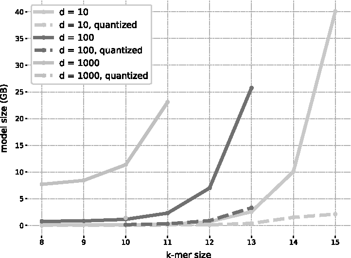end{document} . Their memory footprints are available in Figure 1.

OPEN IN VIEWER

FIG. 1.

Memory requirement of fastDNA models as a function of k-mer sizes. The embedding dimensions d shown are 10, 100, and 1000. The reported value is the size in GB of the model binary, the minimal size required both in RAM to train and load the model and on the disk to save it.

Contrary to VW, model size is completely determined by the user and does not depend on the number of possible classes T or on the vocabulary of the training database, which can become an advantage when T is large.

3.3.3. Performance

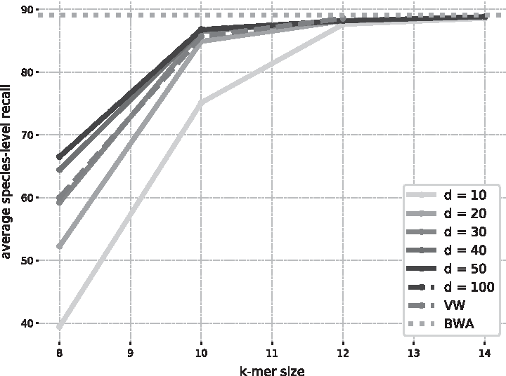
One first result from Figure 2 is that increasing the embedding dimension d above 50 brings no added benefit in classification quality, at the cost of larger prediction times and memory footprint. This could in theory be expected from Equation (4). Once d is greater than the number of classes, the matrix \documentclass{aastex}\usepackage{amsbsy}\usepackage{amsfonts}\usepackage{amssymb}\usepackage{bm}\usepackage{mathrsfs}\usepackage{pifont}\usepackage{stmaryrd}\usepackage{textcomp}\usepackage{portland, xspace}\usepackage{amsmath, amsxtra}\usepackage{upgreek}\pagestyle{empty}\DeclareMathSizes{10}{9}{7}{6}\begin{document} $$W{M^ \top }$$ \end{document} has maximal rank T, so the model is virtually the same as the standard “Bag of Words” model VW. The differences observed between the two are likely due to different optimization procedures and implementations.

OPEN IN VIEWER

FIG. 2.

Comparison between fastDNA and reference methods on the small data set. This figure shows the average species-level recall obtained by fastDNA trained for 50 epochs and a learning rate 0.1, for different values of k and d. The results are compared with VW and an alignment-based approach BWA-MEM. BWA, Burrows-Wheeler aligner; VW, Vowpal Wabbit.

Excessively lowering the dimension d under T harms the performance, especially for shorter k-mers. However, the gap between models \documentclass{aastex}\usepackage{amsbsy}\usepackage{amsfonts}\usepackage{amssymb}\usepackage{bm}\usepackage{mathrsfs}\usepackage{pifont}\usepackage{stmaryrd}\usepackage{textcomp}\usepackage{portland, xspace}\usepackage{amsmath, amsxtra}\usepackage{upgreek}\pagestyle{empty}\DeclareMathSizes{10}{9}{7}{6}\begin{document} $$d = 10$$ \end{document} and models \documentclass{aastex}\usepackage{amsbsy}\usepackage{amsfonts}\usepackage{amssymb}\usepackage{bm}\usepackage{mathrsfs}\usepackage{pifont}\usepackage{stmaryrd}\usepackage{textcomp}\usepackage{portland, xspace}\usepackage{amsmath, amsxtra}\usepackage{upgreek}\pagestyle{empty}\DeclareMathSizes{10}{9}{7}{6}\begin{document} $$d = 50$$ \end{document} vanishes as k increases, suggesting that—provided a sufficient vocabulary size—projecting k-mers to a lower dimensional space comes at little cost. Furthermore, models with longer k-mers but smaller dimension can achieve the same performance as a model with shorter k and greater dimension. The model \documentclass{aastex}\usepackage{amsbsy}\usepackage{amsfonts}\usepackage{amssymb}\usepackage{bm}\usepackage{mathrsfs}\usepackage{pifont}\usepackage{stmaryrd}\usepackage{textcomp}\usepackage{portland, xspace}\usepackage{amsmath, amsxtra}\usepackage{upgreek}\pagestyle{empty}\DeclareMathSizes{10}{9}{7}{6}\begin{document} $$k = 14 , d = 10$$ \end{document} has the same performance as \documentclass{aastex}\usepackage{amsbsy}\usepackage{amsfonts}\usepackage{amssymb}\usepackage{bm}\usepackage{mathrsfs}\usepackage{pifont}\usepackage{stmaryrd}\usepackage{textcomp}\usepackage{portland, xspace}\usepackage{amsmath, amsxtra}\usepackage{upgreek}\pagestyle{empty}\DeclareMathSizes{10}{9}{7}{6}\begin{document} $$k = 12 , d = 50$$ \end{document} .

Finally, classification performance for values of k greater than 12 is competitive with alignment-based method BWA, which confirms that machine learning approaches can be relevant for this problem of taxonomic binning.

3.4. Large data set

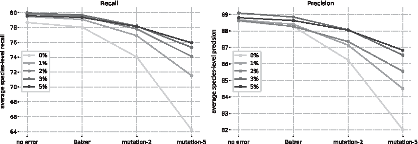
We report the classification performance, measured by average species-level recall and precision of fastDNA on the validation sets described in Section 3.1. The influence of the training noise is shown in Figure 3.

OPEN IN VIEWER

FIG. 3.

Performance on the large data set of fastDNA trained with different mutation rates. k-mer size and embedding dimension d are 13 and 100, respectively. The classification quality is measured on test sets generated with different sequencing error models.

As could be expected, greater levels of sequencing noise in the validation sets lead to degraded performances. Adding random mutations to the training reads curbs this effect. The greater the mutation rate is, the more robust the model becomes to higher levels of sequencing noise. Somewhat more surprisingly, a certain range of mutation rates also increases the performance on the validation reads with no sequencing noise. The regularization induced by these artificial errors is therefore beneficial for both sequencing noise and intraspecies heterogeneity. We found that the best rates of mutation were between 2% and 5%. The models trained with these levels of noise are better all-around than their no-noise counterparts.

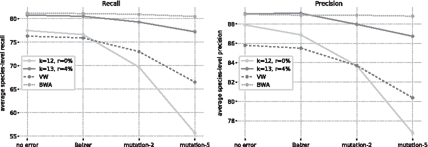
We compare the performance of fastDNA against that of VW and BWA in Figure 4. For small levels of sequencing errors, fastDNA is competitive with BWA. Greater levels in sequencing noise widen the gap between the two, as BWA is very robust to sequencing noise, dropping <1% for mutation-5.

OPEN IN VIEWER

FIG. 4.

Comparison between fastDNA and reference methods on the large data set. This figure shows the average species-level recall and precision obtained by fastDNA, VW, and BWA on the different validation sets. We show both the best configuration for fastDNA (k = 13, d = 100, r = 4%) and a similar one to VW (k = 12, d = 100, r = 0%) for a fair comparison.

3.5. Classification speed

Speed is of critical importance in taxonomic binning and is the main motivation behind exploring machine learning techniques. Classifying a read with fastDNA can be separated in two parts. It first reads the sequence, computes the indices of the k-mers contained in the read. and computes the read embedding by summing the k-mer embeddings. This step is of complexity \documentclass{aastex}\usepackage{amsbsy}\usepackage{amsfonts}\usepackage{amssymb}\usepackage{bm}\usepackage{mathrsfs}\usepackage{pifont}\usepackage{stmaryrd}\usepackage{textcomp}\usepackage{portland, xspace}\usepackage{amsmath, amsxtra}\usepackage{upgreek}\pagestyle{empty}\DeclareMathSizes{10}{9}{7}{6}\begin{document} $${ \cal O} ( dL )$$ \end{document} , where L is the read length (constant in our experiments). Second, class probabilities are computed by applying the linear classifier, this step is of complexity \documentclass{aastex}\usepackage{amsbsy}\usepackage{amsfonts}\usepackage{amssymb}\usepackage{bm}\usepackage{mathrsfs}\usepackage{pifont}\usepackage{stmaryrd}\usepackage{textcomp}\usepackage{portland, xspace}\usepackage{amsmath, amsxtra}\usepackage{upgreek}\pagestyle{empty}\DeclareMathSizes{10}{9}{7}{6}\begin{document} $${ \cal O} ( dT )$$ \end{document} . fastText and fastDNA offer a different loss function, the hierarchical softmax, that reduces this step to \documentclass{aastex}\usepackage{amsbsy}\usepackage{amsfonts}\usepackage{amssymb}\usepackage{bm}\usepackage{mathrsfs}\usepackage{pifont}\usepackage{stmaryrd}\usepackage{textcomp}\usepackage{portland, xspace}\usepackage{amsmath, amsxtra}\usepackage{upgreek}\pagestyle{empty}\DeclareMathSizes{10}{9}{7}{6}\begin{document} $${ \cal O} ( d \log ( T ) )$$ \end{document} , which can become useful in the case of very large T. To this per-read time-complexity must be added a fixed overhead, the time necessary for the model to be loaded from disk, of complexity \documentclass{aastex}\usepackage{amsbsy}\usepackage{amsfonts}\usepackage{amssymb}\usepackage{bm}\usepackage{mathrsfs}\usepackage{pifont}\usepackage{stmaryrd}\usepackage{textcomp}\usepackage{portland, xspace}\usepackage{amsmath, amsxtra}\usepackage{upgreek}\pagestyle{empty}\DeclareMathSizes{10}{9}{7}{6}\begin{document} $${ \cal O} ( dN + T )$$ \end{document} , where \documentclass{aastex}\usepackage{amsbsy}\usepackage{amsfonts}\usepackage{amssymb}\usepackage{bm}\usepackage{mathrsfs}\usepackage{pifont}\usepackage{stmaryrd}\usepackage{textcomp}\usepackage{portland, xspace}\usepackage{amsmath, amsxtra}\usepackage{upgreek}\pagestyle{empty}\DeclareMathSizes{10}{9}{7}{6}\begin{document} $$N{ = 4^k}$$ \end{document} is the vocabulary size. Due to the large values of \documentclass{aastex}\usepackage{amsbsy}\usepackage{amsfonts}\usepackage{amssymb}\usepackage{bm}\usepackage{mathrsfs}\usepackage{pifont}\usepackage{stmaryrd}\usepackage{textcomp}\usepackage{portland, xspace}\usepackage{amsmath, amsxtra}\usepackage{upgreek}\pagestyle{empty}\DeclareMathSizes{10}{9}{7}{6}\begin{document} $${4^k}$$ \end{document} , this can make up a significant portion of the total time. Moreover, we observe in practice a longer memory access time for larger vectors. These are the two reasons for the time gap observed between classifications with models of same embedding dimension d but different k.

The total time complexity for predicting a data set with n samples is therefore \documentclass{aastex}\usepackage{amsbsy}\usepackage{amsfonts}\usepackage{amssymb}\usepackage{bm}\usepackage{mathrsfs}\usepackage{pifont}\usepackage{stmaryrd}\usepackage{textcomp}\usepackage{portland, xspace}\usepackage{amsmath, amsxtra}\usepackage{upgreek}\pagestyle{empty}\DeclareMathSizes{10}{9}{7}{6}\begin{document} $${ \cal O} ( n ( dL + dT ) + dN )$$ \end{document} .

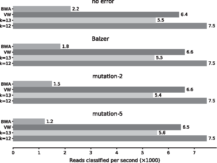
With reads of constant length, fastDNA and VW classify reads indiscriminately of their content and therefore yield equal classification times across the validation sets. However, BWAs speed degrades with the sequencing noise, which is easily explained. BWA searches iteratively on the number of mismatches z and stops once it gets a hit. It will therefore be slower if there are more mismatches between the testing and reference data.

We show in Figure 5 the classification speeds measured for the large data set. The values reported are for a single CPU (Intel Xeon E5-2450 v2 −2.5 GHz). We show fastDNA for \documentclass{aastex}\usepackage{amsbsy}\usepackage{amsfonts}\usepackage{amssymb}\usepackage{bm}\usepackage{mathrsfs}\usepackage{pifont}\usepackage{stmaryrd}\usepackage{textcomp}\usepackage{portland, xspace}\usepackage{amsmath, amsxtra}\usepackage{upgreek}\pagestyle{empty}\DeclareMathSizes{10}{9}{7}{6}\begin{document} $$d = 100$$ \end{document} and \documentclass{aastex}\usepackage{amsbsy}\usepackage{amsfonts}\usepackage{amssymb}\usepackage{bm}\usepackage{mathrsfs}\usepackage{pifont}\usepackage{stmaryrd}\usepackage{textcomp}\usepackage{portland, xspace}\usepackage{amsmath, amsxtra}\usepackage{upgreek}\pagestyle{empty}\DeclareMathSizes{10}{9}{7}{6}\begin{document} $$k = 12 , { \kern 1pt} \;13$$ \end{document} and VW. fastDNA and VW have similar classification times of ∼6, 7 · 10³ reads per minute. As remarked in Vervier et al. (2016), compositional approaches offer systematically better prediction times than BWA, with improvements of \documentclass{aastex}\usepackage{amsbsy}\usepackage{amsfonts}\usepackage{amssymb}\usepackage{bm}\usepackage{mathrsfs}\usepackage{pifont}\usepackage{stmaryrd}\usepackage{textcomp}\usepackage{portland, xspace}\usepackage{amsmath, amsxtra}\usepackage{upgreek}\pagestyle{empty}\DeclareMathSizes{10}{9}{7}{6}\begin{document} $$2 - 9 \times$$ \end{document} . This speed improvement increases with the mismatch between predicted sequences and reference genomes, therefore with both sequencing noise and intraspecies variations.

OPEN IN VIEWER

FIG. 5.

Comparison between fastDNA and reference methods on the large data set. This figure shows the average classification speed of the methods on the different test sets. Two versions of fastDNA are shown, one with k-mer size 12 and the other with k-mer size 13. Both have embedding dimension d = 100. The four test sets used were simulated with different sequencing error models.

References

1.
AnglyF.E., WillnerD., RohwerF., et al.2012. Grinder: a versatile amplicon and shotgun sequence simulator. Nucleic Acids Res. 40, e94.
2.
BalzerS., MaldeK., LanzénA., et al.2010. Characteristics of 454 pyrosequencing data—enabling realistic simulation with flowsim. Bioinformatics. 26, i420–i425.
3.
BojanowskiP., GraveE., JoulinA., et al.2017. Enriching word vectors with subword information. Trans. Assoc. Comput. Linguist. 5, 135–146.
4.
GroupN.H.W., PetersonJ., GargesS., et al.2009. The NIH human microbiome project. Genome Res. 19, 2317–2323.
5.
HusonD.H., AuchA. F., QiJ., et al.2007. MEGAN analysis of metagenomic data. Genome Res. 17, 377–386.
6.
JegouH., DouzeM., and SchmidC.2011. Product quantization for nearest neighbor search. IEEE Trans. Pattern. Anal. Mach. Intell. 33, 117–128.
7.
JoulinA., GraveE., BojanowskiP., et al.2016. Fasttext.zip: compressing text classification models. arXiv preprint arXiv: 1612.03651.
8.
JoulinA., GraveE., BojanowskiP., et al.2017. Bag of tricks for efficient text classification. Proceedings of the 15th Conference of the European Chapter of the Association for Computational Linguistics: Volume 2, Short Papers, pp. 427–431. Association for Computational Linguistics. Valencia, Spain.
9.
KorbelJ., AbyzovA., MuX., et al.2009. PEMer: a computational framework with simulation-based error models for inferring genomic structural variants from massive paired-end sequencing data. Genome Biol. 10, R23.
10.
LangmeadB., TrapnellC., PopM., et al.2009. Ultrafast and memory-efficient alignment of short DNA sequences to the human genome. Genome Biol. 10, R25.
11.
LeslieC., EskinE., and NobleW.2002. The spectrum kernel: a string kernel for SVM protein classification, 564–575. In AltmanR.B., DunkerA.K., HunterL., LauerdaleK., and KleinT.E., eds. Proceedings of the Pacific Symposium on Biocomputing 2002. Singapore: World Scientific.
12.
LeslieC., EskinE., WestonJ., et al.2003. Mismatch string kernels for SVM protein classification. In BeckerS., ThrunS., and ObermayerK., eds. Advances in Neural Information Processing Systems 15. MIT Press, Cambridge, MA, USA. Pgs. 1441–1448.
13.
LiH.2013. Aligning sequence reads, clone sequences and assembly contigs with BWA-MEM. Tech. Rep. 1303.3997, arXiv.
14.
LiH., and DurbinR.2009. Fast and accurate short read alignment with Burrows-Wheeler transform. Bioinformatics. 25, 1754–1760.
15.
LuoY., YuY.W., ZengJ., et al.2017. Metagenomic binning through low density hashing. Bioinformatics. 35, 219–226 (Jan.15, 2019).
16.
MandeS.S., MohammedM.H., and GhoshT.S.2012. Classification of metagenomic sequences: methods and challenges. Briefings Bioinf. 13, 669–681.
17.
McHardyA.C., MartínH.G., TsirigosA., et al.2007. Accurate phylogenetic classification of variable-length DNA fragments. Nat. Methods. 4, 63–72.
18.
MikolovT., ChenK., CorradoG., et al.2013. Efficient estimation of word representations in vector space. Tech. Rep. 1301.3781, arXiv.
19.
ParksD.H., MacDonaldN.J., and BeikoR.G.2011. Classifying short genomic fragments from novel lineages using composition and homology. BMC Bioinf. 12, 328.
20.
PatilK.R., RouneL., and McHardyA.C.2012. The PhyloPythiaS web server for taxonomic assignment of metagenome sequences. PLoS One. 7, e38581.
21.
RiesenfeldC.S., SchlossP.D., and HandelsmanJ.2004. Metagenomics: genomic analysis of microbial communities. Annu. Rev. Genet. 38, 525–552.
22.
VervierK., MahéP., TournoudM., et al.2016. Large-scale machine learning for metagenomics sequence classification. Bioinformatics. 32, 1023–1032.
23.
WangQ., GarrityG.M., TiedjeJ.M., et al.2007. Naive bayesian classifier for rapid assignment of rRNA sequences into the new bacterial taxonomy. Appl. Environ. Microbiol. 73, 5261–5267.
24.
WoodD.E., and SalzbergS.L.2014. Kraken: ultrafast metagenomic sequence classification using exact alignments. Genome Biol. 15, R46.