Topographic factor models separate overlapping signals into latent spatial functions to identify correlation structure across observations. These methods require the underlying structure to be held fixed and are not robust to deviations commonly found across images. We present autoencoding topographic factors, a novel variational inference scheme, to decompose irregular observations on a lattice into a superposition of low-rank sources. By exploiting recent developments in variational autoencoders, we replace fixed sources with a nonlinear mapping that parameterizes an unnormalized distribution on the lattice. In doing so, we permit sources to drift dynamically, filtering residual differences in location across comparable areas of interest. This gives an implicit mapping to a unique latent representation while simultaneously forcing the posterior to model group variability in spatial structure. Simulation results and applications to functional imaging demonstrate the effectiveness of our method and its ability to outperform existing spatial factor models.
1. Introduction
The analysis of biomedical images has accelerated in recent years due to domain-specific methodologies developed for multiple application areas. Calcium imaging in neurons (Pnevmatikakis et al., 2016), transcriptome profiling from single cells (Svensson et al., 2017), and functional imaging of various biomarkers (Gershman et al., 2014; Manning et al., 2014a) are exciting examples. Latent variable models are the predominant method for visualizing and extracting structure in spatial data. These data are characterized by a location vector \documentclass{aastex}\usepackage{amsbsy}\usepackage{amsfonts}\usepackage{amssymb}\usepackage{bm}\usepackage{mathrsfs}\usepackage{pifont}\usepackage{stmaryrd}\usepackage{textcomp}\usepackage{portland, xspace}\usepackage{amsmath, amsxtra}\usepackage{upgreek}\pagestyle{empty}\DeclareMathSizes{10}{9}{7}{6}\begin{document}
$${{ \bf{x}}_i} \in { \rm{ \Omega }} \subseteq { \mathbb{R}^d}$$
\end{document} parameterizing each observation \documentclass{aastex}\usepackage{amsbsy}\usepackage{amsfonts}\usepackage{amssymb}\usepackage{bm}\usepackage{mathrsfs}\usepackage{pifont}\usepackage{stmaryrd}\usepackage{textcomp}\usepackage{portland, xspace}\usepackage{amsmath, amsxtra}\usepackage{upgreek}\pagestyle{empty}\DeclareMathSizes{10}{9}{7}{6}\begin{document}
$${ \bf{y}} \left( {{{ \bf{x}}_i}} \right)$$
\end{document}. Given a tensor \documentclass{aastex}\usepackage{amsbsy}\usepackage{amsfonts}\usepackage{amssymb}\usepackage{bm}\usepackage{mathrsfs}\usepackage{pifont}\usepackage{stmaryrd}\usepackage{textcomp}\usepackage{portland, xspace}\usepackage{amsmath, amsxtra}\usepackage{upgreek}\pagestyle{empty}\DeclareMathSizes{10}{9}{7}{6}\begin{document}
$${ \cal Y} \equiv \{ { \bf{y}} \left( {{{ \bf{x}}_1}} \right) , \cdots , { \bf{y}} \left( {{{ \bf{x}}_m}} \right) \} _{n = 1}^N$$
\end{document} of N realizations, each sequence of m correlated random variables \documentclass{aastex}\usepackage{amsbsy}\usepackage{amsfonts}\usepackage{amssymb}\usepackage{bm}\usepackage{mathrsfs}\usepackage{pifont}\usepackage{stmaryrd}\usepackage{textcomp}\usepackage{portland, xspace}\usepackage{amsmath, amsxtra}\usepackage{upgreek}\pagestyle{empty}\DeclareMathSizes{10}{9}{7}{6}\begin{document}
$$Y \left( {{{ \bf{x}}_1}} \right) , \cdots , Y \left( {{{ \bf{x}}_m}} \right)$$
\end{document}, a fundamental challenge is to identify a subset of physical locations that define areas of interest. To this end, lattice-based models formalize an encoding of a latent probability distribution over \documentclass{aastex}\usepackage{amsbsy}\usepackage{amsfonts}\usepackage{amssymb}\usepackage{bm}\usepackage{mathrsfs}\usepackage{pifont}\usepackage{stmaryrd}\usepackage{textcomp}\usepackage{portland, xspace}\usepackage{amsmath, amsxtra}\usepackage{upgreek}\pagestyle{empty}\DeclareMathSizes{10}{9}{7}{6}\begin{document}
$$Y \left( {{{ \bf{x}}_1}} \right) , \cdots , Y \left( {{{ \bf{x}}_m}} \right)$$
\end{document} to quantify statistical dependencies based on distance. This representation is often used for Gaussian process regression or Kriging methods to predict covariance structure between hidden variables and observed features across a physical location in an ensemble (Svensson et al., 2017). For example, extracting relevant voxels from a collection of functional images to discover a latent hemodynamic response enables comparing baseline versus pathological populations (Worsley et al., 1996).
Techniques such as robust principal component analysis (Candès et al., 2011), independent component analysis, and dictionary learning (DL) are commonly applied to blind source separation problems; however, they require an inherently linear demixing or deconvolution and may fail if there is no linear mixture that leads to independent outputs (Mukamel et al., 2009). Notably, these methods do not learn a distribution on the lattice that can be used to quantify uncertainty or to generate new data. Topographic factor models (Gershman et al., 2011, 2014; Manning et al., 2014a) are a family of Bayesian variational techniques for images that require underlying structure on the set of random variables to be held constant to produce a matrix factorization with spatially interpretable sources.
In this study, we develop autoencoding topographic factors (AETF), a novel Bayesian algorithm, to infer spatial dependencies by decomposing observations on a lattice into a weighted set of low-rank sources. We are particularly interested in a solution that generalizes to unseen data and that is robust to noncollocated regions of interest. The key insight of AETF is to leverage recent advances in variational inference (Gershman et al., 2014; Ranganath et al., 2014) and stochastic gradient variational Bayes (Kingma and Welling, 2013; Rezende et al., 2014) to learn a latent probability model that preserves group variability in spatial structure. Our contributions are to combine two paradigms where convolutional neural networks define the loading matrix, and the factor matrix itself maps data to source functions that transform across observations. This is achieved without hard coding hyperparameters that control an a-priori generative model. In doing so, we remove the propensity on initialization of domain-specific priors. Experiments on two simulated data sets and on functional imaging data show that our model returns a higher proportion of variance explained than existing topographic factor models.
This article is organized as follows: Section 2 reviews related methods for blind source separation. Section 3 defines the model we propose for spatial factor analysis. Section 4 provides experimental results. Section 5 concludes and discusses future work.
2. Related Work
Non-negative matrix factorization has been adapted to calcium imaging data to infer both location and spiking dynamics of neurons from fluorescence movies (Friedrich et al., 2015; Pnevmatikakis et al., 2016). To facilitate inference, significant domain-specific prepossessing must be done to constrain the region of interest to patches and model spatial background structure. A more general approach to factor analysis for space-time variation involves identifying a common set of shared factors whose time varying dynamics are modeled with autoregressive weights (Lopes et al., 2008). Our method differs in that we allow each observation to have a unique set of factors generated by a common nonlinear mapping from the input space. In the case of spatial dynamic factor analysis, Bayesian inference is performed with a reversible jump MCMC algorithm whose convergence is difficult to assess and must be tailored for the problem at hand.
Topographic factor analysis (TFA) for modeling functional magnetic resonance imaging via factor decomposition was proposed (Manning et al., 2014a) and fit using Black Box VI (Ranganath et al., 2014). Our approach uses similar spatial functions and a posterior, which is mean field in time, however (Manning et al., 2014a), hard codes the structure of the factors, which are shared across observations. These parameters are often prefit using a preprocessing algorithm. Previous models are unable to capture the variation among observations while fitting individual-specific factors. In this sense, we develop a robust and expressive posterior distribution that does not require hand tuning hyperparameters for the priors. In addition, the TFA model does not generalize to unseen data and suffers linear parameter growth with respect to the size of the data set.
3. Autoencoding Topographic Factors
3.1 Standard lattice modeling
Following the convention of factor analysis, we assume that our data \documentclass{aastex}\usepackage{amsbsy}\usepackage{amsfonts}\usepackage{amssymb}\usepackage{bm}\usepackage{mathrsfs}\usepackage{pifont}\usepackage{stmaryrd}\usepackage{textcomp}\usepackage{portland, xspace}\usepackage{amsmath, amsxtra}\usepackage{upgreek}\pagestyle{empty}\DeclareMathSizes{10}{9}{7}{6}\begin{document}
$${ \bf{Y}} \in { \mathbb{R}^{N \times V}}$$
\end{document} can be decomposed into a set of unobserved weights and latent factors. We use N to denote the number of observations (images), K the number of sources, and V the number of lattice positions (voxels). We are discussing lattices in both 2D and 3D for our analysis. Each latent source is defined using a function that assigns a value to each point on the lattice (in voxel space) based on its location. For example, using the multivariate normal (MVN):
\documentclass{aastex}\usepackage{amsbsy}\usepackage{amsfonts}\usepackage{amssymb}\usepackage{bm}\usepackage{mathrsfs}\usepackage{pifont}\usepackage{stmaryrd}\usepackage{textcomp}\usepackage{portland, xspace}\usepackage{amsmath, amsxtra}\usepackage{upgreek}\pagestyle{empty}\DeclareMathSizes{10}{9}{7}{6}\begin{document}
\begin{align*}
K ( { { \bf { x } } _i } \vert \mu , { \bf { \Sigma } } ) = exp \ { - \frac { 1 } { 2 } { ( { { \bf { x } } _i } - \mu ) ^T } { { \bf { \Sigma } } ^ { - 1 } } \left( { { { \bf { x } } _i } - \mu } \right) \ } . \tag { 1 }
\end{align*}
\end{document}
We posit each observation \documentclass{aastex}\usepackage{amsbsy}\usepackage{amsfonts}\usepackage{amssymb}\usepackage{bm}\usepackage{mathrsfs}\usepackage{pifont}\usepackage{stmaryrd}\usepackage{textcomp}\usepackage{portland, xspace}\usepackage{amsmath, amsxtra}\usepackage{upgreek}\pagestyle{empty}\DeclareMathSizes{10}{9}{7}{6}\begin{document}
$${{ \bf{y}}_n} \in { \mathbb{R}^{1 \times V}}$$
\end{document} has a low-rank approximation that is a product of factor loadings \documentclass{aastex}\usepackage{amsbsy}\usepackage{amsfonts}\usepackage{amssymb}\usepackage{bm}\usepackage{mathrsfs}\usepackage{pifont}\usepackage{stmaryrd}\usepackage{textcomp}\usepackage{portland, xspace}\usepackage{amsmath, amsxtra}\usepackage{upgreek}\pagestyle{empty}\DeclareMathSizes{10}{9}{7}{6}\begin{document}
$${{ \bf{w}}_n} \in { \mathbb{R}^{1 \times K}}$$
\end{document} and a factor matrix \documentclass{aastex}\usepackage{amsbsy}\usepackage{amsfonts}\usepackage{amssymb}\usepackage{bm}\usepackage{mathrsfs}\usepackage{pifont}\usepackage{stmaryrd}\usepackage{textcomp}\usepackage{portland, xspace}\usepackage{amsmath, amsxtra}\usepackage{upgreek}\pagestyle{empty}\DeclareMathSizes{10}{9}{7}{6}\begin{document}
$${ \bf{F}} \in { \mathbb{R}^{K \times V}}$$
\end{document}. The generative distribution of our model factorizes using a Gaussian as follows:
\documentclass{aastex}\usepackage{amsbsy}\usepackage{amsfonts}\usepackage{amssymb}\usepackage{bm}\usepackage{mathrsfs}\usepackage{pifont}\usepackage{stmaryrd}\usepackage{textcomp}\usepackage{portland, xspace}\usepackage{amsmath, amsxtra}\usepackage{upgreek}\pagestyle{empty}\DeclareMathSizes{10}{9}{7}{6}\begin{document}
\begin{align*}
P \left( { \bf{Y}} \right) = \mathop \prod \limits_{n = 1}^N { \rm{ }}P \left( {{{ \bf{y}}_n}} \right). \tag{2}
\end{align*}
\end{document}\documentclass{aastex}\usepackage{amsbsy}\usepackage{amsfonts}\usepackage{amssymb}\usepackage{bm}\usepackage{mathrsfs}\usepackage{pifont}\usepackage{stmaryrd}\usepackage{textcomp}\usepackage{portland, xspace}\usepackage{amsmath, amsxtra}\usepackage{upgreek}\pagestyle{empty}\DeclareMathSizes{10}{9}{7}{6}\begin{document}
\begin{align*}
P \left( {{{ \bf{y}}_n}} \right) = { \cal N} ( {{ \bf{y}}_n} \vert {{ \bf{w}}_n}{ \bf{F}} , \sigma _y^2 ) , \tag{3}
\end{align*}
\end{document}
where \documentclass{aastex}\usepackage{amsbsy}\usepackage{amsfonts}\usepackage{amssymb}\usepackage{bm}\usepackage{mathrsfs}\usepackage{pifont}\usepackage{stmaryrd}\usepackage{textcomp}\usepackage{portland, xspace}\usepackage{amsmath, amsxtra}\usepackage{upgreek}\pagestyle{empty}\DeclareMathSizes{10}{9}{7}{6}\begin{document}
$$\sigma _y^2$$
\end{document} denotes the location or voxel noise. In a study by Manning (Manning et al., 2014b), radial basis source functions \documentclass{aastex}\usepackage{amsbsy}\usepackage{amsfonts}\usepackage{amssymb}\usepackage{bm}\usepackage{mathrsfs}\usepackage{pifont}\usepackage{stmaryrd}\usepackage{textcomp}\usepackage{portland, xspace}\usepackage{amsmath, amsxtra}\usepackage{upgreek}\pagestyle{empty}\DeclareMathSizes{10}{9}{7}{6}\begin{document}
$${f_k} \in { \mathbb{R}^V}$$
\end{document} are used to generate basis images and to define F, the source image matrix. In general, rows of F are computed by evaluating each of the K source functions at all V lattice points of the voxel space.
While it is common to focus on \documentclass{aastex}\usepackage{amsbsy}\usepackage{amsfonts}\usepackage{amssymb}\usepackage{bm}\usepackage{mathrsfs}\usepackage{pifont}\usepackage{stmaryrd}\usepackage{textcomp}\usepackage{portland, xspace}\usepackage{amsmath, amsxtra}\usepackage{upgreek}\pagestyle{empty}\DeclareMathSizes{10}{9}{7}{6}\begin{document}
$${ \bf{ \Sigma }} = \sigma { \bf{I}}$$
\end{document} or the MVN case in which \documentclass{aastex}\usepackage{amsbsy}\usepackage{amsfonts}\usepackage{amssymb}\usepackage{bm}\usepackage{mathrsfs}\usepackage{pifont}\usepackage{stmaryrd}\usepackage{textcomp}\usepackage{portland, xspace}\usepackage{amsmath, amsxtra}\usepackage{upgreek}\pagestyle{empty}\DeclareMathSizes{10}{9}{7}{6}\begin{document}
$${ \bf{ \Sigma }}$$
\end{document} is full, a larger class of kernels are supported through the Matérn family of covariance functions. In this study, \documentclass{aastex}\usepackage{amsbsy}\usepackage{amsfonts}\usepackage{amssymb}\usepackage{bm}\usepackage{mathrsfs}\usepackage{pifont}\usepackage{stmaryrd}\usepackage{textcomp}\usepackage{portland, xspace}\usepackage{amsmath, amsxtra}\usepackage{upgreek}\pagestyle{empty}\DeclareMathSizes{10}{9}{7}{6}\begin{document}
$${K_ \nu } \left( \cdot \right)$$
\end{document} is the modified Bessel function of the second kind with order parameter \documentclass{aastex}\usepackage{amsbsy}\usepackage{amsfonts}\usepackage{amssymb}\usepackage{bm}\usepackage{mathrsfs}\usepackage{pifont}\usepackage{stmaryrd}\usepackage{textcomp}\usepackage{portland, xspace}\usepackage{amsmath, amsxtra}\usepackage{upgreek}\pagestyle{empty}\DeclareMathSizes{10}{9}{7}{6}\begin{document}
$$\nu$$
\end{document}, where \documentclass{aastex}\usepackage{amsbsy}\usepackage{amsfonts}\usepackage{amssymb}\usepackage{bm}\usepackage{mathrsfs}\usepackage{pifont}\usepackage{stmaryrd}\usepackage{textcomp}\usepackage{portland, xspace}\usepackage{amsmath, amsxtra}\usepackage{upgreek}\pagestyle{empty}\DeclareMathSizes{10}{9}{7}{6}\begin{document}
$$\rho$$
\end{document} defines correlation length and \documentclass{aastex}\usepackage{amsbsy}\usepackage{amsfonts}\usepackage{amssymb}\usepackage{bm}\usepackage{mathrsfs}\usepackage{pifont}\usepackage{stmaryrd}\usepackage{textcomp}\usepackage{portland, xspace}\usepackage{amsmath, amsxtra}\usepackage{upgreek}\pagestyle{empty}\DeclareMathSizes{10}{9}{7}{6}\begin{document}
$$\left\lfloor \nu \right\rfloor$$
\end{document} describes the smoothness of the process. \documentclass{aastex}\usepackage{amsbsy}\usepackage{amsfonts}\usepackage{amssymb}\usepackage{bm}\usepackage{mathrsfs}\usepackage{pifont}\usepackage{stmaryrd}\usepackage{textcomp}\usepackage{portland, xspace}\usepackage{amsmath, amsxtra}\usepackage{upgreek}\pagestyle{empty}\DeclareMathSizes{10}{9}{7}{6}\begin{document}
$${ \rm{ \Gamma }} \left( \cdot \right)$$
\end{document} is the gamma function.
\documentclass{aastex}\usepackage{amsbsy}\usepackage{amsfonts}\usepackage{amssymb}\usepackage{bm}\usepackage{mathrsfs}\usepackage{pifont}\usepackage{stmaryrd}\usepackage{textcomp}\usepackage{portland, xspace}\usepackage{amsmath, amsxtra}\usepackage{upgreek}\pagestyle{empty}\DeclareMathSizes{10}{9}{7}{6}\begin{document}
\begin{align*}
K ( { { \bf { x } } _i } \vert \mu , \nu ) = \frac { 1 } { { { \rm { \Gamma } } \left( \nu \right) { 2^ { \nu - 1 } } } } { ( \frac { { \sqrt { 2 \nu } } } { \rho } \cdot \vert \vert { { \bf { x } } _i } - \mu \vert \vert ) ^ \nu } { K_ \nu } \left( { \frac { { \sqrt { 2 \nu } } } { \rho } \vert \vert { { \bf { x } } _i } - \mu \vert \vert } \right).
\end{align*}
\end{document}
The above simplifies for half-integer values of \documentclass{aastex}\usepackage{amsbsy}\usepackage{amsfonts}\usepackage{amssymb}\usepackage{bm}\usepackage{mathrsfs}\usepackage{pifont}\usepackage{stmaryrd}\usepackage{textcomp}\usepackage{portland, xspace}\usepackage{amsmath, amsxtra}\usepackage{upgreek}\pagestyle{empty}\DeclareMathSizes{10}{9}{7}{6}\begin{document}
$$\nu$$
\end{document} and reduces to the rational quadratic function with \documentclass{aastex}\usepackage{amsbsy}\usepackage{amsfonts}\usepackage{amssymb}\usepackage{bm}\usepackage{mathrsfs}\usepackage{pifont}\usepackage{stmaryrd}\usepackage{textcomp}\usepackage{portland, xspace}\usepackage{amsmath, amsxtra}\usepackage{upgreek}\pagestyle{empty}\DeclareMathSizes{10}{9}{7}{6}\begin{document}
$$\nu , \rho > 0$$
\end{document} to express a scale mixture of squared exponentials:
\documentclass{aastex}\usepackage{amsbsy}\usepackage{amsfonts}\usepackage{amssymb}\usepackage{bm}\usepackage{mathrsfs}\usepackage{pifont}\usepackage{stmaryrd}\usepackage{textcomp}\usepackage{portland, xspace}\usepackage{amsmath, amsxtra}\usepackage{upgreek}\pagestyle{empty}\DeclareMathSizes{10}{9}{7}{6}\begin{document}
\begin{align*}
K ( { { \bf { x } } _i } \vert \mu , \nu , \rho ) = { \left( { 1 + { \frac { \vert \vert { { \bf { x } } _i } - \mu \vert { \vert ^2 } } { 2 \nu { \rho ^2 } } } } \right) ^ { - \nu } } . \tag { 4 }
\end{align*}
\end{document}
Samples from the Gaussian process are \documentclass{aastex}\usepackage{amsbsy}\usepackage{amsfonts}\usepackage{amssymb}\usepackage{bm}\usepackage{mathrsfs}\usepackage{pifont}\usepackage{stmaryrd}\usepackage{textcomp}\usepackage{portland, xspace}\usepackage{amsmath, amsxtra}\usepackage{upgreek}\pagestyle{empty}\DeclareMathSizes{10}{9}{7}{6}\begin{document}
$$\left\lfloor { \nu - 1} \right\rfloor$$
\end{document} times differentiable producing the radial basis function (RBF) case when \documentclass{aastex}\usepackage{amsbsy}\usepackage{amsfonts}\usepackage{amssymb}\usepackage{bm}\usepackage{mathrsfs}\usepackage{pifont}\usepackage{stmaryrd}\usepackage{textcomp}\usepackage{portland, xspace}\usepackage{amsmath, amsxtra}\usepackage{upgreek}\pagestyle{empty}\DeclareMathSizes{10}{9}{7}{6}\begin{document}
$$\nu \to \infty$$
\end{document}. As with the above, the choice of distance metric can produce isotropy or anisotropy.
We are interested in the posterior distribution, involving integrating over a set of possible values for the latent variables:
\documentclass{aastex}\usepackage{amsbsy}\usepackage{amsfonts}\usepackage{amssymb}\usepackage{bm}\usepackage{mathrsfs}\usepackage{pifont}\usepackage{stmaryrd}\usepackage{textcomp}\usepackage{portland, xspace}\usepackage{amsmath, amsxtra}\usepackage{upgreek}\pagestyle{empty}\DeclareMathSizes{10}{9}{7}{6}\begin{document}
\begin{align*}
P ( { \bf { W } } , { \bf { F } } \vert { \bf { Y } } ) = { \frac { P \left( { { \bf { Y } } , { \bf { W } } , { \bf { F } } } \right) } { P \left( { \bf { Y } } \right) } } . \tag { 5 }
\end{align*}
\end{document}\documentclass{aastex}\usepackage{amsbsy}\usepackage{amsfonts}\usepackage{amssymb}\usepackage{bm}\usepackage{mathrsfs}\usepackage{pifont}\usepackage{stmaryrd}\usepackage{textcomp}\usepackage{portland, xspace}\usepackage{amsmath, amsxtra}\usepackage{upgreek}\pagestyle{empty}\DeclareMathSizes{10}{9}{7}{6}\begin{document}
\begin{align*}
P \left( { \bf{Y}} \right) = \int \int \smallint { \rm{ }} \smallint { \rm{ }}P \left( {{ \bf{Y}} , { \bf{W}} , { \bf{F}}} \right) d{ \bf{W}}d{ \bf{F}}. \tag{6}
\end{align*}
\end{document}
The problem is in general intractable to compute. To perform variational inference, a mean field distribution is defined in which each variable is independent:
\documentclass{aastex}\usepackage{amsbsy}\usepackage{amsfonts}\usepackage{amssymb}\usepackage{bm}\usepackage{mathrsfs}\usepackage{pifont}\usepackage{stmaryrd}\usepackage{textcomp}\usepackage{portland, xspace}\usepackage{amsmath, amsxtra}\usepackage{upgreek}\pagestyle{empty}\DeclareMathSizes{10}{9}{7}{6}\begin{document}
\begin{align*}
Q ( { \bf{W}} , { \bf{M}} , { \bf{ \Lambda }} ) = \mathop \prod \limits_{n = 1}^N { \rm{ }} \mathop \prod \limits_{k = 1}^K { \rm{ }}{ \cal N} ( {w_{n , k}} \vert {{ \bf{m}}_{{w_{n , k}}}} , {{ \bf{ \Lambda }}_{{w_{n , k}}}} ) { \cal N} ( {c_{n , k}} \vert {{ \bf{m}}_{{c_{n , k}}}} , {{ \bf{ \Lambda }}_{{c_{n , k}}}} ) { \cal N} ( {s_{n , k}} \vert {{ \bf{m}}_{{s_{n , k}}}} , {{ \bf{ \Lambda }}_{{s_{n , k}}}} ). \tag{7}
\end{align*}
\end{document}
These allow drawing corresponding latent random variables for centers, width scales, and weights for the kth latent source:
\documentclass{aastex}\usepackage{amsbsy}\usepackage{amsfonts}\usepackage{amssymb}\usepackage{bm}\usepackage{mathrsfs}\usepackage{pifont}\usepackage{stmaryrd}\usepackage{textcomp}\usepackage{portland, xspace}\usepackage{amsmath, amsxtra}\usepackage{upgreek}\pagestyle{empty}\DeclareMathSizes{10}{9}{7}{6}\begin{document}
\begin{align*}
{Z_k} = \left\{ {{z_{c , k}} , {z_{s , k}} , {z_{w , k}}} \right\} , \tag{9}
\end{align*}
\end{document}
where \documentclass{aastex}\usepackage{amsbsy}\usepackage{amsfonts}\usepackage{amssymb}\usepackage{bm}\usepackage{mathrsfs}\usepackage{pifont}\usepackage{stmaryrd}\usepackage{textcomp}\usepackage{portland, xspace}\usepackage{amsmath, amsxtra}\usepackage{upgreek}\pagestyle{empty}\DeclareMathSizes{10}{9}{7}{6}\begin{document}
$${z_{ \xi , k}} \sim { \cal N} \left( {{{ \bf{m}}_{ \xi , k}} , { \bf{ \Lambda }}_{ \xi , k}^2} \right)$$
\end{document} for \documentclass{aastex}\usepackage{amsbsy}\usepackage{amsfonts}\usepackage{amssymb}\usepackage{bm}\usepackage{mathrsfs}\usepackage{pifont}\usepackage{stmaryrd}\usepackage{textcomp}\usepackage{portland, xspace}\usepackage{amsmath, amsxtra}\usepackage{upgreek}\pagestyle{empty}\DeclareMathSizes{10}{9}{7}{6}\begin{document}
$$\xi \in \left\{ {c , s , w} \right\} $$
\end{document}. Note that in the isotropic case \documentclass{aastex}\usepackage{amsbsy}\usepackage{amsfonts}\usepackage{amssymb}\usepackage{bm}\usepackage{mathrsfs}\usepackage{pifont}\usepackage{stmaryrd}\usepackage{textcomp}\usepackage{portland, xspace}\usepackage{amsmath, amsxtra}\usepackage{upgreek}\pagestyle{empty}\DeclareMathSizes{10}{9}{7}{6}\begin{document}
$$\phi \in { \mathbb{R}^{K \left( {D + 5} \right) }}$$
\end{document} and \documentclass{aastex}\usepackage{amsbsy}\usepackage{amsfonts}\usepackage{amssymb}\usepackage{bm}\usepackage{mathrsfs}\usepackage{pifont}\usepackage{stmaryrd}\usepackage{textcomp}\usepackage{portland, xspace}\usepackage{amsmath, amsxtra}\usepackage{upgreek}\pagestyle{empty}\DeclareMathSizes{10}{9}{7}{6}\begin{document}
$${ \bf{Z}} \in { \mathbb{R}^{K \left( {D + 2} \right) }}$$
\end{document} where D is the dimensionality of the lattice.
Across all \documentclass{aastex}\usepackage{amsbsy}\usepackage{amsfonts}\usepackage{amssymb}\usepackage{bm}\usepackage{mathrsfs}\usepackage{pifont}\usepackage{stmaryrd}\usepackage{textcomp}\usepackage{portland, xspace}\usepackage{amsmath, amsxtra}\usepackage{upgreek}\pagestyle{empty}\DeclareMathSizes{10}{9}{7}{6}\begin{document}
$$\xi , k$$
\end{document} one can define \documentclass{aastex}\usepackage{amsbsy}\usepackage{amsfonts}\usepackage{amssymb}\usepackage{bm}\usepackage{mathrsfs}\usepackage{pifont}\usepackage{stmaryrd}\usepackage{textcomp}\usepackage{portland, xspace}\usepackage{amsmath, amsxtra}\usepackage{upgreek}\pagestyle{empty}\DeclareMathSizes{10}{9}{7}{6}\begin{document}
$${{ \bf{m}}_ \phi } = { ( {{ \bf{m}}_{ \xi , k}} ) _{ \forall \xi , k}}$$
\end{document} and \documentclass{aastex}\usepackage{amsbsy}\usepackage{amsfonts}\usepackage{amssymb}\usepackage{bm}\usepackage{mathrsfs}\usepackage{pifont}\usepackage{stmaryrd}\usepackage{textcomp}\usepackage{portland, xspace}\usepackage{amsmath, amsxtra}\usepackage{upgreek}\pagestyle{empty}\DeclareMathSizes{10}{9}{7}{6}\begin{document}
$${{ \bf{ \Sigma }}_ \phi } = {{ \bf{ \Lambda }}_ \phi }{ \bf{ \Lambda }}_ \phi ^T$$
\end{document} for \documentclass{aastex}\usepackage{amsbsy}\usepackage{amsfonts}\usepackage{amssymb}\usepackage{bm}\usepackage{mathrsfs}\usepackage{pifont}\usepackage{stmaryrd}\usepackage{textcomp}\usepackage{portland, xspace}\usepackage{amsmath, amsxtra}\usepackage{upgreek}\pagestyle{empty}\DeclareMathSizes{10}{9}{7}{6}\begin{document}
$${{ \bf{ \Lambda }}_ \phi } = { ( {{ \bf{ \Lambda }}_{ \xi , k}} ) _{ \forall \xi , k}}$$
\end{document}, thus the parameters \documentclass{aastex}\usepackage{amsbsy}\usepackage{amsfonts}\usepackage{amssymb}\usepackage{bm}\usepackage{mathrsfs}\usepackage{pifont}\usepackage{stmaryrd}\usepackage{textcomp}\usepackage{portland, xspace}\usepackage{amsmath, amsxtra}\usepackage{upgreek}\pagestyle{empty}\DeclareMathSizes{10}{9}{7}{6}\begin{document}
$${{ \bf{m}}_ \phi } , {{ \bf{ \Sigma }}_ \phi }$$
\end{document} denote the means and covariances used to draw Z. Z then defines F, by fk being a Gaussian function with parameters \documentclass{aastex}\usepackage{amsbsy}\usepackage{amsfonts}\usepackage{amssymb}\usepackage{bm}\usepackage{mathrsfs}\usepackage{pifont}\usepackage{stmaryrd}\usepackage{textcomp}\usepackage{portland, xspace}\usepackage{amsmath, amsxtra}\usepackage{upgreek}\pagestyle{empty}\DeclareMathSizes{10}{9}{7}{6}\begin{document}
$${z_{c , k}}$$
\end{document} and \documentclass{aastex}\usepackage{amsbsy}\usepackage{amsfonts}\usepackage{amssymb}\usepackage{bm}\usepackage{mathrsfs}\usepackage{pifont}\usepackage{stmaryrd}\usepackage{textcomp}\usepackage{portland, xspace}\usepackage{amsmath, amsxtra}\usepackage{upgreek}\pagestyle{empty}\DeclareMathSizes{10}{9}{7}{6}\begin{document}
$${z_{s , k}}$$
\end{document}.
3.2. Autoencoding topographic factors
The idea of AETF is to replace the fixed latent sources by defining a function that parameterizes Z using the output of a probabilistic encoder. The encoder creates an implicit mapping from each \documentclass{aastex}\usepackage{amsbsy}\usepackage{amsfonts}\usepackage{amssymb}\usepackage{bm}\usepackage{mathrsfs}\usepackage{pifont}\usepackage{stmaryrd}\usepackage{textcomp}\usepackage{portland, xspace}\usepackage{amsmath, amsxtra}\usepackage{upgreek}\pagestyle{empty}\DeclareMathSizes{10}{9}{7}{6}\begin{document}
$${{ \bf{y}}_n} \in { \bf{Y}}$$
\end{document} across a set of observations to a unique factor representation, while requiring that ϕ encodes the group variability in spatial structure.
where \documentclass{aastex}\usepackage{amsbsy}\usepackage{amsfonts}\usepackage{amssymb}\usepackage{bm}\usepackage{mathrsfs}\usepackage{pifont}\usepackage{stmaryrd}\usepackage{textcomp}\usepackage{portland, xspace}\usepackage{amsmath, amsxtra}\usepackage{upgreek}\pagestyle{empty}\DeclareMathSizes{10}{9}{7}{6}\begin{document}
$${f_k} \left( {{{ \bf{y}}_n}} \right)$$
\end{document} is the lattice values of a Gaussian function parameterized by \documentclass{aastex}\usepackage{amsbsy}\usepackage{amsfonts}\usepackage{amssymb}\usepackage{bm}\usepackage{mathrsfs}\usepackage{pifont}\usepackage{stmaryrd}\usepackage{textcomp}\usepackage{portland, xspace}\usepackage{amsmath, amsxtra}\usepackage{upgreek}\pagestyle{empty}\DeclareMathSizes{10}{9}{7}{6}\begin{document}
$${z_{c , k}} \left( {{{ \bf{y}}_n}} \right)$$
\end{document} and \documentclass{aastex}\usepackage{amsbsy}\usepackage{amsfonts}\usepackage{amssymb}\usepackage{bm}\usepackage{mathrsfs}\usepackage{pifont}\usepackage{stmaryrd}\usepackage{textcomp}\usepackage{portland, xspace}\usepackage{amsmath, amsxtra}\usepackage{upgreek}\pagestyle{empty}\DeclareMathSizes{10}{9}{7}{6}\begin{document}
$${z_{s , k}} \left( {{{ \bf{y}}_n}} \right)$$
\end{document}. \documentclass{aastex}\usepackage{amsbsy}\usepackage{amsfonts}\usepackage{amssymb}\usepackage{bm}\usepackage{mathrsfs}\usepackage{pifont}\usepackage{stmaryrd}\usepackage{textcomp}\usepackage{portland, xspace}\usepackage{amsmath, amsxtra}\usepackage{upgreek}\pagestyle{empty}\DeclareMathSizes{10}{9}{7}{6}\begin{document}
$${z_{ \xi , k}} \left( {{{ \bf{y}}_n}} \right)$$
\end{document} itself is a latent variable drawn from a normal distribution \documentclass{aastex}\usepackage{amsbsy}\usepackage{amsfonts}\usepackage{amssymb}\usepackage{bm}\usepackage{mathrsfs}\usepackage{pifont}\usepackage{stmaryrd}\usepackage{textcomp}\usepackage{portland, xspace}\usepackage{amsmath, amsxtra}\usepackage{upgreek}\pagestyle{empty}\DeclareMathSizes{10}{9}{7}{6}\begin{document}
$${z_{ \xi , k}} \left( {{{ \bf{y}}_n}} \right) \sim { \cal N} \left( {{{ \bf{m}}_{k , \xi , \phi }} \left( {{{ \bf{y}}_n}} \right) , {{ \bf{ \Lambda }}_{k , \xi , \phi }} \left( {{{ \bf{y}}_n}} \right) } \right)$$
\end{document} whose parameters are the encoder output.
Using the well-known reparameterization trick (Kingma and Welling, 2013; Rezende et al., 2014), we sample from \documentclass{aastex}\usepackage{amsbsy}\usepackage{amsfonts}\usepackage{amssymb}\usepackage{bm}\usepackage{mathrsfs}\usepackage{pifont}\usepackage{stmaryrd}\usepackage{textcomp}\usepackage{portland, xspace}\usepackage{amsmath, amsxtra}\usepackage{upgreek}\pagestyle{empty}\DeclareMathSizes{10}{9}{7}{6}\begin{document}
$$\varepsilon \sim { \cal N} \left( {0 , { \bf{I}}} \right)$$
\end{document} to compute the following as the Monte Carlo estimates of gradients have high variance:
\documentclass{aastex}\usepackage{amsbsy}\usepackage{amsfonts}\usepackage{amssymb}\usepackage{bm}\usepackage{mathrsfs}\usepackage{pifont}\usepackage{stmaryrd}\usepackage{textcomp}\usepackage{portland, xspace}\usepackage{amsmath, amsxtra}\usepackage{upgreek}\pagestyle{empty}\DeclareMathSizes{10}{9}{7}{6}\begin{document}
\begin{align*}
{{ \bf{Z}}_c} = { \mu _c} + \varepsilon \odot { \sigma _c}. \tag{13}
\end{align*}
\end{document}\documentclass{aastex}\usepackage{amsbsy}\usepackage{amsfonts}\usepackage{amssymb}\usepackage{bm}\usepackage{mathrsfs}\usepackage{pifont}\usepackage{stmaryrd}\usepackage{textcomp}\usepackage{portland, xspace}\usepackage{amsmath, amsxtra}\usepackage{upgreek}\pagestyle{empty}\DeclareMathSizes{10}{9}{7}{6}\begin{document}
\begin{align*}
{{ \bf{Z}}_s} = { \mu _s} + \varepsilon \odot { \sigma _s}. \tag{14}
\end{align*}
\end{document}
One is now free to choose the weights \documentclass{aastex}\usepackage{amsbsy}\usepackage{amsfonts}\usepackage{amssymb}\usepackage{bm}\usepackage{mathrsfs}\usepackage{pifont}\usepackage{stmaryrd}\usepackage{textcomp}\usepackage{portland, xspace}\usepackage{amsmath, amsxtra}\usepackage{upgreek}\pagestyle{empty}\DeclareMathSizes{10}{9}{7}{6}\begin{document}
$${{ \bf{Z}}_w} \in \phi$$
\end{document} as variational parameters of the recognition model or parameters with the generative model: \documentclass{aastex}\usepackage{amsbsy}\usepackage{amsfonts}\usepackage{amssymb}\usepackage{bm}\usepackage{mathrsfs}\usepackage{pifont}\usepackage{stmaryrd}\usepackage{textcomp}\usepackage{portland, xspace}\usepackage{amsmath, amsxtra}\usepackage{upgreek}\pagestyle{empty}\DeclareMathSizes{10}{9}{7}{6}\begin{document}
$${{ \bf{Z}}_w} \in \phi$$
\end{document}. Including the weights in φ gives the following:
\documentclass{aastex}\usepackage{amsbsy}\usepackage{amsfonts}\usepackage{amssymb}\usepackage{bm}\usepackage{mathrsfs}\usepackage{pifont}\usepackage{stmaryrd}\usepackage{textcomp}\usepackage{portland, xspace}\usepackage{amsmath, amsxtra}\usepackage{upgreek}\pagestyle{empty}\DeclareMathSizes{10}{9}{7}{6}\begin{document}
\begin{align*}
{{ \bf{Z}}_w} = { \mu _w} + \varepsilon \odot { \sigma _w}. \tag{15}
\end{align*}
\end{document}
When \documentclass{aastex}\usepackage{amsbsy}\usepackage{amsfonts}\usepackage{amssymb}\usepackage{bm}\usepackage{mathrsfs}\usepackage{pifont}\usepackage{stmaryrd}\usepackage{textcomp}\usepackage{portland, xspace}\usepackage{amsmath, amsxtra}\usepackage{upgreek}\pagestyle{empty}\DeclareMathSizes{10}{9}{7}{6}\begin{document}
$${{ \bf{Z}}_w} \notin \phi$$
\end{document}, we learn the weights as point estimates using the update rule:
\documentclass{aastex}\usepackage{amsbsy}\usepackage{amsfonts}\usepackage{amssymb}\usepackage{bm}\usepackage{mathrsfs}\usepackage{pifont}\usepackage{stmaryrd}\usepackage{textcomp}\usepackage{portland, xspace}\usepackage{amsmath, amsxtra}\usepackage{upgreek}\pagestyle{empty}\DeclareMathSizes{10}{9}{7}{6}\begin{document}
\begin{align*}
{{ \bf{W}}^{i + 1}} \leftarrow {{ \bf{W}}^i} \odot { \bf{YF}}{ ( {{ \bf{y}}_n} ) ^T} \O {{ \bf{W}}^i}{ \bf{F}} \left( {{{ \bf{y}}_n}} \right) { \bf{F}}{ ( {{ \bf{y}}_n} ) ^T}. \tag{16}
\end{align*}
\end{document}
Note that the problem is hard due to the nonconvexity in the source image matrix. With the parameters ϕ of the recognition model in hand, we have the full model specification. In contrast to standard autoencoder formalization, where the generative model involves a decoder whose parameters need to be inferred, AETF specifies the generative model. We thus compute the approximation \documentclass{aastex}\usepackage{amsbsy}\usepackage{amsfonts}\usepackage{amssymb}\usepackage{bm}\usepackage{mathrsfs}\usepackage{pifont}\usepackage{stmaryrd}\usepackage{textcomp}\usepackage{portland, xspace}\usepackage{amsmath, amsxtra}\usepackage{upgreek}\pagestyle{empty}\DeclareMathSizes{10}{9}{7}{6}\begin{document}
$${ \bf{y}} = { \bf{W}}\left({{{\bf{y}}_n}}\right) \cdot { \bf{F}}
\left({{{\bf{y}}_n}}\right)$$
\end{document}.
Standard autoencoders learn the respective encoder/decoder parameters \documentclass{aastex}\usepackage{amsbsy}\usepackage{amsfonts}\usepackage{amssymb}\usepackage{bm}\usepackage{mathrsfs}\usepackage{pifont}\usepackage{stmaryrd}\usepackage{textcomp}\usepackage{portland, xspace}\usepackage{amsmath, amsxtra}\usepackage{upgreek}\pagestyle{empty}\DeclareMathSizes{10}{9}{7}{6}\begin{document}
$$\theta , \phi$$
\end{document} by maximizing the conditional log likelihood \documentclass{aastex}\usepackage{amsbsy}\usepackage{amsfonts}\usepackage{amssymb}\usepackage{bm}\usepackage{mathrsfs}\usepackage{pifont}\usepackage{stmaryrd}\usepackage{textcomp}\usepackage{portland, xspace}\usepackage{amsmath, amsxtra}\usepackage{upgreek}\pagestyle{empty}\DeclareMathSizes{10}{9}{7}{6}\begin{document}
$${ \mathbb{E}_{q ( { \bf{z}} \vert {{ \bf{y}}^i} ) }} [ log{ \rm{ \; \;}}{p_ \theta } ( {{ \bf{y}}^i} \vert { \bf{z}} ) ]$$
\end{document} by differentiating through \documentclass{aastex}\usepackage{amsbsy}\usepackage{amsfonts}\usepackage{amssymb}\usepackage{bm}\usepackage{mathrsfs}\usepackage{pifont}\usepackage{stmaryrd}\usepackage{textcomp}\usepackage{portland, xspace}\usepackage{amsmath, amsxtra}\usepackage{upgreek}\pagestyle{empty}\DeclareMathSizes{10}{9}{7}{6}\begin{document}
$$g \leftarrow { \nabla _{ \theta , \phi }}{ \mathcal{L}^M} \left( { \theta , \phi {{ \bf{Y}}^M} , \varepsilon } \right)$$
\end{document} (Kingma and Welling, 2013; Rezende et al., 2014). AETF only needs to learn the encoder parameters ϕ, which is achieved by analogous maximization of the conditional log likelihood \documentclass{aastex}\usepackage{amsbsy}\usepackage{amsfonts}\usepackage{amssymb}\usepackage{bm}\usepackage{mathrsfs}\usepackage{pifont}\usepackage{stmaryrd}\usepackage{textcomp}\usepackage{portland, xspace}\usepackage{amsmath, amsxtra}\usepackage{upgreek}\pagestyle{empty}\DeclareMathSizes{10}{9}{7}{6}\begin{document}
$${ \mathbb{E}_{q ( { \bf{z}} \vert {{ \bf{y}}^i} ) }} [ log{ \rm{ \; \;}}p ( {{ \bf{y}}^i} \vert { \bf{z}} ) ]$$
\end{document}, differentiating through \documentclass{aastex}\usepackage{amsbsy}\usepackage{amsfonts}\usepackage{amssymb}\usepackage{bm}\usepackage{mathrsfs}\usepackage{pifont}\usepackage{stmaryrd}\usepackage{textcomp}\usepackage{portland, xspace}\usepackage{amsmath, amsxtra}\usepackage{upgreek}\pagestyle{empty}\DeclareMathSizes{10}{9}{7}{6}\begin{document}
$$g \leftarrow { \nabla _ \phi }{ \mathcal{L}^M} \left( { \phi {{ \bf{Y}}^M} , \varepsilon } \right)$$
\end{document}.
3.3. Implementation
The encoder takes as input an observation and outputs the parameters of the distributions over latent variables. Two recognition models are implemented, one with isotropic and another with full covariance source functions. The isotropic decoder receives as input the sampled latent space vector \documentclass{aastex}\usepackage{amsbsy}\usepackage{amsfonts}\usepackage{amssymb}\usepackage{bm}\usepackage{mathrsfs}\usepackage{pifont}\usepackage{stmaryrd}\usepackage{textcomp}\usepackage{portland, xspace}\usepackage{amsmath, amsxtra}\usepackage{upgreek}\pagestyle{empty}\DeclareMathSizes{10}{9}{7}{6}\begin{document}
$${ \bf{Z}} \in { \mathbb{R}^{k \left( {d + 2} \right) }}$$
\end{document}, including \documentclass{aastex}\usepackage{amsbsy}\usepackage{amsfonts}\usepackage{amssymb}\usepackage{bm}\usepackage{mathrsfs}\usepackage{pifont}\usepackage{stmaryrd}\usepackage{textcomp}\usepackage{portland, xspace}\usepackage{amsmath, amsxtra}\usepackage{upgreek}\pagestyle{empty}\DeclareMathSizes{10}{9}{7}{6}\begin{document}
$${{ \bf{Z}}_c} , { \rm{ \; \;}}{{ \bf{Z}}_s} , \ { \rm{and }} \ {{ \bf{Z}}_w}$$
\end{document}. Note that in the second case of a full covariance matrix \documentclass{aastex}\usepackage{amsbsy}\usepackage{amsfonts}\usepackage{amssymb}\usepackage{bm}\usepackage{mathrsfs}\usepackage{pifont}\usepackage{stmaryrd}\usepackage{textcomp}\usepackage{portland, xspace}\usepackage{amsmath, amsxtra}\usepackage{upgreek}\pagestyle{empty}\DeclareMathSizes{10}{9}{7}{6}\begin{document}
$${{ \bf{Z}}_{{{ \bf{s}}_{ \bf{ \Sigma }}}}}_k = { \bf{ \Lambda }}{{ \bf{ \Lambda }}^T}$$
\end{document}, we learn parameters \documentclass{aastex}\usepackage{amsbsy}\usepackage{amsfonts}\usepackage{amssymb}\usepackage{bm}\usepackage{mathrsfs}\usepackage{pifont}\usepackage{stmaryrd}\usepackage{textcomp}\usepackage{portland, xspace}\usepackage{amsmath, amsxtra}\usepackage{upgreek}\pagestyle{empty}\DeclareMathSizes{10}{9}{7}{6}\begin{document}
$${{ \bf{Z}}_{{{ \bf{s}}_{ \bf{ \Sigma }}}}} \in { \mathbb{R}^{kd \left( {d + 1} \right) / 2}}$$
\end{document}. The spatial factorization constraints of our probability model are imposed within the decoder. Thus, unlike traditional variational autoencoders where both the encoder and decoder are neural networks, AETF uses a neural network only for the encoder. The decoder uses the sampled latent space to reconstitute the input according to our imposed factorization and therefore is not parameterized by a neural network.
The encoder network can comprise any number of convolutional layers followed by any number of fully connected layers before the output layer. The convolutional layer executes an \documentclass{aastex}\usepackage{amsbsy}\usepackage{amsfonts}\usepackage{amssymb}\usepackage{bm}\usepackage{mathrsfs}\usepackage{pifont}\usepackage{stmaryrd}\usepackage{textcomp}\usepackage{portland, xspace}\usepackage{amsmath, amsxtra}\usepackage{upgreek}\pagestyle{empty}\DeclareMathSizes{10}{9}{7}{6}\begin{document}
$${L^{ \left( 1 \right) }} \otimes \cdots \otimes {L^{ \left( D \right) }}$$
\end{document} convolution along the number of lattice dimensions D (where L is specified for each layer) with k (the number of sources) output channels, a bias addition, a tanh nonlinearity, and max pooling with a \documentclass{aastex}\usepackage{amsbsy}\usepackage{amsfonts}\usepackage{amssymb}\usepackage{bm}\usepackage{mathrsfs}\usepackage{pifont}\usepackage{stmaryrd}\usepackage{textcomp}\usepackage{portland, xspace}\usepackage{amsmath, amsxtra}\usepackage{upgreek}\pagestyle{empty}\DeclareMathSizes{10}{9}{7}{6}\begin{document}
$${3^{ \left( 1 \right) }} \otimes \cdots \otimes {3^{ \left( D \right) }}$$
\end{document} kernel and a stride of 1. Our fully connected layers begin operating on the flattened output of the last convolutional layer or the flattened image if a convolution layer is not used. Their output dimensions are specified ratiometrically according to their output-to-input dimensions. Like most autoencoders, our encoder seeks to compress information. Thus, we only consider output-to-input ratios for our fully connected layers that are all less than or equal to 1. These fully connected layers invoke an affine transformation followed by a tanh nonlinearity.
Our final output layer varies according to the latent space parameter class. Those parameters that are means (\documentclass{aastex}\usepackage{amsbsy}\usepackage{amsfonts}\usepackage{amssymb}\usepackage{bm}\usepackage{mathrsfs}\usepackage{pifont}\usepackage{stmaryrd}\usepackage{textcomp}\usepackage{portland, xspace}\usepackage{amsmath, amsxtra}\usepackage{upgreek}\pagestyle{empty}\DeclareMathSizes{10}{9}{7}{6}\begin{document}
$${ \mu _c} , { \mu _s}$$
\end{document}, and \documentclass{aastex}\usepackage{amsbsy}\usepackage{amsfonts}\usepackage{amssymb}\usepackage{bm}\usepackage{mathrsfs}\usepackage{pifont}\usepackage{stmaryrd}\usepackage{textcomp}\usepackage{portland, xspace}\usepackage{amsmath, amsxtra}\usepackage{upgreek}\pagestyle{empty}\DeclareMathSizes{10}{9}{7}{6}\begin{document}
$${ \mu _e}$$
\end{document}) have no restrictions on their values except the last one, which must be positive. We handle this exception in the decoder. Therefore, we are free to use a vanilla affine transform as the output layers for these parameters. Conversely, those parameters that are standard deviations (\documentclass{aastex}\usepackage{amsbsy}\usepackage{amsfonts}\usepackage{amssymb}\usepackage{bm}\usepackage{mathrsfs}\usepackage{pifont}\usepackage{stmaryrd}\usepackage{textcomp}\usepackage{portland, xspace}\usepackage{amsmath, amsxtra}\usepackage{upgreek}\pagestyle{empty}\DeclareMathSizes{10}{9}{7}{6}\begin{document}
$${ \sigma _c} , { \sigma _s}$$
\end{document}, and \documentclass{aastex}\usepackage{amsbsy}\usepackage{amsfonts}\usepackage{amssymb}\usepackage{bm}\usepackage{mathrsfs}\usepackage{pifont}\usepackage{stmaryrd}\usepackage{textcomp}\usepackage{portland, xspace}\usepackage{amsmath, amsxtra}\usepackage{upgreek}\pagestyle{empty}\DeclareMathSizes{10}{9}{7}{6}\begin{document}
$${ \sigma _w}$$
\end{document}) must be greater than or equal to zero. Thus, for those standard deviations that parameterize our latent space, we use an affine transformation followed by a custom nonlinearity we call PostReAct (Positive Real Activation in Equation (17)). This nonlinearity is a piece-wise combination of a shifted ReLU and a decaying exponential. In this manner, we benefit from ReLU's positive regimen that avoids vanishing gradients that are common with double-saturating activations while avoiding the potential of neuron death associated with ReLU's negative regimen.
\documentclass{aastex}\usepackage{amsbsy}\usepackage{amsfonts}\usepackage{amssymb}\usepackage{bm}\usepackage{mathrsfs}\usepackage{pifont}\usepackage{stmaryrd}\usepackage{textcomp}\usepackage{portland, xspace}\usepackage{amsmath, amsxtra}\usepackage{upgreek}\pagestyle{empty}\DeclareMathSizes{10}{9}{7}{6}\begin{document}
\begin{align*}
{ \rm{ \Psi }} \left( \lambda \right) = \left\{ { \begin{matrix} {{ \rm{exp}} \left( \lambda \right) } & { , \lambda < 0} \\ { \lambda + 1} & { , \lambda \ge 0} \\ \end{matrix} } \right.. \tag{17}
\end{align*}
\end{document}
Our decoder has two responsibilities. First, it constructs the spatial factors using the \documentclass{aastex}\usepackage{amsbsy}\usepackage{amsfonts}\usepackage{amssymb}\usepackage{bm}\usepackage{mathrsfs}\usepackage{pifont}\usepackage{stmaryrd}\usepackage{textcomp}\usepackage{portland, xspace}\usepackage{amsmath, amsxtra}\usepackage{upgreek}\pagestyle{empty}\DeclareMathSizes{10}{9}{7}{6}\begin{document}
$${{ \bf{Z}}_c} \, \ { \rm{and }} \ {{ \bf{Z}}_s}$$
\end{document} latent space. However, and as aforementioned, \documentclass{aastex}\usepackage{amsbsy}\usepackage{amsfonts}\usepackage{amssymb}\usepackage{bm}\usepackage{mathrsfs}\usepackage{pifont}\usepackage{stmaryrd}\usepackage{textcomp}\usepackage{portland, xspace}\usepackage{amsmath, amsxtra}\usepackage{upgreek}\pagestyle{empty}\DeclareMathSizes{10}{9}{7}{6}\begin{document}
$${{ \bf{Z}}_s}$$
\end{document} arrives at the encoder on the incorrect support. The RBF function assumes this number is positive. We convert \documentclass{aastex}\usepackage{amsbsy}\usepackage{amsfonts}\usepackage{amssymb}\usepackage{bm}\usepackage{mathrsfs}\usepackage{pifont}\usepackage{stmaryrd}\usepackage{textcomp}\usepackage{portland, xspace}\usepackage{amsmath, amsxtra}\usepackage{upgreek}\pagestyle{empty}\DeclareMathSizes{10}{9}{7}{6}\begin{document}
$${{ \bf{Z}}_s}$$
\end{document} to the correct support in two ways. First, we pass it through a PostReAct nonlinearity. Second, we square it in our isotropic implementation. Equation (18) captures this process that we use for each of our basis image calculations. In this study, \documentclass{aastex}\usepackage{amsbsy}\usepackage{amsfonts}\usepackage{amssymb}\usepackage{bm}\usepackage{mathrsfs}\usepackage{pifont}\usepackage{stmaryrd}\usepackage{textcomp}\usepackage{portland, xspace}\usepackage{amsmath, amsxtra}\usepackage{upgreek}\pagestyle{empty}\DeclareMathSizes{10}{9}{7}{6}\begin{document}
$${f_k} \left( v \right)$$
\end{document} represents the value of the \documentclass{aastex}\usepackage{amsbsy}\usepackage{amsfonts}\usepackage{amssymb}\usepackage{bm}\usepackage{mathrsfs}\usepackage{pifont}\usepackage{stmaryrd}\usepackage{textcomp}\usepackage{portland, xspace}\usepackage{amsmath, amsxtra}\usepackage{upgreek}\pagestyle{empty}\DeclareMathSizes{10}{9}{7}{6}\begin{document}
$$k{ \rm{th}}$$
\end{document} RBF source at voxel position v. Unlike traditional RBF functions, we add a 1 to the denominator to clamp the source's width in a continuously differentiable manner. Before this modification, sampled \documentclass{aastex}\usepackage{amsbsy}\usepackage{amsfonts}\usepackage{amssymb}\usepackage{bm}\usepackage{mathrsfs}\usepackage{pifont}\usepackage{stmaryrd}\usepackage{textcomp}\usepackage{portland, xspace}\usepackage{amsmath, amsxtra}\usepackage{upgreek}\pagestyle{empty}\DeclareMathSizes{10}{9}{7}{6}\begin{document}
$${{ \bf{Z}}_s}$$
\end{document}, resulting in small source widths, produced exploding gradients for our optimizer. Once the decoder constructs the k basis images, it recombines them into a single image via a weighted summation that uses \documentclass{aastex}\usepackage{amsbsy}\usepackage{amsfonts}\usepackage{amssymb}\usepackage{bm}\usepackage{mathrsfs}\usepackage{pifont}\usepackage{stmaryrd}\usepackage{textcomp}\usepackage{portland, xspace}\usepackage{amsmath, amsxtra}\usepackage{upgreek}\pagestyle{empty}\DeclareMathSizes{10}{9}{7}{6}\begin{document}
$${{ \bf{Z}}_w}$$
\end{document}.
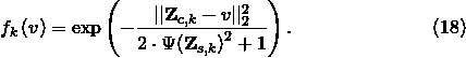
We present two encoder network architectures in Figure 1. Our first uses only a \documentclass{aastex}\usepackage{amsbsy}\usepackage{amsfonts}\usepackage{amssymb}\usepackage{bm}\usepackage{mathrsfs}\usepackage{pifont}\usepackage{stmaryrd}\usepackage{textcomp}\usepackage{portland, xspace}\usepackage{amsmath, amsxtra}\usepackage{upgreek}\pagestyle{empty}\DeclareMathSizes{10}{9}{7}{6}\begin{document}
$$7 \times 7$$
\end{document} convolutional layer followed by the output layer. Our second uses—in order of appearance—a \documentclass{aastex}\usepackage{amsbsy}\usepackage{amsfonts}\usepackage{amssymb}\usepackage{bm}\usepackage{mathrsfs}\usepackage{pifont}\usepackage{stmaryrd}\usepackage{textcomp}\usepackage{portland, xspace}\usepackage{amsmath, amsxtra}\usepackage{upgreek}\pagestyle{empty}\DeclareMathSizes{10}{9}{7}{6}\begin{document}
$$7 \times 7$$
\end{document} convolutional layer, a \documentclass{aastex}\usepackage{amsbsy}\usepackage{amsfonts}\usepackage{amssymb}\usepackage{bm}\usepackage{mathrsfs}\usepackage{pifont}\usepackage{stmaryrd}\usepackage{textcomp}\usepackage{portland, xspace}\usepackage{amsmath, amsxtra}\usepackage{upgreek}\pagestyle{empty}\DeclareMathSizes{10}{9}{7}{6}\begin{document}
$$5 \times 5$$
\end{document} convolutional layer, a \documentclass{aastex}\usepackage{amsbsy}\usepackage{amsfonts}\usepackage{amssymb}\usepackage{bm}\usepackage{mathrsfs}\usepackage{pifont}\usepackage{stmaryrd}\usepackage{textcomp}\usepackage{portland, xspace}\usepackage{amsmath, amsxtra}\usepackage{upgreek}\pagestyle{empty}\DeclareMathSizes{10}{9}{7}{6}\begin{document}
$$1:1$$
\end{document} output-to-input fully connected layer, and a \documentclass{aastex}\usepackage{amsbsy}\usepackage{amsfonts}\usepackage{amssymb}\usepackage{bm}\usepackage{mathrsfs}\usepackage{pifont}\usepackage{stmaryrd}\usepackage{textcomp}\usepackage{portland, xspace}\usepackage{amsmath, amsxtra}\usepackage{upgreek}\pagestyle{empty}\DeclareMathSizes{10}{9}{7}{6}\begin{document}
$$4:3$$
\end{document} output-to-input fully connected layer followed by the output layer. We then permute these two architectures for differing numbers of latent sources. We note that k modifies the size of the network as it determines the number of output channels for each convolutional layer. Our implementation supports imposing a non-negative factorization in addition to one in which the weights are permitted to take negative values.
Schematic illustrating encoder network architectures for the AETF framework. Shallow (a) and deep (b) architectures shown. AETF, autoencoding topographic factors.
We modify the loss from Equation (10). Specifically, we introduce a β term in front of the regularizer as suggested in Liang et al. (2018). Furthermore, they suggest that β values less than 1 improve quality. The utilized per-sample loss function for AETF appears in Equation (19). In our experiments, we set β to zero such that our loss reduces to just the reconstruction error. In this study, n represents the nth sample and V is the cardinality of our voxel space such that subscript n, i corresponds to the ith voxel of the nth sample.
\documentclass{aastex}\usepackage{amsbsy}\usepackage{amsfonts}\usepackage{amssymb}\usepackage{bm}\usepackage{mathrsfs}\usepackage{pifont}\usepackage{stmaryrd}\usepackage{textcomp}\usepackage{portland, xspace}\usepackage{amsmath, amsxtra}\usepackage{upgreek}\pagestyle{empty}\DeclareMathSizes{10}{9}{7}{6}\begin{document}
\begin{align*}
\mathcal { L } \left( { { { \bf { Y } } _n } } \right) = \frac { 1 } { V } \mathop \sum \limits_ { i = 1 } ^V \left[ { { { ( { { \widehat { \bf { Y } } } _ { n , i } } - { { \bf { Y } } _ { n , i } } ) } ^2 } } \right] + \beta { D_ { KL } } ( { q_ \phi } ( { { \bf { Z } } _i } \vert { { \bf { Y } } _i } ) \vert \vert p \left( { { { \bf { Z } } _i } } \right) ) \tag { 19 } .
\end{align*}
\end{document}
4. Experiments
Three results are presented, each of which illustrates a strength of the AETF model. We discuss (i) fitting in-model synthetic data, (ii) fitting noncollocated source functions to smooth, unmix, and localize spatial dependencies in random fields, and (iii) decomposing thousands of functional images into latent source functions and evaluating our ability to generalize on unseen data.
4.1. In-model data
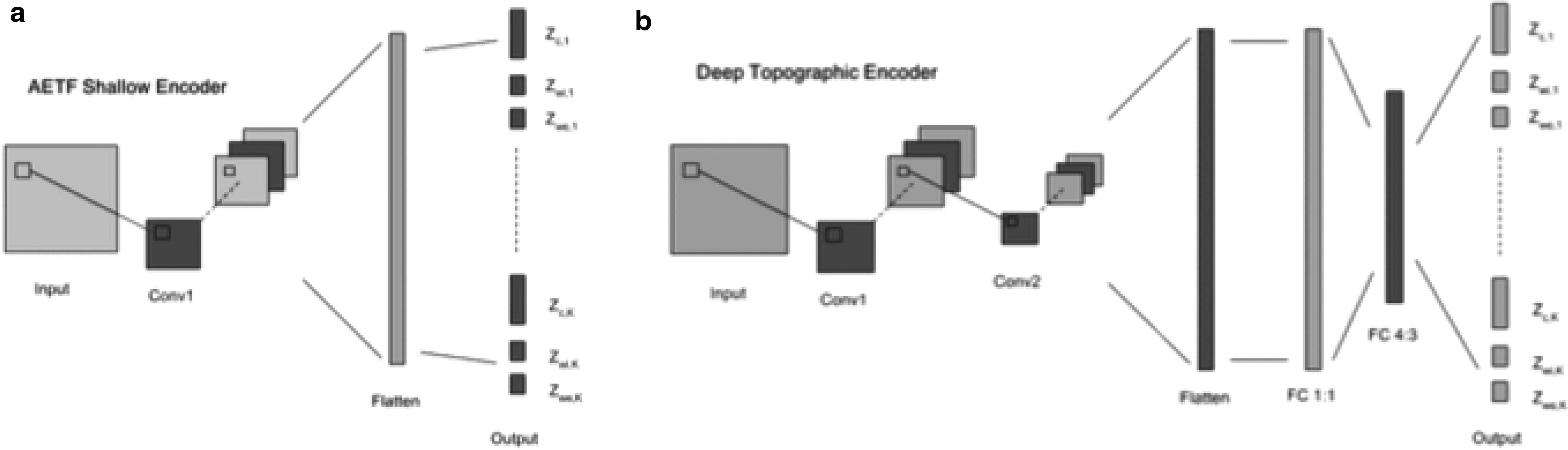
We generate a synthetic data set using \documentclass{aastex}\usepackage{amsbsy}\usepackage{amsfonts}\usepackage{amssymb}\usepackage{bm}\usepackage{mathrsfs}\usepackage{pifont}\usepackage{stmaryrd}\usepackage{textcomp}\usepackage{portland, xspace}\usepackage{amsmath, amsxtra}\usepackage{upgreek}\pagestyle{empty}\DeclareMathSizes{10}{9}{7}{6}\begin{document}
$$k = 2$$
\end{document} source functions over 1000 observations on a 20 × 20 × 20 lattice. In our experiments, TFA was unable to handle larger lattice dimensions in \documentclass{aastex}\usepackage{amsbsy}\usepackage{amsfonts}\usepackage{amssymb}\usepackage{bm}\usepackage{mathrsfs}\usepackage{pifont}\usepackage{stmaryrd}\usepackage{textcomp}\usepackage{portland, xspace}\usepackage{amsmath, amsxtra}\usepackage{upgreek}\pagestyle{empty}\DeclareMathSizes{10}{9}{7}{6}\begin{document}
$${ \mathbb{R}^3}$$
\end{document}. Unlike the generative process specified in TFA (Manning et al., 2014a), the position of each source function may shift across observations and is not restricted to be collocated on the lattice. This design choice is relevant given that the blood oxygen level dependency response is not static and often transforms dynamically as a time series. Figure 2a provides a schematic illustrating the position of two sources located near the vertices of the cube. Each source function is permitted to drift between one of two possible states, which are represented using the red and black colors. Figure 2b and c provides the variance explained on the training and testing sets, respectively, using \documentclass{aastex}\usepackage{amsbsy}\usepackage{amsfonts}\usepackage{amssymb}\usepackage{bm}\usepackage{mathrsfs}\usepackage{pifont}\usepackage{stmaryrd}\usepackage{textcomp}\usepackage{portland, xspace}\usepackage{amsmath, amsxtra}\usepackage{upgreek}\pagestyle{empty}\DeclareMathSizes{10}{9}{7}{6}\begin{document}
$$k = 2$$
\end{document} components. TFA, independent component analysis (ICA), and principal component analysis (PCA) underperform relative to DL and AETF. Unlike DL, AETF is able to parameterize the transforming source functions while maintaining nearly all of the variances explained.
Description of the first simulation: (a) schematic illustrating two source functions located near the vertices of the lattice. Each source transforms across observations drifting between one of two states (denoted with shades light and darker); (b) variance explained for different models using two components. AETF outperforms TFA on the train set; (c) TFA, PCA, and ICA underperform on the test set. ICA, independent components analysis, PCA, principal components analysis; TFA, topographic factor analysis.
4.2. Gaussian random fields
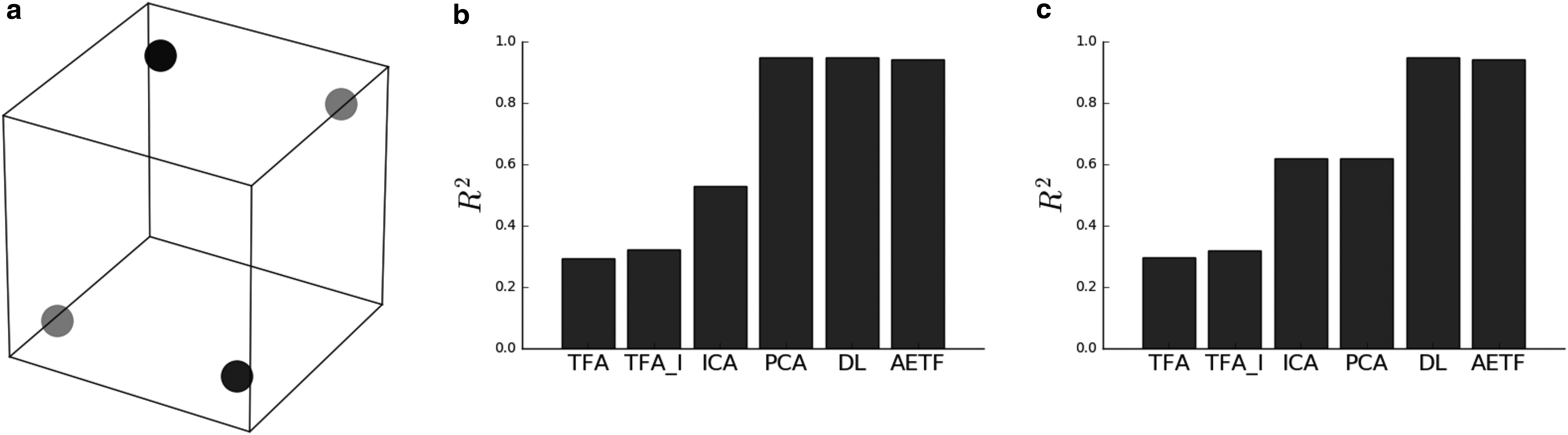
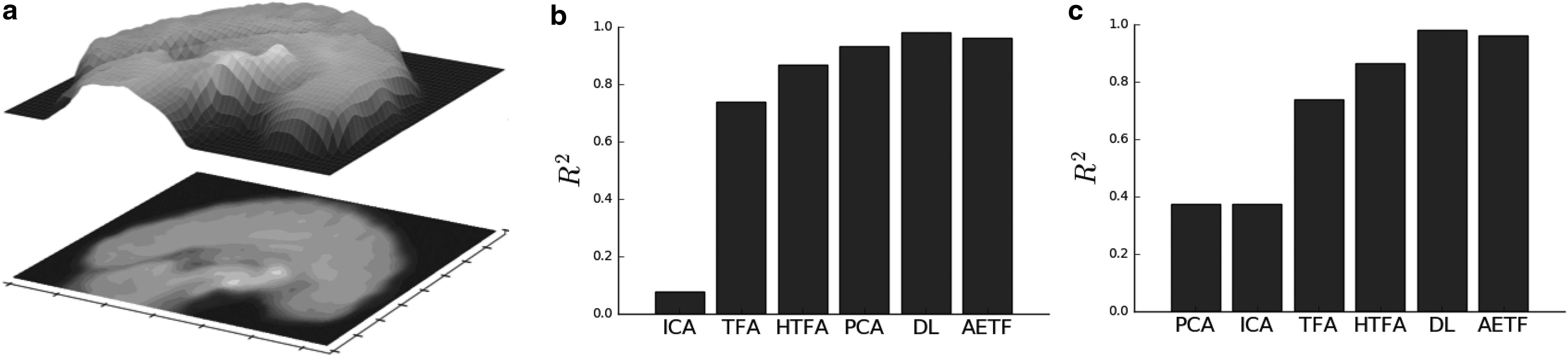
Gaussian random fields (GRFs) are often used in image analysis to model stochastic processes on a lattice and to introduce noise. We illustrate how AETF recovers autocorrelation structure by filtering a sequence of GRFs simulated using spectral methods (Annika and Jrgen, 2011). The spectral density of a fixed covariance kernel is multiplied with a Fourier transformed white noise field before applying an inverse transform. This process introduces a nonsmooth signal in which spatial autocorrelations are not explicitly collocated across observations. Figure 3a provides a representative sample along with the inferred reconstruction in Figure 3b. We fit 10 source functions to 1000 observations on a cubic lattice. As a visualization, the planar cross section is provided in Figure 3. The surface is shifted above the image to illustrate the smoothness of the field along with contours presenting the location of the inferred spatial factors. Figure 3c provides the variance explained across models and fits. AETF outperforms TFA, ICA, DL, and PCA; the canonical method for Gaussian data. It is clear that TFA underperforms when the correlation structure is not held fixed.
Summary of the AETF fit to the GRF simulation: (a) the cross section of a single observation and (b) the cross section of the AETF topographic reconstruction. The surface is shifted above the plane to illustrate the smoothness of the field along with contours presenting the location of the inferred spatial factors; (c) variance explained across models. AETF provides the highest R2. GRF, Gaussian random field.
4.2.1. Image noise
Spatial factor models learn a smooth statistical map in the presence of noise in which the desired signal extends over several lattice points. A good fit should be robust to variation between observations while preserving the correlation structure within the data. To achieve this, autoencoding topographic factors learns a unique decomposition by simultaneously factorizing the observation matrix, inferring the position of spatial dependencies, and introducing flexibility for the location of factors across the lattice. This process is analogous to blurring residual differences in location between comparable areas of activation. When two observations are similar, this is captured in their latent spatial representations. For heterogeneous data, AETF parameterizes spatial dynamics.
4.2.2. Initializing TFA and hierarchical TFA
Heuristics are often suggested to initialize hyperparameters for TFA so that local optima in the source image matrix do not serve as an impediment for nonconvex optimization. There exist multiple values of parameters for the location and width of the sources that are equally likely to have generated an observation \documentclass{aastex}\usepackage{amsbsy}\usepackage{amsfonts}\usepackage{amssymb}\usepackage{bm}\usepackage{mathrsfs}\usepackage{pifont}\usepackage{stmaryrd}\usepackage{textcomp}\usepackage{portland, xspace}\usepackage{amsmath, amsxtra}\usepackage{upgreek}\pagestyle{empty}\DeclareMathSizes{10}{9}{7}{6}\begin{document}
$${{ \bf{y}}_n}$$
\end{document}, due to the rotational invariance of F. One proposed approach is to place hyperparameters a-priori in locations corresponding to high and low activation. Hotspot initialization (Manning et al., 2014a) refers to an iterative process in which the mean image is computed, the mean activation is subtracted, and the absolute value is taken of all of the remaining activations. The result is an energy landscape in which peaks correspond to extremum. These peaks are iteratively flattened as source centers are placed on these extremum. Values for \documentclass{aastex}\usepackage{amsbsy}\usepackage{amsfonts}\usepackage{amssymb}\usepackage{bm}\usepackage{mathrsfs}\usepackage{pifont}\usepackage{stmaryrd}\usepackage{textcomp}\usepackage{portland, xspace}\usepackage{amsmath, amsxtra}\usepackage{upgreek}\pagestyle{empty}\DeclareMathSizes{10}{9}{7}{6}\begin{document}
$${{ \bf{m}}_{{s_{n , k}}}}$$
\end{document} the mean of the distribution for source \documentclass{aastex}\usepackage{amsbsy}\usepackage{amsfonts}\usepackage{amssymb}\usepackage{bm}\usepackage{mathrsfs}\usepackage{pifont}\usepackage{stmaryrd}\usepackage{textcomp}\usepackage{portland, xspace}\usepackage{amsmath, amsxtra}\usepackage{upgreek}\pagestyle{empty}\DeclareMathSizes{10}{9}{7}{6}\begin{document}
$$k{ \rm{ \prime }}s$$
\end{document} width scale are then solved via Newton's method. Once preinitialized, the source centers and width scales frequently remain fixed. In our experiments, sources for TFA initialized using both hotspot initialization and k-means outperformed experiments with no initialization. AETF outperformed both methods without being contingent on any such initialization to perform inference successfully.
4.3. NYU data set
We consider the problem of modeling functional images using the NYU test–retest data set (Shehzad et al., 2009). Data were obtained using a Siemens Allegra 3.0 Tesla scanner. Data consist of 26 participants each with 3 resting-state scans of 197 continuous EPI functional volumes. Each scan consists of 39 slices of a matrix \documentclass{aastex}\usepackage{amsbsy}\usepackage{amsfonts}\usepackage{amssymb}\usepackage{bm}\usepackage{mathrsfs}\usepackage{pifont}\usepackage{stmaryrd}\usepackage{textcomp}\usepackage{portland, xspace}\usepackage{amsmath, amsxtra}\usepackage{upgreek}\pagestyle{empty}\DeclareMathSizes{10}{9}{7}{6}\begin{document}
$$64 \times 64$$
\end{document} with an acquisition voxel size of \documentclass{aastex}\usepackage{amsbsy}\usepackage{amsfonts}\usepackage{amssymb}\usepackage{bm}\usepackage{mathrsfs}\usepackage{pifont}\usepackage{stmaryrd}\usepackage{textcomp}\usepackage{portland, xspace}\usepackage{amsmath, amsxtra}\usepackage{upgreek}\pagestyle{empty}\DeclareMathSizes{10}{9}{7}{6}\begin{document}
$$3 \times 3 \times 3$$
\end{document} mm. Scans 2 and 3 were conducted 45 minutes apart roughly 5–16 months after Scan 1.
Slice timing correction, spatial normalization, smoothing, and noise stripping were performed using the Nipype interface to the FSL software library. The sequential dependency of the time series was not accommodated and each time frame was treated independently. An AETF model was trained using all three sessions reserving 20% for the testing set as a performance criteria to evaluate our fit. To test the significance of the lattice dimensions, models were fit to both sagittal cross-section data and full cubic volumes.
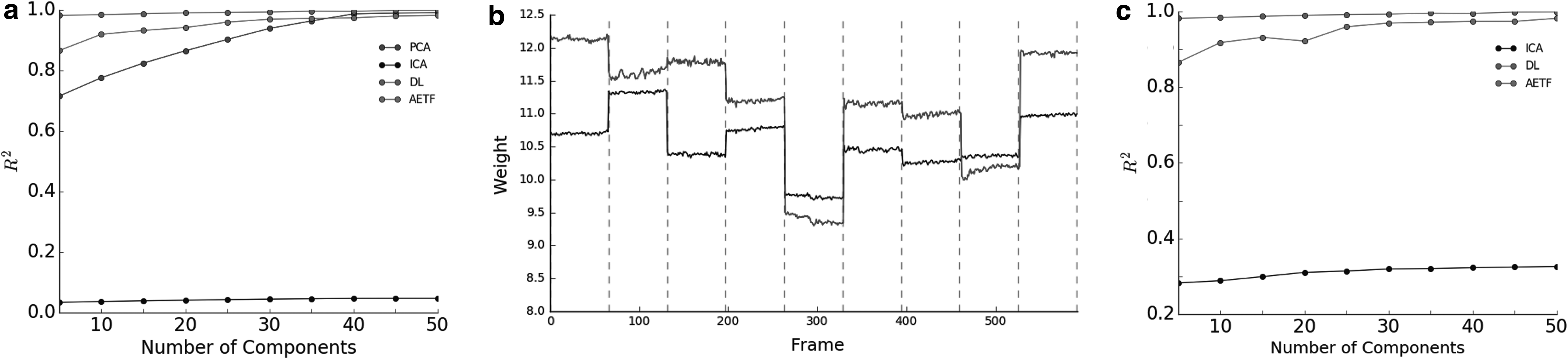
4.3.1. Sagittal cross sections in 2D
Sagittal cross-section data were fit to the 13 subjects using the first session. Figure 4a provides the variance explained for AETF, PCA, ICA, and DL as a function of number of sources on training data. TFA and hierarchical TFA (HTFA) implementations are not supported on the 2D lattice. The R2 approaches 1 the number of sources K increases. Figure 4b plots the weight values for two randomly selected source functions across a subset of time frames. Dashed vertical lines distinguish subjects. Strong per-subject similarities are visible. Figure 4c provides the variance explained by AETF as K increases on the test data. Using \documentclass{aastex}\usepackage{amsbsy}\usepackage{amsfonts}\usepackage{amssymb}\usepackage{bm}\usepackage{mathrsfs}\usepackage{pifont}\usepackage{stmaryrd}\usepackage{textcomp}\usepackage{portland, xspace}\usepackage{amsmath, amsxtra}\usepackage{upgreek}\pagestyle{empty}\DeclareMathSizes{10}{9}{7}{6}\begin{document}
$$k = 50$$
\end{document} source functions, 99% of variance is explained. We find that \documentclass{aastex}\usepackage{amsbsy}\usepackage{amsfonts}\usepackage{amssymb}\usepackage{bm}\usepackage{mathrsfs}\usepackage{pifont}\usepackage{stmaryrd}\usepackage{textcomp}\usepackage{portland, xspace}\usepackage{amsmath, amsxtra}\usepackage{upgreek}\pagestyle{empty}\DeclareMathSizes{10}{9}{7}{6}\begin{document}
$$K = 25$$
\end{document} anisotropic sources are sufficient for high-quality reconstruction. Interestingly, AETF is able to converge without any preprocessing to preserve 89% of total variance on the raw NYU data. On the preprocessed data set, 25 source functions preserve 98% of total variance.
Summary of the sagittal cross-section NYU data: (a) variance explained for various models as a function of number of sources on the training data; (b) two source weights plotted across time frames illustrating strong subject-specific similarities. Dashed vertical lines denote unique subjects; (c) variance explained as a function of number of sources for test data. AETF returns a near perfect variance explained using \documentclass{aastex}\usepackage{amsbsy}\usepackage{amsfonts}\usepackage{amssymb}\usepackage{bm}\usepackage{mathrsfs}\usepackage{pifont}\usepackage{stmaryrd}\usepackage{textcomp}\usepackage{portland, xspace}\usepackage{amsmath, amsxtra}\usepackage{upgreek}\pagestyle{empty}\DeclareMathSizes{10}{9}{7}{6}\begin{document}
$$k = 25$$
\end{document} source functions.
4.3.2. Functional imaging with 3D volumes
The three-session NYU data on the cubic lattice were modeled using AETF, TFA, and HTFA. The \documentclass{aastex}\usepackage{amsbsy}\usepackage{amsfonts}\usepackage{amssymb}\usepackage{bm}\usepackage{mathrsfs}\usepackage{pifont}\usepackage{stmaryrd}\usepackage{textcomp}\usepackage{portland, xspace}\usepackage{amsmath, amsxtra}\usepackage{upgreek}\pagestyle{empty}\DeclareMathSizes{10}{9}{7}{6}\begin{document}
$$64 \times 64 \times 40$$
\end{document} lattice was divided into eight \documentclass{aastex}\usepackage{amsbsy}\usepackage{amsfonts}\usepackage{amssymb}\usepackage{bm}\usepackage{mathrsfs}\usepackage{pifont}\usepackage{stmaryrd}\usepackage{textcomp}\usepackage{portland, xspace}\usepackage{amsmath, amsxtra}\usepackage{upgreek}\pagestyle{empty}\DeclareMathSizes{10}{9}{7}{6}\begin{document}
$$20 \times 20 \times 20$$
\end{document} cubic volumes. TFA and HTFA were unable to handle larger lattice dimensions on the full set of 7683 frames. We fit \documentclass{aastex}\usepackage{amsbsy}\usepackage{amsfonts}\usepackage{amssymb}\usepackage{bm}\usepackage{mathrsfs}\usepackage{pifont}\usepackage{stmaryrd}\usepackage{textcomp}\usepackage{portland, xspace}\usepackage{amsmath, amsxtra}\usepackage{upgreek}\pagestyle{empty}\DeclareMathSizes{10}{9}{7}{6}\begin{document}
$$k = 10$$
\end{document} source functions to each cubic volume and average the cost across the total area. For TFA, one model was fit across subjects, whereas 39 subjects were fit using HTFA. Figure 7a displays a new frame evaluated using the trained model to illustrate the effect of applying the trained model on unseen data. The surface is plotted above the image to highlight the areas of activation above the corresponding factors on the mesh. Figure 7a and b provides the train and test R2, respectively. It is clear that AETF outperforms both methods. Unlike HTFA, the hierarchical covariance structure is inferred from the data and not specified a-priori.
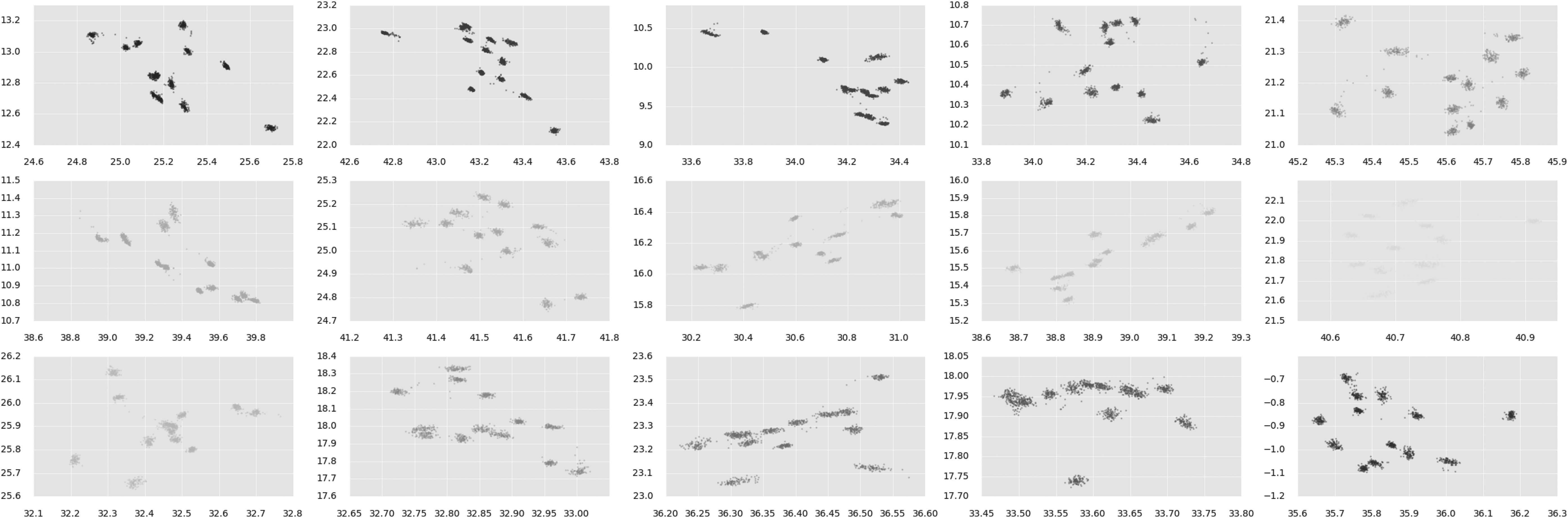
The distribution of the top 15 weighted source center means for subjects and time frames. Colors represent distinct source function center means. The outline of a single frame is provided as a reference. Each point is a parameter for an image in a collection of time series. The latent factors recovered by AETF exhibit strong spatial localization.
The distribution of center means enhanced for each individual source function. Factors are distinguished by color matching their corresponding representations in Figure 5. Each point is a parameter for an image in a collection of time series. Thirteen clusters appear consistently within each factor recovering the number of subjects. AETF latent representations implicitly preserve hierarchical covariance structure and can be used for clustering.
Results for the cubic volume NYU data: (a) a cross section of a frame and the surface highlighting source intensities; R2 values for training (b) and testing (c) for various models averaged across eight cubic volumes using \documentclass{aastex}\usepackage{amsbsy}\usepackage{amsfonts}\usepackage{amssymb}\usepackage{bm}\usepackage{mathrsfs}\usepackage{pifont}\usepackage{stmaryrd}\usepackage{textcomp}\usepackage{portland, xspace}\usepackage{amsmath, amsxtra}\usepackage{upgreek}\pagestyle{empty}\DeclareMathSizes{10}{9}{7}{6}\begin{document}
$$k = 10$$
\end{document} source functions. AETF consistently outperforms both TFA and HTFA. TFA, topographic factor analysis; HTFA, hierarchical topographic factor analysis.
5. Discussion
In the context of functional imaging, a spatial model should be able to extract both global and individual characteristics. In examining how the model parameters for centers, widths, and weights varied across testing data, we find source centers are not only similar at the per-subject microscale but also marginally similar at the global macroscale. However, we see much more global variability with weight values. Compared with a similar factorization in Manning et al. (2014b) that constricts learning to globally shared sources and individual per-frame weights, our model naturally learns a similar representation. Namely, through a shared encoder mapping, source variability is less pronounced than weight variability.
AETF offers several advantages over unstructured blind source separation techniques. TFA, HTFA, DL, PCA, and ICA explicitly learn factor weights (loadings) for each observation. The number of trainable parameters is therefore linear with respect to N, the number of observations. AETF parameters φ are constant with respect to N. This paradigm reduces memory footprint for large N and allows AETF to handle unseen data. By design, the factor images learned by AETF possess lower complexity than the observed images.
AETF can accommodate any priors but is not contingent on an a-priori choice of generative model hyperparameters to converge. This is mitigated by choosing uniform priors for the generative model. In this way, AETF is not sensitive to preinitialization issues that plague TFA and HTFA. It is also possible to parameterize the priors of the generative model using a trainable decoder network. Unlike TFA and HTFA, source functions are allowed to transform across individual frames. This is advantageous for time series modeling. In our experiments, DL sometimes provided a comparable R2. AETF, however, returns a factorization along with spatially parameterized functions. AETF was written in TensorFlow. The source code and several visualizations are available online.
6. Conclusions
We have presented AETF, a novel variational inference scheme, for lattice-based measurements in which each observation is given a unique spatial decomposition. The proposed method is robust to high-dimensional data in which sources are not rigidly collocated, introduces nonlinearity, supports a family of kernels, and the ability to enforce a constrained or non-negative matrix factorization. AETF preserves a large proportion of variance even when factor positions shift dynamically across observations. Highlights include the ability to identify autocorrelation structure in a collection of random fields and the ability to scale to thousands of 3D functional images with a number of training parameters independent of data set size.
The results, in particular Figure 4b, motivate an explicitly hierarchical AETF across individuals, as well as a temporally correlated AETF. A natural extension is to explore the method of normalizing flows (Rezende and Mohamed, 2015; Kingma et al., 2016) as an alternative to defining factors by specifying kernels for source functions. We expect that the approximate posterior would remain simple to compute while each source is permitted to undergo a sequence of transformations giving rise to complex and expressive spatial dependencies.
Footnotes
Author Disclosure Statement
The authors declare that no competing financial interests exist.
References
1.
AnnikaL., and JrgenP.2011. Fast simulation of gaussian random fields. Monte Carlo Methods Appl. 17, 195–214.
2.
CandèsE.J., LiX., MaY., et al.2011. Robust principal component analysis?. J. ACM, 58, 11:1–11:37.
3.
GershmanS., BleiD.M., PereiraF., et al.2011. A topographic latent source model for fmri data. Neuroimage, 57, 89–100.
4.
GershmanS., BleiD.M., NormanK.A., et al.2014. Decomposing spatiotemporal brain patterns into topographic latent sources. Neuroimage, 98, 91–102.
5.
FriedrichJ., SoudryD., MuY., et al.2015. Fast constrained non-negative matrix factorization for whole-brain calcium imaging data. In NIPS Workshop on Statistical Methods for Understanding Neural Systems.
6.
KingmaD.P., and BaJ.2015. Adam: A method for stochastic optimization. In 3rd International Conference for Learning Representations, San Diego.
7.
KingmaD.P., and WellingM.2013. Auto-encoding variational bayes. CoRR, abs/1312.6114, 2013.
8.
KingmaD.P., SalimansT., JózefowiczR., et al.2016. Improving variational autoencoders with inverse autoregressive flow. In NIPS, 4736–4744.
9.
LeeD.D., and SeungS.H.2001. Algorithms for non-negative matrix factorization, 556–562. In LeenT.K., DietterichT.G., and TrespV., eds. Advances in Neural Information Processing Systems, Vol. 13. MIT Press.
10.
LiangD., KrishnanR., HoffmanM., et al.2018. Variational autoencoders for collaborative filtering. In Proceedings of The Web Conference (WWW), 2018, 2018.
ManningJ.R., RanganathR., KeungW., et al.2014a. Hierarchical topographic factor analysis, 1–4. In International Workshop on Pattern Recognition in Neuroimaging, PRNI 2014, Tübingen, Germany, June 4–6, 2014. DOI: 10.1109/PRNI.2014.6858530
13.
ManningJ.R., RanganathR., NormanK.A., et al.2014b. Topographic factor analysis: A Bayesian Model for inferring brain networks from neural data. PLoS ONE, 9, e94914.
14.
MukamelE.A, NimmerjahnA., and SchnitzerM.J.2009. Automated analysis of cellular signals from large-scale calcium imaging data. Neuron, 63, 747–760.
15.
PnevmatikakisE.A., SoudryD., GaoY., et al.2016. Simultaneous denoising, deconvolution, and demixing of calcium imaging data. Neuron, 89, 285–299.
16.
RanganathR., GerrishS., and BleiD.M.2014. Black box variational inference, 814–822. In Proceedings of the Seventeenth International Conference on Artificial Intelligence and Statistics, AISTATS, Reykjavik, Iceland, April 22–25, 2014.
17.
RezendeD.J., and MohamedS.2015. Variational inference with normalizing flows, 1530–1538. In Proceedings of the 32nd International Conference on Machine Learning, ICML 2015, Lille, France, July 6–11, 2015.
18.
RezendeD.J., MohamedS., and WierstraD.2014. Stochastic backpropagation and approximate inference in deep generative models, 1278–1286. In XingEP., and JebaraT., eds. Proceedings of the 31st International Conference on Machine Learning, volume 32 of Proceedings of Machine Learning Research (PMLR), Bejing, China, June 22–24, 2014.
19.
ShehzadZ., KellyA.M., ClareR., et al.2009. The resting brain: Unconstrained yet reliable. Cereb Cortex. 19, 2209–2229.
20.
SvenssonV., TeichmannS.A., and StegleO.2017. SpatialDE—Identification of spatially variable genes. bioRxiv, 143321, May 2017. DOI: 10.1101/143321.
21.
WorsleyK.J., MarrettS., NeelinP., et al.1996. A unified statistical approach for determining significant signals in location and scale space images of cerebral activation.