Identifying individual characteristics is a crucial issue in personalized genome research. To effectively identify sample-specific characteristics, we propose a novel strategy called robust sample-specific stability selection. Although stability selection shows effective feature selection results and has attractive theoretical property (i.e., per-family error rate control), the method's results are sensitive to the value of the regularization parameter because the method performs feature selection based only on the particular parameter value that maximizes the selection probability. To resolve this issue, we propose robust stability selection and show that our method provides an effective theoretical property (i.e., effective per-family error rate control). We also propose a sample-specific random lasso based on the kernel-based L1-type regularization and weighted random sampling. The proposed robust sample-specific stability selection estimates the selection probabilities of variables using the sample-specific random lasso and then selects variables based on robust stability selection. Our method controls the effect of samples on sample-specific analysis by the two-stage strategy (i.e., the weighted random sampling and the kernel-based L1-type approach in the random lasso), and thus we can effectively perform sample-specific analysis without disturbances of samples having characteristics different from those of the target sample. We observe from the numerical studies that our strategies can effectively perform sample-specific analysis and provide biologically reliable results in gene selection.
1. Introduction
Currently, patient (sample)-specific analysis has drawn a large amount of attention for identifying individual molecular characteristics in the progression of cancer. Although various L1-type regularization approaches [elastic nets, ELAs (Zou and Hastie, 2005), etc.] have been widely used for high-dimensional genomic data analysis, the existing methods provide averaged results for all samples. Thus, we cannot identify patient-specific molecular characteristics by using the existing L1-type regularization methods.
To resolve the issue, Shimamura et al. (2011) proposed a kernel-based L1-type regularization method, called NetworkProfiler (NP). By using the Gaussian kernel function, this method groups samples according to their characteristics and then constructs the gene network for a target sample based only on the neighboring samples around the target sample. It was demonstrated, however, that the existing L1-type regularization methods used in NP [e.g., the lasso (Tibshirani, 1996) and the ELA] provide erroneous modeling results in the presence of multicollinearity between variables (Wang et al., 2011).
To effectively identify sample-specific molecular mechanisms, we propose a novel sample-specific stability selection method based on the random lasso procedure (Wang et al., 2011). For a regularization parameter \documentclass{aastex}\usepackage{amsbsy}\usepackage{amsfonts}\usepackage{amssymb}\usepackage{bm}\usepackage{mathrsfs}\usepackage{pifont}\usepackage{stmaryrd}\usepackage{textcomp}\usepackage{portland, xspace}\usepackage{amsmath, amsxtra}\usepackage{upgreek}\pagestyle{empty}\DeclareMathSizes{10}{9}{7}{6}\begin{document}
$$\lambda \in \Lambda$$
\end{document}, stability selection (Meinshausen and Bühlmann, 2010) computes the selection probability of each feature and then performs feature selection based on the maximum value of the selection probability for \documentclass{aastex}\usepackage{amsbsy}\usepackage{amsfonts}\usepackage{amssymb}\usepackage{bm}\usepackage{mathrsfs}\usepackage{pifont}\usepackage{stmaryrd}\usepackage{textcomp}\usepackage{portland, xspace}\usepackage{amsmath, amsxtra}\usepackage{upgreek}\pagestyle{empty}\DeclareMathSizes{10}{9}{7}{6}\begin{document}
$$\lambda \in \Lambda$$
\end{document}. However, the use of the maximum value of the selection probability may lead to modeling results that are extremely sensitive to the regularization parameter because a selected variable may have a high probability only for a particular value of the regularization parameter. This property implies that ordinary stability selection based on the maximum value of the selection probability may lead to false positive results in feature selection.
To settle the issue, we propose robust stability selection, which performs feature selection based not on a particular parameter value but rather on all of the parameter values. Thus, our method does not suffer from the drawback of ordinary stability selection that a selected variable may have a high selection probability for only a particular value of the parameter. Furthermore, we demonstrate an effective theoretical property of the proposed robust stability selection in line with top-K stability selection (Zhou et al., 2013), that is, the upper bound of the expected number of falsely selected variables of our method is guaranteed to be smaller than that of the ordinary stability selection method. We then propose robust sample-specific stability selection based on a sample-specific random lasso and robust stability selection. In our method, the effect of samples on sample-specific analysis is controlled by a two-stage strategy, that is, weighted bootstrap sampling and kernel-based L1-type regularized regression modeling in a sample-specific random lasso. Thus, we can effectively perform sample-specific analysis without disturbances of samples having a characteristic different from that of the target sample.
The effectiveness of our method is investigated through Monte Carlo simulations. We also apply the proposed method to the publicly available Sanger Genomic of Drug Sensitivity in Cancer data set from the Cancer Genome Project (www.cancerrxgene.org/), and we construct gene networks specific to anticancer drug sensitivities. Through the numerical analysis, we can see that the proposed strategy performs effectively for sample-specific analysis and provides biologically reliable results in gene selection.
The rest of this article is organized as follows. In Section 2, we explain the existing method for sample-specific analysis with a particular focus on NP. We propose robust sample-specific stability selection in Section 3; Section 7 proves the theoretical properties of robust stability selection. In Section 4, Monte Carlo simulations are conducted to investigate the effectiveness of the proposed strategy. We apply the proposed method to construct a drug sensitivity-specific gene network in Section 5. Some conclusions are given in Section 6.
2. Existing Methods for Sample-Specific Analysis
Suppose \documentclass{aastex}\usepackage{amsbsy}\usepackage{amsfonts}\usepackage{amssymb}\usepackage{bm}\usepackage{mathrsfs}\usepackage{pifont}\usepackage{stmaryrd}\usepackage{textcomp}\usepackage{portland, xspace}\usepackage{amsmath, amsxtra}\usepackage{upgreek}\pagestyle{empty}\DeclareMathSizes{10}{9}{7}{6}\begin{document}
$${R_1} , \ldots , {R_p}$$
\end{document} are p possible regulators that control transcription of the \documentclass{aastex}\usepackage{amsbsy}\usepackage{amsfonts}\usepackage{amssymb}\usepackage{bm}\usepackage{mathrsfs}\usepackage{pifont}\usepackage{stmaryrd}\usepackage{textcomp}\usepackage{portland, xspace}\usepackage{amsmath, amsxtra}\usepackage{upgreek}\pagestyle{empty}\DeclareMathSizes{10}{9}{7}{6}\begin{document}
$${l^{{ \rm{th}}}}$$
\end{document} target gene Tl. Consider the varying coefficient model,
\documentclass{aastex}\usepackage{amsbsy}\usepackage{amsfonts}\usepackage{amssymb}\usepackage{bm}\usepackage{mathrsfs}\usepackage{pifont}\usepackage{stmaryrd}\usepackage{textcomp}\usepackage{portland, xspace}\usepackage{amsmath, amsxtra}\usepackage{upgreek}\pagestyle{empty}\DeclareMathSizes{10}{9}{7}{6}\begin{document}
\begin{align*}
{T_l} = \sum \limits_{j = 0}^p { \beta _{jl}} ( {m_ \alpha } ) \cdot {R_j} + { \varepsilon _l} , \quad \alpha = 1 , \ldots , n , \tag{1}
\end{align*}
\end{document}
where \documentclass{aastex}\usepackage{amsbsy}\usepackage{amsfonts}\usepackage{amssymb}\usepackage{bm}\usepackage{mathrsfs}\usepackage{pifont}\usepackage{stmaryrd}\usepackage{textcomp}\usepackage{portland, xspace}\usepackage{amsmath, amsxtra}\usepackage{upgreek}\pagestyle{empty}\DeclareMathSizes{10}{9}{7}{6}\begin{document}
$${ \beta _{jl}} ( {m_ \alpha } )$$
\end{document} is a regression coefficient of the jth regulator on the lth target gene for the \documentclass{aastex}\usepackage{amsbsy}\usepackage{amsfonts}\usepackage{amssymb}\usepackage{bm}\usepackage{mathrsfs}\usepackage{pifont}\usepackage{stmaryrd}\usepackage{textcomp}\usepackage{portland, xspace}\usepackage{amsmath, amsxtra}\usepackage{upgreek}\pagestyle{empty}\DeclareMathSizes{10}{9}{7}{6}\begin{document}
$$\alpha th$$
\end{document} sample, which has a modulator value \documentclass{aastex}\usepackage{amsbsy}\usepackage{amsfonts}\usepackage{amssymb}\usepackage{bm}\usepackage{mathrsfs}\usepackage{pifont}\usepackage{stmaryrd}\usepackage{textcomp}\usepackage{portland, xspace}\usepackage{amsmath, amsxtra}\usepackage{upgreek}\pagestyle{empty}\DeclareMathSizes{10}{9}{7}{6}\begin{document}
$$M = {m_ \alpha }$$
\end{document} that indicates a specific characteristic of a sample, such as the response of patients to a drug. To estimate the varying coefficients, Shimamura et al. (2011) proposed a novel kernel-based regularization method, called NP, as follows:
\documentclass{aastex}\usepackage{amsbsy}\usepackage{amsfonts}\usepackage{amssymb}\usepackage{bm}\usepackage{mathrsfs}\usepackage{pifont}\usepackage{stmaryrd}\usepackage{textcomp}\usepackage{portland, xspace}\usepackage{amsmath, amsxtra}\usepackage{upgreek}\pagestyle{empty}\DeclareMathSizes{10}{9}{7}{6}\begin{document}
\begin{align*}
L ( { \beta _ { l \alpha } } \vert { h_l } ) = \frac { 1 } { 2 } \sum \limits_ { i = 1 } ^n { ( { t_ { il } } - \sum \limits_ { j = 1 } ^p { \beta _ { jl \alpha } } { r_ { ij } } ) ^2 } G ( { m_i } - { m_ \alpha } \vert { h_l } ) + { P_ { { \delta _ { l \alpha } } { \lambda _ { l \alpha } } } } ( { \beta _ { l \alpha } } ) , \tag { 2 }
\end{align*}
\end{document}
where \documentclass{aastex}\usepackage{amsbsy}\usepackage{amsfonts}\usepackage{amssymb}\usepackage{bm}\usepackage{mathrsfs}\usepackage{pifont}\usepackage{stmaryrd}\usepackage{textcomp}\usepackage{portland, xspace}\usepackage{amsmath, amsxtra}\usepackage{upgreek}\pagestyle{empty}\DeclareMathSizes{10}{9}{7}{6}\begin{document}
$${w_{jl \alpha }} = 1 / ( \vert { \tilde \beta _{jl \alpha }} \vert + \xi )$$
\end{document} (\documentclass{aastex}\usepackage{amsbsy}\usepackage{amsfonts}\usepackage{amssymb}\usepackage{bm}\usepackage{mathrsfs}\usepackage{pifont}\usepackage{stmaryrd}\usepackage{textcomp}\usepackage{portland, xspace}\usepackage{amsmath, amsxtra}\usepackage{upgreek}\pagestyle{empty}\DeclareMathSizes{10}{9}{7}{6}\begin{document}
$${ \tilde \beta _{jl \alpha }}$$
\end{document} is estimated coefficient from the previous step) and \documentclass{aastex}\usepackage{amsbsy}\usepackage{amsfonts}\usepackage{amssymb}\usepackage{bm}\usepackage{mathrsfs}\usepackage{pifont}\usepackage{stmaryrd}\usepackage{textcomp}\usepackage{portland, xspace}\usepackage{amsmath, amsxtra}\usepackage{upgreek}\pagestyle{empty}\DeclareMathSizes{10}{9}{7}{6}\begin{document}
$$G ( {m_i} - {m_ \alpha } \vert {h_l} )$$
\end{document} is the Gaussian kernel function with a bandwidth hl,
The Gaussian kernel function \documentclass{aastex}\usepackage{amsbsy}\usepackage{amsfonts}\usepackage{amssymb}\usepackage{bm}\usepackage{mathrsfs}\usepackage{pifont}\usepackage{stmaryrd}\usepackage{textcomp}\usepackage{portland, xspace}\usepackage{amsmath, amsxtra}\usepackage{upgreek}\pagestyle{empty}\DeclareMathSizes{10}{9}{7}{6}\begin{document}
$$G ( {m_i} - {m_ \alpha } \vert {h_l} )$$
\end{document} is used to group samples according to the modulator (e.g., a specific cancer characteristic of samples), and thus we can perform modeling for the \documentclass{aastex}\usepackage{amsbsy}\usepackage{amsfonts}\usepackage{amssymb}\usepackage{bm}\usepackage{mathrsfs}\usepackage{pifont}\usepackage{stmaryrd}\usepackage{textcomp}\usepackage{portland, xspace}\usepackage{amsmath, amsxtra}\usepackage{upgreek}\pagestyle{empty}\DeclareMathSizes{10}{9}{7}{6}\begin{document}
$$\alpha th$$
\end{document} target sample based only on samples that have a characteristic similar to that of the target sample. However, the L1-type approaches used in NP suffer from the following drawbacks (Wang et al., 2011; Park et al., 2015):
Lasso: The lasso cannot account for the grouping effect of predictor variables in regression modeling, and thus tends to choose only one or a few of the variables among highly correlated variables even though all are related to a response variable.
ELA: The grouping effect of the ELA leads to erroneous estimation results when the coefficients of highly correlated variables have different magnitudes and, particularly, when they have different signs.
This finding implies that NP also suffers from the mentioned drawbacks. To resolve the issues and improve the accuracy of feature selection in sample-specific analysis, we propose a novel strategy, called robust sample-specific stability selection based on the random lasso, which can overcome the drawbacks of the existing L1-type methods (i.e., multicollinearity) by using the random forest method (Wang et al., 2011).
3. Robust Sample-Specific Stability Selection
3.1. Stability selection
Meinshausen and Bühlmann (2010) proposed stability selection, which is based on aggregating the results of a variable selection procedure (a lasso, an ELA, etc.) for subsamples of data.
Denote the sets of active and noise variables as \documentclass{aastex}\usepackage{amsbsy}\usepackage{amsfonts}\usepackage{amssymb}\usepackage{bm}\usepackage{mathrsfs}\usepackage{pifont}\usepackage{stmaryrd}\usepackage{textcomp}\usepackage{portland, xspace}\usepackage{amsmath, amsxtra}\usepackage{upgreek}\pagestyle{empty}\DeclareMathSizes{10}{9}{7}{6}\begin{document}
$$S = \{ j;{ \beta _j} \ne 0 \} $$
\end{document} and \documentclass{aastex}\usepackage{amsbsy}\usepackage{amsfonts}\usepackage{amssymb}\usepackage{bm}\usepackage{mathrsfs}\usepackage{pifont}\usepackage{stmaryrd}\usepackage{textcomp}\usepackage{portland, xspace}\usepackage{amsmath, amsxtra}\usepackage{upgreek}\pagestyle{empty}\DeclareMathSizes{10}{9}{7}{6}\begin{document}
$$N = \{ j;{ \beta _j} = 0 \} $$
\end{document}, respectively. Let I be a random subsample of \documentclass{aastex}\usepackage{amsbsy}\usepackage{amsfonts}\usepackage{amssymb}\usepackage{bm}\usepackage{mathrsfs}\usepackage{pifont}\usepackage{stmaryrd}\usepackage{textcomp}\usepackage{portland, xspace}\usepackage{amsmath, amsxtra}\usepackage{upgreek}\pagestyle{empty}\DeclareMathSizes{10}{9}{7}{6}\begin{document}
$$\{ 1 , 2 , \ldots , n \} $$
\end{document} of size \documentclass{aastex}\usepackage{amsbsy}\usepackage{amsfonts}\usepackage{amssymb}\usepackage{bm}\usepackage{mathrsfs}\usepackage{pifont}\usepackage{stmaryrd}\usepackage{textcomp}\usepackage{portland, xspace}\usepackage{amsmath, amsxtra}\usepackage{upgreek}\pagestyle{empty}\DeclareMathSizes{10}{9}{7}{6}\begin{document}
$$\left\lfloor {n / 2} \right\rfloor$$
\end{document} drawn without replacement, where \documentclass{aastex}\usepackage{amsbsy}\usepackage{amsfonts}\usepackage{amssymb}\usepackage{bm}\usepackage{mathrsfs}\usepackage{pifont}\usepackage{stmaryrd}\usepackage{textcomp}\usepackage{portland, xspace}\usepackage{amsmath, amsxtra}\usepackage{upgreek}\pagestyle{empty}\DeclareMathSizes{10}{9}{7}{6}\begin{document}
$$\left\lfloor a \right\rfloor$$
\end{document} denotes the largest integer \documentclass{aastex}\usepackage{amsbsy}\usepackage{amsfonts}\usepackage{amssymb}\usepackage{bm}\usepackage{mathrsfs}\usepackage{pifont}\usepackage{stmaryrd}\usepackage{textcomp}\usepackage{portland, xspace}\usepackage{amsmath, amsxtra}\usepackage{upgreek}\pagestyle{empty}\DeclareMathSizes{10}{9}{7}{6}\begin{document}
$$\le a$$
\end{document}. For L1-type regularized regression modeling, the regularization parameter \documentclass{aastex}\usepackage{amsbsy}\usepackage{amsfonts}\usepackage{amssymb}\usepackage{bm}\usepackage{mathrsfs}\usepackage{pifont}\usepackage{stmaryrd}\usepackage{textcomp}\usepackage{portland, xspace}\usepackage{amsmath, amsxtra}\usepackage{upgreek}\pagestyle{empty}\DeclareMathSizes{10}{9}{7}{6}\begin{document}
$$\lambda \in \Lambda$$
\end{document} controls model complexity. Given the set of the regularization parameter values Λ, stability selection iteratively performs regression modeling for random subsets. For a given \documentclass{aastex}\usepackage{amsbsy}\usepackage{amsfonts}\usepackage{amssymb}\usepackage{bm}\usepackage{mathrsfs}\usepackage{pifont}\usepackage{stmaryrd}\usepackage{textcomp}\usepackage{portland, xspace}\usepackage{amsmath, amsxtra}\usepackage{upgreek}\pagestyle{empty}\DeclareMathSizes{10}{9}{7}{6}\begin{document}
$$\lambda \in \Lambda$$
\end{document}, we denote \documentclass{aastex}\usepackage{amsbsy}\usepackage{amsfonts}\usepackage{amssymb}\usepackage{bm}\usepackage{mathrsfs}\usepackage{pifont}\usepackage{stmaryrd}\usepackage{textcomp}\usepackage{portland, xspace}\usepackage{amsmath, amsxtra}\usepackage{upgreek}\pagestyle{empty}\DeclareMathSizes{10}{9}{7}{6}\begin{document}
$${ \hat S^ \lambda } ( {{ \bf{I}}_b} ) = \{ j: \hat \beta _j^b \ne 0 \} $$
\end{document} as a set of selected variables in the bth random subset. The regression modeling is repeated B times, and we compute the selection probability of each variable as follows:
\documentclass{aastex}\usepackage{amsbsy}\usepackage{amsfonts}\usepackage{amssymb}\usepackage{bm}\usepackage{mathrsfs}\usepackage{pifont}\usepackage{stmaryrd}\usepackage{textcomp}\usepackage{portland, xspace}\usepackage{amsmath, amsxtra}\usepackage{upgreek}\pagestyle{empty}\DeclareMathSizes{10}{9}{7}{6}\begin{document}
\begin{align*}
\hat \Pi _j^ \lambda = \frac { 1 } { B } \sum \limits_ { b = 1 }
^B { \bf { 1 } } \{ j \in { \hat S^ \lambda } ( { { \bf { I } } _b
} ) \} \quad { \rm { for } } \quad j = 1 , 2 , \ldots , p , \tag {
5 }
\end{align*}
\end{document}
where \documentclass{aastex}\usepackage{amsbsy}\usepackage{amsfonts}\usepackage{amssymb}\usepackage{bm}\usepackage{mathrsfs}\usepackage{pifont}\usepackage{stmaryrd}\usepackage{textcomp}\usepackage{portland, xspace}\usepackage{amsmath, amsxtra}\usepackage{upgreek}\pagestyle{empty}\DeclareMathSizes{10}{9}{7}{6}\begin{document}
$${ \bf{1}} \{ \cdot \} $$
\end{document} is the indicator function. We then compute the stability score of the jth variable as follows:
\documentclass{aastex}\usepackage{amsbsy}\usepackage{amsfonts}\usepackage{amssymb}\usepackage{bm}\usepackage{mathrsfs}\usepackage{pifont}\usepackage{stmaryrd}\usepackage{textcomp}\usepackage{portland, xspace}\usepackage{amsmath, amsxtra}\usepackage{upgreek}\pagestyle{empty}\DeclareMathSizes{10}{9}{7}{6}\begin{document}
\begin{align*}
S ( \hat \Pi _j^ \lambda ) = { \rm{ma}}{{ \rm{x}}_{ \lambda \in \Lambda }} ( \hat \Pi _j^ \lambda ) , \tag{6}
\end{align*}
\end{document}
and we perform feature selection by comparing the stability score of a variable (e.g., regulators) with a threshold \documentclass{aastex}\usepackage{amsbsy}\usepackage{amsfonts}\usepackage{amssymb}\usepackage{bm}\usepackage{mathrsfs}\usepackage{pifont}\usepackage{stmaryrd}\usepackage{textcomp}\usepackage{portland, xspace}\usepackage{amsmath, amsxtra}\usepackage{upgreek}\pagestyle{empty}\DeclareMathSizes{10}{9}{7}{6}\begin{document}
$${ \pi _{{ \rm{thr}}}}$$
\end{document},
\documentclass{aastex}\usepackage{amsbsy}\usepackage{amsfonts}\usepackage{amssymb}\usepackage{bm}\usepackage{mathrsfs}\usepackage{pifont}\usepackage{stmaryrd}\usepackage{textcomp}\usepackage{portland, xspace}\usepackage{amsmath, amsxtra}\usepackage{upgreek}\pagestyle{empty}\DeclareMathSizes{10}{9}{7}{6}\begin{document}
\begin{align*}
{ \hat S^{{ \rm{stable}}}} = \{ j:{ \rm{ma}}{{ \rm{x}}_{ \lambda \in \Lambda }} ( \hat \Pi _j^ \lambda ) \ge { \pi _{{ \rm{thr}}}} \} \quad { \rm{for}} \quad j = 1 , 2 , \ldots , p , \tag{7}
\end{align*}
\end{document}
where the threshold \documentclass{aastex}\usepackage{amsbsy}\usepackage{amsfonts}\usepackage{amssymb}\usepackage{bm}\usepackage{mathrsfs}\usepackage{pifont}\usepackage{stmaryrd}\usepackage{textcomp}\usepackage{portland, xspace}\usepackage{amsmath, amsxtra}\usepackage{upgreek}\pagestyle{empty}\DeclareMathSizes{10}{9}{7}{6}\begin{document}
$${ \pi _{{ \rm{thr}}}}$$
\end{document} can be considered as a tuning parameter for \documentclass{aastex}\usepackage{amsbsy}\usepackage{amsfonts}\usepackage{amssymb}\usepackage{bm}\usepackage{mathrsfs}\usepackage{pifont}\usepackage{stmaryrd}\usepackage{textcomp}\usepackage{portland, xspace}\usepackage{amsmath, amsxtra}\usepackage{upgreek}\pagestyle{empty}\DeclareMathSizes{10}{9}{7}{6}\begin{document}
$$0 < { \pi _{{ \rm{thr}}}} < 1$$
\end{document}.
Meinshausen and Bühlmann (2010) also demonstrated an attractive property of stability selection. The expected number of falsely selected variables, called the per-family error rate, is theoretically controlled as follows:
\documentclass{aastex}\usepackage{amsbsy}\usepackage{amsfonts}\usepackage{amssymb}\usepackage{bm}\usepackage{mathrsfs}\usepackage{pifont}\usepackage{stmaryrd}\usepackage{textcomp}\usepackage{portland, xspace}\usepackage{amsmath, amsxtra}\usepackage{upgreek}\pagestyle{empty}\DeclareMathSizes{10}{9}{7}{6}\begin{document}
\begin{align*}
E ( V ) \le \frac { 1 } { { 2 { \pi _ { { \rm { thr } } } } - 1 } } \frac { { q_ \Lambda ^2 } } { p } , \tag { 8 }
\end{align*}
\end{document}
where V is the number of falsely selected variables and \documentclass{aastex}\usepackage{amsbsy}\usepackage{amsfonts}\usepackage{amssymb}\usepackage{bm}\usepackage{mathrsfs}\usepackage{pifont}\usepackage{stmaryrd}\usepackage{textcomp}\usepackage{portland, xspace}\usepackage{amsmath, amsxtra}\usepackage{upgreek}\pagestyle{empty}\DeclareMathSizes{10}{9}{7}{6}\begin{document}
$${q_ \Lambda } = E ( \vert { \hat S^ \Lambda } ( { \bf{I}} ) \vert )$$
\end{document} is the average number of selected variables. Stability selection enables us to control the expected number of falsely selected variables by choosing the threshold \documentclass{aastex}\usepackage{amsbsy}\usepackage{amsfonts}\usepackage{amssymb}\usepackage{bm}\usepackage{mathrsfs}\usepackage{pifont}\usepackage{stmaryrd}\usepackage{textcomp}\usepackage{portland, xspace}\usepackage{amsmath, amsxtra}\usepackage{upgreek}\pagestyle{empty}\DeclareMathSizes{10}{9}{7}{6}\begin{document}
$${ \pi _{{ \rm{thr}}}}$$
\end{document} and the set of the regularization parameter \documentclass{aastex}\usepackage{amsbsy}\usepackage{amsfonts}\usepackage{amssymb}\usepackage{bm}\usepackage{mathrsfs}\usepackage{pifont}\usepackage{stmaryrd}\usepackage{textcomp}\usepackage{portland, xspace}\usepackage{amsmath, amsxtra}\usepackage{upgreek}\pagestyle{empty}\DeclareMathSizes{10}{9}{7}{6}\begin{document}
$$\Lambda$$
\end{document}.
Although stability selection effectively performs and provides this attractive property, the method provides sensitive feature selection results in the regularization parameter \documentclass{aastex}\usepackage{amsbsy}\usepackage{amsfonts}\usepackage{amssymb}\usepackage{bm}\usepackage{mathrsfs}\usepackage{pifont}\usepackage{stmaryrd}\usepackage{textcomp}\usepackage{portland, xspace}\usepackage{amsmath, amsxtra}\usepackage{upgreek}\pagestyle{empty}\DeclareMathSizes{10}{9}{7}{6}\begin{document}
$$\lambda \in \Lambda$$
\end{document}, because the regularization parameter value maximizing the selection probability is used for feature selection, as shown in Equation (7). This property implies that the selected variable may have a high selection probability for only a particular regularization parameter value \documentclass{aastex}\usepackage{amsbsy}\usepackage{amsfonts}\usepackage{amssymb}\usepackage{bm}\usepackage{mathrsfs}\usepackage{pifont}\usepackage{stmaryrd}\usepackage{textcomp}\usepackage{portland, xspace}\usepackage{amsmath, amsxtra}\usepackage{upgreek}\pagestyle{empty}\DeclareMathSizes{10}{9}{7}{6}\begin{document}
$${ \lambda ^*}$$
\end{document}, even if this variable has a low selection probability for most other regularization parameter values.
To resolve this issue, we propose the robust stability selection method and show that the proposed method provides effective per-family error rate control in line with the top-k stability selection method (Zhou et al., 2013). We then propose robust sample-specific stability selection based on robust stability selection and a sample-specific random lasso.
3.2. Robust sample-specific stability selection
In the proposed robust sample-specific stability selection method, the selection probability is computed by a sample-specific random lasso, and we perform feature selection based on the estimated selection probability.
To effectively perform sample-specific analysis, we consider weighted random sampling in the random lasso (i.e., the weight according to the similarity of a specific sample characteristic across target samples is used for random sampling in the sample-specific random lasso). The proposed sample-specific random lasso for modeling the \documentclass{aastex}\usepackage{amsbsy}\usepackage{amsfonts}\usepackage{amssymb}\usepackage{bm}\usepackage{mathrsfs}\usepackage{pifont}\usepackage{stmaryrd}\usepackage{textcomp}\usepackage{portland, xspace}\usepackage{amsmath, amsxtra}\usepackage{upgreek}\pagestyle{empty}\DeclareMathSizes{10}{9}{7}{6}\begin{document}
$$\alpha th$$
\end{document} target sample is given by Algorithm 1.
Algorithm 1 Sample-specific random lasso for the \documentclass{aastex}\usepackage{amsbsy}\usepackage{amsfonts}\usepackage{amssymb}\usepackage{bm}\usepackage{mathrsfs}\usepackage{pifont}\usepackage{stmaryrd}\usepackage{textcomp}\usepackage{portland, xspace}\usepackage{amsmath, amsxtra}\usepackage{upgreek}\pagestyle{empty}\DeclareMathSizes{10}{9}{7}{6}\begin{document}
$$\alpha th$$
\end{document} target sample
Step 1: Compute a weight based on the Gaussian kernel function.
Step 2: Compute the importance measures of variables.
We draw B weighted random subsets with size \documentclass{aastex}\usepackage{amsbsy}\usepackage{amsfonts}\usepackage{amssymb}\usepackage{bm}\usepackage{mathrsfs}\usepackage{pifont}\usepackage{stmaryrd}\usepackage{textcomp}\usepackage{portland, xspace}\usepackage{amsmath, amsxtra}\usepackage{upgreek}\pagestyle{empty}\DeclareMathSizes{10}{9}{7}{6}\begin{document}
$$\left\lfloor {n / 2} \right\rfloor ^*v$$
\end{document} based on the weight \documentclass{aastex}\usepackage{amsbsy}\usepackage{amsfonts}\usepackage{amssymb}\usepackage{bm}\usepackage{mathrsfs}\usepackage{pifont}\usepackage{stmaryrd}\usepackage{textcomp}\usepackage{portland, xspace}\usepackage{amsmath, amsxtra}\usepackage{upgreek}\pagestyle{empty}\DeclareMathSizes{10}{9}{7}{6}\begin{document}
$${\textbf{\textit{w}}_ \alpha } = [ {w_{ \alpha , 1}} , \ldots , {w_{ \alpha , n}} ]$$
\end{document} without replacement from the original data set, where \documentclass{aastex}\usepackage{amsbsy}\usepackage{amsfonts}\usepackage{amssymb}\usepackage{bm}\usepackage{mathrsfs}\usepackage{pifont}\usepackage{stmaryrd}\usepackage{textcomp}\usepackage{portland, xspace}\usepackage{amsmath, amsxtra}\usepackage{upgreek}\pagestyle{empty}\DeclareMathSizes{10}{9}{7}{6}\begin{document}
$$0 < v < 1$$
\end{document}.
For the \documentclass{aastex}\usepackage{amsbsy}\usepackage{amsfonts}\usepackage{amssymb}\usepackage{bm}\usepackage{mathrsfs}\usepackage{pifont}\usepackage{stmaryrd}\usepackage{textcomp}\usepackage{portland, xspace}\usepackage{amsmath, amsxtra}\usepackage{upgreek}\pagestyle{empty}\DeclareMathSizes{10}{9}{7}{6}\begin{document}
$$b_1^{{ \rm{th}}}$$
\end{document} weighted random subset, \documentclass{aastex}\usepackage{amsbsy}\usepackage{amsfonts}\usepackage{amssymb}\usepackage{bm}\usepackage{mathrsfs}\usepackage{pifont}\usepackage{stmaryrd}\usepackage{textcomp}\usepackage{portland, xspace}\usepackage{amsmath, amsxtra}\usepackage{upgreek}\pagestyle{empty}\DeclareMathSizes{10}{9}{7}{6}\begin{document}
$${b_1} \in \{ 1 , 2 , \ldots , B \} $$
\end{document}, q1 candidate variables are randomly selected, and the kernel-based L1-type regularization method in Equation (2) is applied. We then estimate \documentclass{aastex}\usepackage{amsbsy}\usepackage{amsfonts}\usepackage{amssymb}\usepackage{bm}\usepackage{mathrsfs}\usepackage{pifont}\usepackage{stmaryrd}\usepackage{textcomp}\usepackage{portland, xspace}\usepackage{amsmath, amsxtra}\usepackage{upgreek}\pagestyle{empty}\DeclareMathSizes{10}{9}{7}{6}\begin{document}
$$\hat \beta _{j \alpha }^{ ( {b_1} ) }$$
\end{document} for the randomly selected variables.
The important measure of the jth regulator rj is calculated as \documentclass{aastex}\usepackage{amsbsy}\usepackage{amsfonts}\usepackage{amssymb}\usepackage{bm}\usepackage{mathrsfs}\usepackage{pifont}\usepackage{stmaryrd}\usepackage{textcomp}\usepackage{portland, xspace}\usepackage{amsmath, amsxtra}\usepackage{upgreek}\pagestyle{empty}\DeclareMathSizes{10}{9}{7}{6}\begin{document}
$${P_{j \alpha }} = \vert {B^{ - 1}} \sum \nolimits_{{b_1} = 1}^B \hat \beta _{j \alpha }^{ ( {b_1} ) } \vert$$
\end{document}.
Step 3: Perform varying coefficient modeling.
We draw B weighted random subsets with size \documentclass{aastex}\usepackage{amsbsy}\usepackage{amsfonts}\usepackage{amssymb}\usepackage{bm}\usepackage{mathrsfs}\usepackage{pifont}\usepackage{stmaryrd}\usepackage{textcomp}\usepackage{portland, xspace}\usepackage{amsmath, amsxtra}\usepackage{upgreek}\pagestyle{empty}\DeclareMathSizes{10}{9}{7}{6}\begin{document}
$$\left\lfloor {n / 2} \right\rfloor ^*v$$
\end{document} based on the weight \documentclass{aastex}\usepackage{amsbsy}\usepackage{amsfonts}\usepackage{amssymb}\usepackage{bm}\usepackage{mathrsfs}\usepackage{pifont}\usepackage{stmaryrd}\usepackage{textcomp}\usepackage{portland, xspace}\usepackage{amsmath, amsxtra}\usepackage{upgreek}\pagestyle{empty}\DeclareMathSizes{10}{9}{7}{6}\begin{document}
$${w_ \alpha }$$
\end{document} without replacement from the original data set.
For each \documentclass{aastex}\usepackage{amsbsy}\usepackage{amsfonts}\usepackage{amssymb}\usepackage{bm}\usepackage{mathrsfs}\usepackage{pifont}\usepackage{stmaryrd}\usepackage{textcomp}\usepackage{portland, xspace}\usepackage{amsmath, amsxtra}\usepackage{upgreek}\pagestyle{empty}\DeclareMathSizes{10}{9}{7}{6}\begin{document}
$$b_2^{{ \rm{th}}}$$
\end{document} weighted random subset, \documentclass{aastex}\usepackage{amsbsy}\usepackage{amsfonts}\usepackage{amssymb}\usepackage{bm}\usepackage{mathrsfs}\usepackage{pifont}\usepackage{stmaryrd}\usepackage{textcomp}\usepackage{portland, xspace}\usepackage{amsmath, amsxtra}\usepackage{upgreek}\pagestyle{empty}\DeclareMathSizes{10}{9}{7}{6}\begin{document}
$${b_2} \in \{ 1 , 2 , \ldots , B \} $$
\end{document}, q2 candidate variables are randomly selected with a selection probability of rj proportional to \documentclass{aastex}\usepackage{amsbsy}\usepackage{amsfonts}\usepackage{amssymb}\usepackage{bm}\usepackage{mathrsfs}\usepackage{pifont}\usepackage{stmaryrd}\usepackage{textcomp}\usepackage{portland, xspace}\usepackage{amsmath, amsxtra}\usepackage{upgreek}\pagestyle{empty}\DeclareMathSizes{10}{9}{7}{6}\begin{document}
$${P_{j \alpha }}$$
\end{document}. The kernel-based L1-type regularization method is applied for varying coefficient modeling, and we estimate \documentclass{aastex}\usepackage{amsbsy}\usepackage{amsfonts}\usepackage{amssymb}\usepackage{bm}\usepackage{mathrsfs}\usepackage{pifont}\usepackage{stmaryrd}\usepackage{textcomp}\usepackage{portland, xspace}\usepackage{amsmath, amsxtra}\usepackage{upgreek}\pagestyle{empty}\DeclareMathSizes{10}{9}{7}{6}\begin{document}
$$\hat \beta _{j \alpha }^{ ( {b_2} ) }$$
\end{document}.
The use of the random forest method in iterative regression modeling enables us to resolve the drawbacks of the existing L1-type approaches due to multicollinearity because each random subset includes only a subset of the highly correlated variables rather than all of the highly correlated variables (Wang et al., 2011).
To robustly perform feature selection against the regularization parameter, we propose robust stability selection as follows.
Definition 1. Given the selection probability for \documentclass{aastex}\usepackage{amsbsy}\usepackage{amsfonts}\usepackage{amssymb}\usepackage{bm}\usepackage{mathrsfs}\usepackage{pifont}\usepackage{stmaryrd}\usepackage{textcomp}\usepackage{portland, xspace}\usepackage{amsmath, amsxtra}\usepackage{upgreek}\pagestyle{empty}\DeclareMathSizes{10}{9}{7}{6}\begin{document}
$$\lambda \in \Lambda$$
\end{document}, we define the robust stability score as follows:
where \documentclass{aastex}\usepackage{amsbsy}\usepackage{amsfonts}\usepackage{amssymb}\usepackage{bm}\usepackage{mathrsfs}\usepackage{pifont}\usepackage{stmaryrd}\usepackage{textcomp}\usepackage{portland, xspace}\usepackage{amsmath, amsxtra}\usepackage{upgreek}\pagestyle{empty}\DeclareMathSizes{10}{9}{7}{6}\begin{document}
$$\vert \Gamma \vert$$
\end{document} is the number of elements in the set \documentclass{aastex}\usepackage{amsbsy}\usepackage{amsfonts}\usepackage{amssymb}\usepackage{bm}\usepackage{mathrsfs}\usepackage{pifont}\usepackage{stmaryrd}\usepackage{textcomp}\usepackage{portland, xspace}\usepackage{amsmath, amsxtra}\usepackage{upgreek}\pagestyle{empty}\DeclareMathSizes{10}{9}{7}{6}\begin{document}
$$\Gamma$$
\end{document} and \documentclass{aastex}\usepackage{amsbsy}\usepackage{amsfonts}\usepackage{amssymb}\usepackage{bm}\usepackage{mathrsfs}\usepackage{pifont}\usepackage{stmaryrd}\usepackage{textcomp}\usepackage{portland, xspace}\usepackage{amsmath, amsxtra}\usepackage{upgreek}\pagestyle{empty}\DeclareMathSizes{10}{9}{7}{6}\begin{document}
$$\Lambda _j^{ - \ell } = { \bf{ \Lambda }} \backslash \{ \lambda _j^{ [ M ( 1 ) ] } , \lambda _j^{ [ M ( 2 ) ] } , \ldots , \lambda _j^{ [ M ( \ell - 1 ) ] } \} $$
\end{document} is a set of regularization parameters without parameter values corresponding to the largest ℓ selection probabilities, where \documentclass{aastex}\usepackage{amsbsy}\usepackage{amsfonts}\usepackage{amssymb}\usepackage{bm}\usepackage{mathrsfs}\usepackage{pifont}\usepackage{stmaryrd}\usepackage{textcomp}\usepackage{portland, xspace}\usepackage{amsmath, amsxtra}\usepackage{upgreek}\pagestyle{empty}\DeclareMathSizes{10}{9}{7}{6}\begin{document}
$$\lambda _j^{ [ M ( \ell ) ] }$$
\end{document} is the parameters corresponding the \documentclass{aastex}\usepackage{amsbsy}\usepackage{amsfonts}\usepackage{amssymb}\usepackage{bm}\usepackage{mathrsfs}\usepackage{pifont}\usepackage{stmaryrd}\usepackage{textcomp}\usepackage{portland, xspace}\usepackage{amsmath, amsxtra}\usepackage{upgreek}\pagestyle{empty}\DeclareMathSizes{10}{9}{7}{6}\begin{document}
$$\ell th$$
\end{document} largest selection probability. ℓ is considered to be a tuning parameter.
Definition 2. For a threshold \documentclass{aastex}\usepackage{amsbsy}\usepackage{amsfonts}\usepackage{amssymb}\usepackage{bm}\usepackage{mathrsfs}\usepackage{pifont}\usepackage{stmaryrd}\usepackage{textcomp}\usepackage{portland, xspace}\usepackage{amsmath, amsxtra}\usepackage{upgreek}\pagestyle{empty}\DeclareMathSizes{10}{9}{7}{6}\begin{document}
$$0 < { \pi _{{ \rm{thr}}}} < 1$$
\end{document}, the robust stable variables based on the robust stability score are defined as
Intuitively, the proposed robust stability score is based on more parameter values than that of the ordinary stability score, which is based only on the parameter value that maximizes the selection probability given as Equation (7). This finding implies that the proposed robust stability selection method provides robust feature selection results against the regularization parameter value, and thus we can resolve the drawback of ordinary stability selection (i.e., selected variables may have high selection probabilities for only a particular parameter). Furthermore, the proposed robust stability selection has an effective theoretical property (i.e., effective per-family error rate control): The expected number of variables that are falsely selected by our method is more tightly bounded than that of ordinary stability selection.
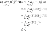
Theorem 1.Define VR as the number of falsely selected variables by robust stability selection,
We assume that the distribution of\documentclass{aastex}\usepackage{amsbsy}\usepackage{amsfonts}\usepackage{amssymb}\usepackage{bm}\usepackage{mathrsfs}\usepackage{pifont}\usepackage{stmaryrd}\usepackage{textcomp}\usepackage{portland, xspace}\usepackage{amsmath, amsxtra}\usepackage{upgreek}\pagestyle{empty}\DeclareMathSizes{10}{9}{7}{6}\begin{document}
$$\{ {{ \bf{1}}_{j \in {{ \hat S}^ \lambda }}} , j \in N \} $$
\end{document}is exchangeable for all\documentclass{aastex}\usepackage{amsbsy}\usepackage{amsfonts}\usepackage{amssymb}\usepackage{bm}\usepackage{mathrsfs}\usepackage{pifont}\usepackage{stmaryrd}\usepackage{textcomp}\usepackage{portland, xspace}\usepackage{amsmath, amsxtra}\usepackage{upgreek}\pagestyle{empty}\DeclareMathSizes{10}{9}{7}{6}\begin{document}
$$\lambda \in \Lambda$$
\end{document}and that the original procedure is not worse than random guessing (Meinshausen and Bühlmann, 2010), that is,\documentclass{aastex}\usepackage{amsbsy}\usepackage{amsfonts}\usepackage{amssymb}\usepackage{bm}\usepackage{mathrsfs}\usepackage{pifont}\usepackage{stmaryrd}\usepackage{textcomp}\usepackage{portland, xspace}\usepackage{amsmath, amsxtra}\usepackage{upgreek}\pagestyle{empty}\DeclareMathSizes{10}{9}{7}{6}\begin{document}
\begin{align*}
{ \frac { E ( \vert S \cap { { \hat S } ^ \Lambda } \vert ) } { E ( \vert N \cap { { \hat S } ^ \Lambda } \vert ) } } \ge { \frac { \vert S \vert } { \vert N \vert } } . \tag { 13 }
\end{align*}
\end{document}
For a threshold\documentclass{aastex}\usepackage{amsbsy}\usepackage{amsfonts}\usepackage{amssymb}\usepackage{bm}\usepackage{mathrsfs}\usepackage{pifont}\usepackage{stmaryrd}\usepackage{textcomp}\usepackage{portland, xspace}\usepackage{amsmath, amsxtra}\usepackage{upgreek}\pagestyle{empty}\DeclareMathSizes{10}{9}{7}{6}\begin{document}
$$ { \pi _ { { \rm { thr } } } } \in ( \frac { 1 } { 2 } , 1 )$$
\end{document}, the expected number of falsely selected variables of the proposed robust stability selection is bounded as follows:\documentclass{aastex}\usepackage{amsbsy}\usepackage{amsfonts}\usepackage{amssymb}\usepackage{bm}\usepackage{mathrsfs}\usepackage{pifont}\usepackage{stmaryrd}\usepackage{textcomp}\usepackage{portland, xspace}\usepackage{amsmath, amsxtra}\usepackage{upgreek}\pagestyle{empty}\DeclareMathSizes{10}{9}{7}{6}\begin{document}
\begin{align*}
E ( V_ \ell ^R ) \le { \frac { E ( q_ { { \Lambda ^ { - \ell } } } ^2 ) } { p \cdot ( 2 { \pi _ { { \rm { thr } } } } - 1 ) } } , \tag { 14 }
\end{align*}
\end{document}
The theorem is proved in Section 7. For all \documentclass{aastex}\usepackage{amsbsy}\usepackage{amsfonts}\usepackage{amssymb}\usepackage{bm}\usepackage{mathrsfs}\usepackage{pifont}\usepackage{stmaryrd}\usepackage{textcomp}\usepackage{portland, xspace}\usepackage{amsmath, amsxtra}\usepackage{upgreek}\pagestyle{empty}\DeclareMathSizes{10}{9}{7}{6}\begin{document}
$$\ell = 0 , 1 , .. , L$$
\end{document}, the upper bound of our method is smaller than or equal to that of ordinary stability selection, because \documentclass{aastex}\usepackage{amsbsy}\usepackage{amsfonts}\usepackage{amssymb}\usepackage{bm}\usepackage{mathrsfs}\usepackage{pifont}\usepackage{stmaryrd}\usepackage{textcomp}\usepackage{portland, xspace}\usepackage{amsmath, amsxtra}\usepackage{upgreek}\pagestyle{empty}\DeclareMathSizes{10}{9}{7}{6}\begin{document}
$${q_{{ \Lambda ^{ - \ell }}}} \le {q_ \Lambda }$$
\end{document} for all \documentclass{aastex}\usepackage{amsbsy}\usepackage{amsfonts}\usepackage{amssymb}\usepackage{bm}\usepackage{mathrsfs}\usepackage{pifont}\usepackage{stmaryrd}\usepackage{textcomp}\usepackage{portland, xspace}\usepackage{amsmath, amsxtra}\usepackage{upgreek}\pagestyle{empty}\DeclareMathSizes{10}{9}{7}{6}\begin{document}
$$\ell = 0 , 1 , .. , L$$
\end{document}. This finding implies that the proposed robust stability selection more tightly controls the error of falsely selected variables than ordinary stability selection does.
The proposed robust sample-specific stability selection method can effectively perform sample-specific analysis without causing disturbances of samples to have characteristics different from those of a target sample, because our method controls for the effect of samples using a two-stage strategy (i.e., weighted random sampling and kernel-based L1-type regularization in the sample-specific random lasso). Furthermore, the proposed method can efficiently control false positives of feature selection by using robust stability selection.
4. Monte Carlo Simulations
Monte Carlo simulations are conducted to investigate the performance of the proposed robust sample-specific stability selection method. We consider the following varying coefficient model:
\documentclass{aastex}\usepackage{amsbsy}\usepackage{amsfonts}\usepackage{amssymb}\usepackage{bm}\usepackage{mathrsfs}\usepackage{pifont}\usepackage{stmaryrd}\usepackage{textcomp}\usepackage{portland, xspace}\usepackage{amsmath, amsxtra}\usepackage{upgreek}\pagestyle{empty}\DeclareMathSizes{10}{9}{7}{6}\begin{document}
\begin{align*}
{t_i} = r_i^T \beta ( {m_ \alpha } ) + s{ \varepsilon _i} , \quad i = 1 , \ldots , n , \tag{15}
\end{align*}
\end{document}
where \documentclass{aastex}\usepackage{amsbsy}\usepackage{amsfonts}\usepackage{amssymb}\usepackage{bm}\usepackage{mathrsfs}\usepackage{pifont}\usepackage{stmaryrd}\usepackage{textcomp}\usepackage{portland, xspace}\usepackage{amsmath, amsxtra}\usepackage{upgreek}\pagestyle{empty}\DeclareMathSizes{10}{9}{7}{6}\begin{document}
$${ \varepsilon _i}$$
\end{document} are \documentclass{aastex}\usepackage{amsbsy}\usepackage{amsfonts}\usepackage{amssymb}\usepackage{bm}\usepackage{mathrsfs}\usepackage{pifont}\usepackage{stmaryrd}\usepackage{textcomp}\usepackage{portland, xspace}\usepackage{amsmath, amsxtra}\usepackage{upgreek}\pagestyle{empty}\DeclareMathSizes{10}{9}{7}{6}\begin{document}
$$N ( 0 , { \sigma ^2} )$$
\end{document} and the correlation between rl and rm is \documentclass{aastex}\usepackage{amsbsy}\usepackage{amsfonts}\usepackage{amssymb}\usepackage{bm}\usepackage{mathrsfs}\usepackage{pifont}\usepackage{stmaryrd}\usepackage{textcomp}\usepackage{portland, xspace}\usepackage{amsmath, amsxtra}\usepackage{upgreek}\pagestyle{empty}\DeclareMathSizes{10}{9}{7}{6}\begin{document}
$${ \rho ^{ \vert l - m \vert }}$$
\end{document} in a p-dimensional multivariate normal distribution with mean zero. The modulator \documentclass{aastex}\usepackage{amsbsy}\usepackage{amsfonts}\usepackage{amssymb}\usepackage{bm}\usepackage{mathrsfs}\usepackage{pifont}\usepackage{stmaryrd}\usepackage{textcomp}\usepackage{portland, xspace}\usepackage{amsmath, amsxtra}\usepackage{upgreek}\pagestyle{empty}\DeclareMathSizes{10}{9}{7}{6}\begin{document}
$$M = {m_ \alpha }$$
\end{document} is generated from a uniform distribution \documentclass{aastex}\usepackage{amsbsy}\usepackage{amsfonts}\usepackage{amssymb}\usepackage{bm}\usepackage{mathrsfs}\usepackage{pifont}\usepackage{stmaryrd}\usepackage{textcomp}\usepackage{portland, xspace}\usepackage{amsmath, amsxtra}\usepackage{upgreek}\pagestyle{empty}\DeclareMathSizes{10}{9}{7}{6}\begin{document}
$$U ( - 1 , 1 )$$
\end{document} for \documentclass{aastex}\usepackage{amsbsy}\usepackage{amsfonts}\usepackage{amssymb}\usepackage{bm}\usepackage{mathrsfs}\usepackage{pifont}\usepackage{stmaryrd}\usepackage{textcomp}\usepackage{portland, xspace}\usepackage{amsmath, amsxtra}\usepackage{upgreek}\pagestyle{empty}\DeclareMathSizes{10}{9}{7}{6}\begin{document}
$$\alpha = 1 , 2 , \ldots , n$$
\end{document}.
We consider \documentclass{aastex}\usepackage{amsbsy}\usepackage{amsfonts}\usepackage{amssymb}\usepackage{bm}\usepackage{mathrsfs}\usepackage{pifont}\usepackage{stmaryrd}\usepackage{textcomp}\usepackage{portland, xspace}\usepackage{amsmath, amsxtra}\usepackage{upgreek}\pagestyle{empty}\DeclareMathSizes{10}{9}{7}{6}\begin{document}
$$n = 600$$
\end{document} and randomly select 20% of the variables as active regulators that have nonzero coefficients for 75% of the samples (450 of the 600 samples) and zero coefficients for 25% of the samples. The remaining 80% of variables are considered as noisy features (i.e., these variables have zero coefficients for all 600 samples). The varying coefficients β for 450 samples of the active regulators are generated from \documentclass{aastex}\usepackage{amsbsy}\usepackage{amsfonts}\usepackage{amssymb}\usepackage{bm}\usepackage{mathrsfs}\usepackage{pifont}\usepackage{stmaryrd}\usepackage{textcomp}\usepackage{portland, xspace}\usepackage{amsmath, amsxtra}\usepackage{upgreek}\pagestyle{empty}\DeclareMathSizes{10}{9}{7}{6}\begin{document}
$$U ( - 5 , - 4.5 )$$
\end{document} and \documentclass{aastex}\usepackage{amsbsy}\usepackage{amsfonts}\usepackage{amssymb}\usepackage{bm}\usepackage{mathrsfs}\usepackage{pifont}\usepackage{stmaryrd}\usepackage{textcomp}\usepackage{portland, xspace}\usepackage{amsmath, amsxtra}\usepackage{upgreek}\pagestyle{empty}\DeclareMathSizes{10}{9}{7}{6}\begin{document}
$$U ( 4.5 , 5 )$$
\end{document} in descending (half of active regulators) and ascending (the other half) order, as shown in Figure 1.
Coefficient functions with a modulator.
We consider \documentclass{aastex}\usepackage{amsbsy}\usepackage{amsfonts}\usepackage{amssymb}\usepackage{bm}\usepackage{mathrsfs}\usepackage{pifont}\usepackage{stmaryrd}\usepackage{textcomp}\usepackage{portland, xspace}\usepackage{amsmath, amsxtra}\usepackage{upgreek}\pagestyle{empty}\DeclareMathSizes{10}{9}{7}{6}\begin{document}
$$p = 50 , 600 , 1000 , 2000$$
\end{document}, \documentclass{aastex}\usepackage{amsbsy}\usepackage{amsfonts}\usepackage{amssymb}\usepackage{bm}\usepackage{mathrsfs}\usepackage{pifont}\usepackage{stmaryrd}\usepackage{textcomp}\usepackage{portland, xspace}\usepackage{amsmath, amsxtra}\usepackage{upgreek}\pagestyle{empty}\DeclareMathSizes{10}{9}{7}{6}\begin{document}
$$s = 1 , 3 , 5$$
\end{document} for Example 1 (\documentclass{aastex}\usepackage{amsbsy}\usepackage{amsfonts}\usepackage{amssymb}\usepackage{bm}\usepackage{mathrsfs}\usepackage{pifont}\usepackage{stmaryrd}\usepackage{textcomp}\usepackage{portland, xspace}\usepackage{amsmath, amsxtra}\usepackage{upgreek}\pagestyle{empty}\DeclareMathSizes{10}{9}{7}{6}\begin{document}
$$\rho = 0.5$$
\end{document}), Example 2 (\documentclass{aastex}\usepackage{amsbsy}\usepackage{amsfonts}\usepackage{amssymb}\usepackage{bm}\usepackage{mathrsfs}\usepackage{pifont}\usepackage{stmaryrd}\usepackage{textcomp}\usepackage{portland, xspace}\usepackage{amsmath, amsxtra}\usepackage{upgreek}\pagestyle{empty}\DeclareMathSizes{10}{9}{7}{6}\begin{document}
$$\rho = 0.7$$
\end{document}), and Example 3 (\documentclass{aastex}\usepackage{amsbsy}\usepackage{amsfonts}\usepackage{amssymb}\usepackage{bm}\usepackage{mathrsfs}\usepackage{pifont}\usepackage{stmaryrd}\usepackage{textcomp}\usepackage{portland, xspace}\usepackage{amsmath, amsxtra}\usepackage{upgreek}\pagestyle{empty}\DeclareMathSizes{10}{9}{7}{6}\begin{document}
$$\rho = 0.9$$
\end{document}). We then perform sample-specific regression modeling for five randomly selected target samples based on the varying coefficient model. In the sample-specific random lasso, we consider \documentclass{aastex}\usepackage{amsbsy}\usepackage{amsfonts}\usepackage{amssymb}\usepackage{bm}\usepackage{mathrsfs}\usepackage{pifont}\usepackage{stmaryrd}\usepackage{textcomp}\usepackage{portland, xspace}\usepackage{amsmath, amsxtra}\usepackage{upgreek}\pagestyle{empty}\DeclareMathSizes{10}{9}{7}{6}\begin{document}
$$B = 100$$
\end{document} random subsets and \documentclass{aastex}\usepackage{amsbsy}\usepackage{amsfonts}\usepackage{amssymb}\usepackage{bm}\usepackage{mathrsfs}\usepackage{pifont}\usepackage{stmaryrd}\usepackage{textcomp}\usepackage{portland, xspace}\usepackage{amsmath, amsxtra}\usepackage{upgreek}\pagestyle{empty}\DeclareMathSizes{10}{9}{7}{6}\begin{document}
$$v = 0.9$$
\end{document} for weighted random sampling. The tuning parameter l of the robust stability selection method that minimizes estimation error is selected.
We evaluate our method based on the accuracy of feature selection given as the average of the true positive rate (i.e., the average number of the truly nonzero coefficients that are correctly estimated as nonzero, which we denote as TP) and the true negative rate (i.e., the average percentage of the truly zero coefficients that are correctly estimated as zero, which we denote as TN).
The results of our method (R.SS.STB) are compared with results of the ELA, which is not a sample-specific approach; NP; and sample-specific stability selection based on the maximum value of the selection probability (O.SS.STB). The simulation is repeated 100 times for Examples 1, 2, and 3.
Table 1 gives the feature selection accuracy (i.e., the average of TP and TN). The stability selection approaches (i.e., O.SS.STB and R.SS.STB) show outstanding performance for high-dimensional data analysis. In particular, the proposed robust sample-specific stability selection method shows effectiveness compared with the existing methods. Furthermore, the outstanding performance of our method can also be seen in the large variance of the residual term (i.e., \documentclass{aastex}\usepackage{amsbsy}\usepackage{amsfonts}\usepackage{amssymb}\usepackage{bm}\usepackage{mathrsfs}\usepackage{pifont}\usepackage{stmaryrd}\usepackage{textcomp}\usepackage{portland, xspace}\usepackage{amsmath, amsxtra}\usepackage{upgreek}\pagestyle{empty}\DeclareMathSizes{10}{9}{7}{6}\begin{document}
$$s = 3 , 5$$
\end{document}). The ELA shows poor results for all simulation settings because the method cannot control the effect of samples on sample-specific analysis.
Denotes significant differences in performance between other methods at significant level \documentclass{aastex}\usepackage{amsbsy}\usepackage{amsfonts}\usepackage{amssymb}\usepackage{bm}\usepackage{mathrsfs}\usepackage{pifont}\usepackage{stmaryrd}\usepackage{textcomp}\usepackage{portland, xspace}\usepackage{amsmath, amsxtra}\usepackage{upgreek}\pagestyle{empty}\DeclareMathSizes{10}{9}{7}{6}\begin{document}
$$\alpha = 0.05$$
\end{document}.
ELAs, elastic nets; NP, NetworkProfiler.
Boldface indicates the best performance among the methods (i.e., O.SS.STB, R.SS.STB, NP, and ELA).
We also show the estimation accuracy given as the following mean squared error (MSE):
\documentclass{aastex}\usepackage{amsbsy}\usepackage{amsfonts}\usepackage{amssymb}\usepackage{bm}\usepackage{mathrsfs}\usepackage{pifont}\usepackage{stmaryrd}\usepackage{textcomp}\usepackage{portland, xspace}\usepackage{amsmath, amsxtra}\usepackage{upgreek}\pagestyle{empty}\DeclareMathSizes{10}{9}{7}{6}\begin{document}
\begin{align*}
{ \rm { MSE } } = \frac { 1 } { 5 } \sum \limits_ { i = 1 } ^5 { ( { t_i } - r_i^T \hat \beta ( { m_i } ) ) ^2 } . \tag { 16 }
\end{align*}
\end{document}
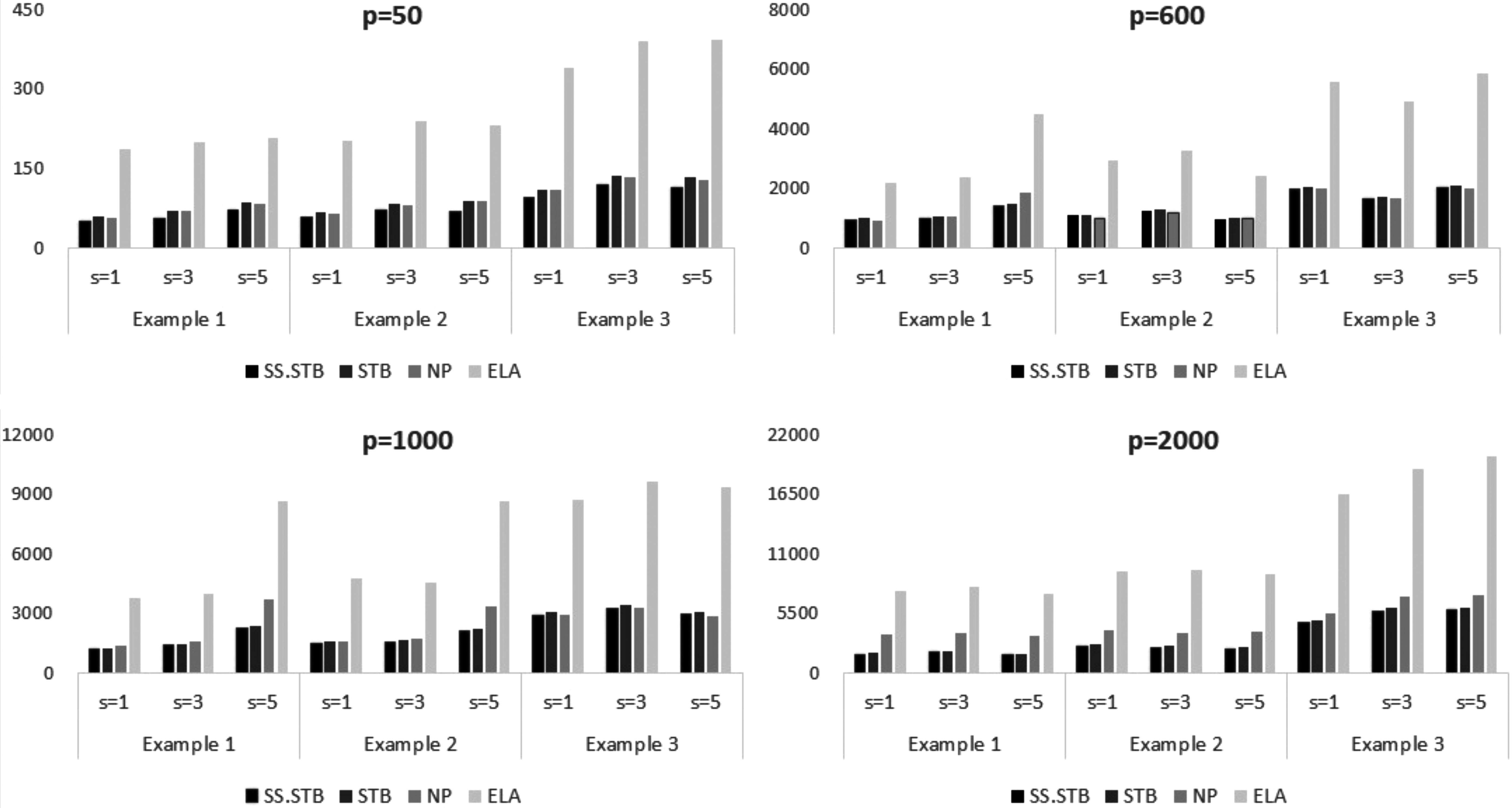
Figure 2 shows the average of the MSE of 100 simulated data sets. The red lines indicate the best performance among the four methods (i.e., R.SS.STB, O.SS.STB, NP, and ELA). As shown in Figure 2, our method (R.SS.STB) shows outstanding performance for estimation accuracy. Although our proposed method does not show competitive results for \documentclass{aastex}\usepackage{amsbsy}\usepackage{amsfonts}\usepackage{amssymb}\usepackage{bm}\usepackage{mathrsfs}\usepackage{pifont}\usepackage{stmaryrd}\usepackage{textcomp}\usepackage{portland, xspace}\usepackage{amsmath, amsxtra}\usepackage{upgreek}\pagestyle{empty}\DeclareMathSizes{10}{9}{7}{6}\begin{document}
$$p = 600$$
\end{document}, our method does show effective results overall. It can also be seen that the methods based on the stability selection framework (i.e., O.SS.STB and R.SS.STB) show efficient results, like good feature selection accuracy, for high-dimensional data analysis (i.e., \documentclass{aastex}\usepackage{amsbsy}\usepackage{amsfonts}\usepackage{amssymb}\usepackage{bm}\usepackage{mathrsfs}\usepackage{pifont}\usepackage{stmaryrd}\usepackage{textcomp}\usepackage{portland, xspace}\usepackage{amsmath, amsxtra}\usepackage{upgreek}\pagestyle{empty}\DeclareMathSizes{10}{9}{7}{6}\begin{document}
$$p = 1000 , 2000$$
\end{document}). We expect that the proposed robust sample-specific stability selection method can be a useful tool for high-dimensional varying coefficient modeling.
Mean squared error in simulation studies.
5. Real Data Analysis: Sanger Genomics of Drug Sensitivity in Cancer Data Set
We apply the proposed method to the Sanger Genomics of Drug Sensitivity in Cancer data set from the Cancer Genome Project, which is publicly available (www.cancerrxgene.org/). The data set consists of the gene expression levels of 13,331 genes and the copy numbers, mutation statuses, and IC50 values of 140 drugs (i.e., half maximal inhibitory drug concentrations, which indicate the drug sensitivity of cell lines) for 654 cell lines.
To construct anticancer drug sensitivity-specific gene network, we use the adaptive NP (Park et al., 2017) in the sample-specific random lasso.
We construct anticancer drug sensitivity-specific gene networks based on the varying coefficient model in Equation (2). In other words, we perform sample-specific analysis according to the anticancer drug response given as the IC50 value of a drug. To construct drug response-specific gene networks, we consider 99 drugs that have nonmissing IC50 values for >600 cell lines and the 10 target genes that have the highest coefficient of variation of expression levels. For each target gene, we extract the 10 drugs that have the highest absolute correlations between the IC50 value of the drug and the expression level of the target gene. We then perform varying coefficient modeling based on the expression levels of 1111 genes, which were considered as candidate regulators in Park et al. (2017). For each target gene, we construct 100 gene networks (10 drugs\documentclass{aastex}\usepackage{amsbsy}\usepackage{amsfonts}\usepackage{amssymb}\usepackage{bm}\usepackage{mathrsfs}\usepackage{pifont}\usepackage{stmaryrd}\usepackage{textcomp}\usepackage{portland, xspace}\usepackage{amsmath, amsxtra}\usepackage{upgreek}\pagestyle{empty}\DeclareMathSizes{10}{9}{7}{6}\begin{document}
$$\times$$
\end{document}the IC50 values of 10 cell lines). In short, we construct 1000 gene networks based on 10 target genes with 10 anticancer drugs in each of the 10 cell lines (i.e., the 5 cell lines with the highest and lowest IC50 values are selected as the target samples for drug-resistant and drug-sensitive gene networks, respectively). In the sample-specific random lasso, we consider \documentclass{aastex}\usepackage{amsbsy}\usepackage{amsfonts}\usepackage{amssymb}\usepackage{bm}\usepackage{mathrsfs}\usepackage{pifont}\usepackage{stmaryrd}\usepackage{textcomp}\usepackage{portland, xspace}\usepackage{amsmath, amsxtra}\usepackage{upgreek}\pagestyle{empty}\DeclareMathSizes{10}{9}{7}{6}\begin{document}
$$B = 100$$
\end{document} and \documentclass{aastex}\usepackage{amsbsy}\usepackage{amsfonts}\usepackage{amssymb}\usepackage{bm}\usepackage{mathrsfs}\usepackage{pifont}\usepackage{stmaryrd}\usepackage{textcomp}\usepackage{portland, xspace}\usepackage{amsmath, amsxtra}\usepackage{upgreek}\pagestyle{empty}\DeclareMathSizes{10}{9}{7}{6}\begin{document}
$$v = 0.9$$
\end{document} for weighted random sampling, and the tuning parameter ℓ that minimizes the estimation error is selected.
A summary of the constructed 1000 gene networks using our method is given in Table 2. Table 2 shows the average numbers of selected genes in the models for drug-resistant (R), drug-sensitive (S), and total (T) samples. It can be seen that the ordinary stability selection (O.SS.STB) tends to select a large number of genes compared with other methods. The result may be caused by the use of the lambda maximizing the selection probability of variables in O.SS.STB. We also show the p-value of the t-test for comparing the number of selected genes in drug-sensitive and drug-resistant samples. As shown in Table 2, sample-specific analysis approaches (i.e., R.SS.STB, O.SS.STB, and NP) show different modeling results in drug-sensitive and drug-resistant samples, whereas the ELA cannot show the significantly different results.
Summary of the Constructed Gene Network
R.SS.STB
O.SS.STB
NP
ELA
No. of genes
T
66.2
274.6
84.6
77.2
R
103.4
310.6
95.4
80.4
S
29.0
238.6
73.9
74.1
p
0.0000
0.0002
0.0376
0.5309
To evaluate the proposed robust sample-specific stability selection method (R.SS.STB), we compare the median absolute error (MAE) of our method with those of the ELA, NP, and stability selection (O.SS.STB) methods. Figure 3 shows the boxplots of the MAEs of 10 anticancer drugs for 10 target genes, where the numbers on the boxes indicate the mean of MAEs for the 10 drugs, where the numbers in parentheses are the corresponding standard deviations. As shown in Figure 3, the stability selection framework (R.SS.STB and O.SS.STB) shows an outstanding estimation accuracy performance, as in the simulation studies. In particular, the proposed robust sample-specific stability selection method exhibits effective performance in modeling for target genes as compared with the existing methods.
Boxplot of estimation error (MAE). MAE, median absolute error.
For anticancer drug-resistant and drug-sensitive samples, we visualize the constructed gene regulatory networks of 10 target genes with their highly correlated 10 drugs. For selected regulators in the varying coefficient model for a target sample with a drug, we compute the variances of the estimated varying coefficients of the 10 target samples corresponding to the 10 IC50 values of the drug (i.e., \documentclass{aastex}\usepackage{amsbsy}\usepackage{amsfonts}\usepackage{amssymb}\usepackage{bm}\usepackage{mathrsfs}\usepackage{pifont}\usepackage{stmaryrd}\usepackage{textcomp}\usepackage{portland, xspace}\usepackage{amsmath, amsxtra}\usepackage{upgreek}\pagestyle{empty}\DeclareMathSizes{10}{9}{7}{6}\begin{document}
$${ \rm{Var}} ( \hat \beta ( {m_ \alpha } ) )$$
\end{document} for \documentclass{aastex}\usepackage{amsbsy}\usepackage{amsfonts}\usepackage{amssymb}\usepackage{bm}\usepackage{mathrsfs}\usepackage{pifont}\usepackage{stmaryrd}\usepackage{textcomp}\usepackage{portland, xspace}\usepackage{amsmath, amsxtra}\usepackage{upgreek}\pagestyle{empty}\DeclareMathSizes{10}{9}{7}{6}\begin{document}
$$\alpha = 1 , .. , 10$$
\end{document}).
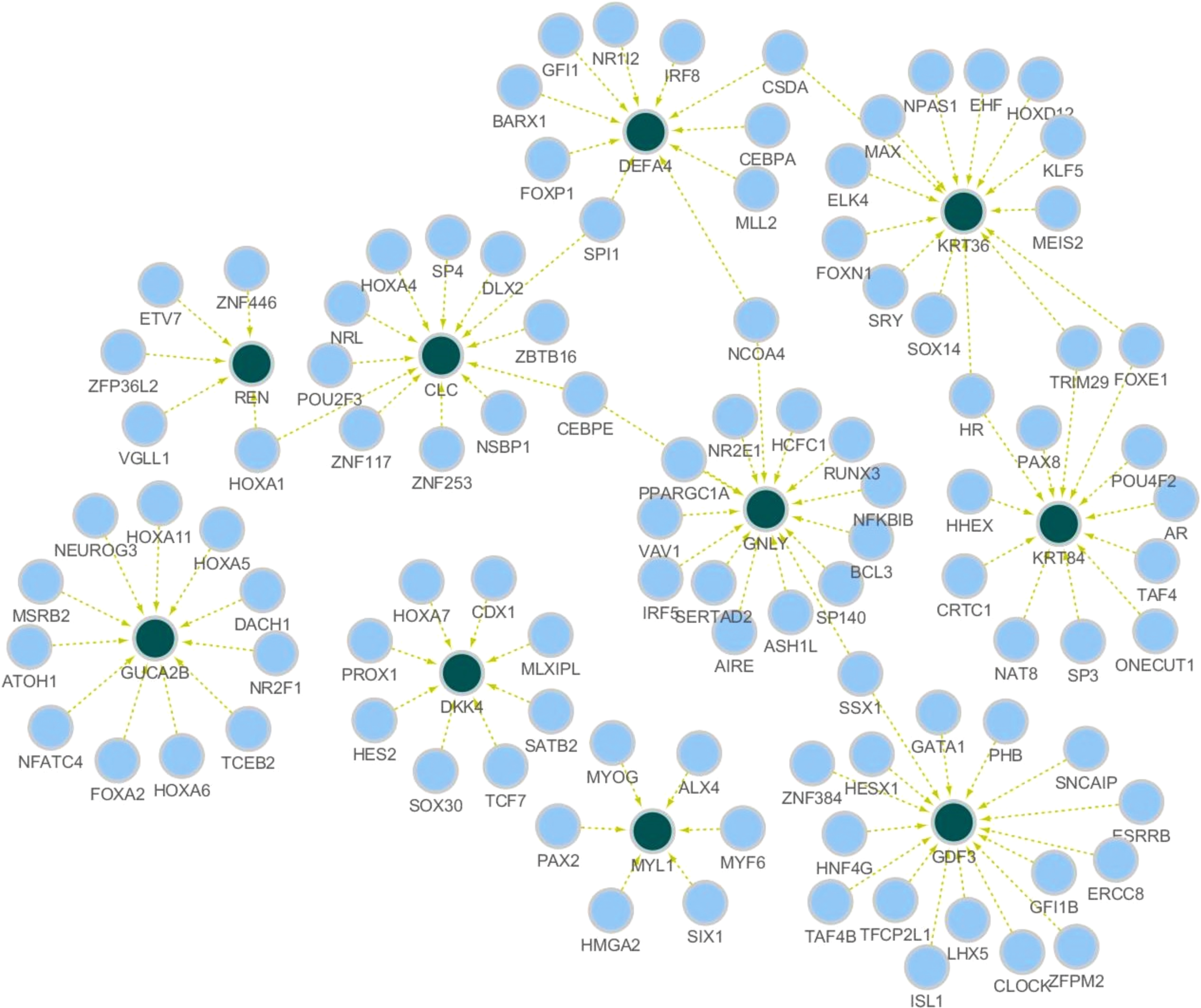
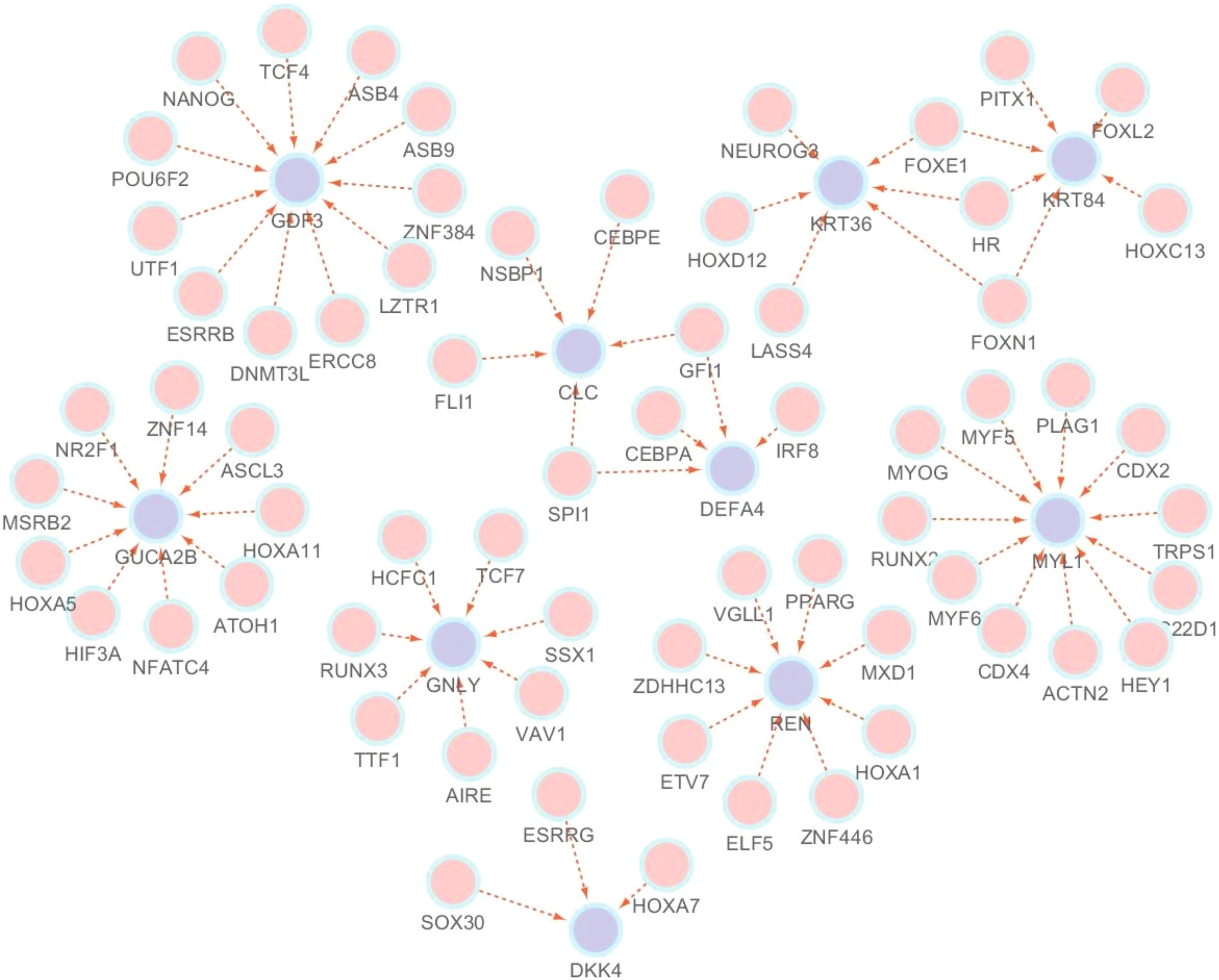
We extract the three regulators that have the largest variance of the coefficients from each model. We then visualize the constructed gene networks based on the extracted three genes for the most drug-sensitive sample (i.e., for the smallest IC50 value of a drug) and the most drug-resistant sample (i.e., for the largest IC50 value of a drug) in Figures 4 and 5, respectively.
Gene regulatory network for the anticancer drug-resistant sample.
Gene regulatory network for the anticancer drug-sensitive sample.
As shown in Figures 4 and 5, the gene-to-gene regulatory relationships have different patterns for drug-sensitive and drug-resistant cell lines. For instance, the genes SPI1, FLI1, NSBP1, CEBPE, and GDI1 are selected as active regulators for the target gene CLC in the drug-sensitive sample (Fig. 5), whereas only NSBP1 and CEBPE are selected in the models for the resistant samples (Fig. 4). From these results, we can see that each patient (cell line) corresponding to a specific anticancer drug response has different molecular mechanisms for cancer. This finding implies that identifying individual features related to cancer is a crucial issue in anticancer therapy.
We also perform crucial regulator identification in the constructed anticancer drug sensitivity-specific gene regulatory networks as shown in Figures 4 and 5. The genes selected for more than two target genes are considered as crucial regulators. Table 3 shows the selected regulators and related diseases, where the columns “S” and “R” indicate the selection frequency of the regulator in the visualized gene networks for the drug-sensitive and drug-resistant samples, respectively. We can see from Table 3 strong pieces of evidence that the regulators selected by our approach are cancer-related genes. This result implies that the proposed robust sample-specific stability selection method provides biologically reliable results for gene selection in gene network construction.
Crucial Regulators in the Drug Response-Specific Gene Networks
Regulators
S
R
Diseases
Evidence
CEBPE
2
Acute myelogenous leukemia
Pabst et al. (2001); Pabst and Mueller (2009); Sun et al., (2015)
Nonsmall cell lung cancer, lung cancer, prostate cancers, bladder cancer cells, etc.
Zhou et al. (2012); Tan et al. (2016); Hatakeyama (2012)
In short, our method can be a useful tool for sample-specific gene regulatory network construction.
6. Concluding Remarks
We have introduced a novel method for sample-specific analysis, called robust sample-specific stability selection. We have first focused on demonstrating that ordinary stability selection provides feature selection results that are sensitive to the regularization parameter, and we then propose robust stability selection. We have shown that the proposed robust stability selection method has attractive theoretical properties as a feature selection tool. For the iterative modeling procedure in stability selection, we have also proposed a sample-specific random lasso based on weighted random sampling and kernel-based L1-type regularization to effectively perform sample-specific analysis.
We can see from numerical studies that the proposed robust sample-specific stability selection method performs sample-specific analysis effectively from the viewpoints of estimation and feature selection accuracy. Furthermore, our method also provides biologically reliable results for gene selection in gene network construction.
We selected the stability selection threshold \documentclass{aastex}\usepackage{amsbsy}\usepackage{amsfonts}\usepackage{amssymb}\usepackage{bm}\usepackage{mathrsfs}\usepackage{pifont}\usepackage{stmaryrd}\usepackage{textcomp}\usepackage{portland, xspace}\usepackage{amsmath, amsxtra}\usepackage{upgreek}\pagestyle{empty}\DeclareMathSizes{10}{9}{7}{6}\begin{document}
$${ \pi _{{ \rm{thr}}}}$$
\end{document} based on the estimation error of the varying coefficient model. However, choosing the threshold \documentclass{aastex}\usepackage{amsbsy}\usepackage{amsfonts}\usepackage{amssymb}\usepackage{bm}\usepackage{mathrsfs}\usepackage{pifont}\usepackage{stmaryrd}\usepackage{textcomp}\usepackage{portland, xspace}\usepackage{amsmath, amsxtra}\usepackage{upgreek}\pagestyle{empty}\DeclareMathSizes{10}{9}{7}{6}\begin{document}
$${ \pi _{{ \rm{thr}}}}$$
\end{document} is a crucial issue because feature selection results heavily rely on the threshold in the stability selection procedure. We consider information criteria for choosing the threshold as future work for this line of research. In addition, in this study, we focus on false positives of feature selection. However, controlling false negatives is also a vital matter in feature selection. Further work remains to be done toward developing a sample-specific analysis strategy that can effectively control false positives and false negatives simultaneously.
7. Appendix: Proof of Theorem 1
We prove the theoretical property of our method given in Theorem 1 in line with Top-k stability selection (Zhou et al., 2013).
Let Ii for \documentclass{aastex}\usepackage{amsbsy}\usepackage{amsfonts}\usepackage{amssymb}\usepackage{bm}\usepackage{mathrsfs}\usepackage{pifont}\usepackage{stmaryrd}\usepackage{textcomp}\usepackage{portland, xspace}\usepackage{amsmath, amsxtra}\usepackage{upgreek}\pagestyle{empty}\DeclareMathSizes{10}{9}{7}{6}\begin{document}
$$i = 1 , 2$$
\end{document} be two random subsets of T with size \documentclass{aastex}\usepackage{amsbsy}\usepackage{amsfonts}\usepackage{amssymb}\usepackage{bm}\usepackage{mathrsfs}\usepackage{pifont}\usepackage{stmaryrd}\usepackage{textcomp}\usepackage{portland, xspace}\usepackage{amsmath, amsxtra}\usepackage{upgreek}\pagestyle{empty}\DeclareMathSizes{10}{9}{7}{6}\begin{document}
$$\left\lfloor {n / 2} \right\rfloor$$
\end{document} and \documentclass{aastex}\usepackage{amsbsy}\usepackage{amsfonts}\usepackage{amssymb}\usepackage{bm}\usepackage{mathrsfs}\usepackage{pifont}\usepackage{stmaryrd}\usepackage{textcomp}\usepackage{portland, xspace}\usepackage{amsmath, amsxtra}\usepackage{upgreek}\pagestyle{empty}\DeclareMathSizes{10}{9}{7}{6}\begin{document}
$${{\bf I}_1} \cap {{\bf I}_2} = \emptyset$$
\end{document}. For the sample-specific random lasso, we let \documentclass{aastex}\usepackage{amsbsy}\usepackage{amsfonts}\usepackage{amssymb}\usepackage{bm}\usepackage{mathrsfs}\usepackage{pifont}\usepackage{stmaryrd}\usepackage{textcomp}\usepackage{portland, xspace}\usepackage{amsmath, amsxtra}\usepackage{upgreek}\pagestyle{empty}\DeclareMathSizes{10}{9}{7}{6}\begin{document}
$${\bf I}_1^ \alpha$$
\end{document} and \documentclass{aastex}\usepackage{amsbsy}\usepackage{amsfonts}\usepackage{amssymb}\usepackage{bm}\usepackage{mathrsfs}\usepackage{pifont}\usepackage{stmaryrd}\usepackage{textcomp}\usepackage{portland, xspace}\usepackage{amsmath, amsxtra}\usepackage{upgreek}\pagestyle{empty}\DeclareMathSizes{10}{9}{7}{6}\begin{document}
$${\bf I}_2^ \alpha$$
\end{document} be weighted random subsets for modeling the \documentclass{aastex}\usepackage{amsbsy}\usepackage{amsfonts}\usepackage{amssymb}\usepackage{bm}\usepackage{mathrsfs}\usepackage{pifont}\usepackage{stmaryrd}\usepackage{textcomp}\usepackage{portland, xspace}\usepackage{amsmath, amsxtra}\usepackage{upgreek}\pagestyle{empty}\DeclareMathSizes{10}{9}{7}{6}\begin{document}
$$\alpha th$$
\end{document} target sample with size \documentclass{aastex}\usepackage{amsbsy}\usepackage{amsfonts}\usepackage{amssymb}\usepackage{bm}\usepackage{mathrsfs}\usepackage{pifont}\usepackage{stmaryrd}\usepackage{textcomp}\usepackage{portland, xspace}\usepackage{amsmath, amsxtra}\usepackage{upgreek}\pagestyle{empty}\DeclareMathSizes{10}{9}{7}{6}\begin{document}
$$\left\lfloor {n / 2} \right\rfloor \times v$$
\end{document}, where \documentclass{aastex}\usepackage{amsbsy}\usepackage{amsfonts}\usepackage{amssymb}\usepackage{bm}\usepackage{mathrsfs}\usepackage{pifont}\usepackage{stmaryrd}\usepackage{textcomp}\usepackage{portland, xspace}\usepackage{amsmath, amsxtra}\usepackage{upgreek}\pagestyle{empty}\DeclareMathSizes{10}{9}{7}{6}\begin{document}
$$0 < v < 1$$
\end{document}. Because the sample-specific random lasso performs feature selection based on the weighted random subset \documentclass{aastex}\usepackage{amsbsy}\usepackage{amsfonts}\usepackage{amssymb}\usepackage{bm}\usepackage{mathrsfs}\usepackage{pifont}\usepackage{stmaryrd}\usepackage{textcomp}\usepackage{portland, xspace}\usepackage{amsmath, amsxtra}\usepackage{upgreek}\pagestyle{empty}\DeclareMathSizes{10}{9}{7}{6}\begin{document}
$${\bf{I}}_1^ \alpha$$
\end{document} and \documentclass{aastex}\usepackage{amsbsy}\usepackage{amsfonts}\usepackage{amssymb}\usepackage{bm}\usepackage{mathrsfs}\usepackage{pifont}\usepackage{stmaryrd}\usepackage{textcomp}\usepackage{portland, xspace}\usepackage{amsmath, amsxtra}\usepackage{upgreek}\pagestyle{empty}\DeclareMathSizes{10}{9}{7}{6}\begin{document}
$${\bf {I}}_2^ \alpha$$
\end{document}, we define the simultaneous selected set for sample-specific random lasso as follows,
\documentclass{aastex}\usepackage{amsbsy}\usepackage{amsfonts}\usepackage{amssymb}\usepackage{bm}\usepackage{mathrsfs}\usepackage{pifont}\usepackage{stmaryrd}\usepackage{textcomp}\usepackage{portland, xspace}\usepackage{amsmath, amsxtra}\usepackage{upgreek}\pagestyle{empty}\DeclareMathSizes{10}{9}{7}{6}\begin{document}
\begin{align*}
{ \hat S^{smt , \lambda }} = { \hat S^ \lambda } ( { \bf{I}}_1^ \alpha ) \cap { \hat S^ \lambda } ( { \bf{I}}_2^ \alpha ) . \tag{17}
\end{align*}
\end{document}
The corresponding simultaneous selection probability for any set \documentclass{aastex}\usepackage{amsbsy}\usepackage{amsfonts}\usepackage{amssymb}\usepackage{bm}\usepackage{mathrsfs}\usepackage{pifont}\usepackage{stmaryrd}\usepackage{textcomp}\usepackage{portland, xspace}\usepackage{amsmath, amsxtra}\usepackage{upgreek}\pagestyle{empty}\DeclareMathSizes{10}{9}{7}{6}\begin{document}
$${J_ \alpha } \subseteq \{ 1 , \ldots p \} $$
\end{document} is defined as
\documentclass{aastex}\usepackage{amsbsy}\usepackage{amsfonts}\usepackage{amssymb}\usepackage{bm}\usepackage{mathrsfs}\usepackage{pifont}\usepackage{stmaryrd}\usepackage{textcomp}\usepackage{portland, xspace}\usepackage{amsmath, amsxtra}\usepackage{upgreek}\pagestyle{empty}\DeclareMathSizes{10}{9}{7}{6}\begin{document}
\begin{align*}
\hat \Pi _{{J_ \alpha }}^{smt , \lambda } = {P^*} ( {J_ \alpha } \subseteq { \hat S^{smt , \lambda }} ) , \tag{18}
\end{align*}
\end{document}
where \documentclass{aastex}\usepackage{amsbsy}\usepackage{amsfonts}\usepackage{amssymb}\usepackage{bm}\usepackage{mathrsfs}\usepackage{pifont}\usepackage{stmaryrd}\usepackage{textcomp}\usepackage{portland, xspace}\usepackage{amsmath, amsxtra}\usepackage{upgreek}\pagestyle{empty}\DeclareMathSizes{10}{9}{7}{6}\begin{document}
$${P^*}$$
\end{document} is with respect to the random splitting and any additional randomness of the sample-specific random lasso.
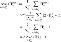
Lemma 1.For any set\documentclass{aastex}\usepackage{amsbsy}\usepackage{amsfonts}\usepackage{amssymb}\usepackage{bm}\usepackage{mathrsfs}\usepackage{pifont}\usepackage{stmaryrd}\usepackage{textcomp}\usepackage{portland, xspace}\usepackage{amsmath, amsxtra}\usepackage{upgreek}\pagestyle{empty}\DeclareMathSizes{10}{9}{7}{6}\begin{document}
$${J_ \alpha } \subseteq \{ 1 , \ldots p \} $$
\end{document}, a lower bound for the simultaneous selection probability of the robust stability selection is given as
where \documentclass{aastex}\usepackage{amsbsy}\usepackage{amsfonts}\usepackage{amssymb}\usepackage{bm}\usepackage{mathrsfs}\usepackage{pifont}\usepackage{stmaryrd}\usepackage{textcomp}\usepackage{portland, xspace}\usepackage{amsmath, amsxtra}\usepackage{upgreek}\pagestyle{empty}\DeclareMathSizes{10}{9}{7}{6}\begin{document}
$$\vert N \vert$$
\end{document} is a number of variables in the set \documentclass{aastex}\usepackage{amsbsy}\usepackage{amsfonts}\usepackage{amssymb}\usepackage{bm}\usepackage{mathrsfs}\usepackage{pifont}\usepackage{stmaryrd}\usepackage{textcomp}\usepackage{portland, xspace}\usepackage{amsmath, amsxtra}\usepackage{upgreek}\pagestyle{empty}\DeclareMathSizes{10}{9}{7}{6}\begin{document}
$$N = \{ \, j:{ \beta _j} = 0 \} $$
\end{document}, \documentclass{aastex}\usepackage{amsbsy}\usepackage{amsfonts}\usepackage{amssymb}\usepackage{bm}\usepackage{mathrsfs}\usepackage{pifont}\usepackage{stmaryrd}\usepackage{textcomp}\usepackage{portland, xspace}\usepackage{amsmath, amsxtra}\usepackage{upgreek}\pagestyle{empty}\DeclareMathSizes{10}{9}{7}{6}\begin{document}
$$E { ( { q_ { { \Lambda ^ { - \ell } } } } ) ^2 } = { E_ { j \in N } } ( q_ { \Lambda _j^ { - \ell } } ^2 ) = \frac { 1 } { { \vert N \vert } } \sum \nolimits_ { j \in N } q_ { \Lambda _j^ { - \ell } } ^2$$
\end{document}, and (b) holds based on \documentclass{aastex}\usepackage{amsbsy}\usepackage{amsfonts}\usepackage{amssymb}\usepackage{bm}\usepackage{mathrsfs}\usepackage{pifont}\usepackage{stmaryrd}\usepackage{textcomp}\usepackage{portland, xspace}\usepackage{amsmath, amsxtra}\usepackage{upgreek}\pagestyle{empty}\DeclareMathSizes{10}{9}{7}{6}\begin{document}
$$\vert N \vert < p$$
\end{document}.
Footnotes
Acknowledgments
This research was supported by MEXT as Priority Issue on Post-K Computer (hp 150265, hp 160219, hp 170227, hp 180198) and Innovation Area 15H05912). M.Y. is supported by the JST PRESTO program JPMJPR165A and partly supported by MEXT KAKENHI 16H06299.
Author Disclosure Statement
The authors declare that there are no competing financial interests.
References
1.
ChariotA., and CastronovoV.1996. Detection of HOXA1 expression in human breast cancer. Biochem. Biophys. Res. Commun. 222, 292–297.
2.
DamiolaF., ByrnesG., MoissonnierM., et al.2013. Contribution of ATM and FOXE1 (TTF2) to risk of papillary thyroid carcinoma in Belarusian children exposed to radiation. Int. J. Cancer, 134, 1659–1668.
3.
HatakeyamaS.2012. Early evidence for the role of TRIM29 in multiple cancer models. Expert. Opin. Ther. Targets, 20, 767–770.
4.
JiangP., FreedmanM.L., LiuJ.S., et al.2015. Inference of transcriptional regulation in cancers. Proc. Natl Acad. Sci. U. S. A. 112, 7731–7736.
5.
KazanjianA., GrossE.A., and GrimesH.L.2014. The growth factor independence-1 transcription factor: New functions and new insights. Crit. Rev. Oncol. Hematol. 59, 85–97.
6.
KollaraA., and BrownT.J.2012. Expression and function of nuclear receptor co-activator 4: Evidence of a potential role independent of co-activator activity. Cell. Mol. Life. Sci. 69, 3895–3909.
7.
LandaI., Ruiz-LlorenteS., Montero-CondeC., et al.2009. The variant rs1867277 in FOXE1 gene confers thyroid cancer susceptibility through the recruitment of USF1/USF2 transcription factors. PLoS Genet. 5, e1000637.
8.
LouH., LiH., YeagerM., et al.2012. Promoter variants in the MSMB gene associated with prostate cancer regulate MSMB/NCOA4 fusion transcripts. Hum. Genet. 131, 1453–1466.
9.
MatsumotoG., YajimaN., SaitoH., et al.2010. Cold shock domain protein A (CSDA) overexpression inhibits tumor growth and lymph node metastasis in a mouse model of squamous cell carcinoma. Clin. Exp. Metastasis, 27, 539–547.
10.
MazarJ., and PereraR.J.2012. Identification and characterization of a human prostate cancer specific long non-coding RNA. Int. J. Biosci. Biochem. Bioinforma. 3.
11.
MeinshausenN., and BühlmannP.2010. Stability selection. J. R. Stat. Soc. Ser. B, 72, 417–473.
12.
MondM., BullockM., YaoY., et al.2015. Somatic Mutations of FOXE1 in papillary thyroid cancer. Thyroid, 25, 904–910.
13.
PabstT., and MuellerB.U.2009. Complexity of CEBPA dysregulation in human acute myeloid leukemia. Clin. Cancer. Res. 15, 5303–5307.
14.
PabstT., MuellerB.U., HarakawaN., et al.2001. AML1-ETO downregulates the granulocytic differentiation factor C/EBPalpha in t(8;21) myeloid leukemia. Nat. Med. 7, 444–451.
15.
ParkH., ImotoS., and MiyanoS.2015. Recursive random lasso (RRLasso) for identifying anti-cancer drug targets. PLoS One, 10, e0141869.
16.
ParkH., ShimamuraT., ImotoS., et al., 2017. Adaptive NetworkProfiler for identifying cancer characteristic-specific gene regulatory networks. J. Comput. Biol. 25, 130–145.
17.
ShimamuraT., ImotoS., ShimadaY., et al.2011. A novel network profiling analysis reveals system changes in epithelial-mesenchymal transition. PLoS One, 6, e20804.
18.
SunJ., ZhengJ., TangL., et al.2015. Association between CEBPE variant and childhood acute leukemia risk: Eevidence from a neta-analysis of 22 studies. PLoS One, 10, e0125657.
19.
TanS.T., LiuS.Y., and WuB.2016. TRIM29 overexpression promotes proliferation and survival of bladder cancer cells through NF-kB Signaling. Cancer Res. Treat. 48, 1302–1312.
20.
TibshiraniR.1996. Regression shrinkage and selection via the lasso. J. R. Stat. Soc. Ser. B, 73, 273–282.
21.
WangS., NanB., RossetetS., et al.2011. Random lasso. Ann. Appl. Stat. 5, 468–485.
22.
Wardwell-OzgoJ., DogrulukT., GiffordA., et al.2014. HOXA1 drives melanoma tumor growth and metastasis and elicits an invasion gene expression signature that prognosticates clinical outcome. Oncogene, 33, 1017–1026.
23.
WatanabeY., MaedaI., OikawaR., et al.2013. Aberrant DNA methylation status of DNA repair genes in breast cancer treated with neoadjuvant chemotherapy. Genes Cells, 18, 1120–1130.
24.
XiaoF., BaiY., ChenZ., et al., 2014. Downregulation of HOXA1 gene affects small cell lung cancer cell survival and chemoresistance under the regulation of miR-100. Eur. J. Cancer, 50, 1541–1554.
25.
YiB., WangX., LiaoX., et al.2004. mRNA expression of the cancer-testis antigens SSX1 and SSX4 in human hepatocellular carcinomas. Chin-Ger J. Clin. Oncol. 3, 111–113.
26.
ZhaoQ., YangJ., LiL., et al.2017. Germline and somatic mutations in homologous recombination genes among Chinese ovarian cancer patients detected using next-generation sequencing. J. Gynecol. Oncol. 28, e39.
27.
ZhouJ., SunJ., LiuY., et al.2013. Patient risk prediction model via top-k stability selection. In Proceeding of 2013 SIAM International Conference on Data Mining, pgs. 55–63.
28.
ZhouZ.Y., YangG.Y., ZhouJ., et al.2012. Significance of TRIM29 and β-catenin expression in non-small-cell lung cancer. J. Chin. Med. Assoc. 75, 269–274.
29.
ZhuangY., WuW., LiuH., et al.2014. Common genetic variants on FOXE1 contributes to thyroid cancer susceptibility: Evidence based on 16 studies. Tumour Biol. 35, 6159–6166.
30.
ZouH., and HastieT.2005. Regularization and variable selection via the elastic net. J. R. Stat. Soc. Series B, 67, 301–320.