The development of single cell RNA sequencing (scRNA-seq) has enabled innovative approaches to investigating mRNA abundances. In our study, we are interested in extracting the systematic patterns of scRNA-seq data in an unsupervised manner; thus, we have developed two extensions of robust principal component analysis (RPCA). First, we present a truncated version of RPCA (tRPCA), which is much faster and memory efficient. Second, we introduce a noise reduction in tRPCA withL2regularization. Unlike RPCA that only considers a low-rank L and sparse S matrices, the proposed method can also extract a noise E matrix inherent in modern genomic data. We demonstrate its usefulness by applying our methods on the peripheral blood mononuclear cell scRNA-seq data. Particularly, the clustering of a low-rank L matrix showcases better classification of unlabeled single cells. Overall, the proposed variants are well suited for high-dimensional and noisy data that are routinely generated in genomics.
1. Introduction
Single cell RNA sequencing (scRNA-seq) presents new opportunities to elucidate systematic patterns of variation underlying biological processes and complex phenotypes. Conventionally, bulk RNA-seq data provide mean gene expression values from a large number of cells in that biological sample. However, a mixture of multiple cells that often have different functions or origins may hide relevant information, carry high variance related to their cellular composition, and might not be reproducible in separate studies (Novelli et al., 2008; Wills et al., 2013; Gogolewski et al., 2017). With scRNA-seq, we can overcome these challenges by measuring gene expression at a single cell resolution (Ramsköld et al., 2012; Wang and Navin, 2015). Nevertheless, scRNA-seq data present new challenges for unsupervised learning methods because of unlabeled samples, higher dimensionality, dropouts, and sparsity.
Unsupervised learning techniques have become increasingly popular and useful for exploring and analyzing scRNA-seq data. In particular, principal component analysis (PCA) is most frequently used to reduce dimensions enabling applications of downstream statistical and machine learning (Jolliffe, 2002). Furthermore, closely related to factor analysis and latent variable models, principal components (PCs) help us to identify hidden and unmeasured structure that arise from biological and technical sources of variation (Leek, 2010; Bartholomew et al., 2011; Chung and Storey, 2015). Some of biological applications include tracking definitive endoderm cells (DfE) to explain their linage from embryonic stem cells (Chu et al., 2016), classifying sensory neuron types (Usoskin et al., 2015), and identifying potentially damaged cells (Ilicic et al., 2016). To account for an underlying sparse component (e.g., sparsely corrupted data or sparse latent structure), Candès et al. (2011) proposed robust principal component analysis (RPCA) that can decompose the input data into low-rank and sparse components.
We build on the strength of RPCA Candès et al. (2011) to introduce a computationally efficient truncated version and a noise reduction using L2 regularization. In high-dimensional genomic data, the systematic variation is likely contained in a small number of PCs, whereas lower-ranked PCs contain mostly noise or signal of low-importance. Therefore, we propose a computationally efficient truncated RPCA (tRPCA), which uses the top k singular vectors to estimate low-rank and sparse components. Noise reduction of scRNA-seq data was enabled by introducing an error component, in addition to low-rank and sparse components that were originally introduced in Candès et al. (2011). Advancements of matrix decomposition have a long history, including non-negative matrix factorization (Lee and Seung, 1999), sparse PCA (Zou et al., 2006), penalized matrix decomposition (Witten et al., 2009), and more. Inspired by these methods, our innovation enables separation of low-rank and sparse components, while imposing an L2 penalty on a noise term inherent in large-scale genomic data.
The article is organized as follows. In Section 2, we present two proposed methods based on RPCA, namely its truncated version and noise reduction with L2 regularization. We provide the algorithms and their characteristics. Section 3 contains the description and processing procedures for the scRNA-seq data sets used as the case study. In Section 4, we present the main results of our analysis, as well as provide some general properties and interpretations of low-rank, sparse, and noise components. Finally, in Section 5, we summarize our study and discuss the future steps concerning the proposed methods.
2. Materials and Methods
PCA is one of the most popular methods for dimension reduction and unsupervised learning. Given a data set A containing m samples described by n variables, the main objective of PCA is to find a linear transformation, which maps each sample from A onto a new coordinate system. In this new system, the coordinates, corresponding to PCs, are ordered by decreasing variances explained. With such representation, we can reduce the dimensionality of our data with a minimal loss of information as well as determine important sources of variability. However, PCA has its limitations. With an increasing size and sparsity of genomic data, PCA becomes inefficient. Furthermore, the outcome of PCA may be easily biased by outline observations, which is not an expected behavior. The following extensions are an attempt to reduce these limitations during the analysis of high-dimensional data.
Robust principal component analysis
Our study is based on the decomposition algorithm proposed by Candès et al. (2011) called RPCA. The aim of the RPCA is to decompose the input matrix A, into low-rank matrix L and sparse matrix S components. Simultaneously, the algorithm should minimize the following optimization problem:
\documentclass{aastex}\usepackage{amsbsy}\usepackage{amsfonts}\usepackage{amssymb}\usepackage{bm}\usepackage{mathrsfs}\usepackage{pifont}\usepackage{stmaryrd}\usepackage{textcomp}\usepackage{portland, xspace}\usepackage{amsmath, amsxtra}\usepackage{upgreek}\pagestyle{empty}\DeclareMathSizes{10}{9}{7}{6}\begin{document}
\begin{align*}
\mathop { \min } \limits_{L , S} \vert \vert L{ \vert \vert _*} + { \lambda _1} \vert \vert S{ \vert \vert _1}{ \kern 1pt} , \; {\rm where} \;{ \kern 1pt} A = L + S
\end{align*}
\end{document}
Here we denote \documentclass{aastex}\usepackage{amsbsy}\usepackage{amsfonts}\usepackage{amssymb}\usepackage{bm}\usepackage{mathrsfs}\usepackage{pifont}\usepackage{stmaryrd}\usepackage{textcomp}\usepackage{portland, xspace}\usepackage{amsmath, amsxtra}\usepackage{upgreek}\pagestyle{empty}\DeclareMathSizes{10}{9}{7}{6}\begin{document}
$$\vert \vert A{ \vert \vert _*}$$
\end{document} as the nuclear norm of matrix A and \documentclass{aastex}\usepackage{amsbsy}\usepackage{amsfonts}\usepackage{amssymb}\usepackage{bm}\usepackage{mathrsfs}\usepackage{pifont}\usepackage{stmaryrd}\usepackage{textcomp}\usepackage{portland, xspace}\usepackage{amsmath, amsxtra}\usepackage{upgreek}\pagestyle{empty}\DeclareMathSizes{10}{9}{7}{6}\begin{document}
$$\vert \vert A{ \vert \vert _1}$$
\end{document} as the first norm of a vectorized A matrix, which are given by the following formulas:
\documentclass{aastex}\usepackage{amsbsy}\usepackage{amsfonts}\usepackage{amssymb}\usepackage{bm}\usepackage{mathrsfs}\usepackage{pifont}\usepackage{stmaryrd}\usepackage{textcomp}\usepackage{portland, xspace}\usepackage{amsmath, amsxtra}\usepackage{upgreek}\pagestyle{empty}\DeclareMathSizes{10}{9}{7}{6}\begin{document}
\begin{align*}
\vert \vert A{ \vert \vert _*} = \sum { \sigma _i} = { \kern 1pt} {\rm tr} { \kern 1pt} \left( { \sqrt {A{A^T}} } \right) { \kern 1pt} , \; {\rm and} \;{ \kern 1pt} \vert \vert A{ \vert \vert _1} = \sum \limits_{i , j} \vert {a_{ij}} \vert
\end{align*}
\end{document}
In their study, authors discuss the assumptions that matrix A should follow for the decomposition to exist. Moreover, they prove that the parameter \documentclass{aastex}\usepackage{amsbsy}\usepackage{amsfonts}\usepackage{amssymb}\usepackage{bm}\usepackage{mathrsfs}\usepackage{pifont}\usepackage{stmaryrd}\usepackage{textcomp}\usepackage{portland, xspace}\usepackage{amsmath, amsxtra}\usepackage{upgreek}\pagestyle{empty}\DeclareMathSizes{10}{9}{7}{6}\begin{document}
$${ \lambda _1}$$
\end{document} can be set to \documentclass{aastex}\usepackage{amsbsy}\usepackage{amsfonts}\usepackage{amssymb}\usepackage{bm}\usepackage{mathrsfs}\usepackage{pifont}\usepackage{stmaryrd}\usepackage{textcomp}\usepackage{portland, xspace}\usepackage{amsmath, amsxtra}\usepackage{upgreek}\pagestyle{empty}\DeclareMathSizes{10}{9}{7}{6}\begin{document}
$$1 / \sqrt {{ \kern 1pt} min{ \kern 1pt} \left( {m , n} \right) } ,$$
\end{document} where m, n are dimensions of the input matrix A, which, under weak probabilistic assumptions, guarantees proper decomposition into low-rank and sparse components as \documentclass{aastex}\usepackage{amsbsy}\usepackage{amsfonts}\usepackage{amssymb}\usepackage{bm}\usepackage{mathrsfs}\usepackage{pifont}\usepackage{stmaryrd}\usepackage{textcomp}\usepackage{portland, xspace}\usepackage{amsmath, amsxtra}\usepackage{upgreek}\pagestyle{empty}\DeclareMathSizes{10}{9}{7}{6}\begin{document}
$$m , n \to \infty$$
\end{document} (Candès et al., 2011). However, it is shown that the spectrum of feasible values of \documentclass{aastex}\usepackage{amsbsy}\usepackage{amsfonts}\usepackage{amssymb}\usepackage{bm}\usepackage{mathrsfs}\usepackage{pifont}\usepackage{stmaryrd}\usepackage{textcomp}\usepackage{portland, xspace}\usepackage{amsmath, amsxtra}\usepackage{upgreek}\pagestyle{empty}\DeclareMathSizes{10}{9}{7}{6}\begin{document}
$${ \lambda _1}$$
\end{document} parameter is broader.
To solve the aforementioned optimization problem, as proposed in Yuan and Yang (2009), we use an implementation of a special case of the alternating directions method, which belongs to a more general class of augmented Lagrangian (AGL) multiplier algorithms. In general, the approach is based on minimizing the following AGL operator with respect to L and S matrices alternately:
\documentclass{aastex}\usepackage{amsbsy}\usepackage{amsfonts}\usepackage{amssymb}\usepackage{bm}\usepackage{mathrsfs}\usepackage{pifont}\usepackage{stmaryrd}\usepackage{textcomp}\usepackage{portland, xspace}\usepackage{amsmath, amsxtra}\usepackage{upgreek}\pagestyle{empty}\DeclareMathSizes{10}{9}{7}{6}\begin{document}
\begin{align*}
l ( L , S , Y ) = \vert \vert L { \vert \vert _* } + { \lambda _1 } \vert \vert S { \vert \vert _1 } + \langle Y , A - L - S \rangle + \frac { \mu } { 2 } \vert \vert A - L - S \vert \vert _F^2
\end{align*}
\end{document}
where Y is the Lagrange multiplier matrix, the inner product of matrices \documentclass{aastex}\usepackage{amsbsy}\usepackage{amsfonts}\usepackage{amssymb}\usepackage{bm}\usepackage{mathrsfs}\usepackage{pifont}\usepackage{stmaryrd}\usepackage{textcomp}\usepackage{portland, xspace}\usepackage{amsmath, amsxtra}\usepackage{upgreek}\pagestyle{empty}\DeclareMathSizes{10}{9}{7}{6}\begin{document}
$$\langle \cdot , \cdot \rangle$$
\end{document} is defined as the trace of their product, that is, \documentclass{aastex}\usepackage{amsbsy}\usepackage{amsfonts}\usepackage{amssymb}\usepackage{bm}\usepackage{mathrsfs}\usepackage{pifont}\usepackage{stmaryrd}\usepackage{textcomp}\usepackage{portland, xspace}\usepackage{amsmath, amsxtra}\usepackage{upgreek}\pagestyle{empty}\DeclareMathSizes{10}{9}{7}{6}\begin{document}
$$\langle A , B \rangle = { \kern 1pt} {\rm tr} { \kern 1pt} ( A{B^T} ) ,$$
\end{document}\documentclass{aastex}\usepackage{amsbsy}\usepackage{amsfonts}\usepackage{amssymb}\usepackage{bm}\usepackage{mathrsfs}\usepackage{pifont}\usepackage{stmaryrd}\usepackage{textcomp}\usepackage{portland, xspace}\usepackage{amsmath, amsxtra}\usepackage{upgreek}\pagestyle{empty}\DeclareMathSizes{10}{9}{7}{6}\begin{document}
$$\vert \vert A{ \vert \vert _F}$$
\end{document} is the Frobenius norm of the form \documentclass{aastex}\usepackage{amsbsy}\usepackage{amsfonts}\usepackage{amssymb}\usepackage{bm}\usepackage{mathrsfs}\usepackage{pifont}\usepackage{stmaryrd}\usepackage{textcomp}\usepackage{portland, xspace}\usepackage{amsmath, amsxtra}\usepackage{upgreek}\pagestyle{empty}\DeclareMathSizes{10}{9}{7}{6}\begin{document}
$$\vert \vert A{ \vert \vert _F} = \sqrt { \sum \nolimits_{i , j} a_{i , j}^2}$$
\end{document} and \documentclass{aastex}\usepackage{amsbsy}\usepackage{amsfonts}\usepackage{amssymb}\usepackage{bm}\usepackage{mathrsfs}\usepackage{pifont}\usepackage{stmaryrd}\usepackage{textcomp}\usepackage{portland, xspace}\usepackage{amsmath, amsxtra}\usepackage{upgreek}\pagestyle{empty}\DeclareMathSizes{10}{9}{7}{6}\begin{document}
$$\mu$$
\end{document} is the penalty coefficient.
The outline of the solution is presented in Algorithm 1, in which two shrinkage operators are used:
\documentclass{aastex}\usepackage{amsbsy}\usepackage{amsfonts}\usepackage{amssymb}\usepackage{bm}\usepackage{mathrsfs}\usepackage{pifont}\usepackage{stmaryrd}\usepackage{textcomp}\usepackage{portland, xspace}\usepackage{amsmath, amsxtra}\usepackage{upgreek}\pagestyle{empty}\DeclareMathSizes{10}{9}{7}{6}\begin{document}
\begin{align*}
{{ \cal S}_ \tau } ( x ) = { \kern 1pt} {\rm sgn} { \kern 1pt} ( x ) \cdot \max ( \vert x \vert - \tau , 0 ) , \,{{ \cal D}_ \tau } ( X ) = U{{ \cal S}_ \tau } ( \Sigma ) {V^*}
\end{align*}
\end{document}
where \documentclass{aastex}\usepackage{amsbsy}\usepackage{amsfonts}\usepackage{amssymb}\usepackage{bm}\usepackage{mathrsfs}\usepackage{pifont}\usepackage{stmaryrd}\usepackage{textcomp}\usepackage{portland, xspace}\usepackage{amsmath, amsxtra}\usepackage{upgreek}\pagestyle{empty}\DeclareMathSizes{10}{9}{7}{6}\begin{document}
$$\tau$$
\end{document} is the shrinkage threshold value and \documentclass{aastex}\usepackage{amsbsy}\usepackage{amsfonts}\usepackage{amssymb}\usepackage{bm}\usepackage{mathrsfs}\usepackage{pifont}\usepackage{stmaryrd}\usepackage{textcomp}\usepackage{portland, xspace}\usepackage{amsmath, amsxtra}\usepackage{upgreek}\pagestyle{empty}\DeclareMathSizes{10}{9}{7}{6}\begin{document}
$$U \Sigma {V^*}$$
\end{document} is the Singular Value Decomposition (SVD) of matrix X. Operator \documentclass{aastex}\usepackage{amsbsy}\usepackage{amsfonts}\usepackage{amssymb}\usepackage{bm}\usepackage{mathrsfs}\usepackage{pifont}\usepackage{stmaryrd}\usepackage{textcomp}\usepackage{portland, xspace}\usepackage{amsmath, amsxtra}\usepackage{upgreek}\pagestyle{empty}\DeclareMathSizes{10}{9}{7}{6}\begin{document}
$${{ \cal S}_ \tau }$$
\end{document} when applied to a matrix is equivalent to \documentclass{aastex}\usepackage{amsbsy}\usepackage{amsfonts}\usepackage{amssymb}\usepackage{bm}\usepackage{mathrsfs}\usepackage{pifont}\usepackage{stmaryrd}\usepackage{textcomp}\usepackage{portland, xspace}\usepackage{amsmath, amsxtra}\usepackage{upgreek}\pagestyle{empty}\DeclareMathSizes{10}{9}{7}{6}\begin{document}
$${{ \cal S}_ \tau }$$
\end{document} applied to each of the matrix elements.
In case of initialization of the \documentclass{aastex}\usepackage{amsbsy}\usepackage{amsfonts}\usepackage{amssymb}\usepackage{bm}\usepackage{mathrsfs}\usepackage{pifont}\usepackage{stmaryrd}\usepackage{textcomp}\usepackage{portland, xspace}\usepackage{amsmath, amsxtra}\usepackage{upgreek}\pagestyle{empty}\DeclareMathSizes{10}{9}{7}{6}\begin{document}
$$\mu$$
\end{document} parameter and convergence condition, we set \documentclass{aastex}\usepackage{amsbsy}\usepackage{amsfonts}\usepackage{amssymb}\usepackage{bm}\usepackage{mathrsfs}\usepackage{pifont}\usepackage{stmaryrd}\usepackage{textcomp}\usepackage{portland, xspace}\usepackage{amsmath, amsxtra}\usepackage{upgreek}\pagestyle{empty}\DeclareMathSizes{10}{9}{7}{6}\begin{document}
$$\mu = { \frac { m \cdot n } { 4 \cdot \vert \vert A { { \vert \vert } _1 } } } ,$$
\end{document} as suggested in Yuan and Yang (2009) and terminate the algorithm when \documentclass{aastex}\usepackage{amsbsy}\usepackage{amsfonts}\usepackage{amssymb}\usepackage{bm}\usepackage{mathrsfs}\usepackage{pifont}\usepackage{stmaryrd}\usepackage{textcomp}\usepackage{portland, xspace}\usepackage{amsmath, amsxtra}\usepackage{upgreek}\pagestyle{empty}\DeclareMathSizes{10}{9}{7}{6}\begin{document}
$$\vert \vert A - L - S{ \vert \vert _F} \le \delta \vert \vert A{ \vert \vert _F}$$
\end{document} where \documentclass{aastex}\usepackage{amsbsy}\usepackage{amsfonts}\usepackage{amssymb}\usepackage{bm}\usepackage{mathrsfs}\usepackage{pifont}\usepackage{stmaryrd}\usepackage{textcomp}\usepackage{portland, xspace}\usepackage{amsmath, amsxtra}\usepackage{upgreek}\pagestyle{empty}\DeclareMathSizes{10}{9}{7}{6}\begin{document}
$$\delta { = 10^{ - 7}}.$$
\end{document} The implementation of the RPCA algorithm, which we further extend in this study, is publicly available, stable R package in Comprehensive R Archive Network (CRAN) repository (Sykulski, 2015).
Truncated version of robust principal component analysis
First, we consider a truncated version of the algorithm, which calculates the L matrix in the \documentclass{aastex}\usepackage{amsbsy}\usepackage{amsfonts}\usepackage{amssymb}\usepackage{bm}\usepackage{mathrsfs}\usepackage{pifont}\usepackage{stmaryrd}\usepackage{textcomp}\usepackage{portland, xspace}\usepackage{amsmath, amsxtra}\usepackage{upgreek}\pagestyle{empty}\DeclareMathSizes{10}{9}{7}{6}\begin{document}
$$L + S$$
\end{document} decomposition in such a way that it is of a given rank k or the lowest possible rank > \documentclass{aastex}\usepackage{amsbsy}\usepackage{amsfonts}\usepackage{amssymb}\usepackage{bm}\usepackage{mathrsfs}\usepackage{pifont}\usepackage{stmaryrd}\usepackage{textcomp}\usepackage{portland, xspace}\usepackage{amsmath, amsxtra}\usepackage{upgreek}\pagestyle{empty}\DeclareMathSizes{10}{9}{7}{6}\begin{document}
$${k_0} ,$$
\end{document} for which the problem has a solution that meets all its criteria. To achieve that behavior, we use the truncated version of SVD (implementation from the irlba R package; Baglama et al., 2018) instead of a full SVD and iteratively modify the \documentclass{aastex}\usepackage{amsbsy}\usepackage{amsfonts}\usepackage{amssymb}\usepackage{bm}\usepackage{mathrsfs}\usepackage{pifont}\usepackage{stmaryrd}\usepackage{textcomp}\usepackage{portland, xspace}\usepackage{amsmath, amsxtra}\usepackage{upgreek}\pagestyle{empty}\DeclareMathSizes{10}{9}{7}{6}\begin{document}
$$\mu$$
\end{document} parameter according to the following rule:
\documentclass{aastex}\usepackage{amsbsy}\usepackage{amsfonts}\usepackage{amssymb}\usepackage{bm}\usepackage{mathrsfs}\usepackage{pifont}\usepackage{stmaryrd}\usepackage{textcomp}\usepackage{portland, xspace}\usepackage{amsmath, amsxtra}\usepackage{upgreek}\pagestyle{empty}\DeclareMathSizes{10}{9}{7}{6}\begin{document}
\begin{align*}
\mu _{i + 1}^{ - 1} = { \kern 1pt} {\rm max} { \kern 1pt} ( c \cdot \mu _i^{ - 1} , { \sigma _{k + 1}} )
\end{align*}
\end{document}
where \documentclass{aastex}\usepackage{amsbsy}\usepackage{amsfonts}\usepackage{amssymb}\usepackage{bm}\usepackage{mathrsfs}\usepackage{pifont}\usepackage{stmaryrd}\usepackage{textcomp}\usepackage{portland, xspace}\usepackage{amsmath, amsxtra}\usepackage{upgreek}\pagestyle{empty}\DeclareMathSizes{10}{9}{7}{6}\begin{document}
$${ \sigma _k}$$
\end{document} is the kth singular value from the truncated SVD and \documentclass{aastex}\usepackage{amsbsy}\usepackage{amsfonts}\usepackage{amssymb}\usepackage{bm}\usepackage{mathrsfs}\usepackage{pifont}\usepackage{stmaryrd}\usepackage{textcomp}\usepackage{portland, xspace}\usepackage{amsmath, amsxtra}\usepackage{upgreek}\pagestyle{empty}\DeclareMathSizes{10}{9}{7}{6}\begin{document}
$$c < 1$$
\end{document} is the AGL constraints penalty growth rate.
The change of \documentclass{aastex}\usepackage{amsbsy}\usepackage{amsfonts}\usepackage{amssymb}\usepackage{bm}\usepackage{mathrsfs}\usepackage{pifont}\usepackage{stmaryrd}\usepackage{textcomp}\usepackage{portland, xspace}\usepackage{amsmath, amsxtra}\usepackage{upgreek}\pagestyle{empty}\DeclareMathSizes{10}{9}{7}{6}\begin{document}
$$\mu$$
\end{document} is significant for the algorithm convergence. As \documentclass{aastex}\usepackage{amsbsy}\usepackage{amsfonts}\usepackage{amssymb}\usepackage{bm}\usepackage{mathrsfs}\usepackage{pifont}\usepackage{stmaryrd}\usepackage{textcomp}\usepackage{portland, xspace}\usepackage{amsmath, amsxtra}\usepackage{upgreek}\pagestyle{empty}\DeclareMathSizes{10}{9}{7}{6}\begin{document}
$$\mu _i^{ - 1}$$
\end{document} decreases, both threshold operators shrink less elements in S and singular values of L. Furthermore, the increase of the penalty coefficient for \documentclass{aastex}\usepackage{amsbsy}\usepackage{amsfonts}\usepackage{amssymb}\usepackage{bm}\usepackage{mathrsfs}\usepackage{pifont}\usepackage{stmaryrd}\usepackage{textcomp}\usepackage{portland, xspace}\usepackage{amsmath, amsxtra}\usepackage{upgreek}\pagestyle{empty}\DeclareMathSizes{10}{9}{7}{6}\begin{document}
$$A = L + S$$
\end{document} speeds up the convergence. However, in theory, AGL algorithm converges to the constraint problem even when \documentclass{aastex}\usepackage{amsbsy}\usepackage{amsfonts}\usepackage{amssymb}\usepackage{bm}\usepackage{mathrsfs}\usepackage{pifont}\usepackage{stmaryrd}\usepackage{textcomp}\usepackage{portland, xspace}\usepackage{amsmath, amsxtra}\usepackage{upgreek}\pagestyle{empty}\DeclareMathSizes{10}{9}{7}{6}\begin{document}
$$\mu _i^{ - 1} {\nrightarrow}0.$$
\end{document} Simultaneously, when \documentclass{aastex}\usepackage{amsbsy}\usepackage{amsfonts}\usepackage{amssymb}\usepackage{bm}\usepackage{mathrsfs}\usepackage{pifont}\usepackage{stmaryrd}\usepackage{textcomp}\usepackage{portland, xspace}\usepackage{amsmath, amsxtra}\usepackage{upgreek}\pagestyle{empty}\DeclareMathSizes{10}{9}{7}{6}\begin{document}
$$\mu _{i + 1}^{ - 1}$$
\end{document} is set to the value of \documentclass{aastex}\usepackage{amsbsy}\usepackage{amsfonts}\usepackage{amssymb}\usepackage{bm}\usepackage{mathrsfs}\usepackage{pifont}\usepackage{stmaryrd}\usepackage{textcomp}\usepackage{portland, xspace}\usepackage{amsmath, amsxtra}\usepackage{upgreek}\pagestyle{empty}\DeclareMathSizes{10}{9}{7}{6}\begin{document}
$${ \sigma _{k + 1}}$$
\end{document} we increase k, that is, the number of computed SVD vectors, which is the expected rank of L matrix in ith iteration of the algorithm.
Algorithm 2 significantly reduces the computation time compared with the original RPCA, while preserving its accuracy. However, in the case of biomedical data, the decomposition into low-rank and sparse matrices is not always feasible or easily obtainable. The input matrix usually has more than a few k significant singular values that may come from biological activities, technical reasons, or other unknown sources. This prevents the recovery of low-rank component as when subtracted from the input A matrix they do not constitute a sparse matrix. We may interpret these perturbations in the L matrix as a noise or low-importance information. Since it does not have a sparse nature, we extend the decomposition into \documentclass{aastex}\usepackage{amsbsy}\usepackage{amsfonts}\usepackage{amssymb}\usepackage{bm}\usepackage{mathrsfs}\usepackage{pifont}\usepackage{stmaryrd}\usepackage{textcomp}\usepackage{portland, xspace}\usepackage{amsmath, amsxtra}\usepackage{upgreek}\pagestyle{empty}\DeclareMathSizes{10}{9}{7}{6}\begin{document}
$$L + S + E ,$$
\end{document} where the matrix E contains a dense noise controlled for using the L2 norm on vectorized matrix A (i.e., Frobenius norm).
To relax the assumptions on the input matrix, we introduce an additional matrix E to the decomposition. Now, the extended problem can be reformulated as follows:
\documentclass{aastex}\usepackage{amsbsy}\usepackage{amsfonts}\usepackage{amssymb}\usepackage{bm}\usepackage{mathrsfs}\usepackage{pifont}\usepackage{stmaryrd}\usepackage{textcomp}\usepackage{portland, xspace}\usepackage{amsmath, amsxtra}\usepackage{upgreek}\pagestyle{empty}\DeclareMathSizes{10}{9}{7}{6}\begin{document}
\begin{align*}
A = L + S + E
\end{align*}
\end{document}\documentclass{aastex}\usepackage{amsbsy}\usepackage{amsfonts}\usepackage{amssymb}\usepackage{bm}\usepackage{mathrsfs}\usepackage{pifont}\usepackage{stmaryrd}\usepackage{textcomp}\usepackage{portland, xspace}\usepackage{amsmath, amsxtra}\usepackage{upgreek}\pagestyle{empty}\DeclareMathSizes{10}{9}{7}{6}\begin{document}
\begin{align*}
\mathop { \min } \limits_{L , S , E} \vert \vert L{ \vert \vert _*} + { \lambda _1} \vert \vert S{ \vert \vert _1} + { \lambda _2} \vert \vert E{ \vert \vert _F}
\end{align*}
\end{document}
The E matrix is meant to contain the information of low importance or noise, which is carried by the lowest singular values in the SVD decomposition of L matrix. To solve this problem, we extend the alternating directions approach and we minimize the newly defined AGL operator also with respect to the E matrix:
\documentclass{aastex}\usepackage{amsbsy}\usepackage{amsfonts}\usepackage{amssymb}\usepackage{bm}\usepackage{mathrsfs}\usepackage{pifont}\usepackage{stmaryrd}\usepackage{textcomp}\usepackage{portland, xspace}\usepackage{amsmath, amsxtra}\usepackage{upgreek}\pagestyle{empty}\DeclareMathSizes{10}{9}{7}{6}\begin{document}
\begin{align*}
l ( L , S , E , Y ) = \vert \vert L{ \vert \vert _*} + { \lambda _1} \vert \vert S{ \vert \vert _1} + { \lambda _2} \vert \vert E{ \vert \vert _F} +
\end{align*}
\end{document}\documentclass{aastex}\usepackage{amsbsy}\usepackage{amsfonts}\usepackage{amssymb}\usepackage{bm}\usepackage{mathrsfs}\usepackage{pifont}\usepackage{stmaryrd}\usepackage{textcomp}\usepackage{portland, xspace}\usepackage{amsmath, amsxtra}\usepackage{upgreek}\pagestyle{empty}\DeclareMathSizes{10}{9}{7}{6}\begin{document}
\begin{align*}
\quad\quad\quad\quad\quad\quad\quad \quad \quad \quad \quad \quad + \quad \langle Y , A - L - S - E \rangle + \frac { \mu } { 2 } \vert \vert A - L - S - E \vert \vert _F^2
\end{align*}
\end{document}
Solving \documentclass{aastex}\usepackage{amsbsy}\usepackage{amsfonts}\usepackage{amssymb}\usepackage{bm}\usepackage{mathrsfs}\usepackage{pifont}\usepackage{stmaryrd}\usepackage{textcomp}\usepackage{portland, xspace}\usepackage{amsmath, amsxtra}\usepackage{upgreek}\pagestyle{empty}\DeclareMathSizes{10}{9}{7}{6}\begin{document}
$$ { \frac { \partial l } { \partial E } } = 0$$
\end{document} results in
\documentclass{aastex}\usepackage{amsbsy}\usepackage{amsfonts}\usepackage{amssymb}\usepackage{bm}\usepackage{mathrsfs}\usepackage{pifont}\usepackage{stmaryrd}\usepackage{textcomp}\usepackage{portland, xspace}\usepackage{amsmath, amsxtra}\usepackage{upgreek}\pagestyle{empty}\DeclareMathSizes{10}{9}{7}{6}\begin{document}
\begin{align*}
E \left( { { \frac { { \lambda _2 } } { \vert \vert E { { \vert \vert } _F } } } + \mu } \right) = Y + \mu ( A - L - S )
\end{align*}
\end{document}
Let \documentclass{aastex}\usepackage{amsbsy}\usepackage{amsfonts}\usepackage{amssymb}\usepackage{bm}\usepackage{mathrsfs}\usepackage{pifont}\usepackage{stmaryrd}\usepackage{textcomp}\usepackage{portland, xspace}\usepackage{amsmath, amsxtra}\usepackage{upgreek}\pagestyle{empty}\DeclareMathSizes{10}{9}{7}{6}\begin{document}
$$C = Y + \mu ( A - L - S ) ,$$
\end{document} then \documentclass{aastex}\usepackage{amsbsy}\usepackage{amsfonts}\usepackage{amssymb}\usepackage{bm}\usepackage{mathrsfs}\usepackage{pifont}\usepackage{stmaryrd}\usepackage{textcomp}\usepackage{portland, xspace}\usepackage{amsmath, amsxtra}\usepackage{upgreek}\pagestyle{empty}\DeclareMathSizes{10}{9}{7}{6}\begin{document}
$${ \exists _{d \in \mathbb{R}}}{ \kern 1pt} E = d \cdot C.$$
\end{document} Assuming that \documentclass{aastex}\usepackage{amsbsy}\usepackage{amsfonts}\usepackage{amssymb}\usepackage{bm}\usepackage{mathrsfs}\usepackage{pifont}\usepackage{stmaryrd}\usepackage{textcomp}\usepackage{portland, xspace}\usepackage{amsmath, amsxtra}\usepackage{upgreek}\pagestyle{empty}\DeclareMathSizes{10}{9}{7}{6}\begin{document}
$$C \ne 0$$
\end{document} we determine the value of d. Since \documentclass{aastex}\usepackage{amsbsy}\usepackage{amsfonts}\usepackage{amssymb}\usepackage{bm}\usepackage{mathrsfs}\usepackage{pifont}\usepackage{stmaryrd}\usepackage{textcomp}\usepackage{portland, xspace}\usepackage{amsmath, amsxtra}\usepackage{upgreek}\pagestyle{empty}\DeclareMathSizes{10}{9}{7}{6}\begin{document}
$$d < 0$$
\end{document} results in a contradiction, we assume that \documentclass{aastex}\usepackage{amsbsy}\usepackage{amsfonts}\usepackage{amssymb}\usepackage{bm}\usepackage{mathrsfs}\usepackage{pifont}\usepackage{stmaryrd}\usepackage{textcomp}\usepackage{portland, xspace}\usepackage{amsmath, amsxtra}\usepackage{upgreek}\pagestyle{empty}\DeclareMathSizes{10}{9}{7}{6}\begin{document}
$$d \ge 0$$
\end{document} we have
\documentclass{aastex}\usepackage{amsbsy}\usepackage{amsfonts}\usepackage{amssymb}\usepackage{bm}\usepackage{mathrsfs}\usepackage{pifont}\usepackage{stmaryrd}\usepackage{textcomp}\usepackage{portland, xspace}\usepackage{amsmath, amsxtra}\usepackage{upgreek}\pagestyle{empty}\DeclareMathSizes{10}{9}{7}{6}\begin{document}
\begin{align*}
d = { \frac { \vert \vert C { { \vert \vert } _F } - { \lambda _2 } } { \mu \vert \vert C { { \vert \vert } _F } } } = \frac { 1 } { \mu } \left( { 1 - { \frac { { \lambda _2 } } { \vert \vert C { { \vert \vert } _F } } } } \right) \ge 0
\end{align*}
\end{document}
which holds for \documentclass{aastex}\usepackage{amsbsy}\usepackage{amsfonts}\usepackage{amssymb}\usepackage{bm}\usepackage{mathrsfs}\usepackage{pifont}\usepackage{stmaryrd}\usepackage{textcomp}\usepackage{portland, xspace}\usepackage{amsmath, amsxtra}\usepackage{upgreek}\pagestyle{empty}\DeclareMathSizes{10}{9}{7}{6}\begin{document}
$$\vert \vert C{ \vert \vert _F} \ge { \lambda _2}$$
\end{document}. We define the operator
\documentclass{aastex}\usepackage{amsbsy}\usepackage{amsfonts}\usepackage{amssymb}\usepackage{bm}\usepackage{mathrsfs}\usepackage{pifont}\usepackage{stmaryrd}\usepackage{textcomp}\usepackage{portland, xspace}\usepackage{amsmath, amsxtra}\usepackage{upgreek}\pagestyle{empty}\DeclareMathSizes{10}{9}{7}{6}\begin{document}
\begin{align*}
{ \mathcal { E } _ \tau } ( X ) = { \kern 1pt } { \rm max } \; \left( { 0 , 1 - \frac { \tau } { { \vert \vert X { { \vert \vert } _F } } } } \right) \cdot X
\end{align*}
\end{document}
which describes how to determine the matrix E that minimizes the l operator.
Finally, we extend the algorithm of tRPCA by applying the defined operator \documentclass{aastex}\usepackage{amsbsy}\usepackage{amsfonts}\usepackage{amssymb}\usepackage{bm}\usepackage{mathrsfs}\usepackage{pifont}\usepackage{stmaryrd}\usepackage{textcomp}\usepackage{portland, xspace}\usepackage{amsmath, amsxtra}\usepackage{upgreek}\pagestyle{empty}\DeclareMathSizes{10}{9}{7}{6}\begin{document}
$${ \mathcal{E}_ \tau }$$
\end{document}. In our approach, we apply the operator twice, both, after minimization with respect to L and S, to filter out the potential mismatched components from both matrices. It is worth to emphasize that in case of large \documentclass{aastex}\usepackage{amsbsy}\usepackage{amsfonts}\usepackage{amssymb}\usepackage{bm}\usepackage{mathrsfs}\usepackage{pifont}\usepackage{stmaryrd}\usepackage{textcomp}\usepackage{portland, xspace}\usepackage{amsmath, amsxtra}\usepackage{upgreek}\pagestyle{empty}\DeclareMathSizes{10}{9}{7}{6}\begin{document}
$${ \lambda _2} > \vert \vert C{ \vert \vert _F}$$
\end{document} we end up with the previously introduced tRPCA procedure. Moreover, in every iteration we adjust k parameter to be a minimal value such that \documentclass{aastex}\usepackage{amsbsy}\usepackage{amsfonts}\usepackage{amssymb}\usepackage{bm}\usepackage{mathrsfs}\usepackage{pifont}\usepackage{stmaryrd}\usepackage{textcomp}\usepackage{portland, xspace}\usepackage{amsmath, amsxtra}\usepackage{upgreek}\pagestyle{empty}\DeclareMathSizes{10}{9}{7}{6}\begin{document}
$${{ \cal D}_{{ \mu ^{ - 1}}}}$$
\end{document} operator can be properly applied. Algorithm 3 presents the pseudocode of the whole decomposition procedure, which we call tRPCA with L2 regularization (tRPCAL2).
To examine the resulting decomposed matrix \documentclass{aastex}\usepackage{amsbsy}\usepackage{amsfonts}\usepackage{amssymb}\usepackage{bm}\usepackage{mathrsfs}\usepackage{pifont}\usepackage{stmaryrd}\usepackage{textcomp}\usepackage{portland, xspace}\usepackage{amsmath, amsxtra}\usepackage{upgreek}\pagestyle{empty}\DeclareMathSizes{10}{9}{7}{6}\begin{document}
$$A = L + S + E$$
\end{document} we use the following clustering procedure. Since L is a low-rank matrix (of rank k) with a known SVD decomposition \documentclass{aastex}\usepackage{amsbsy}\usepackage{amsfonts}\usepackage{amssymb}\usepackage{bm}\usepackage{mathrsfs}\usepackage{pifont}\usepackage{stmaryrd}\usepackage{textcomp}\usepackage{portland, xspace}\usepackage{amsmath, amsxtra}\usepackage{upgreek}\pagestyle{empty}\DeclareMathSizes{10}{9}{7}{6}\begin{document}
$$L = U \Sigma {V^*} ,$$
\end{document} we cluster all cells by their k-dimensional representation \documentclass{aastex}\usepackage{amsbsy}\usepackage{amsfonts}\usepackage{amssymb}\usepackage{bm}\usepackage{mathrsfs}\usepackage{pifont}\usepackage{stmaryrd}\usepackage{textcomp}\usepackage{portland, xspace}\usepackage{amsmath, amsxtra}\usepackage{upgreek}\pagestyle{empty}\DeclareMathSizes{10}{9}{7}{6}\begin{document}
$$U \Sigma$$
\end{document} using the K-means algorithm, with the most suitable number of clusters (Macqueen, 1967; Hartigan and Wong, 1979; Lloyd, 1982). To visualize the clustering outcome in two dimensions, we apply the T- Distributed Stochastic Neighbor Embedding (t-SNE) algorithm (van der Maaten, 2014).
3. Single Cell Transcriptomic Data
In this study, we analyzed the publicly available scRNA-seq data sets by 10 × Genomics (https://www.10xgenomics.com/). Specifically, our results were obtained using the scRNA-seq data sets experiments performed on peripheral blood mononuclear cells (PBMCs) from a healthy donor. PBMCs are primary cells with relatively small amounts of RNA (1pg RNA/cell). The final data set contains 2700 individual single cells, sequenced on Illumina NextSeq 500 with ∼69,000 reads per cell.
Along with the 2700 PBMCs data set, we have used the scRNA-seq data retrieved from homogeneous samples of specific cell types that constitute the PBMC sample. Each type-specific data set has >90% of purity for each subtype by fluorescence-activated cell sorting (Basu et al., 2010). The transcriptomes were used in Zheng et al. (2017) and described the following cell types and subtypes: CD14+ monocytes, CD56+ natural killer cells, CD19+ B cells, CD34+ cells, and subfamilies of T cells: CD8+ cytotoxic T cells, CD8+/CD45RA+ naive cytotoxic T cells, CD4+/CD45RO+ memory T cells, and CD4+ helper T cells (Fig. 1).
PBMCs overview. (a) Schematic representation of t-SNE projection of 68,000 PBMCs data set with cell subtypes clusters detected by correlation to type-specific transcriptomes adapted from Zheng et al. (2017). (b) The correlation heatmap of all PBMCs type-specific (averaged, normalized, and log-scaled) transcriptomes. PBMC, peripheral blood mononuclear cell; t-SNE, T- Distributed Stochastic Neighbor Embedding.
Each of the aforementioned data sets is given in the form of a count matrix A, where the ith row represents a gene and the jth column represents an individual cell. The value of \documentclass{aastex}\usepackage{amsbsy}\usepackage{amsfonts}\usepackage{amssymb}\usepackage{bm}\usepackage{mathrsfs}\usepackage{pifont}\usepackage{stmaryrd}\usepackage{textcomp}\usepackage{portland, xspace}\usepackage{amsmath, amsxtra}\usepackage{upgreek}\pagestyle{empty}\DeclareMathSizes{10}{9}{7}{6}\begin{document}
$${a_{ij}}$$
\end{document} is the number of counts of the ith gene for the jth cell. Since our method is meant to filter out the sparse signal in S and the dense noise in E, we do not apply the typical quality control step. All cells are used in the analysis and we expect all perturbations (e.g., biological or technical outliers or fluctuations) that break the linear behavior to be captured by \documentclass{aastex}\usepackage{amsbsy}\usepackage{amsfonts}\usepackage{amssymb}\usepackage{bm}\usepackage{mathrsfs}\usepackage{pifont}\usepackage{stmaryrd}\usepackage{textcomp}\usepackage{portland, xspace}\usepackage{amsmath, amsxtra}\usepackage{upgreek}\pagestyle{empty}\DeclareMathSizes{10}{9}{7}{6}\begin{document}
$$S + E$$
\end{document} component of the decomposition.
In addition, for each data set, we filter out genes that had zero counts for all cells in a given set. Finally, the number of counts for each cell was normalized by its total number of counts and log-scaled. Furthermore, on the processed 2700 PBMCs data matrix is consequently denoted as A. Out of >32,000 genes, 16,634 genes that had nonzero number of counts mapped for at least one cell are retained.
Test set construction
To test our method, we set the labeling of cells from the PBMCs data set. For each available type-specific data set, we calculate its average transcriptome. However, since the correlation between averaged subtype-specific transcriptomes within T cell family is relatively high, for the purpose of this study, we label the cells with one of the five possible types: (1) monocytes, (2) natural killers, (3) B cells, (4) T cells, and (5) unknown. T cells family transcriptome is designated as an average among all T cells subtypes transcriptomes.
The criteria for labeling consist of two conditions. First, a cell is assumed to be of an unknown type if it does not correlate with any of the given profiles with a Pearson correlation \documentclass{aastex}\usepackage{amsbsy}\usepackage{amsfonts}\usepackage{amssymb}\usepackage{bm}\usepackage{mathrsfs}\usepackage{pifont}\usepackage{stmaryrd}\usepackage{textcomp}\usepackage{portland, xspace}\usepackage{amsmath, amsxtra}\usepackage{upgreek}\pagestyle{empty}\DeclareMathSizes{10}{9}{7}{6}\begin{document}
$$> 0.5.$$
\end{document} Second, the cell is assumed to be of a specific type if the difference between its correlation and correlations with other types is greater than a threshold value set to \documentclass{aastex}\usepackage{amsbsy}\usepackage{amsfonts}\usepackage{amssymb}\usepackage{bm}\usepackage{mathrsfs}\usepackage{pifont}\usepackage{stmaryrd}\usepackage{textcomp}\usepackage{portland, xspace}\usepackage{amsmath, amsxtra}\usepackage{upgreek}\pagestyle{empty}\DeclareMathSizes{10}{9}{7}{6}\begin{document}
$$0.025 ,$$
\end{document} otherwise it is assumed to be unknown.
Even though there are no transcriptomic profiles available for other cell types, such as megakaryocytes (depicted in Fig. 1a), we are aware that they may exist in our data set and thus expect to find them using our decomposition method. Please note that the aforementioned correlation-based labeling in case of 68,000 PBMC data set resulted in low percent of clearly assigned cell types; thus, all results are presented for 2700 cells. In the following section, we present the outcome of the analysis of the data using our truncated version of RPCA with Gaussian noise reduction.
4. Results and Discussion
The proposed trPRCAL2 explains the input data (A) in terms of compressed, low-rank information (L), sparse signal (S), and noise (E). To validate our method on real data and evaluate its suitability for genomic data analysis, we use the scRNA-seq 2700 PBMCs data set. We report that tRPCAL2 algorithm converged after 49 iterations, taking about 97 seconds (compared with 20 seconds PCA from R prcomp). Owing to the high background variance, tRPCA and RPCA did not converge before 1000 iterations. All algorithms were run on AMD Opteron(tm) Processor 6380, 64 × 2.5 GHz CPU, 256 GB RAM, Gentoo Linux.
Clustering through low-rank matrix
First, we validate the quality of the dimension reduction by clustering cells basing on their low-rank representation in the L matrix. Using the hierarchical clustering algorithm (Johnson, 1967; Murtagh, 1985) we determined five clusters, which were visualized using t-SNE (van der Maaten, 2014) (Fig. 2). In contrast to the expected cell types (derived from correlation with type-characteristic transcriptomes), we observed that the obtained clustering determines four main families of cells from the PBMCs data set. In addition, one more cluster separating NK and T cell family clusters was discovered. The cluster is described by increased activity of CD8A and CD8B (Bonferroni adjusted p value \documentclass{aastex}\usepackage{amsbsy}\usepackage{amsfonts}\usepackage{amssymb}\usepackage{bm}\usepackage{mathrsfs}\usepackage{pifont}\usepackage{stmaryrd}\usepackage{textcomp}\usepackage{portland, xspace}\usepackage{amsmath, amsxtra}\usepackage{upgreek}\pagestyle{empty}\DeclareMathSizes{10}{9}{7}{6}\begin{document}
$${ < 10^{ - 3}}$$
\end{document}) and regular activity of CD4, CD45 and CD25 genes in contrast to other cells. This characteristic suggests a cluster of cells mostly composed od CD8\documentclass{aastex}\usepackage{amsbsy}\usepackage{amsfonts}\usepackage{amssymb}\usepackage{bm}\usepackage{mathrsfs}\usepackage{pifont}\usepackage{stmaryrd}\usepackage{textcomp}\usepackage{portland, xspace}\usepackage{amsmath, amsxtra}\usepackage{upgreek}\pagestyle{empty}\DeclareMathSizes{10}{9}{7}{6}\begin{document}
$$^ +$$
\end{document} T cytotoxic cells and explains its similarity to NK cells (Ohkawa et al., 2001; Zheng et al., 2017). Other dimension reduction, clustering, and visualization techniques were also compared [e.g., PCA, Isomap (Bartenhagen, 2018) or Single-cell Interpretation via Multi-kernal Learning (SIMLR) (Ramazzotti et al., 2018)], but since their quality was at most comparable we present results for commonly used t-SNE algorithm.
Clustering of 2700 PBMCs. In both panels, cells are visualized using t-SNE (perplexity = 35) ran on the 10-dimensional representation of the original input data (A) derived from L matrix. (a) Colors correspond to cell types inferred from correlation of each cell original transcriptome (columns of A) with type-specific PBMCs transcriptomes. We have determined 630 monocytes (orange), 251 B cells (pink), 437 natural killer cells (blue), and 700 T cells (yellow). Remaining 682 (gray) are assumed to be an unknown or tentative type. (b) Colors correspond to five clusters determined by hierarchical clustering method. Colors of the clusters correspond between predicted and original clusters for clarity.
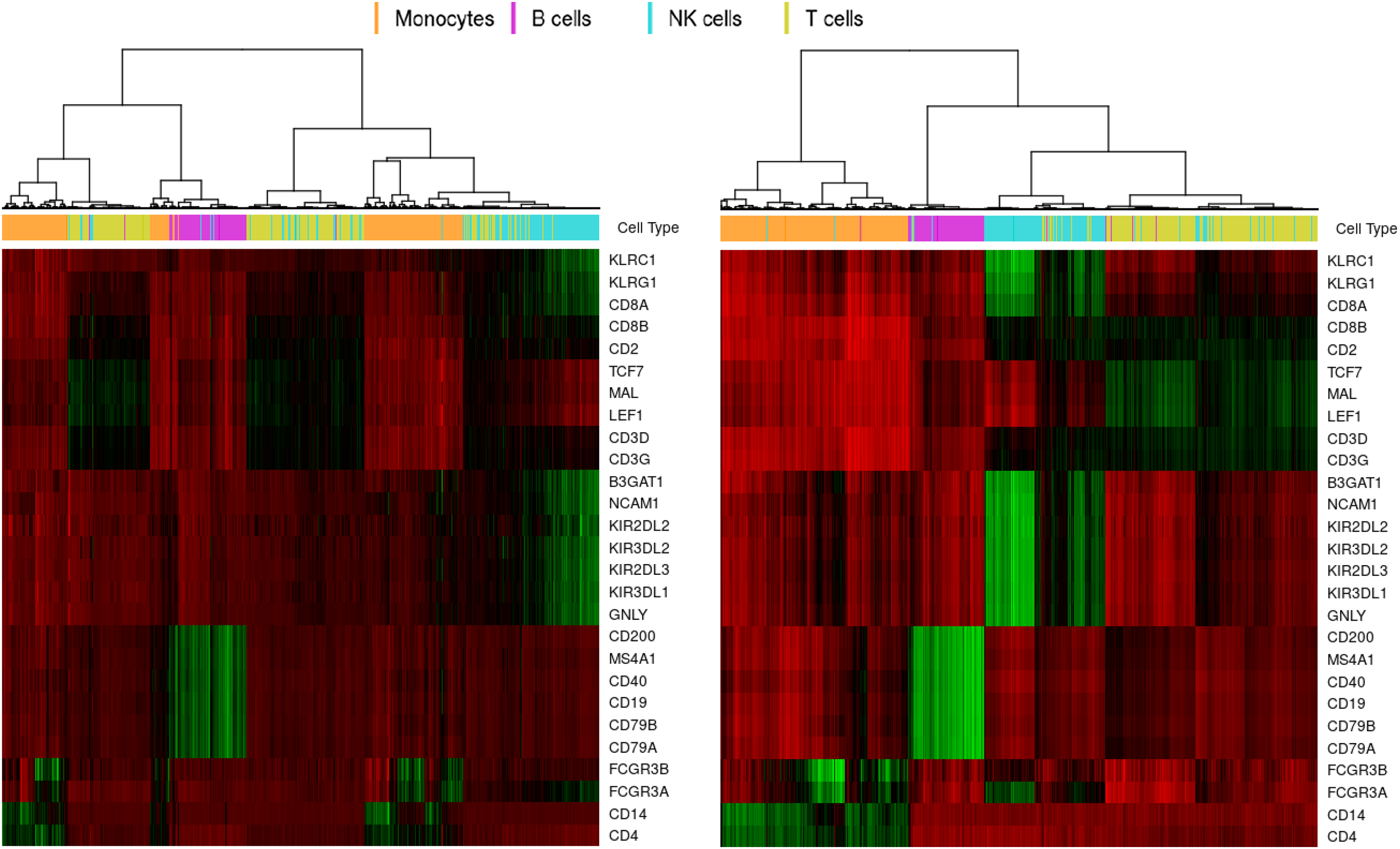
Next, we compared our method of dimension reduction with the method analogous to the one used in Zheng et al. (2017). With SVD, we calculate top 10 singular values (in pursuance of the L matrix rank) of the PBMC data matrix (A) using R irlba package. Then, the input data were approximated through the reduced 10-dimensional space. We perform the hierarchical clustering of all cells for the most characteristic marker genes per cell type (selected from the literature) on the described SVD-based approximation and the L matrices. The aim is to verify how well the dimensionality reduction preserves the most reliable biological information related to type-specific marker genes. It appeared that not only the L matrix guarantees more accurate clustering, but also it contains more pronounced differences of the signal between clusters of both cells and genes (Fig. 3).
Marker gene-based clustering comparison. The figure compares clustering of cells of known type with literature-based marker genes characterizing the analyzed types of PBMCs. The left panel is related to the signal represented in terms of the truncated SVD (10 highest singular values used). The right panel corresponds to the signal stored in the L matrix from trPCAL2. Top bars encode the original correlation-inferred cell types. Colors in the heatmap describe the activity level of a gene from lowest (red) through average (black) up to highest (green). SVD, singular value decomposition; trPCAL2, tRPCA with L2 regularization.
Monocyte subtypes and coexpression detection
The literature suggests existence of at least three subtypes of monocytes in PBMCs (Ziegler-Heitbrock et al., 2010) Their characterization can be based on the presence of CD14 (coded by CD14 gene) and CD16 (coded by FCGR3A, FCGR3B genes) clusters of differentiation: (1) the classical monocyte with high activity of CD14 (CD14++ FCGR3A−), (2) the intermediate monocyte with high activity of CD14 and low activity of FCGR3A (CD14++ FCGR3A+), and (3) the nonclassical monocyte with low activity of CD14 and coexpressed FCGR3A (CD14+ FCGR3A++).
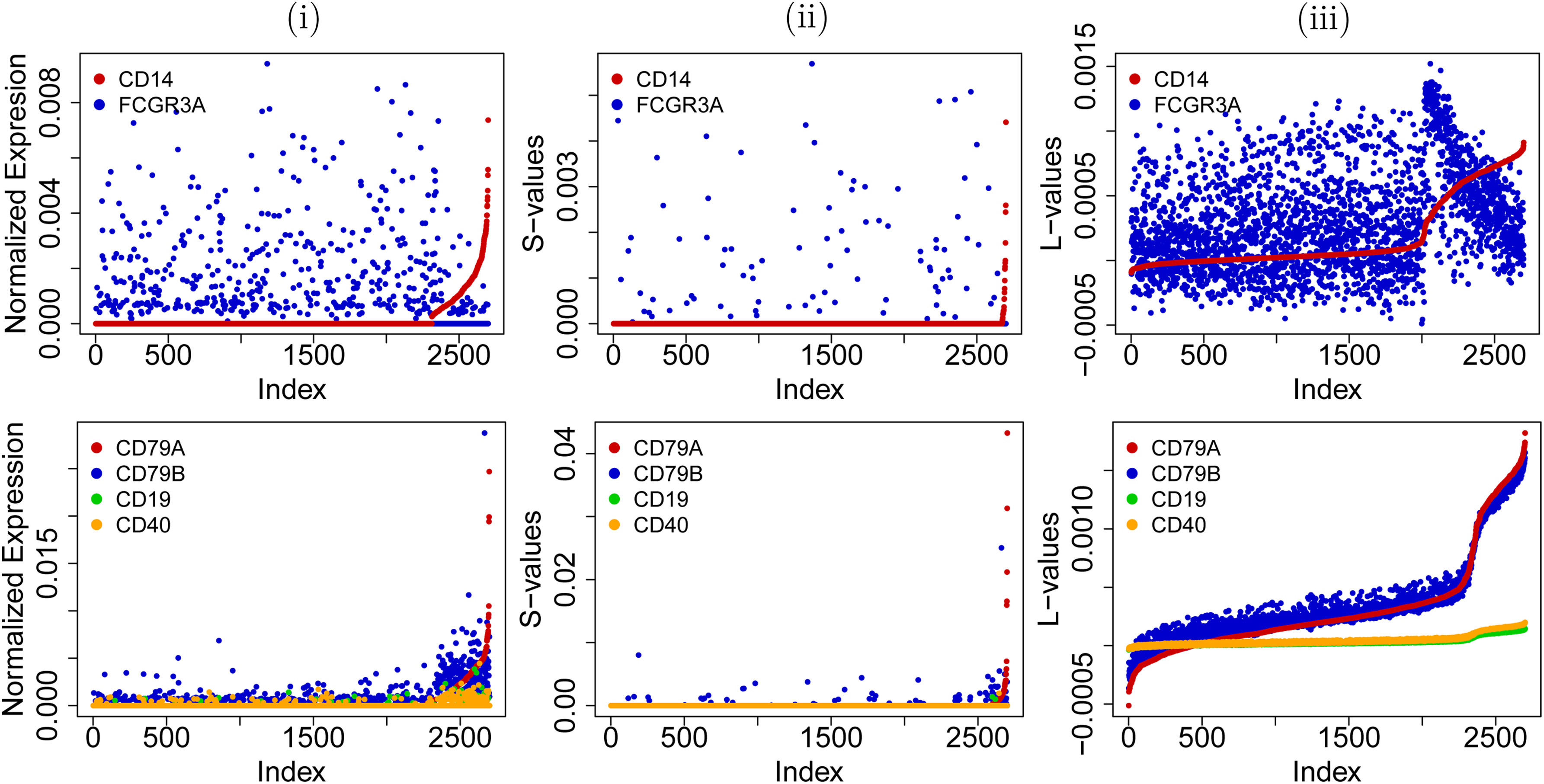
Interestingly, such classification of subtypes can be found using the low-rank signal from the L matrix (Fig. 4). The activity of CD14 is almost uniquely distributed among the cluster of monocyte cells and, simultaneously, the activity of FCGR3A changes with the gradient defining the cell subtype progression among all monocytes. Moreover, Figure 5 shows how the original expression values are distributed among decomposition matrices. The sparse peaks of activity are stored in S and the linear part in L. E matrix contained remaining noise of mean 0 and the standard deviation of order \documentclass{aastex}\usepackage{amsbsy}\usepackage{amsfonts}\usepackage{amssymb}\usepackage{bm}\usepackage{mathrsfs}\usepackage{pifont}\usepackage{stmaryrd}\usepackage{textcomp}\usepackage{portland, xspace}\usepackage{amsmath, amsxtra}\usepackage{upgreek}\pagestyle{empty}\DeclareMathSizes{10}{9}{7}{6}\begin{document}
$${10^{ - 4}}$$
\end{document} for both CD14 and FCGR3A.
CD14 and FCGR3A activity levels. Panels present the activity of monocytes marker genes. (a, b) Figures present the activity of CD14 and FCGR3A genes among all cells, respectively. The level of gene activity (lowest to highest) is spanned from red, through black, to green color scale.
Coexpression patterns. The distribution of the original expression levels among S and L matrices for marker genes of monocytes (top) and B cells (bottom). Consecutive panels present (i) the normalized log-transformed input data from A matrix, (ii) low-rank signal in L matrix, and (iii) sparse signal in S matrix. In each panel, cells (x-axis) are sorted by the activity level (y-axis) of first marker gene (CD14 for monocytes and CD79A for B cells).
In addition, the low-rank L matrix well tracks and recovers coexpression patterns between genes. Namely, the activity of B cells can be detected by the presence of CD79 heterodimer composed of CD79A and CD79B proteins (Chu and Arber, 2001). Their coexpression measured in terms of correlation was at the level of \documentclass{aastex}\usepackage{amsbsy}\usepackage{amsfonts}\usepackage{amssymb}\usepackage{bm}\usepackage{mathrsfs}\usepackage{pifont}\usepackage{stmaryrd}\usepackage{textcomp}\usepackage{portland, xspace}\usepackage{amsmath, amsxtra}\usepackage{upgreek}\pagestyle{empty}\DeclareMathSizes{10}{9}{7}{6}\begin{document}
$$0.227 ,$$
\end{document} whereas after the decomposition their low-rank signal had correlation of level \documentclass{aastex}\usepackage{amsbsy}\usepackage{amsfonts}\usepackage{amssymb}\usepackage{bm}\usepackage{mathrsfs}\usepackage{pifont}\usepackage{stmaryrd}\usepackage{textcomp}\usepackage{portland, xspace}\usepackage{amsmath, amsxtra}\usepackage{upgreek}\pagestyle{empty}\DeclareMathSizes{10}{9}{7}{6}\begin{document}
$$0.995$$
\end{document} (Fig. 5). Similarly, the correlation between FCGR3A and GNLY characterizing natural killer cells (Crinier et al., 2018) increased from \documentclass{aastex}\usepackage{amsbsy}\usepackage{amsfonts}\usepackage{amssymb}\usepackage{bm}\usepackage{mathrsfs}\usepackage{pifont}\usepackage{stmaryrd}\usepackage{textcomp}\usepackage{portland, xspace}\usepackage{amsmath, amsxtra}\usepackage{upgreek}\pagestyle{empty}\DeclareMathSizes{10}{9}{7}{6}\begin{document}
$$0.400$$
\end{document} to \documentclass{aastex}\usepackage{amsbsy}\usepackage{amsfonts}\usepackage{amssymb}\usepackage{bm}\usepackage{mathrsfs}\usepackage{pifont}\usepackage{stmaryrd}\usepackage{textcomp}\usepackage{portland, xspace}\usepackage{amsmath, amsxtra}\usepackage{upgreek}\pagestyle{empty}\DeclareMathSizes{10}{9}{7}{6}\begin{document}
$$0.949.$$
\end{document} Naturally, these observations are possible thanks to filtering out the sparse and noise signals. Nonetheless, this type of information is retrieved by the proposed method in an unsupervised manner, and may suggest new coexpression patterns.
Sparse signal interpretation
The presence of megakaryocytes in our PBMC data set, reported in the population of PBMCs sample from Zheng et al. (2017), was not evident using the low-rank L matrix, even though a small cluster of cells of unknown type was separated by t-SNE (Fig. 2) and an analogous cluster depicted in Figure 1a for 68,000 PBMCs data). Aiming in megakaryocytes detection, we performed the hierarchical clustering on the subset of unknown type cells and only genes that had at least one nonzero entry in the sparse S matrix. This resulted in recovery of a well-separated cluster of nine cells. Further analysis confirmed that the cluster is characterized by high overexpression of PF4 gene, which is a well-known marker for mature megakaryocytes (Adachi et al., 1991), in comparison with other unknown cell types.
Noise reduction and parameters
Finally, we want to discuss the importance of the noise matrix E and selection of \documentclass{aastex}\usepackage{amsbsy}\usepackage{amsfonts}\usepackage{amssymb}\usepackage{bm}\usepackage{mathrsfs}\usepackage{pifont}\usepackage{stmaryrd}\usepackage{textcomp}\usepackage{portland, xspace}\usepackage{amsmath, amsxtra}\usepackage{upgreek}\pagestyle{empty}\DeclareMathSizes{10}{9}{7}{6}\begin{document}
$${ \lambda _1}$$
\end{document} and \documentclass{aastex}\usepackage{amsbsy}\usepackage{amsfonts}\usepackage{amssymb}\usepackage{bm}\usepackage{mathrsfs}\usepackage{pifont}\usepackage{stmaryrd}\usepackage{textcomp}\usepackage{portland, xspace}\usepackage{amsmath, amsxtra}\usepackage{upgreek}\pagestyle{empty}\DeclareMathSizes{10}{9}{7}{6}\begin{document}
$${ \lambda _2}$$
\end{document} parameters. The final decomposition quality, in terms of information distribution among three matrices, is mainly based on the choice of these crucial parameters.
For the purpose of this study, we have set \documentclass{aastex}\usepackage{amsbsy}\usepackage{amsfonts}\usepackage{amssymb}\usepackage{bm}\usepackage{mathrsfs}\usepackage{pifont}\usepackage{stmaryrd}\usepackage{textcomp}\usepackage{portland, xspace}\usepackage{amsmath, amsxtra}\usepackage{upgreek}\pagestyle{empty}\DeclareMathSizes{10}{9}{7}{6}\begin{document}
$${ \lambda _1} = 0.016$$
\end{document} and \documentclass{aastex}\usepackage{amsbsy}\usepackage{amsfonts}\usepackage{amssymb}\usepackage{bm}\usepackage{mathrsfs}\usepackage{pifont}\usepackage{stmaryrd}\usepackage{textcomp}\usepackage{portland, xspace}\usepackage{amsmath, amsxtra}\usepackage{upgreek}\pagestyle{empty}\DeclareMathSizes{10}{9}{7}{6}\begin{document}
$${ \lambda _2} = 10.0 ,$$
\end{document} which resulted in \documentclass{aastex}\usepackage{amsbsy}\usepackage{amsfonts}\usepackage{amssymb}\usepackage{bm}\usepackage{mathrsfs}\usepackage{pifont}\usepackage{stmaryrd}\usepackage{textcomp}\usepackage{portland, xspace}\usepackage{amsmath, amsxtra}\usepackage{upgreek}\pagestyle{empty}\DeclareMathSizes{10}{9}{7}{6}\begin{document}
$$L + S + E$$
\end{document} decomposition with the following norms of the (vectorized) matrices: \documentclass{aastex}\usepackage{amsbsy}\usepackage{amsfonts}\usepackage{amssymb}\usepackage{bm}\usepackage{mathrsfs}\usepackage{pifont}\usepackage{stmaryrd}\usepackage{textcomp}\usepackage{portland, xspace}\usepackage{amsmath, amsxtra}\usepackage{upgreek}\pagestyle{empty}\DeclareMathSizes{10}{9}{7}{6}\begin{document}
$$\vert \vert \cdot { \vert \vert _*}: \,5.753 , \,60.289 , \,57.881;$$
\end{document}\documentclass{aastex}\usepackage{amsbsy}\usepackage{amsfonts}\usepackage{amssymb}\usepackage{bm}\usepackage{mathrsfs}\usepackage{pifont}\usepackage{stmaryrd}\usepackage{textcomp}\usepackage{portland, xspace}\usepackage{amsmath, amsxtra}\usepackage{upgreek}\pagestyle{empty}\DeclareMathSizes{10}{9}{7}{6}\begin{document}
$$\vert \vert \cdot { \vert \vert _1} \;: \, \;3398.162 , \,60.289 , \,2670.012;$$
\end{document}\documentclass{aastex}\usepackage{amsbsy}\usepackage{amsfonts}\usepackage{amssymb}\usepackage{bm}\usepackage{mathrsfs}\usepackage{pifont}\usepackage{stmaryrd}\usepackage{textcomp}\usepackage{portland, xspace}\usepackage{amsmath, amsxtra}\usepackage{upgreek}\pagestyle{empty}\DeclareMathSizes{10}{9}{7}{6}\begin{document}
$$\vert \vert \cdot { \vert \vert _2} \;: \; \,4.265 , \,2.826 , \,1.440$$
\end{document} (L, S, E, respectively).
Selection of the mentioned values was supported by the grid-based search through the parameter space. We have run tRPCAL2 decomposition on the PBMC data for 150 different, evenly distributed, pairs \documentclass{aastex}\usepackage{amsbsy}\usepackage{amsfonts}\usepackage{amssymb}\usepackage{bm}\usepackage{mathrsfs}\usepackage{pifont}\usepackage{stmaryrd}\usepackage{textcomp}\usepackage{portland, xspace}\usepackage{amsmath, amsxtra}\usepackage{upgreek}\pagestyle{empty}\DeclareMathSizes{10}{9}{7}{6}\begin{document}
$$( { \lambda _1} , { \lambda _2} ) \in \left[ {0.001 , 0.05} \right] \times \left[ {5 , 15} \right]$$
\end{document} setting \documentclass{aastex}\usepackage{amsbsy}\usepackage{amsfonts}\usepackage{amssymb}\usepackage{bm}\usepackage{mathrsfs}\usepackage{pifont}\usepackage{stmaryrd}\usepackage{textcomp}\usepackage{portland, xspace}\usepackage{amsmath, amsxtra}\usepackage{upgreek}\pagestyle{empty}\DeclareMathSizes{10}{9}{7}{6}\begin{document}
$${ \mu _0} = 147.28$$
\end{document} using the improved formula for the initiation of the \documentclass{aastex}\usepackage{amsbsy}\usepackage{amsfonts}\usepackage{amssymb}\usepackage{bm}\usepackage{mathrsfs}\usepackage{pifont}\usepackage{stmaryrd}\usepackage{textcomp}\usepackage{portland, xspace}\usepackage{amsmath, amsxtra}\usepackage{upgreek}\pagestyle{empty}\DeclareMathSizes{10}{9}{7}{6}\begin{document}
$${ \mu _0}$$
\end{document} parameter that takes into account the sparsity of an input data matrix A with k rows and l columns:
\documentclass{aastex}\usepackage{amsbsy}\usepackage{amsfonts}\usepackage{amssymb}\usepackage{bm}\usepackage{mathrsfs}\usepackage{pifont}\usepackage{stmaryrd}\usepackage{textcomp}\usepackage{portland, xspace}\usepackage{amsmath, amsxtra}\usepackage{upgreek}\pagestyle{empty}\DeclareMathSizes{10}{9}{7}{6}\begin{document}
\begin{align*}
{ \mu _0 } = { \frac { \vert \ { { a_ { i , j } } : \, { a_ { i , j } } \ne 0 \ } \vert } { 4 \cdot k \cdot l \cdot \sum \limits_ { i , j } \vert { a_ { i , j } } \vert } }
\end{align*}
\end{document}
The new formula is thus a ratio of the percent of nonzero values to four times the sum of absolute values in the data matrix. To determine the order of magnitude and search ranges for both parameters, we have made use of the theory described in Candès et al. (2011) as well as estimations based on the properties of the \documentclass{aastex}\usepackage{amsbsy}\usepackage{amsfonts}\usepackage{amssymb}\usepackage{bm}\usepackage{mathrsfs}\usepackage{pifont}\usepackage{stmaryrd}\usepackage{textcomp}\usepackage{portland, xspace}\usepackage{amsmath, amsxtra}\usepackage{upgreek}\pagestyle{empty}\DeclareMathSizes{10}{9}{7}{6}\begin{document}
$$A{A^T}$$
\end{document} matrix trace operator.
Since tRPCAL2 algorithm mixes L1 and L2 norms, which describe different mathematical properties and in this sense are incomparable, the final decomposition depends not only on relative or absolute values of chosen \documentclass{aastex}\usepackage{amsbsy}\usepackage{amsfonts}\usepackage{amssymb}\usepackage{bm}\usepackage{mathrsfs}\usepackage{pifont}\usepackage{stmaryrd}\usepackage{textcomp}\usepackage{portland, xspace}\usepackage{amsmath, amsxtra}\usepackage{upgreek}\pagestyle{empty}\DeclareMathSizes{10}{9}{7}{6}\begin{document}
$$\lambda _1 , \lambda_2$$
\end{document} parameters, but also on distributions of elements in the decomposed matrix. To approximate the relationship between \documentclass{aastex}\usepackage{amsbsy}\usepackage{amsfonts}\usepackage{amssymb}\usepackage{bm}\usepackage{mathrsfs}\usepackage{pifont}\usepackage{stmaryrd}\usepackage{textcomp}\usepackage{portland, xspace}\usepackage{amsmath, amsxtra}\usepackage{upgreek}\pagestyle{empty}\DeclareMathSizes{10}{9}{7}{6}\begin{document}
$${ \lambda _1}$$
\end{document} and \documentclass{aastex}\usepackage{amsbsy}\usepackage{amsfonts}\usepackage{amssymb}\usepackage{bm}\usepackage{mathrsfs}\usepackage{pifont}\usepackage{stmaryrd}\usepackage{textcomp}\usepackage{portland, xspace}\usepackage{amsmath, amsxtra}\usepackage{upgreek}\pagestyle{empty}\DeclareMathSizes{10}{9}{7}{6}\begin{document}
$${ \lambda _2}$$
\end{document} and their influence on the final composition of L, S, and E matrices, we summarized the results from simulation study and we conclude about properties such as the rank of the resulting L matrix, and relative and absolute sparsity of the S matrix (Fig. 6).
Properties of the algorithm. Each row presents value of some measurement as a function of product (left) and quotient (right) of \documentclass{aastex}\usepackage{amsbsy}\usepackage{amsfonts}\usepackage{amssymb}\usepackage{bm}\usepackage{mathrsfs}\usepackage{pifont}\usepackage{stmaryrd}\usepackage{textcomp}\usepackage{portland, xspace}\usepackage{amsmath, amsxtra}\usepackage{upgreek}\pagestyle{empty}\DeclareMathSizes{10}{9}{7}{6}\begin{document}
$$\lambda_1 , \lambda _2$$
\end{document} parameters, that tRPCAL2 was run with. (a) Norm values of each matrix and the objective function value. (b) The number of singular values of L matrix (top) and logarithm of sparsity (percent of nonzero matrix entries) of S matrix (bottom). On each plot, orange line corresponds to \documentclass{aastex}\usepackage{amsbsy}\usepackage{amsfonts}\usepackage{amssymb}\usepackage{bm}\usepackage{mathrsfs}\usepackage{pifont}\usepackage{stmaryrd}\usepackage{textcomp}\usepackage{portland, xspace}\usepackage{amsmath, amsxtra}\usepackage{upgreek}\pagestyle{empty}\DeclareMathSizes{10}{9}{7}{6}\begin{document}
$$\lambda_1 , \lambda _2$$
\end{document} parameters finally used in our study.
First, we systematize the boundary behaviors of the algorithm. Namely, when \documentclass{aastex}\usepackage{amsbsy}\usepackage{amsfonts}\usepackage{amssymb}\usepackage{bm}\usepackage{mathrsfs}\usepackage{pifont}\usepackage{stmaryrd}\usepackage{textcomp}\usepackage{portland, xspace}\usepackage{amsmath, amsxtra}\usepackage{upgreek}\pagestyle{empty}\DeclareMathSizes{10}{9}{7}{6}\begin{document}
$${ \lambda _1 , \lambda _2} \to \infty$$
\end{document} the decomposition will result in \documentclass{aastex}\usepackage{amsbsy}\usepackage{amsfonts}\usepackage{amssymb}\usepackage{bm}\usepackage{mathrsfs}\usepackage{pifont}\usepackage{stmaryrd}\usepackage{textcomp}\usepackage{portland, xspace}\usepackage{amsmath, amsxtra}\usepackage{upgreek}\pagestyle{empty}\DeclareMathSizes{10}{9}{7}{6}\begin{document}
$$L = A , S = E = 0.$$
\end{document} Next, for fixed \documentclass{aastex}\usepackage{amsbsy}\usepackage{amsfonts}\usepackage{amssymb}\usepackage{bm}\usepackage{mathrsfs}\usepackage{pifont}\usepackage{stmaryrd}\usepackage{textcomp}\usepackage{portland, xspace}\usepackage{amsmath, amsxtra}\usepackage{upgreek}\pagestyle{empty}\DeclareMathSizes{10}{9}{7}{6}\begin{document}
$${ \lambda _1}$$
\end{document} and \documentclass{aastex}\usepackage{amsbsy}\usepackage{amsfonts}\usepackage{amssymb}\usepackage{bm}\usepackage{mathrsfs}\usepackage{pifont}\usepackage{stmaryrd}\usepackage{textcomp}\usepackage{portland, xspace}\usepackage{amsmath, amsxtra}\usepackage{upgreek}\pagestyle{empty}\DeclareMathSizes{10}{9}{7}{6}\begin{document}
$${ \lambda _2} \to 0$$
\end{document} the information shifts to E matrix and \documentclass{aastex}\usepackage{amsbsy}\usepackage{amsfonts}\usepackage{amssymb}\usepackage{bm}\usepackage{mathrsfs}\usepackage{pifont}\usepackage{stmaryrd}\usepackage{textcomp}\usepackage{portland, xspace}\usepackage{amsmath, amsxtra}\usepackage{upgreek}\pagestyle{empty}\DeclareMathSizes{10}{9}{7}{6}\begin{document}
$$E = A , L = S = 0.$$
\end{document} Similarly, fixed \documentclass{aastex}\usepackage{amsbsy}\usepackage{amsfonts}\usepackage{amssymb}\usepackage{bm}\usepackage{mathrsfs}\usepackage{pifont}\usepackage{stmaryrd}\usepackage{textcomp}\usepackage{portland, xspace}\usepackage{amsmath, amsxtra}\usepackage{upgreek}\pagestyle{empty}\DeclareMathSizes{10}{9}{7}{6}\begin{document}
$${ \lambda _2}$$
\end{document} and \documentclass{aastex}\usepackage{amsbsy}\usepackage{amsfonts}\usepackage{amssymb}\usepackage{bm}\usepackage{mathrsfs}\usepackage{pifont}\usepackage{stmaryrd}\usepackage{textcomp}\usepackage{portland, xspace}\usepackage{amsmath, amsxtra}\usepackage{upgreek}\pagestyle{empty}\DeclareMathSizes{10}{9}{7}{6}\begin{document}
$${ \lambda _1} \to 0$$
\end{document} gives \documentclass{aastex}\usepackage{amsbsy}\usepackage{amsfonts}\usepackage{amssymb}\usepackage{bm}\usepackage{mathrsfs}\usepackage{pifont}\usepackage{stmaryrd}\usepackage{textcomp}\usepackage{portland, xspace}\usepackage{amsmath, amsxtra}\usepackage{upgreek}\pagestyle{empty}\DeclareMathSizes{10}{9}{7}{6}\begin{document}
$$S = A , L = E = 0$$
\end{document} (Fig. 6a). Although intuitive, these observations depend on different convergence rate, and thus flow of the information among resulting matrices. Here, based on the described set of simulations, we indicate several observations regarding signal distribution (Fig. 6b): (1) the rank of matrix L increases (2) sublinearly as a function of \documentclass{aastex}\usepackage{amsbsy}\usepackage{amsfonts}\usepackage{amssymb}\usepackage{bm}\usepackage{mathrsfs}\usepackage{pifont}\usepackage{stmaryrd}\usepackage{textcomp}\usepackage{portland, xspace}\usepackage{amsmath, amsxtra}\usepackage{upgreek}\pagestyle{empty}\DeclareMathSizes{10}{9}{7}{6}\begin{document}
$${ \lambda _1}$$
\end{document} and fixed \documentclass{aastex}\usepackage{amsbsy}\usepackage{amsfonts}\usepackage{amssymb}\usepackage{bm}\usepackage{mathrsfs}\usepackage{pifont}\usepackage{stmaryrd}\usepackage{textcomp}\usepackage{portland, xspace}\usepackage{amsmath, amsxtra}\usepackage{upgreek}\pagestyle{empty}\DeclareMathSizes{10}{9}{7}{6}\begin{document}
$${ \lambda _2}$$
\end{document}; (3) polynomially as a function of \documentclass{aastex}\usepackage{amsbsy}\usepackage{amsfonts}\usepackage{amssymb}\usepackage{bm}\usepackage{mathrsfs}\usepackage{pifont}\usepackage{stmaryrd}\usepackage{textcomp}\usepackage{portland, xspace}\usepackage{amsmath, amsxtra}\usepackage{upgreek}\pagestyle{empty}\DeclareMathSizes{10}{9}{7}{6}\begin{document}
$${ \lambda _2}$$
\end{document} and fixed \documentclass{aastex}\usepackage{amsbsy}\usepackage{amsfonts}\usepackage{amssymb}\usepackage{bm}\usepackage{mathrsfs}\usepackage{pifont}\usepackage{stmaryrd}\usepackage{textcomp}\usepackage{portland, xspace}\usepackage{amsmath, amsxtra}\usepackage{upgreek}\pagestyle{empty}\DeclareMathSizes{10}{9}{7}{6}\begin{document}
$${ \lambda _1}$$
\end{document}; (4) for fixed \documentclass{aastex}\usepackage{amsbsy}\usepackage{amsfonts}\usepackage{amssymb}\usepackage{bm}\usepackage{mathrsfs}\usepackage{pifont}\usepackage{stmaryrd}\usepackage{textcomp}\usepackage{portland, xspace}\usepackage{amsmath, amsxtra}\usepackage{upgreek}\pagestyle{empty}\DeclareMathSizes{10}{9}{7}{6}\begin{document}
$${ \lambda _2}$$
\end{document} sparsity (percent of nonzero elements) of S decreases exponentially as a function of \documentclass{aastex}\usepackage{amsbsy}\usepackage{amsfonts}\usepackage{amssymb}\usepackage{bm}\usepackage{mathrsfs}\usepackage{pifont}\usepackage{stmaryrd}\usepackage{textcomp}\usepackage{portland, xspace}\usepackage{amsmath, amsxtra}\usepackage{upgreek}\pagestyle{empty}\DeclareMathSizes{10}{9}{7}{6}\begin{document}
$${ \lambda _1}.$$
\end{document}
Finally, we observed that the distribution of E elements is a mixture of zero-centered Gaussian and low-variance Gaussian concentrated around non-negative \documentclass{aastex}\usepackage{amsbsy}\usepackage{amsfonts}\usepackage{amssymb}\usepackage{bm}\usepackage{mathrsfs}\usepackage{pifont}\usepackage{stmaryrd}\usepackage{textcomp}\usepackage{portland, xspace}\usepackage{amsmath, amsxtra}\usepackage{upgreek}\pagestyle{empty}\DeclareMathSizes{10}{9}{7}{6}\begin{document}
$${ \lambda _2}$$
\end{document}-dependent value. We reason that since tRPCAL2 is an optimization of linear combination of norms, E matrix captures parts of low-rank and sparse components bringing such mixture. One way to overcome this effect was described in Zhang et al. (2016) through their truncated nuclear norm minimization for RPCA.
More formal investigation of the tRPCAL2 theoretical properties with respect to \documentclass{aastex}\usepackage{amsbsy}\usepackage{amsfonts}\usepackage{amssymb}\usepackage{bm}\usepackage{mathrsfs}\usepackage{pifont}\usepackage{stmaryrd}\usepackage{textcomp}\usepackage{portland, xspace}\usepackage{amsmath, amsxtra}\usepackage{upgreek}\pagestyle{empty}\DeclareMathSizes{10}{9}{7}{6}\begin{document}
$${ \lambda _1} , { \lambda _2}$$
\end{document} and L, S, E matrices could be of high interest in terms of future research.
5. Conclusions
In this article, we introduce an extension of RPCA. We propose to decompose the input matrix into low-rank L, sparse S, and noise E components. Thanks to the reduction of noise using the L2 penalty, we restore the inner structure of the matrix. Our results suggest that our algorithms may better approximate the underlying systematic variation in the input data, as well as recognize the sparse perturbation signal of the data. We present the case study based on the scRNA-seq data from 2700 PBMCs. The method provides relatively fast and accurate dimension reduction and clustering of the high-dimensional data detecting different subtypes within a given cell type, coexpression patterns, and novel subtypes.
One possible direction for the further research is to derive precise formulas for \documentclass{aastex}\usepackage{amsbsy}\usepackage{amsfonts}\usepackage{amssymb}\usepackage{bm}\usepackage{mathrsfs}\usepackage{pifont}\usepackage{stmaryrd}\usepackage{textcomp}\usepackage{portland, xspace}\usepackage{amsmath, amsxtra}\usepackage{upgreek}\pagestyle{empty}\DeclareMathSizes{10}{9}{7}{6}\begin{document}
$${ \lambda _1}$$
\end{document} and \documentclass{aastex}\usepackage{amsbsy}\usepackage{amsfonts}\usepackage{amssymb}\usepackage{bm}\usepackage{mathrsfs}\usepackage{pifont}\usepackage{stmaryrd}\usepackage{textcomp}\usepackage{portland, xspace}\usepackage{amsmath, amsxtra}\usepackage{upgreek}\pagestyle{empty}\DeclareMathSizes{10}{9}{7}{6}\begin{document}
$${ \lambda _2}$$
\end{document} parameters that guarantee optimal solutions of the decomposition problem. So far, simulation-based selection of the parameters is time consuming. Ideally, a \documentclass{aastex}\usepackage{amsbsy}\usepackage{amsfonts}\usepackage{amssymb}\usepackage{bm}\usepackage{mathrsfs}\usepackage{pifont}\usepackage{stmaryrd}\usepackage{textcomp}\usepackage{portland, xspace}\usepackage{amsmath, amsxtra}\usepackage{upgreek}\pagestyle{empty}\DeclareMathSizes{10}{9}{7}{6}\begin{document}
$$\lambda_1 , \lambda _2$$
\end{document} parameters selection method would result with the most natural \documentclass{aastex}\usepackage{amsbsy}\usepackage{amsfonts}\usepackage{amssymb}\usepackage{bm}\usepackage{mathrsfs}\usepackage{pifont}\usepackage{stmaryrd}\usepackage{textcomp}\usepackage{portland, xspace}\usepackage{amsmath, amsxtra}\usepackage{upgreek}\pagestyle{empty}\DeclareMathSizes{10}{9}{7}{6}\begin{document}
$$L + S + E$$
\end{document} decomposition, taking into account user's expectations in terms of, for example, Bayesian priors to relative magnitudes, and to other components' statistics. The applicability of our method to other types of data, we also see as a promising direction of a further research. Preliminary results of video and image analysis, not described in this article, suggest that the method can be successfully harnessed in the field of video surveillance and image analysis. The current implementation of the tRPCAL2 algorithm is available online: https://github.com/macieksk/rpca as a development R package.
Footnotes
Acknowledgments
This study was partially supported by the Polish National Science Centre grant nos. 2016/21/N/ST6/01507 and 2016/23/D/ST6/03613. The authors thank B. Miasojedow, PhD, for comments and suggestions. Preliminary version of this study was published as an extended abstract in proceedings of ISBRA 2018 Conference, Beijing, China (LNCS vol. 10847).
Author Disclosure Statement
The authors declare there are no competing financial interests.
References
1.
AdachiM., RyoR., SatoT., et al.1991. Platelet factor 4 gene expression in a human megakaryocytic leukemia cell line (CMK) and its differentiated subclone (CMK11-5). Exp. Hematol. 19, 923–927.
2.
BaglamaJ., ReichelL., and LewisB.W.2018. irlba: Fast Truncated Singular Value Decomposition and Principal Components Analysis for Large Dense and Sparse Matrices. R package version 2.3.2. https://cran.r-project.org/web/packages/irlba/ Accessed January7, 2019.
3.
BartenhagenC. 2018. RDRToolbox: A package for nonlinear dimension reduction with Isomap and LLE. R package version 1.32.0. https://bioconductor.org/packages/RDRToolbox/ Accessed January7, 2019.
4.
BartholomewD.J., KnottM., and MoustakiI.2011. Latent Variable Models and Factor Analysis: A Unified Approach. Wiley Series in Probability and Statistics, Chichester, West Sussex.
5.
BasuS., CampbellH.M., DittelB.N., et al.2010. Purification of specific cell population by fluorescence activated cell sorting (FACS). J. Vis. Exp. 10, 41.
6.
CandèsE.J., LiX., MaY., et al.2011. Robust principal component analysis?. J. ACM, 58, 11:1–11:37.
7.
ChuL.F., LengN., ZhangJ., et al.2016. Single-cell RNA-seq reveals novel regulators of human embryonic stem cell differentiation to definitive endoderm. Genome Biol. 17, 173.
8.
ChuP.G., and ArberD.A.2001. CD79: A review. Appl. Immunohistochem. Mol. Morphol. 9, 97–106.
9.
ChungN.C., and StoreyJ.D.2015. Statistical significance of variables driving systematic variation in high-dimensional data. Bioinformatics, 31, 545–554.
10.
CrinierA., MilpiedP., EscaliereB., et al.2018. High-dimensional single-cell analysis identifies organ-specific signatures and conserved NK cell subsets in humans and mice. Immunity, 49, 971–986.
11.
GogolewskiK., WronowskaW., LechA., et al.2017. Inferring molecular processes heterogeneity from transcriptional data. Biomed. Res. Int. 2017, id–6961786.
12.
HartiganJ.A., and WongM.A.1979. Algorithm AS 136: A K-Means clustering algorithm. Appl. Stat. 28, 100–108.
13.
IlicicT., KimJ.K., KolodziejczykA.A., et al.2016. Classification of low quality cells from single-cell RNA-seq data. Genome Biol. 17, 29.
JolliffeI.T. 2002. Principal Component Analysis. Springer Verlag, NewYork, NY.
16.
LeeD.D., and SeungH.S.1999. Learning the parts of objects by non-negative matrix factorization. Nature, 401, 788–791.
17.
LeekJ.T.2010. Asymptotic conditional singular value decomposition for high-dimensional genomic data. Biometrics, 67, 344–352.
18.
LloydS.P.1982. Least squares quantization in PCM. IEEE Trans. Inf. Theory, 28, 129–137.
19.
MacqueenJ.1967. Some methods for classification and analysis of multivariate observations. In Proceedings of the 5-th Berkeley Symposium on Mathematical Statistics and Probability. pp. 281–297. University of California Press, Berkeley, CA.
NovelliG., CiccacciC., BorgianiP., et al.2008. Genetic tests and genomic biomarkers: Regulation, qualification and validation. Clin. Cases Miner. Bone Metab. 5, 149–154.
22.
OhkawaT., SekiS., DobashiH., et al.2001. Systematic characterization of human CD8+ T cells with natural killer cell markers in comparison with natural killer cells and normal CD8+ T cells. Immunology, 103, 281–290.
23.
RamazzottiD., WangB., and De SanoL.2018. SIMLR: Single-cell Interpretation via Multi-kernel LeaRning. R package version 1.8.0. https://bioconductor.org/packages/SIMLR/ Accessed January7, 2019.
24.
RamsköldD., LuoS., WangY.C., et al.2012. Full-length mRNA-Seq from single-cell levels of RNA and individual circulating tumor cells. Nat. Biotechnol. 30, 777–782.
25.
SykulskiM. 2015. rpca: RobustPCA: Decompose a Matrix into Low-Rank and Sparse Components. R package version 0.2.3. https://cran.r-project.org/web/packages/rpca/ Accessed January7, 2019.
26.
UsoskinD., FurlanA., IslamS., et al.2015. Unbiased classification of sensory neuron types by large-scale single-cell RNA sequencing. Nat. Neurosci. 18, 145–153.
27.
van der MaatenL.2014. Accelerating t-SNE using tree-based algorithms. J. Mach. Learn. Res. 15, 3221–3245.
28.
WangY., and NavinN.E.2015. Advances and applications of single-cell sequencing technologies. Mol. Cell, 58, 598–609.
29.
WillsQ.F., LivakK.J., TippingA.J., et al.2013. Single-cell gene expression analysis reveals genetic associations masked in whole-tissue experiments. Nat. Biotechnol. 31, 748–752.
30.
WittenD.M., TibshiraniR., and HastieT.2009. A penalized matrix decomposition, with applications to sparse principal components and canonical correlation analysis. Biostatistics, 10, 515–534.
31.
YuanX., and YangJ.2009. Sparse and low-rank matrix decomposition via alternating direction methods. Available at: optimization-online.org. Accessed January7, 2019.
32.
ZhangY., GuoJ., ZhaoJ., et al.2016. Robust principal component analysis via truncated nuclear norm minimization. J. Shang. Jiaot. Uni. 21, 576–583.
33.
ZhengG.X., TerryJ.M., BelgraderP., et al.2017. Massively parallel digital transcriptional profiling of single cells. Nat. Commun. 8, 14049.
34.
Ziegler-HeitbrockL., AncutaP., CroweS., et al.2010. Nomenclature of monocytes and dendritic cells in blood. Blood, 116, 16, 74–80.
35.
ZouH., HastieT., and TibshiraniR.2006. Sparse principal component analysis. JCGS, 15, 262–286.