RN + : A Novel Biclustering Algorithm for Analysis of Gene Expression Data Using Protein

Abstract

Biclustering is a process of finding groups of genes that behave similarly under a subset of conditions. In this article, we propose an efficient biclustering algorithm, namely RN⁺, to identify biologically meaningful biclusters in gene expression data. The RN⁺ algorithm finds biologically meaningful biclusters through a novel gene filtering using protein–protein interaction network, gene searching, gene grouping, and queuing process. It also efficiently removes duplicate biclusters. We tested the proposed RN⁺ on five real microarray datasets, and compared its performance with seven competitive biclustering algorithms. The experimental results show that RN⁺ efficiently finds functionally enriched and biologically meaningful biclusters for large gene expression datasets, and outperforms the other tested biclustering algorithms on real datasets.

1. Introduction

Microarray data are a two-dimensional matrix of gene expression levels measured under different conditions (Saullo et al., 2015). The data can be viewed as an m × n matrix with m genes (rows) and n conditions (columns), in which each entry represents the expression level of a gene under each condition (Wang et al., 2016). For many analyses, it is important to find clusters of genes that have the same function. Clustering has been an important tool for analyzing microarray data. Conventional clustering methods such as K-means have found identified genes or samples that are functionally related under specific conditions (Li et al., 2012). Some genes are not coexpressed under all conditions and may be similar only in a subset of experimental conditions (Li et al., 2012).

Biclustering is a process of identifying groups of genes that behave similarly under a specific subset of conditions. However, finding biclusters in microarray data is difficult because the number of potential biclusters increases as the number of genes and the number of samples increase (Bhattacharya and Cui, 2017). Biclustering has been proven to be a non-deterministic polynomial time (NP)-hard problem (Ahn et al., 2011). Many biclustering algorithms therefore use heuristic methods, and their solutions may be suboptimal (Ahn et al., 2011). There are advantages and disadvantages to each algorithm, depending on the pattern of biclusters. This article proposes an algorithm, RN⁺, which is a variant of the RN clustering algorithm described in Ahn et al. (2011), and which tries to find as many functionally associated biclusters as possible. We tested and compared RN⁺ with seven competitive biclustering algorithms on real datasets. The results show that RN⁺ outperformed other biclustering algorithms in terms of both the number of enriched biclusters and the percentage of biologically meaningful biclusters.

2. Related Work

Existing biclustering algorithms can be divided into several categories. The first category is pattern-based biclustering. This approach tries to find strictly additive or multiplicative patterns. However, many of pattern-based biclustering algorithms are exponential with respect to the size of the microarray data or the noise level of the microarray data (Xu et al., 2006). Therefore, this approach is not practical for large datasets. Moreover, these pattern-based algorithms tend to find too many biclusters that are only slightly different. The second category is tendency-based biclustering, algorithms that identify Order-Preserving Submatrices (OPSMs) and use them to find biclusters (Ahn et al., 2011). The OPSM belongs to this category (Ben-Dor et al., 2003). It was reported that the OPSM has shown good gene ontology (GO) validation results (Ahn et al., 2011). However, the OPSM finds only one bicluster with the best results every time it is executed, so multiple biclusters may not be identified. This algorithm also risks missing hidden patterns in microarray data (Ahn et al., 2011).

Another category is a divide-and-conquer algorithm. These algorithms divide a problem into small subproblems, solve each subproblem recursively, and then combine subsolutions into one solution. The Binary Inclusion-Maximal Biclustering Algorithm (Bimax) is an example of this category. It finds all submatrices whose entries are equal to 1 in a binary matrix. It has been reported that Bimax performs well on certain patterns, such as upregulated biclusters (Eren et al., 2012). Another algorithm, Statistical-Algorithmic Method for Bicluster Analysis (SAMBA), employs a statistical model of biclusters and develops combinatorial methods for biclustering large datasets. The SAMBA enumerates all the possible biclusters and showed robustness with respect to noise. Another algorithm, Qualitative Biclustering (QUBIC), employs statistical models to find all statistically significant biclusters. In addition, the iterative signature algorithm (ISA) (Bergmann et al., 2003) and Sequential row-based biclustering algorithm for analysis of gene expression data (UniBIC) (Yun and Yi, 2013) biclustering algorithms have been described for finding biclusters in the microarray data.

3. Method

3.1. Notations

In this article, we use the following terminologies:

g₀, g₁,… g_m-1: genes

s₀, s₁, …. s_n-1: samples

p-BCS: bicluster candidate set (BCS) consisting of p samples

\documentclass{aastex}\usepackage{amsbsy}\usepackage{amsfonts}\usepackage{amssymb}\usepackage{bm}\usepackage{mathrsfs}\usepackage{pifont}\usepackage{stmaryrd}\usepackage{textcomp}\usepackage{portland, xspace}\usepackage{amsmath, amsxtra}\usepackage{upgreek}\pagestyle{empty}\DeclareMathSizes{10}{9}{7}{6}\begin{document} $$d_{ij}^k:$$ \end{document} the expression value of the j^th sample in the sample set—the expression value of the i^th sample in the sample set in the gene g_k

deg_th: user-specified degree threshold

dist_th: user-specified distance threshold

edge_th: user-specified edge threshold

mns: user-specified minimum number of samples in BCS

mng: user-specified minimum number of genes in BCS

st: user-specified similarity threshold between two BCSs

3.2. RN⁺ algorithm

The RN⁺ algorithm is composed of five main steps: 1.

Gene filtering using protein–protein interaction (PPI) network data

Find 2-BCS (bicluster candidate set);

Obtain (p + 1)-BCSs from p-BCSs;

Single priority queuing;

Remove duplicate BCSs

3.2.1. Step 1: Gene filtering using gene network data

The goal of our first step is to find genes that are closely related to each other using the PPI network data. PPI network data can be represented as a graph. Each node represents a gene, and nodes are connected by undirected edges. We set the weight of the edges to 1. Step 1 is composed of three substeps: (1) remove genes with a high degree, (2) create subgraphs (gene sets) for each gene and remove duplicate gene sets, and (3) remove relatively sparse subgraphs, which contain few edges. First, we remove high-degree genes from the graph, since genes that are not highly related may have a short distance from other genes due to the presence of high-degree genes. The distance between two genes is the number of edges in the shortest path between them. Let the degree of a gene v and the total number of genes (vertices) in the graph be deg(v) and M, respectively. We remove edges of high-degree genes, which do not satisfy the following equation: \documentclass{aastex}\usepackage{amsbsy}\usepackage{amsfonts}\usepackage{amssymb}\usepackage{bm}\usepackage{mathrsfs}\usepackage{pifont}\usepackage{stmaryrd}\usepackage{textcomp}\usepackage{portland, xspace}\usepackage{amsmath, amsxtra}\usepackage{upgreek}\pagestyle{empty}\DeclareMathSizes{10}{9}{7}{6}\begin{document} \begin{align*} \frac { { { \rm { deg } } \left( v \right) } } { M } < deg \;\_\;th. \tag { 1 } \end{align*} \end{document}

Second, to find a dense subgraph for each gene, we set a parameter called dist_th. We visit all genes and construct subgraphs for each gene, whose distance from the current gene is less than dist_th. When we create subgraphs by going through all the genes in this way, the number of subgraphs becomes equal to the number of genes, and there are many subgraphs that are similar to each other. We then remove duplicate subgraphs. If the overlapping ratio of the two subgraphs intersecting each other exceeds st, then the subgraph with the smaller size is removed to eliminate duplicate gene sets. For example, if st is 0.7 and two subgraphs are {g₃, g₄, g₉, g₁₃} and {g₃, g₄, g₉}, the overlapping ratio is \documentclass{aastex}\usepackage{amsbsy}\usepackage{amsfonts}\usepackage{amssymb}\usepackage{bm}\usepackage{mathrsfs}\usepackage{pifont}\usepackage{stmaryrd}\usepackage{textcomp}\usepackage{portland, xspace}\usepackage{amsmath, amsxtra}\usepackage{upgreek}\pagestyle{empty}\DeclareMathSizes{10}{9}{7}{6}\begin{document} $$0.75$$ \end{document} . Thus, {g₃, g₄, g₉} is removed, and {g₃, g₄, g₉, g₁₃} remains.

The presence of many edges in any of the remaining subgraphs indicates that the genes belonging to the subgraph are highly related. The maximum number of edges in the i^th subgraph is \documentclass{aastex}\usepackage{amsbsy}\usepackage{amsfonts}\usepackage{amssymb}\usepackage{bm}\usepackage{mathrsfs}\usepackage{pifont}\usepackage{stmaryrd}\usepackage{textcomp}\usepackage{portland, xspace}\usepackage{amsmath, amsxtra}\usepackage{upgreek}\pagestyle{empty}\DeclareMathSizes{10}{9}{7}{6}\begin{document} $$\frac { { { M_i } \left( { { M_i } - 1 } \right) } } { 2 } $$ \end{document} , when the total number of vertices in the subgraph is M_i. Let the total number of edges in the i^th subgraph be E_i. We remove relatively sparse subgraphs, which do not satisfy the following equation: \documentclass{aastex}\usepackage{amsbsy}\usepackage{amsfonts}\usepackage{amssymb}\usepackage{bm}\usepackage{mathrsfs}\usepackage{pifont}\usepackage{stmaryrd}\usepackage{textcomp}\usepackage{portland, xspace}\usepackage{amsmath, amsxtra}\usepackage{upgreek}\pagestyle{empty}\DeclareMathSizes{10}{9}{7}{6}\begin{document} \begin{align*} \frac { 2 } { { { M_i } \left( { { M_i } - 1 } \right) { \rm { \; } } } } { E_i } > edge \_th. \tag { 2 } \end{align*} \end{document}

Figure 1 shows a toy example. An initial graph with 13 genes is shown in Figure 1a. For this example, we use the following parameters: deg_th = 0.5, dist_th = 2, and edge_th = 0.4, st = 0.7, and mng = 3. First, the edges of g₁ are removed since it does not satisfy (1). The output graph after removing a large-degree gene, in this case g₁, is shown in Figure 1b. Then, a total of 13 subgraphs for each gene are generated. Three subgraphs, {g₈, g₁₂}, {g₃, g₄, g₉, g₁₃}, and {g₅, g₆, g₇, g₁₀, g₁₁}, remain after removing duplicate gene sets and, additionally, {g₈, g₁₂} is removed, since the number of genes comparing it is less than mng (Fig. 1c). Finally, only {g₅, g₆, g₇, g₁₀, g₁₁} remains, and {g₃, g₄, g₉, g₁₃} is removed since it does not satisfy (2).

FIG. 1.

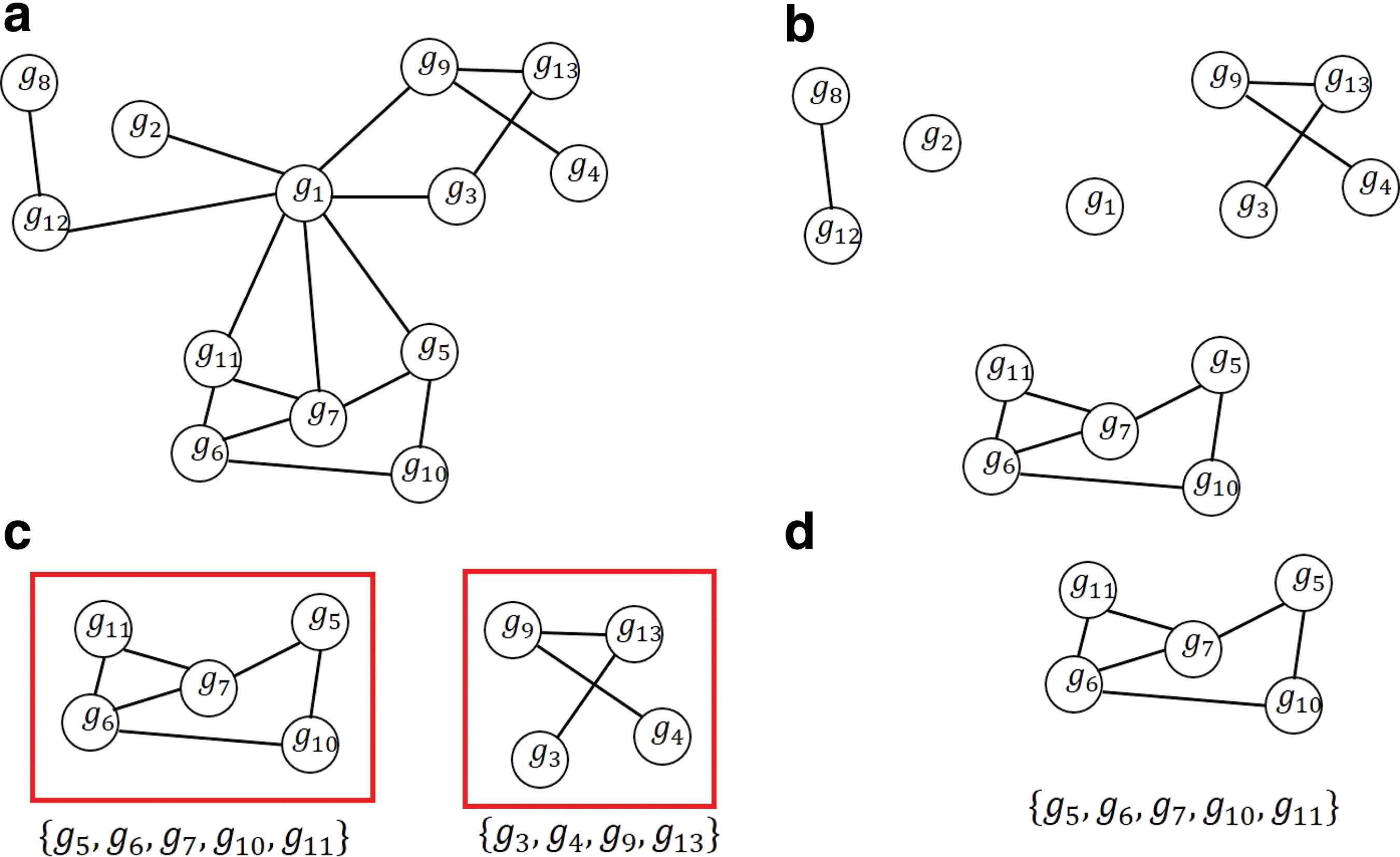
Toy example of gene filtering using protein–protein interaction network data when deg_th = 0.5, dist_th = 2, edge_th = 0.5, st = 0.7, and mng = 3. (a) An initial gene graph with 13 genes; (b) the output graph after removing a large-degree gene, g1; (c) two output subgraphs after removing duplicate gene sets; and (d) output subgraph after removing a relatively sparse subgraph.

3.2.2. Step 2: Find 2-BCS

If the number of samples in the microarray data is n, extract all possible two-sample pairs from these samples to generate a 2-BCS for all genes, which passed step 1. So, a p-BCS is a small bicluster candidate with p-samples for being expanded to a larger bicluster. If the expression values in other samples are the same as those of a specific gene, these sample pairs are excluded when making a 2-BCS. This approach creates a maximum number of possible cases of C (n, 2) when generating 2-BCSs. However, any 2-BCS that cannot meet the mns condition, which is specified by the user, is not created. For example, if there are four samples (n = 4) in a microarray dataset, s₀, s₁, s₂, and s₃, then a total of six 2-BCSs are possible, {s₀, s₁}, {s₀, s₂}, {s₀, s₃}, {s₁, s₂}, {s₁, s₃}, and {s₂, s₃}. However, if mns = 3, {s₁, s₃}, {s₂, s₃} that cannot be further expanded are not generated.

3.2.3. Step 3: Obtain (p + 1)-BCSs from p-BCSs

When expanding from p-BCSs to (p + 1)-BCSs, we select the last sample of each p-BCS sample set as the sample to be expanded. For example, when making 3-BCS from 2-BCS, if the samples in 2-BCS are {s₁, s₂}, then the last sample is s₂, so we select s₃ as the next sample to expand. That is, (p + 1)-BCS is obtained from p-BCS using breadth-first search (BFS) as shown in Figure 2.

FIG. 2.

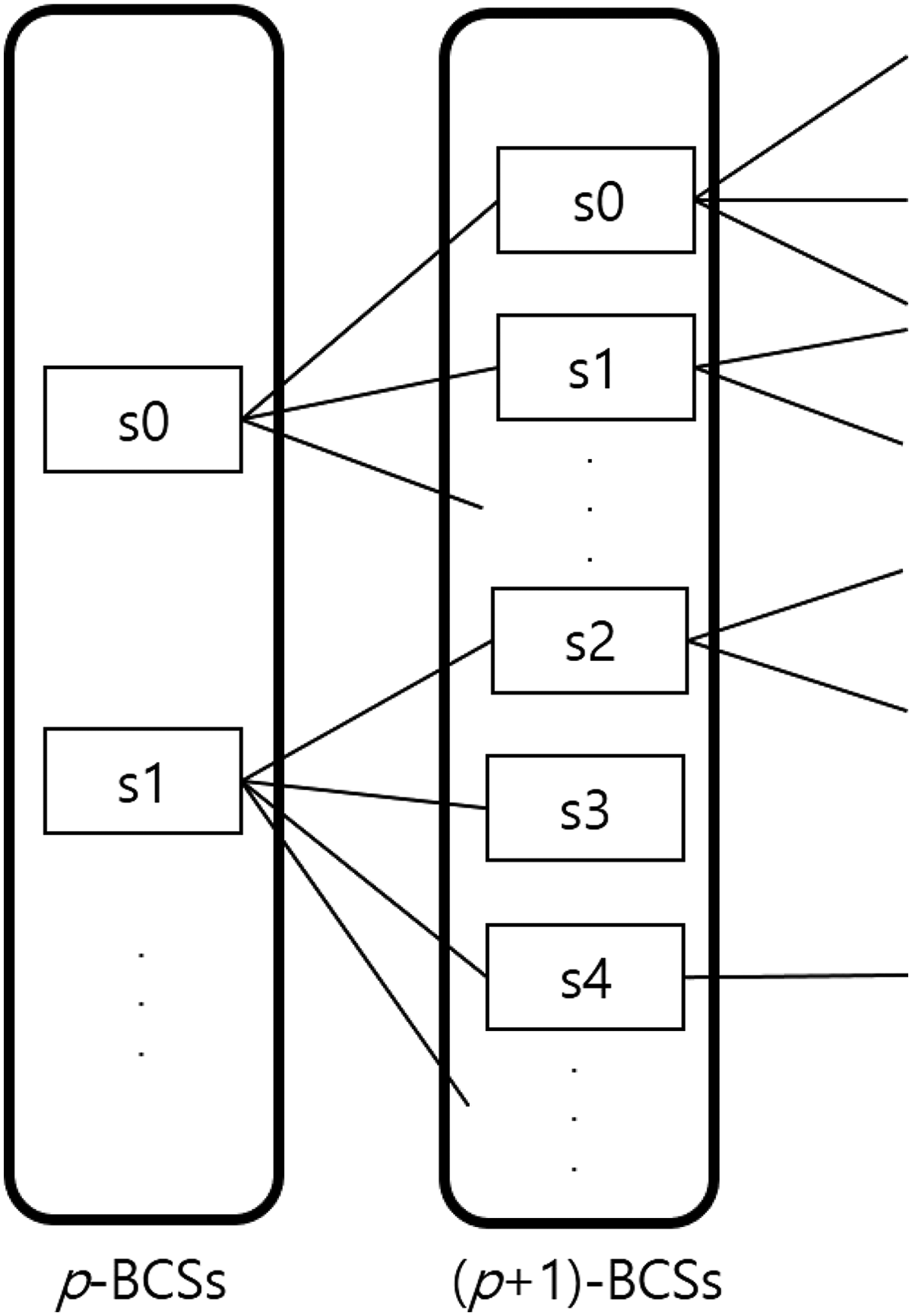
Obtaining (p + 1)-BCSs from p-BCSs using breadth-first search. p-BCS, bicluster candidate set consisting of p samples.

When a (p + 1)-BCS is obtained from a p-BCS, genes having similar patterns of expression values are grouped together to form the (p + 1)-BCS. The similarity between them is measured by the following \documentclass{aastex}\usepackage{amsbsy}\usepackage{amsfonts}\usepackage{amssymb}\usepackage{bm}\usepackage{mathrsfs}\usepackage{pifont}\usepackage{stmaryrd}\usepackage{textcomp}\usepackage{portland, xspace}\usepackage{amsmath, amsxtra}\usepackage{upgreek}\pagestyle{empty}\DeclareMathSizes{10}{9}{7}{6}\begin{document} $$\lambda$$ \end{document} value in the gene k: \documentclass{aastex}\usepackage{amsbsy}\usepackage{amsfonts}\usepackage{amssymb}\usepackage{bm}\usepackage{mathrsfs}\usepackage{pifont}\usepackage{stmaryrd}\usepackage{textcomp}\usepackage{portland, xspace}\usepackage{amsmath, amsxtra}\usepackage{upgreek}\pagestyle{empty}\DeclareMathSizes{10}{9}{7}{6}\begin{document} \begin{align*} \lambda _ { ij } ^k \;=\; \left\vert { { \frac { d_ { ij } ^k } { d_ { 01 } ^k } } } \right\vert. \tag { 3 } \end{align*} \end{document}

Here, \documentclass{aastex}\usepackage{amsbsy}\usepackage{amsfonts}\usepackage{amssymb}\usepackage{bm}\usepackage{mathrsfs}\usepackage{pifont}\usepackage{stmaryrd}\usepackage{textcomp}\usepackage{portland, xspace}\usepackage{amsmath, amsxtra}\usepackage{upgreek}\pagestyle{empty}\DeclareMathSizes{10}{9}{7}{6}\begin{document} $$d_{ij}^k$$ \end{document} is the expression value of the j^th sample in the sample set (p-BCS): the expression value of the i^th sample in the sample set (p-BCS) in the k^th gene. To combine genes having similar patterns, a gene set in which the \documentclass{aastex}\usepackage{amsbsy}\usepackage{amsfonts}\usepackage{amssymb}\usepackage{bm}\usepackage{mathrsfs}\usepackage{pifont}\usepackage{stmaryrd}\usepackage{textcomp}\usepackage{portland, xspace}\usepackage{amsmath, amsxtra}\usepackage{upgreek}\pagestyle{empty}\DeclareMathSizes{10}{9}{7}{6}\begin{document} $$\lambda$$ \end{document} value satisfies the following two conditions is searched when (p + 1)-BCS is expanded from p-BCS: (1) the sign of \documentclass{aastex}\usepackage{amsbsy}\usepackage{amsfonts}\usepackage{amssymb}\usepackage{bm}\usepackage{mathrsfs}\usepackage{pifont}\usepackage{stmaryrd}\usepackage{textcomp}\usepackage{portland, xspace}\usepackage{amsmath, amsxtra}\usepackage{upgreek}\pagestyle{empty}\DeclareMathSizes{10}{9}{7}{6}\begin{document} $$\lambda$$ \end{document} value is the same (2) max( \documentclass{aastex}\usepackage{amsbsy}\usepackage{amsfonts}\usepackage{amssymb}\usepackage{bm}\usepackage{mathrsfs}\usepackage{pifont}\usepackage{stmaryrd}\usepackage{textcomp}\usepackage{portland, xspace}\usepackage{amsmath, amsxtra}\usepackage{upgreek}\pagestyle{empty}\DeclareMathSizes{10}{9}{7}{6}\begin{document} $$\left\vert \lambda \right\vert$$ \end{document} ) ≤ min( \documentclass{aastex}\usepackage{amsbsy}\usepackage{amsfonts}\usepackage{amssymb}\usepackage{bm}\usepackage{mathrsfs}\usepackage{pifont}\usepackage{stmaryrd}\usepackage{textcomp}\usepackage{portland, xspace}\usepackage{amsmath, amsxtra}\usepackage{upgreek}\pagestyle{empty}\DeclareMathSizes{10}{9}{7}{6}\begin{document} $$\left\vert \lambda \right\vert$$ \end{document} ) × δ². Here, the δ value is a threshold value determined by the user, which is >1.

Specifically, we divide the \documentclass{aastex}\usepackage{amsbsy}\usepackage{amsfonts}\usepackage{amssymb}\usepackage{bm}\usepackage{mathrsfs}\usepackage{pifont}\usepackage{stmaryrd}\usepackage{textcomp}\usepackage{portland, xspace}\usepackage{amsmath, amsxtra}\usepackage{upgreek}\pagestyle{empty}\DeclareMathSizes{10}{9}{7}{6}\begin{document} $$\lambda$$ \end{document} value calculated from each gene by sign, and then sort the genes in ascending order. Then, the range is calculated by multiplying \documentclass{aastex}\usepackage{amsbsy}\usepackage{amsfonts}\usepackage{amssymb}\usepackage{bm}\usepackage{mathrsfs}\usepackage{pifont}\usepackage{stmaryrd}\usepackage{textcomp}\usepackage{portland, xspace}\usepackage{amsmath, amsxtra}\usepackage{upgreek}\pagestyle{empty}\DeclareMathSizes{10}{9}{7}{6}\begin{document} $$s_{ij}^k$$ \end{document} of the first gene by \documentclass{aastex}\usepackage{amsbsy}\usepackage{amsfonts}\usepackage{amssymb}\usepackage{bm}\usepackage{mathrsfs}\usepackage{pifont}\usepackage{stmaryrd}\usepackage{textcomp}\usepackage{portland, xspace}\usepackage{amsmath, amsxtra}\usepackage{upgreek}\pagestyle{empty}\DeclareMathSizes{10}{9}{7}{6}\begin{document} $${ \delta ^{1 / 8}}$$ \end{document} , and the genes having similar \documentclass{aastex}\usepackage{amsbsy}\usepackage{amsfonts}\usepackage{amssymb}\usepackage{bm}\usepackage{mathrsfs}\usepackage{pifont}\usepackage{stmaryrd}\usepackage{textcomp}\usepackage{portland, xspace}\usepackage{amsmath, amsxtra}\usepackage{upgreek}\pagestyle{empty}\DeclareMathSizes{10}{9}{7}{6}\begin{document} $$\lambda _{ij}^k$$ \end{document} values are grouped. All genes are grouped into small groups, and then 16 small groups are grouped into large groups to form the next candidate gene set. At this time, any set smaller than mg is discarded.

Figure 3 shows an example of this gene grouping process when δ is 2. First, we multiply the lowest \documentclass{aastex}\usepackage{amsbsy}\usepackage{amsfonts}\usepackage{amssymb}\usepackage{bm}\usepackage{mathrsfs}\usepackage{pifont}\usepackage{stmaryrd}\usepackage{textcomp}\usepackage{portland, xspace}\usepackage{amsmath, amsxtra}\usepackage{upgreek}\pagestyle{empty}\DeclareMathSizes{10}{9}{7}{6}\begin{document} $$\lambda$$ \end{document} value by \documentclass{aastex}\usepackage{amsbsy}\usepackage{amsfonts}\usepackage{amssymb}\usepackage{bm}\usepackage{mathrsfs}\usepackage{pifont}\usepackage{stmaryrd}\usepackage{textcomp}\usepackage{portland, xspace}\usepackage{amsmath, amsxtra}\usepackage{upgreek}\pagestyle{empty}\DeclareMathSizes{10}{9}{7}{6}\begin{document} $${ \delta ^{1 / 8}}$$ \end{document} to obtain a range and bind genes into a small group. In this example, the lowest \documentclass{aastex}\usepackage{amsbsy}\usepackage{amsfonts}\usepackage{amssymb}\usepackage{bm}\usepackage{mathrsfs}\usepackage{pifont}\usepackage{stmaryrd}\usepackage{textcomp}\usepackage{portland, xspace}\usepackage{amsmath, amsxtra}\usepackage{upgreek}\pagestyle{empty}\DeclareMathSizes{10}{9}{7}{6}\begin{document} $$\lambda$$ \end{document} value is 0.6. So, we multiply 0.6 by \documentclass{aastex}\usepackage{amsbsy}\usepackage{amsfonts}\usepackage{amssymb}\usepackage{bm}\usepackage{mathrsfs}\usepackage{pifont}\usepackage{stmaryrd}\usepackage{textcomp}\usepackage{portland, xspace}\usepackage{amsmath, amsxtra}\usepackage{upgreek}\pagestyle{empty}\DeclareMathSizes{10}{9}{7}{6}\begin{document} $${ \delta ^{1 / 8}}$$ \end{document} to find the range of the first group. The range of the first small group (i.e., small group 1) is then between 0.6 and 0.654. Similarly, the range of the second small group is between 0.6 × \documentclass{aastex}\usepackage{amsbsy}\usepackage{amsfonts}\usepackage{amssymb}\usepackage{bm}\usepackage{mathrsfs}\usepackage{pifont}\usepackage{stmaryrd}\usepackage{textcomp}\usepackage{portland, xspace}\usepackage{amsmath, amsxtra}\usepackage{upgreek}\pagestyle{empty}\DeclareMathSizes{10}{9}{7}{6}\begin{document} $${ \delta ^{1 / 8}}$$ \end{document} and 0.6 × \documentclass{aastex}\usepackage{amsbsy}\usepackage{amsfonts}\usepackage{amssymb}\usepackage{bm}\usepackage{mathrsfs}\usepackage{pifont}\usepackage{stmaryrd}\usepackage{textcomp}\usepackage{portland, xspace}\usepackage{amsmath, amsxtra}\usepackage{upgreek}\pagestyle{empty}\DeclareMathSizes{10}{9}{7}{6}\begin{document} $${ \delta ^{2 / 8}}$$ \end{document} , equivalent to between 0.654 and 0.713, so g₄ and g₂ belong to this small group (Fig. 3). We repeat this process until all the genes belong to the small group, and when the small group is completed, repeat the process to bind the 16 small groups into a large group (Fig. 3). In this example, large group 1 is composed of {g₁, g₄, g₂, g₁₁, g₅, …, g₃}. Note that the number of small groups is set to 16 since the preliminary experiments show that both finer (32 or 64) and coarser (4 or 8) bin sizes do not improve the quality of final output biclusters.

FIG. 3.

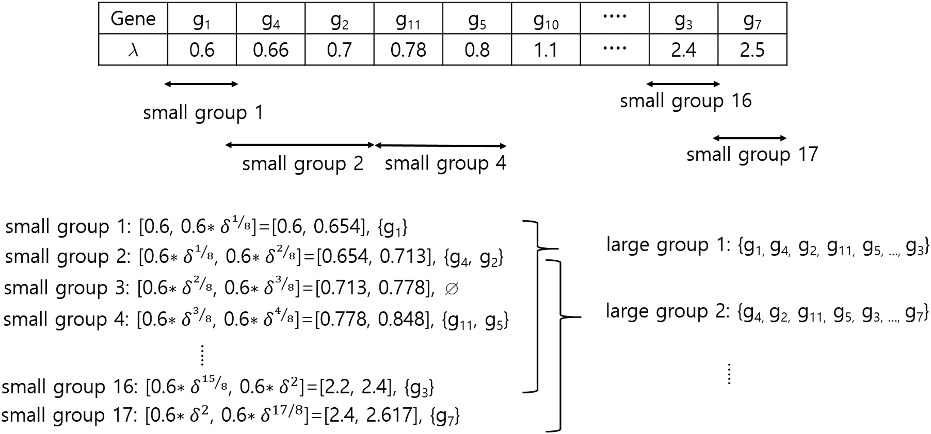
Example of gene grouping process when δ = 2.

3.2.4. Step 4: Queuing

When we expand (p + 1)-BCSs from p-BCSs, many duplicate gene sets may exist. Due to memory issues, we cannot keep all BCSs in memory. Priority queuing is used to solve this problem. We prioritize genes with large gene sets, since our goal is to find large biclusters with diverse memberships. Unlike Ahn et al. (2011), we used a single, rather than a multiple, priority queue, since preliminary experiments showed that a large number of gene sets in BCSs overlap in different queues. When multiple priority queuing is used as in Ahn et al. (2011), both small and large size gene sets may coexist in each queue. But due to these large gene sets, when duplicate BCSs are removed from each queue (step 4), the smaller size gene sets are removed first from the queue and as a result, only the duplicate gene sets remain in each queue. This approach eliminates the chance that small gene sets, which are removed from this queue, could expand to a more diverse set of genes. Therefore, we use a single priority queue and remove redundant large size gene sets through duplicate BCS removal process (step 4), with the result that diverse gene sets remain in the queue.

Figure 4 shows an example of why single priority queuing is preferable to multiple priority queuing. In this example, a similarity threshold between two BCSs specified by the user, (st), is set to 0.6. When multiple priority queues are used as shown in Figure 4a, the gene set {g₅, g₆, g₇} is removed from the first queue, because the overlapping ratio of the gene set, {g₅, g₆, g₇}, is 1, which is larger than the st value. But the gene set {g₁, g₂, g₃, g₄, g₅, g₆, g₇} will remain in priority queue 1. Similarly, in priority queue 2, the gene set {g₆, g₇, g₈, g₉, g₁₀} is removed because the overlapping ratio (i.e., 0.6) is equal to the st value. Therefore, the gene set {g₂, g₃, g₄, g₅, g₆, g₇, g₈} remains in priority queue 2. However, the two gene sets {g₁, g₂, g₃, g₄, g₅, g₆, g₇} and {g₂, g₃, g₄, g₅, g₆, g₇, g₈} remaining in each queue are very similar. If we use a single priority queue as shown in Figure 4b, one of the two gene sets, {g₁, g₂, g₃, g₄, g₅, g₆, g₇} and {g₂, g₃, g₄, g₅, g₆, g₇, g₈}, will be removed. Also, gene set {g₆, g₇, g₈, g₉, g₁₀} is not removed, since its overlap ratio, 0.4, is smaller than the st value (0.6).

FIG. 4.

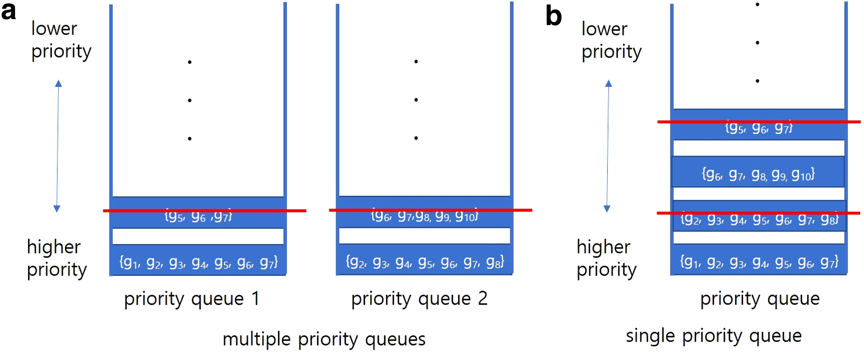
Comparison of two priority queuing strategies when st = 0.6. (a) Multiple priority queuing; (b) single priority queuing.

3.2.5. Step 5: Remove duplicate BCSs

In the priority queue, there exist many BCSs with duplicate gene sets. The process of removing the duplicate BCSs is as follows: first, the BCS with the highest priority (the BCS with the largest gene set) is compared with the rest of the BCSs in the priority queue. If the overlapping ratio of the two BCSs intersecting each other exceeds st, then the BCS with the smaller size is removed. Second, the BCS with the second highest priority among the remaining BCSs is compared with the rest of the BCSs, and if the overlapping ratio of the two BCSs intersecting each other exceeds st, then the BCS with the smaller size is removed. This process is repeated until the BCS with the lowest priority has been handled.

In Ahn et al. (2011), there is an additional step of removing duplicate BCSs using a bit string after performing the above duplicate BCS removal process. First, the algorithm finds the gene with the highest index among the remaining genes and creates a bit string of that size whose bits are all false (0). Then, from the highest priority gene set in the queue, we set the i^th bit of the bit string to true (t) if the i^th bit is false, and the gene set includes i^th gene. Let the ratio be \documentclass{aastex}\usepackage{amsbsy}\usepackage{amsfonts}\usepackage{amssymb}\usepackage{bm}\usepackage{mathrsfs}\usepackage{pifont}\usepackage{stmaryrd}\usepackage{textcomp}\usepackage{portland, xspace}\usepackage{amsmath, amsxtra}\usepackage{upgreek}\pagestyle{empty}\DeclareMathSizes{10}{9}{7}{6}\begin{document} $$ { \frac { { \rm { Number \;of \;genes \;that \;was \;newly \;set \;to \;true } } } { { \rm { Total \;number \;of \;genes \;in \;the \;gene \;set } } } } $$ \end{document} . If the ratio of a gene set is higher than st, that gene set is retained, and the algorithm proceeds to the next gene set. Otherwise, the gene set is removed, and the bits that were newly set to true return to false (Ahn et al., 2011).

In this work, we do not use this duplicate BCS removal process using a bit string, since it could remove a gene set that will expand to a unique bicluster. Figure 5 shows one example when st is 0.6. Suppose there are three gene sets, {g₁, g₂, g₃, g₄, g₅}, {g₈, g₉, g₁₀, g₁₁, g₁₂}, and {g₅, g₆, g₇, g₈}, in the priority queue. Then, when the duplicate BCS removal process using the bit string is used, gene set {g₁, g₂, g₃, g₄, g₅} and gene set {g₈, g₉, g₁₀, g₁₁, g₁₂} corresponding bits are changed to 1 in the bit string and retained (Fig. 5). And the gene set, {g₅, g₆, g₇, g₈}, is removed, because its ratio is 2/4, which is smaller than the st value (0.6). However, the removed gene set, {g₅, g₆, g₇, g₈}, overlaps only a small portion of other two gene sets.

FIG. 5.

Elimination of duplicate BCSs when st = 0.6.

4. Results

4.1. Datasets

To evaluate the effectiveness of the RN⁺ algorithm, a total of five real microarray datasets, GDS181, GDS589, GDS1027, GDS1406, and GDS1490, were used (Padilha et al., 2017). The datasets include Homo sapiens, Rattus norvegicus, and Mus musculus (Table 1). We also downloaded PPI network data from BioGRID (Oughtred et al., 2019) for H. sapiens, R. norvegicus, and M. musculus. The detailed information is shown in Table 2.

Table 1.

Description of Gene Expression Datasets

Dataset	No. of genes	No. of samples	Description	Species
GDS181	12,094	84	Human and mouse	Homo sapiens
GDS589	7747	122	Multiple normal tissue gene expression across strains	Rattus norvegicus
GDS1027	12,452	154	Sulfur mustard effect on lungs	R. norvegicus
GDS1406	12,488	87	Brain regions of various inbred strains	Mus musculus
GDS1490	11,926	150	Neural tissue profiling	M. musculus

Table 2.

Description of Protein–Protein Interaction Datasets

Species	No. of genes (proteins)	No. of interactions
H. sapiens	16,746	439,366
R. norvegicus	2796	6326
M. musculus	7656	44,995

4.2. Parameters

The following parameters were used: the deg_th is used to identify high-degree genes and is set to 0.01. The dist_th is set to 2. The edge_th is set to 0.001. The minimum number of samples in the BCS specified by the user, mns, is set to 4. The mng is the minimum number of genes and is set to 30. The st value represents degree of overlap between biclusters. We set st = 0.7. When the st value increases, more biclusters can be found since the parameter allows bicluster overlaps with other biclusters. Queue size was set to 1000. The δ value is a user-specified parameter that determines how much of the t-value difference in the same BCS should be tolerated. The δ value is set to 1.8 to find as many diverse biclusters as possible.

4.3. Computational cost of RN⁺

Let the number of genes and samples in microarray data be m and n, respectively. The computational cost of the first step, which finds 2-BCSs, is O(n²) since there are C(n,2) sample pairs. The second step is to find (p + 1)-BCSs from p-BCSs. For each BCS, at most n samples need to be examined and there are at most m groups during the gene grouping process. Also, we need to sort the genes with respect to s values. Thus, it takes O(nmlogm) when quick sort is used. Obtaining all (p + 1)-BCSs from all p-BCS occurs at most n times. Therefore, in total the RN⁺ algorithm approximately takes O(n²mlogm).

We implemented the RN⁺ biclustering algorithm using C++. We calculated the running time of RN⁺ by varying the number of rows (genes) while fixing the number of columns (samples) as 50. The RN⁺ algorithm is tested on a computer with 3.2 GHz quad-core Intel i5-6500 CPUs and 8 GB main memory. Figure 6 shows the running time of the RN⁺ algorithm with respect to the number of rows. We observe an almost linear relationship as the number of genes increases.

FIG. 6.

Running time of the RN⁺ with increasing number of genes when the number of columns (samples) is 50.

4.4. Comparison

A total of seven state-of-the-art biclustering algorithms were compared for the experiments: RN clustering (Ahn et al., 2011), Cheng and Church (CC) (Cheng and Church, 2000), ISA (Bergmann et al., 2003), OPSM (Ben-Dor et al., 2003), Plaid (Lazzeroni and Owen, 2000), QUBIC (Li et al., 2009), SAMBA (Tanay et al., 2002), and UniBIC (Wang et al., 2016). The author of the RN clustering algorithm provided the source code (Ahn et al., 2011), which was implemented in C++ (Table 3).

Table 3.

Biclustering Algorithms and Implementations Used in Our Experiments

Algorithm	Implementation	Available at
CC	R	https://cran.r-project.org/web/packages/biclust/biclust.pdf
ISA	R	https://cran.r-project.org/web/packages/isa2/index.html
OPSM	JAVA	https://sop.tik.ee.ethz.ch/bicat
Plaid	R	https://cran.r-project.org/web/packages/biclust/biclust.pdf
QUBIC	R	https://bioconductor.org/packages/release/bioc/html/QUBIC.html
UniBIC	R	https://bioconductor.org/packages/devel/bioc/vignettes/runibic/inst/doc/runibic.html

CC, Cheng and Church; ISA, iterative signature algorithm; OPSM, Order-Preserving Submatrix; QUBIC, Qualitative Biclustering; UniBIC, sequential row-based biclustering algorithm for analysis of gene expression data.

4.5. GO evaluation

The number of biclusters found and enriched after filtering out the highly overlapped biclusters for each algorithm at a significance level of 5% is shown in Table 4. Biclusters are considered to be enriched if any GO term was smaller than p = 0.05 (Eren et al., 2012). The RN⁺ algorithm finds the largest number of biclusters compared with the other state-of-the-art biclustering algorithms we explored. The RN⁺ algorithm found 552 enriched biclusters from 561 discovered. It outperformed the RN algorithm in terms of both the enriched biclusters and the percentage of biclusters found. The ISA algorithm achieved 100% enriched proportion but found only 30 biclusters on five real datasets. The CC algorithm found 493 biclusters, but most of them are not biologically meaningful. Similarly, UniBIC found 495 biclusters, but only 68.2% of them are enriched. Figure 7 shows the proportions of the enriched biclusters for each algorithm at five different significance levels. The results of five real datasets are aggregated. We observed that the RN⁺ algorithm outperformed the RN algorithm at all significance levels. The ISA algorithm showed 100% proportion but only found 30 biclusters at all significance levels.

FIG. 7.

Proportion of the enriched biclusters for various biclustering algorithms on five different significance levels (p). CC, Cheng and Church; ISA, iterative signature algorithm; OPSM, Order-Preserving Submatrix; QUBIC, Qualitative Biclustering; UniBIC, sequential row-based biclustering algorithm for analysis of gene expression data.

Table 4.

Accumulated Number of Biclusters and Enriched Biclusters on Five Real Datasets at a Significance Level of 5%

Algorithm	Found	Enriched (%)
RN⁺	561	552 (98.3)
RN	232	217 (93.5)
OPSM	27	22 (81.4)
ISA	30	30 (100.0)
Plaid	33	29 (87.8)
QUBIC	58	55 (94.8)
CC	493	126 (25.5)
UniBIC	495	338 (68.2)

5. Conclusion

In this article, we have proposed a novel biclustering method, RN⁺, for finding biologically meaningful biclusters in microarray data. The RN⁺ algorithm identified biologically significant biclusters by performing a unique gene filtering, gene searching, gene grouping, and queuing process, using PPI network data. Unlike previous approaches, the RN⁺ method performs biclustering only for highly related genes in the PPI network using the gene filtering process. It also uses a single priority queuing scheme to effectively construct a breadth-first tree, and removes redundant BCSs to identify diverse biclusters. We compared the RN⁺ algorithm with several competitive biclustering algorithms on five real datasets. The GO database was used to validate the biological significance. Experimental results show that RN⁺ was able to find a significantly larger number of functionally enriched and biologically meaningful biclusters compared with those of competitive biclustering algorithms.

Footnotes

Acknowledgment

This research was supported by the Incheon National University Research Grant in 2018.

Author Disclosure Statement

The authors declare that no competing financial interests exist.

References

Ahn

, Yoon

, and Park

2011. Noise-robust algorithm for identifying functionally associated biclusters from gene expression data. Inform. Sci. 181, 435–449.

Ben-Dor

, Chor

, Karp

, et al. 2003. Discovering local structure in gene expression data: The order-preserving submatrix problem. J. Comput. Biol. 10, 373–384.

Bergmann

, Ihmels

, and Barkai

2003. Iterative signature algorithm for the analysis of large-scale gene expression data. Phy. Rev. E, 67, 031902.

Bhattacharya

, and Cui

2017. A GPU-accelerated algorithm for biclustering analysis and detection of condition-dependent coexpression network modules. Sci. Rep. 7, 4162.

Cheng

, and Church

2000. Biclustering of expression data, 93–103. Presented at Proc. ISMB'00. AAAI Press, Menlo Park, CA.

Eren

, Deveci

, Küçüktunç

, et al. 2012. A comparative analysis of biclustering algorithms for gene expression data. Brief Bioinform. 14, 279–292.

Lazzeroni

, and Owen

2000. Plaid models for gene expression data. Technical Report. Stanford University.

, Ma

, Tang

, et al. 2009. QUBIC: A qualitative biclustering algorithm for analyses of gene expression data. Nucleic Acids Res. 37, e101.

, Guo

, Wu

, et al. 2012. A comparison and evaluation of five biclustering algorithms by quantifying goodness of biclusters for gene expression data. BioData Min. 5, 8.

10.

Oughtred

, Start

, Breitkreutz

B.-J.

, et al. 2019. The BioGRID interaction database: 2019 update. Nucleic Acids Res. 47, D529–D541.

11.

Padilha

V.A.

, and Campello

R.J.G.B.

2017. A systematic comparative evaluation of biclustering techniques. BMC Bioinformatics, 18, 55.

12.

Saullo

, Veroneze

, Zuben

F.J.V.

, et al. 2015. On bicluster aggregation and its benefits for enumerative solutions. Presented at the International Workshop on Machine Learning and Data Mining in Pattern Recognition. Springer, Cham.

13.

Tanay

, Sharan

, and Shamir

2002. Discovering statistically significant biclusters in gene expression data. Bioinformatics, 18 Suppl 1, S136–S144.

14.

Wang

, Li

, Robinson

R.W.

, et al. 2016. UniBic: Sequential row-based biclustering algorithm for analysis of gene expression data. Sci. Rep. 6, 23466.

15.

, Lu

, Tung

, et al. 2006. Mining shifting-and-scaling co-regulation patterns on gene expression profiles. Presented at ICDE'06, 89, Atlanta, GA.

16.

Yun

, and Yi

G.S.

2013. Biclustering for the comprehensive search of correlated gene expression patterns using clustered seed expansion. BMC Genomics, 14, 144.

RN + : A Novel Biclustering Algorithm for Analysis of Gene Expression Data Using Protein–Protein Interaction Network

Abstract

Abstract

1. Introduction

2. Related Work

3. Method

3.1. Notations

3.2. RN+ algorithm

3.2.1. Step 1: Gene filtering using gene network data

3.2.2. Step 2: Find 2-BCS

3.2.3. Step 3: Obtain (p + 1)-BCSs from p-BCSs

3.2.4. Step 4: Queuing

3.2.5. Step 5: Remove duplicate BCSs

4. Results

4.1. Datasets

4.2. Parameters

4.3. Computational cost of RN+

4.4. Comparison

4.5. GO evaluation

5. Conclusion

Footnotes

Acknowledgment

Author Disclosure Statement

References

3.2. RN⁺ algorithm

4.3. Computational cost of RN⁺