Predicting the Number of Bases to Attain Sufficient Coverage in High-Throughput Sequencing Experiments

Abstract

For many types of high-throughput sequencing experiments, success in downstream analysis depends on attaining sufficient coverage for individual positions in the genome. For example, when identifying single-nucleotide variants de novo, the number of reads supporting a particular variant call determines our confidence in that variant call. If sequenced reads are distributed uniformly along the genome, the coverage of a nucleotide position is easily approximated by a Poisson distribution, with rate equal to average sequencing depth. Unfortunately, as has become well known, high-throughput sequencing data are never uniform. The numerous factors contributing to variation in coverage have resisted attempts at direct modeling and change along with minor adjustments in the underlying technology. We propose a new nonparametric method to predict the portion of a genome that will attain some specified minimum coverage, as a function of sequencing effort, using information from a shallow sequencing experiment from the same library. Simulations show our approach performs well under an array of distributional assumptions that deviate from uniformity. We applied this approach to estimate coverage at varying depths in single-cell whole-genome sequencing data from multiple protocols. These resulted in highly accurate predictions, demonstrating the effectiveness of our approach in analyzing complexity of sequencing libraries and optimizing design of sequencing experiments.

1. Introduction

Genome coverage is a critical technical characteristic of high-throughput genomic sequencing experiments (Sims et al., 2014). High coverage is necessary for correcting sequencing errors and for credible biological conclusions. For example, in single-nucleotide variant detection, candidate variants supported by few reads are often filtered out to reduce false positives caused by sequencing errors (Chen et al., 2017; Xu, 2018). However, the cost of sequencing is proportional to the total amount of nucleotides sequenced. To plan sequencing experiments and determine the appropriate allotment of sequencing effort in a given experiment, experimental design must consider the portion of sites in the genome expected to attain sufficient coverage as a function of total nucleotides sequenced. To indicate “sufficient” coverage, we define a site as having sufficient coverage if the site is covered by at least r reads. Here the value r is predetermined by the experiment's designer, based on goals and subsequent analyses. For example, a value of r = 8 has been used to select high-confident single-nucleotide polymorphism candidates as those supported by at least eight reads (Ng et al., 2010). Similarly, a value of r = 5 has been used in identification of indels (The 1000 Genomes Project Consortium, 2012) and a value of r = 3 has been used in detection of ultrarare de novo mutations (Eboreime et al., 2016). For a specified value of r, we seek to estimate the number of sites covered by at least r reads as a function of the sequencing effort.

Excessive variance of coverage along the genome in high-throughput sequencing can be attributed, in large part, to sequence-specific factors. First, DNA fragments in sequencing libraries amplify with different efficiencies. GC-rich and AT-rich DNA fragments have been found underrepresented in sequencing results (Benjamini and Speed, 2012). Second, parts of genomes can go missing during sequencing library preparation. In particular, for single-cell whole-genome sequencing (scWGS), this dropout rate is high compared with bulk sequencing experiments due to the low amount of DNA in a single cell. Given an equal number of sequenced reads, different scWGS experiments can exhibit quite different coverage profiles (Chen et al., 2017). This high and unpredictable variance presents difficulties in formulating any general guidelines for how many total reads to sequence in a given experiment.

The pioneering work in this area is the well-known Lander/Waterman theory (Lander and Waterman, 1988), which relates genome coverage to sequencing effort for Sanger sequencing (Sanger et al., 1977). The basic statistical assumption of the Lander/Waterman model is that reads are generated uniformly at random from the genome. Under this assumption, for each site in the genome, the number of reads that cover this site can be approximated by a Poisson distribution, where the Poisson rate λ is estimated by average sequencing depth using maximum likelihood estimation. The Lander/Waterman theory fits extremely well for Sanger sequencing, and it elegantly accounts for many intricacies relevant to de novo sequence assembly. Although many of the statistical questions we face in high-throughput sequencing applications appear more straightforward, this theory is largely inapplicable when faced with highly variable sequencing coverage (Benjamini and Speed, 2012; Daley and Smith, 2013).

Instead of using the same Poisson rate λ for each site, in this article, we assume that the Poisson rate λ varies among sites and follows a latent distribution G(λ), which is used to describe all varieties of coverage along the genome. Mixtures of Poisson distributions have seen wide use for inferences on the relationship between species and individuals (Engen, 1978). To connect the terminology from this body of literature with our application, one can regard species as sites in a genome, and sequenced nucleotides mapping over those base-pairs are the sampled individuals. As a notable early example, Fisher et al. (1943) assumed that the latent G(λ) is a gamma distribution. Although other parametric distributions have been investigated (Bhattacharya, 1966; Bulmer, 1974; Sichel, 1975; Burrell and Fenton, 1993), it is hard to assess which parametric distribution should be applied based on observed data. In particular, distinct parametric forms may appear to fit observed data well, but exhibit very different extrapolation behaviors (Engen, 1978). In this context, extrapolation means predicting the number of species in a sample of larger size—expanding the number of observed individuals.

Good and Toulmin (1956) established a nonparametric empirical Bayes framework that served as the foundation for much subsequent nonparametric methodology (Efron and Thisted, 1976; Boneh et al., 1998; Chao and Shen, 2004; Daley and Smith, 2013). For the case r = 1, Good and Toulmin (1956) derived an estimator for the expected number of species in a sample while avoiding direct inference of G(λ). This estimator takes the form of an alternating power series, which is accurate for short-range extrapolation but diverges in practice for long-range extrapolation (Good and Toulmin, 1956). Daley and Smith (2013) proposed a solution to the divergence problem by applying rational function approximation to the Good/Toulmin power series. This approach showed promising results in predicting library complexity (Daley and Smith, 2013), the number of sites covered by at least one read (Daley and Smith, 2014), and other applications (Deng et al., 2015). However, because this method does not infer the latent distribution, it did not suggest an extension to predict the number of sites covered by at least r > 1 reads as a function of sequencing effort (Daley, 2014).

Intuitively, predicting genome coverage seems more difficult when r > 1 compared with r = 1. In the example of Figure 1a, the curve for the number of sites covered by at least r = 1 read appears flat after 500 reads, suggesting that the sample is saturated. However, barely any sites are covered at least r = 16 times after sequencing 500 reads—leading to a very different flat curve. Visually inspecting the shape of the curve for r = 16 based on 500 reads (Fig. 1a) provides very little information about the shape of the curve after 3000 reads (Fig. 1b).

FIG. 1.

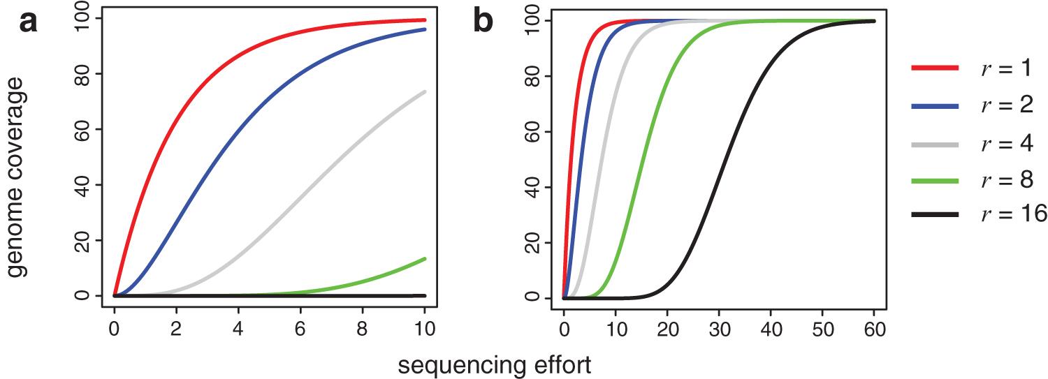
The expected number of sites in the genome covered by at least r reads as a function of the sequencing effort. In this toy example, we assume that the length of the reference genome is 100 bp. One unit in the x-axis represents 50 reads with read length 1. The number of reads is up to (a) 500 (10 U) and (b) 3000 (60 U).

We propose a new method to predict the expected number of sites in the genome covered by at least r reads as a function of the sequencing effort. To overcome the difficulties of generalizing nonparametric methods from r = 1 to r > 1, we first derive a relationship between the expected number of sites covered by at least r reads and the expected number of sites covered by at least one read, under the mixture of Poisson distribution assumption. Without inferring the latent distribution, this derived relationship can generalize any smooth expression, which is used to calculate the expected number of sites covered by at least r = 1 read as a function of the sequencing effort, to an expression for r > 1. We then utilize this relationship to construct a nonparametric estimator that can be applied for every value of r. We prove that our estimator converges as the sequencing effort goes to infinity, essential for large-scale applications such as high-throughput sequencing. Extensive simulations suggest that our estimator performs very well for various types of heterogeneous populations. Applications to scWGS data demonstrate accuracy as a basis for resource allocation in high-throughput sequencing experiments.

2. Unified Representation for Multiplicity of Coverage

We will use the conventional “species” terminology of Good (1953). The problem is as follows: a random sample of individuals is captured from a population after trapping for one unit of time. Each individual belongs to exactly one species, and the total number L of species in the population is finite but not known. In the context of sequencing, although the length of the reference genome is known, the actual observable/captured genome varies among prepared sequencing libraries. Let N_j be the number of species represented by exactly j individuals in this sample. Clearly N₀ is not observable. Imagine that a second sample is obtained after trapping for t units of time from the same population. The time t > 1 should bring to mind a “scaled up” experiment. This second sample may take the form of an expansion of the initial sample, but may also be a separate sampling experiment. Let S_r(t) be the random variable whose value is the number of species represented at least r times after trapping for t units of time. We are concerned with predicting the expected number $E [S_{r} (t)]$ . When plotted as a function of t, the quantity $E [S_{1} (t)]$ is known as the species accumulation curve (SAC). Similarly, as a function of t, we call $E [S_{r} (t)]$ the r-SAC (r-SAC).

For a given species, we assume that the number of individuals in a sample follows a Poisson distribution with expectation λ per unit time. To describe the heterogeneity of abundance among species, we assume the rate λ is generated from a latent distribution G(λ). Let N_j(t) be the random variable whose value is the number of species represented exactly j times after trapping for t units of time. By definition $E [S_{r} (t)] = \sum_{j = r}^{\infty} E [N_{j} (t)] = E [S_{1} (t)] - \sum_{j = 1}^{r - 1} E [N_{j} (t)] .$ (1)

From our Poisson mixture assumption, the expected number of species after trapping for t units of time can be expressed as follows: $E [S_{1} (t)] = L \int (1 - exp (- λ t)) d G (λ) .$

Taking the jth derivative of $E [S_{1} (t)]$ , we have

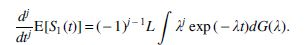
Note that the expected value of N_j(t) is as follows: $E [N_{j} (t)] = L \int \frac{{(λ t)}^{j} exp (- λ t)}{j!} d G (λ) = \frac{t^{j}}{j!} L \int λ^{j} exp (- λ t) d G (λ) .$

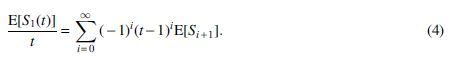
By comparing the above expression with the jth derivative of $E [S_{1} (t)]$ , we obtain the following: $E [N_{j} (t)] = \frac{{(- 1)}^{j - 1} t^{j}}{j!} \frac{d^{j}}{d t^{j}} E [S_{1} (t)],$ (2)

which has been noted previously (Kalinin, 1965). By replacing the $E [N_{j} (t)]$ in Equation (1) with the jth derivative of $E [S_{1} (t)]$ from Equation (2), we obtain a relationship between $E [S_{1} (t)]$ and $E [S_{r} (t)]$ . This is the foundation of our estimator, and a proof is found in the Supplementary Materials (Section S1.1).

Theorem 1. For any positive integer r, $E [S_{r} (t)] = \frac{{(- 1)}^{r - 1} t^{r}}{(r - 1)!} \frac{d^{r - 1}}{d t^{r - 1}} (\frac{E [S_{1} (t)]}{t}) .$ (3)

Thus, we have established a direct relationship between the SAC and the r-SAC. Using Equation (3), we can generalize any smooth expression for the SAC to the expression for the corresponding r-SAC. We demonstrate the use of Equation (3) by deriving the expression of the r-SAC for a few widely used methods that are designed for the SAC (Supplementary Materials in Section S2). We call the ratio $E [S_{1} (t)] ∕ t$ the average discovery rate, as it reflects the average rate at which new species are discovered. In Section 3, we apply Theorem 1 to construct a nonparametric estimator for the r-SAC.

3. A New Nonparametric Estimator

Here we leverage the technique of Padé approximation to build a nonparametric estimator for the r-SAC. A Padé approximant is a rational function with a Taylor expansion that agrees with the power series of the function it approximates up to a specified degree (Baker and Graves-Morris, 1996). In this sense, Padé approximants are rational functions that optimally approximate a power series. This method was successfully applied to construct the estimator of the SAC, using Padé approximants to the Good/Toulmin power series (Deng et al., 2015). Padé approximants are effective because they converge in practice when the Good/Toulmin power series does not, yet within the applicable range of Good/Toulmin power series (t < 2), the two functions remain close. We apply a similar idea beginning with the average discovery rate. This leads to an expression that simplifies the formula in Theorem 1, yielding a new and practical nonparametric estimator for the r-SAC.

Our first step is to obtain a power series representation for the average discovery rate $E [S_{1} (t)] ∕ t$ in terms of S_i, which is the number of species represented at least i times in the initial sample. A proof of the following result is found in the Supplementary Materials (Section S1.2).

Lemma 1. If 0 < t < 2, then

Replacing expectations with the corresponding observations, each of which is an unbiased estimator, we obtain an unbiased power series estimator of the average discovery rate:

This power series estimator ϕ(t) serves as a bridge between the observed data S_i and the Padé approximant for $E [S_{1} (t)] ∕ t$ , which cannot be obtained directly. The Padé approximant for $E [S_{1} (t)] ∕ t$ is defined by its behavior around t = 1, which is the region where $E [S_{1} (t)] ∕ t$ is close to ϕ(t). Note that, in principle, we could directly substitute the estimated power series ϕ(t) for the average discovery rate to obtain an unbiased power series estimator for $E [S_{r} (t)]$ . Unfortunately, this estimator practically diverges for t > 2, due to the small radius of convergence of the power series and the use of the truncated power series to approximate it (see Discussion in Supplementary Materials [Section S4]).

Although Padé approximants to a given function can have any combination of degrees for the numerator and denominator polynomials, we consider only the subset for which the difference in degree of the numerator and denominator is 1. Importantly, this choice permits these rational functions to mimic the long-term behavior of the average discovery rate, which should approach L/t for large t.

Let P_m_-1(t)/Q_m(t) denote the Padé approximant to power series ϕ(t) with numerator degree m − 1 and denominator degree m. According to the formal determinant representation (Baker and Graves-Morris, 1996), $\begin{matrix} \frac{P_{m - 1} (t)}{Q_{m} (t)} = \frac{a_{0} + a_{1} (t - 1) + \dots + a_{m - 1} {(t - 1)}^{m - 1}}{b_{0} + b_{1} (t - 1) + \dots + b_{m} {(t - 1)}^{m}} = \\ \frac{|\begin{matrix} {(- 1)}^{0} S_{1} & {(- 1)}^{1} S_{2} & \dots & {(- 1)}^{m - 1} S_{m} & {(- 1)}^{m} S_{m + 1} \\ {(- 1)}^{1} S_{2} & {(- 1)}^{2} S_{3} & \dots & {(- 1)}^{m} S_{m + 1} & {(- 1)}^{m + 1} S_{m + 2} \\ ⋮ & ⋮ & ⋱ & ⋮ & ⋮ \\ {(- 1)}^{m - 1} S_{m} & {(- 1)}^{m} S_{m + 1} & \dots & {(- 1)}^{2 m - 2} S_{2 m - 1} & {(- 1)}^{2 m - 1} S_{2 m} \\ 0 & {(- 1)}^{0} S_{1} {(t - 1)}^{m - 1} & \dots & \sum_{i = 0}^{m - 2} {(- 1)}^{i} S_{i + 1} {(t - 1)}^{i + 1} & \sum_{i = 0}^{m - 1} {(- 1)}^{i} S_{i + 1} {(t - 1)}^{i} \end{matrix}|}{|\begin{matrix} {(- 1)}^{0} S_{1} & {(- 1)}^{1} S_{2} & \dots & {(- 1)}^{m - 1} S_{m} & {(- 1)}^{m} S_{m + 1} \\ {(- 1)}^{1} S_{2} & {(- 1)}^{2} S_{3} & \dots & {(- 1)}^{m} S_{m + 1} & {(- 1)}^{m + 1} S_{m + 2} \\ ⋮ & ⋮ & ⋱ & ⋮ & ⋮ \\ {(- 1)}^{m - 1} S_{m} & {(- 1)}^{m} S_{m + 1} & \dots & {(- 1)}^{2 m - 2} S_{2 m - 1} & {(- 1)}^{2 m - 1} S_{2 m} \\ {(t - 1)}^{m} & {(t - 1)}^{m - 1} & \dots & (t - 1) & 1 \end{matrix}|} \end{matrix}$ (6)

The above representation allows us to reason algebraically about the existence of the desired Padé approximant to ϕ(t) for a given initial sample. Define the Hankel determinants as follows: $Δ_{i, j} = {|\begin{matrix} S_{i - j + 2} & S_{i - j + 3} & \dots & S_{i + 1} \\ S_{i - j + 3} & S_{i - j + 4} & \dots & S_{i + 2} \\ ⋮ & ⋮ & ⋱ & ⋮ \\ S_{i + 1} & S_{i + 2} & \dots & S_{i + j} \end{matrix}|}_{j \times j},$ (7)

with S_k = 0 for k < 1. A proof of the next lemma is given in the Supplementary Materials (Section S1.2).

Lemma 2. If the determinants Δ_m−1,m and Δ_m,m are nonzero, there exist real numbers a_i and b_j for i = 0,1,…,m − 1, and j = 1, 2,…,m, with b_m≠0, such that the rational function $\frac{P_{m - 1} (t)}{Q_{m} (t)} = \frac{a_{0} + a_{1} (t - 1) + \dots + a_{m - 1} {(t - 1)}^{m - 1}}{1 + b_{1} (t - 1) + \dots + b_{m} {(t - 1)}^{m}},$

satisfies $ϕ (t) - \frac{P_{m - 1} (t)}{Q_{m} (t)} = O ({(t - 1)}^{2 m}),$ (8)

and all a_i and b_j are uniquely determined by S ₁ ,S ₂ ,…,S _2m .

Combining Lemma 1 and 2, we constructed a nonparametric estimator Ψ_r,m(t) for the r-SAC in Theorem 2. The proof is found in the Supplementary Materials (Section S1.2). In what follows, we assume that denominators of all rational functions of interest have simple roots. Although in practice we do not encounter Q_m(t) with repeated roots, in the Supplementary Materials we show how this assumption can be removed.

Theorem 2. Let m be a positive integer. If both determinants Δ_m−1,m and Δ_m,m are nonzero, then there exist complex numbers c_i and x_i, uniquely determined by S₁, …, S_2m, such that for all 1 ≤ r ≤ 2m, $Ψ_{r, m} (t) = \sum_{i = 1}^{m} c_{i} {(\frac{t}{t - x_{i}})}^{r}$ (9)

satisfies Ψ_r,m(1) = S_r.

Of note, the coefficients c_i and poles x_i are independent of r: once determined, they can be used to directly evaluate Ψ_r,m(t) for any r. The estimator Ψ_r,m(t) has some favorable properties, summarized in the following proposition, with proofs given in the Supplementary Materials (Section S1.2).

Proposition 1. (i) The estimator Ψ_r,m(t) is unbiased for $E [S_{r} (t)]$ at t = 1 for r ≤ 2m.

(ii) The estimator Ψ_r,m(t) converges as t approaches infinity. In particular, ${lim}_{t \to \infty} Ψ_{r, m} (t) = \frac{Δ_{m - 1, m + 1}}{Δ_{m, m}} .$

(iii) The estimator Ψ_r,m(t) is strongly consistent as the initial sample size goes to infinity.

Remark. Both determinants Δ_m−1,m and Δ_m,m become 0 when S_j = L for j ≤ 2m and m > 1, so the determinant representation of the Padé approximant [Equation (6)] is ill-defined in such cases. However, the Padé approximant itself remains valid and reduces to L/t for t > 0 (Supplementary Materials in Section S1.3).

4. An Algorithm for Estimator Construction

4.1. Conditions for well-behaved rational functions

The choice of m controls the degree of both the numerator and the denominator in the Padé approximant, and determines the amount of information from the initial sample that is used by Ψ_r,m(t). In principle, m should be selected sufficiently large so that the estimator Ψ_r,m(t) can explain the complexity of the latent distribution G(λ). However, a larger value of m leads to more poles in the estimator Ψ_r,m(t) and makes instability more likely. In practice, the stability of the estimators depends on the locations of poles. For example, if any pole x_i resides on the positive real axis, then Ψ_r,m(t) is unbounded in the neighborhood of x_i and becomes ill-defined at t = x_i. Here we give a sufficient condition to stabilize the estimator so that it is well-defined and bounded for t ≥ 0 and r ≥ 1. Note: Re(x) is the real part of x. A proof of the next proposition is given in the Supplementary Materials (Section S1.4).

Proposition 2. If Re(x_i) < 0 for 1 ≤ i ≤ m, then Ψ_r,m(t) is bounded for any t ≥ 0 and r ≥ 1. Further, Ψ_r,m(t) → 0 as r → ∞ for any 0 ≤ t < ∞.

Remark. It is not unusual to constrain roots in such a way to ensure stability. For example, the Hurwitz polynomial, which has all zeros located in the left half-plane of the complex plane, is used as a defining criterion for a system of differential equations to have stable solutions (Rahman and Schmeisser, 2002).

Algorithm 1 Given a set of observed counts {N_j}, with N₁, N₂ > 0, and a value $m_{m a x}$ , produce the stable and increasing estimator Ψ_r,m(t) for maximal $m \leq m_{m a x}$ .
1: Compute sums $S_{i} = \sum_{j \geq i} N_{j}$ , for $i = 1, \dots, 2 m_{m a x}$ . These coefficients define ϕ(t).
2: Compute the coefficients of the degree $2 m_{m a x}$ continued fraction approximation to ϕ(t) by applying the quotient-difference algorithm.
3: for $m \leftarrow m_{m a x}$ to 1 do
4: Obtain the Padé approximant P_m_-1(t)/Q_m(t) by evaluating the 2m-th convergent of the continued fraction.
5: Obtain the roots x_i, for i = 1,…,m, of the denominator Q_m(t).
6: Calculate coefficients c_i by partial fraction decomposition of P_m_-1(t)/Q_m(t).
7: if Re(x_i) < 0 for all x_i and Ψ_1,m(t) is increasing then
8: return coefficients (c₁,…,c_m) and roots (x₁,…,x_m).

4.2. The construction algorithm

Algorithm 1 provides a complete procedure for constructing our estimator beginning with the observed counts N_j, and satisfying the conditions outlined above. This procedure requires specifying a maximum value of m, and also leaves room for using more effective numerical procedures at each step. Details about these procedures are found in the Supplementary Materials (Section S3).

To see that Algorithm 1 terminates successfully, note that when m = 1, $Ψ_{r, 1} (t) = \frac{S_{1}^{2}}{S_{2}} {(\frac{t}{t + (S_{1} - S_{2}) ∕ S_{2}})}^{r} .$ (10)

So if there exists at least one species represented once and one species represented more than once in the initial sample, then we observe $S_{1} - S_{2} > 0$ and S₂ > 0. This ensures Ψ_r,1(t) satisfies Re(x_i) < 0 and Ψ_r,1(t) is increasing for any $r \geq 1$ .

4.3. Variance and confidence interval

Deriving a closed-form expression for the variance of the estimator Ψ_r,m(t) is challenging. When m ≥ 5, there is no general algebraic solution to the polynomial equations that identify x_i in Ψ_r,m(t), so a closed-form may not exist. Moreover, even for m = 1, the variance of Ψ_r,1(t) involves a nonlinear combination of random variables S₁ and S₂ [Equation (10)].

In practice, we approximate the variance of our estimates by bootstrap (Efron and Tibshirani, 1994). Each bootstrap sample is a vector of counts $(N_{1}^{*}, N_{2}^{*}, \dots, N_{j_{m a x}}^{*})$ that satisfies $\sum_{i = 1}^{j_{m a x}} N_{i}^{*} = S_{1},$ where $j_{m a x}$ is the largest observed frequency for a species in the initial sample and S₁ is the number of species observed in the initial sample. The $(N_{1}^{*}, N_{2}^{*}, \dots, N_{j_{m a x}}^{*})$ is sampled from a multinomial distribution with probability in proportion to $(N_{1}, N_{2}, \dots, N_{j_{m a x}})$ . For each bootstrap, we construct an estimator $Ψ_{r, m}^{*} (t)$ for the r-SAC. All estimators $Ψ_{r, m}^{*} (t)$ are then used to calculate the variance of the estimator Ψ_r,m(t). Estimating confidence intervals as percentiles of the bootstrap distribution requires too many samples [e.g., Efron and Tibshirani (1994, Chapter 13) suggest 1000] for large-scale applications. Instead, we adopt the lognormal approach, where the mean and variance can be accurately estimated using far fewer bootstrap samples (Chao, 1987). The choice of the lognormal is justified by an observed natural skew for quartiles of estimates in our simulation results (Fig. 2a).

FIG. 2.

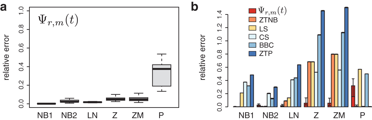
Relative errors in simulation studies. (a) Relative error of the estimator Ψ_r,m(t) for the six simulation models. Box plots are based on 1000 replicate simulations. The horizontal bar displays the median, boxes display quartiles, and whiskers depict minima and maxima. (b) Mean relative error of all tested estimators for simulated data sets based on 1000 replicates for each model. The error bars show the 95% confidence interval of relative errors. The models and the estimators are explained in detail in Section 5.

5. Simulation Studies

5.1. Models

We carried out a series of simulations to examine the performance of the estimator Ψ_r,m(t). The simulation scheme is inspired by work from Chao and Shen (2004), but involves populations and samples of larger scale. From our statistical assumptions, the number of individuals for species i in the initial sample follows a Poisson distribution with the rate λ_i, for i = 1, 2, …, L. The rates λ_i are generated from distributions we have selected to model populations with different degrees and types of heterogeneity. We describe the degree of heterogeneity in a population by the coefficient of variation (CV) for λ_i:

The CV quantifies difference in relative abundances among species and is independent of sample size. For the type of heterogeneity, we focus on the shapes of distributions, for example, distinguishing those with exponentially decreasing tails versus heavy-tailed distributions.

We selected six models for our simulations. The first is a homogenous model (P; Poisson), where all species have the same relative abundance, included as a basis for comparison with the other models. Intuitively, the homogeneous model is the simplest one among all models. However, for a given sample size, samples from the homogeneous population contain the least information among any type of population if the sample size is relatively small compared with L (see details and the proof in Supplementary Materials [Section S5]). The second and third models are negative binomials (NB1 and NB2), where the λ_i follows gamma distributions. The NB models are widely used to describe overdispersed count data (Hilbe, 2011), particularly in modeling sequencing data (Robinson and Smyth, 2007; Robinson et al., 2010; Song and Smith, 2011; McCarthy et al., 2012; Van den Berge et al., 2018). The fourth model is a lognormal (LN) model (Bulmer, 1974), which has been applied to capture–recapture analysis in ecology (Preston, 1948). Models 5 and 6 are a Zipf distribution (Z; Zipf, 1935) and a Zipf/Mandelbrot distribution (ZM; Mandelbrot, 1977), respectively, which are known as power law. Models 4–6 represent so-called heavy-tailed populations (Newman, 2005). Supplementary Table S1 in the Supplementary Materials summarizes these parameter settings.

In our simulations, we fixed the total number L of species at 1 million (M) to represent large-scale applications. For each model, the values of model parameters were determined in such that $\sum_{i = 1}^{L} λ_{i} = L = 1 M$ . In other words, the expected size of initial samples was set to 1M individuals. We use sample coverage (SC) to indicate how well a sample can represent the corresponding population. The formal definition of SC is the total proportion of species in the population that are covered in the sample. Recall that t is the amount by which we seek to extrapolate relative to the initial sample size. Our simulations cover (t, r) representing the region [1,100] × {1,…,100}, which more than represents the (t, r) we have seen in practical sequencing applications. We measure performance of estimators using relative error. For fixed r, relative error is calculated as the L²-distance between the expected $E [S_{r} (t)]$ and the estimate, divided by the L²-norm of $E [S_{r} (t)]$ , evaluated at t = 1, 2, …, 100. The errors we report are means of relative error over the curves for r = 1, 2, …, 100. We compared the estimator Ψ_r,m(t) with five other estimators: the zero-truncated Poisson (ZTP; Cohen, 1960), the zero-truncated negative binomial (ZTNB; Sampford, 1955), the logseries approch (LS; Fisher et al., 1943), and two nonparametric estimators Boneh-Boneh-Caron (BBC) (Boneh et al., 1998) and Chao-Shen (CS) (Chao and Shen, 2004). The last two estimators were designed for SACs. To use those latter estimators for r-SAC estimates, we leveraged Equation (3) in Theorem 1 to derive the general expression for $E [S_{r} (t)]$ , for r ≥ 1. Details are found in the Supplementary Materials (Section S2).

5.2. Simulation results

As can be seen from Figure 2a, the estimator Ψ_r,m(t) performs well under models NB1, NB2, LN, Z, and ZM. We consider these to represent heterogeneous populations due to their large CV compared with the homogeneous model (Supplementary Table S1). The relative errors are 0.002 (± 0.003) and 0.027 (± 0.011) for NB1 and NB2. The errors for the Z and ZM models are slightly higher: 0.057 (± 0.042) and 0.057 (± 0.040), respectively (Supplementary Table S2). Both the relative error and the standard error of Ψ_r,m(t) are much higher when applied to the homogenous models (Fig. 2a).

We compared the estimator Ψ_r,m(t) with the five other estimators. The estimator Ψ_r,m(t) has the least mean relative error compared with other approaches under the LN, Z, and ZM models (Fig. 2b), which are the heavy-tailed models. The relative errors under these three models are 0.020, 0.057, and 0.057 (Supplementary Table S2). In particular, under the Z and ZM models, the second-most accurate approach, our generalization of CS estimator, has a relative error of 0.525 and 0.558, around 10 × the error of Ψ_r,m(t). The estimator Ψ_r,m(t) has a higher standard error compared with the other methods (Fig. 2b), which we attribute broadly to its use of procedures that can introduce numerical error (e.g., to fit the Padé approximant). Even considering this variation, when Ψ_r,m(t) is at its least accurate, it remains substantially more accurate than the other methods across models LN, Z, and ZM. As expected, for models NB1 and NB2, the ZTNB approach is the most accurate because it matches the precise statistical assumptions of those simulations. Importantly, without any assumption about the latent distribution of λ_i, the estimator Ψ_r,m(t) also yields excellent accuracy in these two models, with relative errors less than 5%. The LS approach performs similarly to the ZTNB approach when the shape parameter in the NB model is close to zero, as occurs for NB2 (Fig. 2). Similarly, for the homogeneous population model, the ZTP approach is the most accurate.

We found the estimator Ψ_r,m(t) to be more accurate when the population samples correspond to heavy-tailed distributions compared with other methods. In general, these are the most challenging scenarios for accurately predicting $E [S_{r} (t)]$ (Fig. 2b). The NB2 and Z models have a similar degree of heterogeneity in terms of CV (Supplementary Table S1), but for all estimators except Ψ_r,m(t), the relative error for Z is clearly larger than the error for NB2. This difference is associated with the change from exponentially decreasing (NB2) compared with the power law distribution. For Ψ_r,m(t), the relative error remains small in both these scenarios. The above results correspond to an initial sample size of N = L, but for initial samples of 0.5L to 2L, the mean relative error changed very little for the heterogeneous models (Supplementary Fig. S1). The error only noticeably increased when the initial sample size was below 0.4L.

Clearly our estimator has larger relative errors when the samples are generated from a homogeneous model compared with other models (Fig. 2). Our initial intuition was that the homogeneous model should be easier to predict because all λ_i are constrained by a single parameter. Our simulation results show an interesting dichotomy in the performance of the methods we tested. On the one hand, nonparametric methods that do not assume an underlying Poisson have a higher relative error on the homogeneous model. For example, the relative errors are 0.5 and 0.32 for BBC and our estimator, respectively (Supplementary Table S2). On the other hand, the relative error is 0.003 for CS, which is based on the Poisson distribution. Parametric methods show similar trends. The ZTNB performs well under the homogeneous model because it can easily describe a Poisson when the shape parameter is large. Although the LS estimator is derived from the negative binomial, it assumes that the shape parameter is close to 0, so it has difficulty describing homogeneous data.

The SC provides one perspective on why the homogeneous model might present challenges for nonparametric approaches. In particular, the homogeneous model has the lowest SC compared with other models having a fixed sample size (Supplementary Materials in Section S5). Increasing the initial sample size can increase SC, which in turn improves the accuracy of our estimator. For example, when we increase the size of the initial sample from 1L to 2L, the relative error reduces to 0.123 (± 0.06).

6. Applications

scWGS is used to study genotypes of individual cells, for example, in the context of detecting mutations in tumors (Zong et al., 2012) or characterizing the landscape of mutations in normal cells (Zhang et al., 2019). Because of the inherent limited amount of DNA in any single cell, scWGS heavily relies on whole-genome amplification (WGA) to obtain enough material for sequencing. Multiple strategies exist for WGA. Early methods include exponential amplification as in degenerate oligonucleotide-primed polymerase chain reaction (Telenius et al., 1992) and multiple displacement amplifications (Dean et al., 2002; Leung et al., 2016). More recent methods avoid exponential amplification. Examples include the multiple annealing and looping-based amplification cycles (Zong et al., 2012), and the linear amplification via transposon insertion (Chen et al., 2017). Each WGA method has different amplification efficiencies and sequencing biases, resulting in different genome coverage profiles for a given amount of sequencing effort (Huang et al., 2015; Chen et al., 2017). By analyzing data with these diverse characteristics, we can examine the behavior of estimators in multiple distinct, yet realistic, settings.

We aim to predict the expected number of sites in the genome covered by at least r reads as a function of the sequencing effort (r-SAC) in a sequencing library. Therefore, for each protocol, our task is to estimate how the genome coverage changes as the sequencing effort increases. In practice, researchers are usually not interested in all values of r but particular values of r, which are defined as “sufficient” coverage based on how the data will be used in subsequent analysis steps.

We collected 10 scWGS samples from 3 studies (Zong et al., 2012; Chen et al., 2017; Dong et al., 2017). These data sets were generated in different laboratories using different protocols. Supplementary Table S3 lists the accession numbers, in the NCBI SRA database, of the sequencing runs used in this study. For each data set, we randomly downsampled a subset of 5M reads as an initial sample, and used this initial sample to predict the r-SAC (see Supplementary Materials in Section S6 for scWGS processing details). We then compared the predicted r-SAC with the ground truth, which is obtained by subsampling without replacement from the entire data set, and used relative error to assess prediction accuracy of our method.

We evaluated the accuracy of our predicted r-SAC for r ≤ 20, which is sufficient for almost all applications. Figure 3 shows the actual r-SAC along with our estimated r-SAC for r = 4, 8, 10, 20. The first thing to note is the diverse shapes associated with each distinct technology. These shapes are not necessarily a result of the technology, and might differ if we examined other data from the same technology. However, this diversity still challenges estimators in different ways. In each case, our estimated curves closely track the true curves for different values of r. Predictions from all four protocols were all generally accurate, with relative errors less than 10% for all data sets when r ≤ 10 (Table 1). We can conclude that using only 5M reads in each experiment, we are able to detect the differences in genome coverage within each of the sequencing libraries, for a variety of r values and at over 40-fold extrapolation.

FIG. 3.

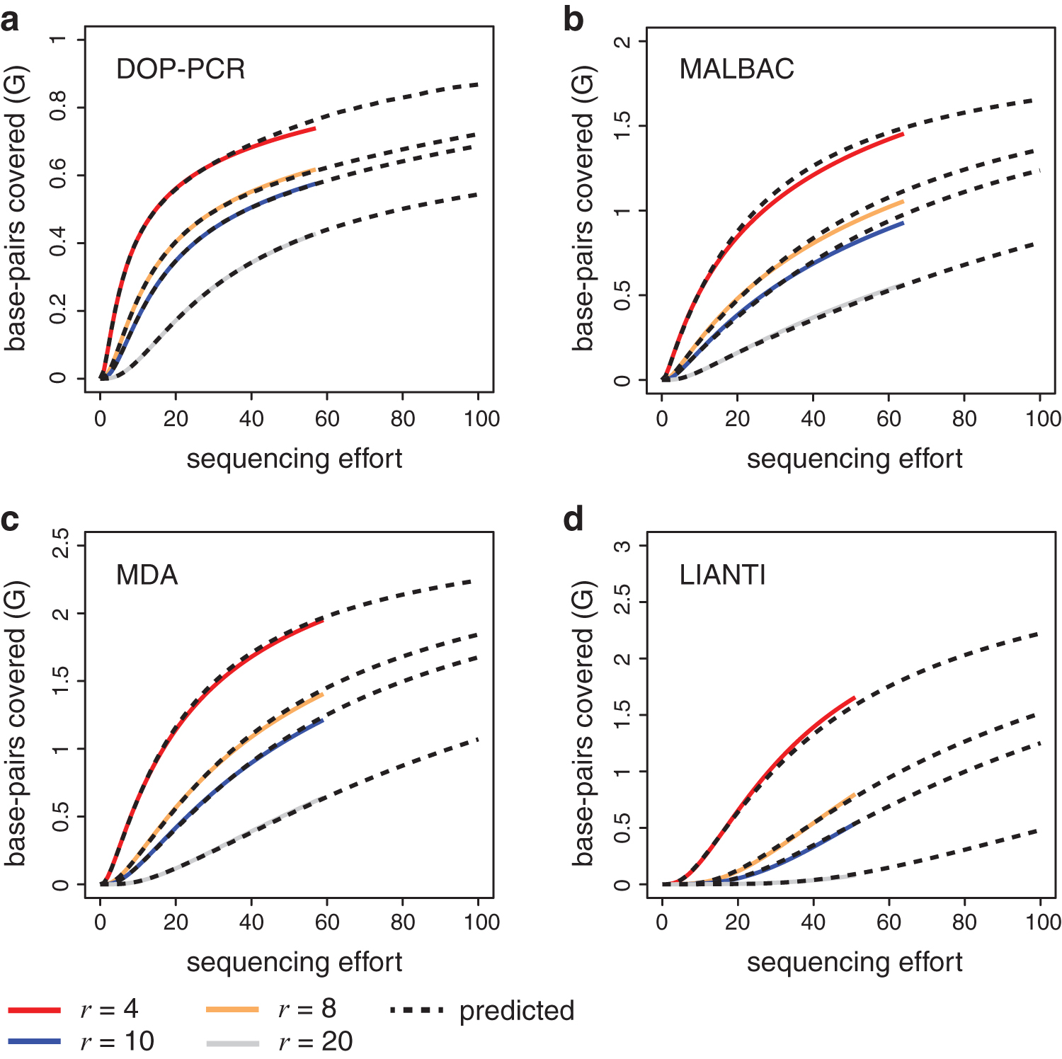
Predicted r-SACs for scWGS data sets. The number of sites in the genome covered at least r times as a function of the sequencing effort, for r = 4, 8, 10, and 20. The dashed line is the predicted curve based on Ψ_r,m(t) using an initial sample of 5M reads. The size of initial samples equals to one unit of sequencing effort. We extrapolated up to 500M reads using the initial sample. The solid line is generated by subsampling the entire data set without replacement. The accession numbers in NCBI for each data set used in the figure are as follows: (a) SRR5365365; (b) SRR5365368; (c) SRR5365371; and (d) SRR5365374. r-SAC, r-species accumulation curve; scWGS, single-cell whole-genome sequencing.

Table 1.

Relative Errors for Estimating r-Species Accumulation Curves in Single-Cell Whole-Genome Sequencing Using Ψ_r,_m(t) and Zero-Truncated Poisson

Accession id	r = 1	r = 2	r = 3	r = 4	r = 5	r = 6	r = 7	r = 8	r = 9	r = 10
Ψ_r,m(t)
SRR611492	0.020	0.011	0.006	0.004	0.004	0.005	0.006	0.007	0.009	0.010
SRR618274	0.032	0.008	0.014	0.019	0.021	0.019	0.018	0.016	0.015	0.013
SRR2976562	0.061	0.055	0.031	0.026	0.058	0.07	0.051	0.079	0.013	0.013
SRR2976563	0.002	0.001	0.001	0.001	0.000	0.001	0.002	0.002	0.001	0.002
SRR2976568	0.035	0.012	0.020	0.031	0.034	0.036	0.033	0.027	0.029	0.031
SRR2976569	0.007	0.005	0.003	0.005	0.007	0.008	0.008	0.009	0.008	0.007
SRR5365365	0.100	0.029	0.039	0.021	0.009	0.013	0.003	0.003	0.007	0.004
SRR5365368	0.080	0.025	0.025	0.038	0.045	0.048	0.048	0.045	0.042	0.036
SRR5365371	0.031	0.010	0.010	0.015	0.018	0.019	0.019	0.018	0.016	0.014
SRR5365374	0.036	0.015	0.032	0.042	0.044	0.039	0.033	0.027	0.030	0.042
ZTP
SRR611492	0.605	0.553	0.506	0.460	0.418	0.379	0.347	0.323	0.312	0.315
SRR618274	0.563	0.488	0.423	0.367	0.320	0.288	0.275	0.286	0.320	0.372
SRR2976562	0.281	0.243	0.208	0.180	0.166	0.176	0.211	0.264	0.330	0.403
SRR2976563	0.357	0.303	0.257	0.219	0.197	0.197	0.223	0.270	0.329	0.397
SRR2976568	0.254	0.223	0.194	0.170	0.158	0.167	0.199	0.252	0.318	0.392
SRR2976569	0.314	0.265	0.224	0.191	0.174	0.178	0.204	0.249	0.306	0.369
SRR5365365	0.581	0.444	0.379	0.336	0.304	0.278	0.258	0.244	0.235	0.232
SRR5365368	0.623	0.547	0.484	0.429	0.381	0.341	0.311	0.293	0.288	0.297
SRR5365371	0.522	0.449	0.385	0.331	0.288	0.261	0.257	0.278	0.318	0.372
SRR5365374	0.407	0.303	0.213	0.198	0.297	0.454	0.628	0.796	0.938	1.032

ZTP, zero-truncated Poisson.

We compared our estimation method with both parametric and nonparametric methods that are listed above for the simulation study. The estimator Ψ_r,m(t) has clearly superior performance among these methods. Table 1 and Supplementary Table S4 show the relative errors of each method for r from 1 to 10. Overall, the number of cases where the relative error of Ψ_r,m(t) is higher than other methods is fewer than 2%. In particular, our estimator has a lower relative error than estimators ZTP, CS, and BBC for all values of r ≤ 10 across all data sets. Furthermore, the relative errors of the estimator Ψ_r,m(t) are less than 10% across all data sets for all r ≤ 10 (Table 1). In contrast, the ZTNB, which shows the second-best performance, has a relative error of 30.3% at r = 1 for the data set SRR2976568 (Supplementary Table S4).

7. Discussion

We introduced a new approach to estimate the genome coverage as a function of the sequencing effort. The nonparametric estimators obtained by our approach are universal in the sense that they apply across values of r for a given sequencing library. We have shown that these estimators have favorable properties in theory, and also give highly accurate estimates in practice. Accuracy remains high for large values of r and for long-range extrapolations. This approach builds on the theoretical nonparametric empirical Bayes foundation of Good and Toulmin (1956), providing a practical way to compute estimates that are both accurate and stable.

We discovered a relationship between the r-SAC $E [S_{r} (t)]$ and the SAC $E [S_{1} (t)]$ , which are connected using (r – 1)th derivative. This relationship can generalize any smooth expression of an SAC to its corresponding r-SAC and therefore enables the extension of existing estimators for the SAC. This relationship is especially helpful for nonparametric methods for which the expression might otherwise appear tailed specifically to the case r = 1. We derived several estimators for r-SACs and evaluated their performance through large-scale simulation studies. All the estimators have been implemented in an R package called preseqR (v.4.0.0). Therefore, one can easily use these estimators in genomic sequencing, ecology, linguistics, or other domains, which use capture–recapture analysis. The package is available through CRAN at: https://CRAN.R-project.org/package=preseqR

For large-sequencing projects, such as the international 1000 Genomes Project (The 1000 Genomes Project Consortium, 2015) and the UK 100,000 Genomes Project (Genomics England, 2017), one crucial question is how to balance between the number of individuals in the study and the sequencing effort for each individual. Under a fixed budget, we should aim to sequence as many individuals as possible to enhance the statistical power of the study, while still ensuring that the sequencing in each sample is sufficient to make confident estimates about genotype. Having a small but sufficient sequencing sample also largely saves computing time and data storage. Using a shallow sequencing experiment as a pilot study, our method provides an accurate estimation for the genome coverage in the future large-sequencing sample, and helps scientists plan the sequencing effort for various protocols.

For modern biological sequencing applications, samples are frequently in the millions, and the scale of the data could be different by orders of magnitude. These large-scale applications present new challenges to traditional capture–recapture statistics, and call for methods that can integrate high-order moments to accurately characterize the underlying population. We generalized the classical study of estimating an SAC and propose a nonparametric estimator that can theoretically leverage any number of moments. Both this generalization and the associated methodology suggest possible avenues for practical advances in related estimation problems. Particularly in the context of genomic sequencing, we believe that this perspective will play important roles of experimental planning in the big genome projects, as well as accelerating the development process of new sequencing methods.

Footnotes

Author Disclosure Statement

The authors are not aware of any affiliations, memberships, funding, or financial holdings that might be perceived as affecting the objectivity of this review.

Funding Information

This work was supported by the NIH/NHGRI (National Institutes of Health/National Human Genome Research Institute) R01 HG007650 (A.D.S.).

Supplementary Material

References

Baker

G.A.

, and Graves-Morris

P.R.

1996. Padé Approximants. Cambridge University Press, Cambridge.

Benjamini

, and Speed

T.P.

2012). Summarizing and correcting the GC content bias in high-throughput sequencing. Nucleic Acids Res. 40, e72.

Bhattacharya

S.K.

1966. Confluent hypergeometric distributions of discrete and continuous type with applications to accident proneness. Calcutta Stat. Assoc. Bull. 15, 20–31.

Boneh

, Boneh

, and Caron

R.J.

1998. Estimating the prediction function and the number of unseen species in sampling with replacement. J. Am. Stat. Assoc. 93, 372–379.

Bulmer

M.G.

1974. On fitting the poisson lognormal distribution to species-abundance data. Biometrics, 30, 101–110.

Burrell

Q.L.

, and Fenton

M.R.

1993. Yes, the GIGP really does work—And is workable! J. Am. Soc. Inf. Sci. 44, 61–69.

Chao

1987. Estimating the population size for capture-recapture data with unequal catchability. Biometrics, 43, 783–791.

Chao

, and Shen

T.-J.

2004. Nonparametric prediction in species sampling. J. Agr. Biol. Environ. Stat. 9253–269.

Chen

, Xing

, Tan

, et al. 2017. Single-cell whole-genome analyses by Linear Amplification via Transposon Insertion (LIANTI). Science, 356, 189–194.

10.

Cohen

A.C.

1960. Estimating the parameters of a modified Poisson distribution. J. Am. Stat. Assoc. 55, 139–143.

11.

Daley

2014. Non-Parametric Models for Large Capture-Recapture Experiments with Applications to DNA Sequencing. PhD thesis, University of Southern California.

12.

Daley

, and Smith

A.D.

2013. Predicting the molecular complexity of sequencing libraries. Nat. Methods, 10, 325–327.

13.

Daley

, and Smith

A.D.

2014. Modeling genome coverage in single-cell sequencing. Bioinformatics, 30, 3159–3165.

14.

Dean

F.B.

, Hosono

, Fang

, et al. 2002. Comprehensive human genome amplification using multiple displacement amplification. Proc. Natl. Acad. Sci. 99, 5261–5266.

15.

Deng

, Daley

, and Smith

2015. Applications of species accumulation curves in large-scale biological data analysis. Quant. Biol. 3, 135–144.

16.

Dong

, Zhang

, Milholland

, et al. 2017. Accurate identification of single-nucleotide variants in whole-genome-amplified single cells. Nat. Methods, 14, 491–493.

17.

Eboreime

, Choi

S.-K.

, Yoon

S.-R.

, et al. 2016. Estimating exceptionally rare germline and somatic mutation frequencies via next generation sequencing. PLoS One, 11, e0158340.

18.

Efron

, and Thisted

1976. Estimating the number of unsen species: How many words did Shakespeare know?. Biometrika, 63, 435–447.

19.

Efron

, and Tibshirani

R.J.

1994. An Introduction to the Bootstrap. Chapman & Hall, London.

20.

Engen

1978. Stochastic Abundance Models. Chapman and Hall, London.

21.

Fisher

R.A.

, Corbet

A.S.

, and Williams

C.B.

1943. The relation between the number of species and the number of individuals in a random sample of an animal population. J. Anim. Ecol. 12, 42–58.

22.

Genomics England. 2017. The 100,000 Genomes Project. Available at: https://www.genomicsengland.co.uk/the-100000-genomes-project. Accessed May 4, 2019.

23.

Good

I.J.

1953. The population frequencies of species and the estimation of population parameters. Biometrika, 40, 237–264.

24.

Good

I.J.

, and Toulmin

G.H.

1956. The number of new species, and the increase in population coverage, when a sample is increased. Biometrika, 43, 45–63.

25.

Hilbe

J.M.

2011. Negative Binomial Regression. Cambridge University Press, Cambridge.

26.

Huang

, Ma

, Chapman

, et al. 2015. Single-cell whole-genome amplification and sequencing: Methodology and applications. Annu. Rev. Genom. Hum. Genet. 16, 79–102.

27.

Kalinin

V.M.

1965. Functionals related to the Poisson distribution, and statistical structure of a text. Proc. Steklov Inst. Math. 79, 6–19.

28.

Lander

E.S.

, and Waterman

M.S.

1988. Genomic mapping by fingerprinting random clones: A mathematical analysis. Genomics, 2, 231–239.

29.

Leung

, Klaus

, Lin

B.K.

, et al. 2016. Robust high-performance nanoliter-volume single-cell multiple displacement amplification on planar substrates. Proc. Natl. Acad. Sci. 113, 8484–8489.

30.

Mandelbrot

B.B.

1977. Fractals: Forms, Chance and Dimension. Freeman, San Francisco.

31.

McCarthy

D.J.

, Chen

, and Smyth

G.K.

2012. Differential expression analysis of multifactor RNA-Seq experiments with respect to biological variation. Nucleic Acids Res. 40, 4288–4297.

32.

Newman

M.E.

2005. Power laws, Pareto distributions and Zipf's law. Contemp. Phys. 46, 323–351.

33.

S.B.

, Buckingham

K.J.

, Lee

, et al. 2010. Exome sequencing identifies the cause of a mendelian disorder. Nat. Genet. 42, 30–35.

34.

Preston

F.W.

1948. The commonness, and rarity, of species. Ecology, 29, 254–283.

35.

Rahman

Q.I.

, and Schmeisser

2002. Analytic Theory of Polynomials. Oxford University Press, Oxford.

36.

Robinson

M.D.

, McCarthy

D.J.

, and Smyth

G.K.

2010. edgeR: A Bioconductor package for differential expression analysis of digital gene expression data. Bioinformatics, 26, 139–140.

37.

Robinson

M.D.

, and Smyth

G.K.

2007. Small-sample estimation of negative binomial dispersion, with applications to SAGE data. Biostatistics, 9, 321–332.

38.

Sampford

M.R.

1955. The truncated negative binomial distribution. Biometrika, 42, 58–69.

39.

Sanger

, Nicklen

, and Coulson

A.R.

1977. DNA sequencing with chain-terminating inhibitors. Proc. Natl. Acad. Sci. 74, 5463–5467.

40.

Sichel

H.S.

1975. On a distribution law for word frequencies. J. Am. Stat. Assoc. 70, 542–547.

41.

Sims

, Sudbery

, Ilott

N.E.

, et al. 2014. Sequencing depth and coverage: Key considerations in genomic analyses. Nat. Rev. Genet. 15, 121–132.

42.

Song

, and Smith

A.D.

2011. Identifying dispersed epigenomic domains from ChIP-Seq data. Bioinformatics, 27, 870–871.

43.

Telenius

, Carter

N.P.

, Bebb

C.E.

, et al. 1992. Degenerate oligonucleotide-primed PCR: General amplification of target DNA by a single degenerate primer. Genomics, 13, 718–725.

44.

The 1000 Genomes Project Consortium. 2012. An integrated map of genetic variation from 1,092 human genomes. Nature, 491, 56–65.

45.

The 1000 Genomes Project Consortium. 2015. A global reference for human genetic variation. Nature, 526, 68–74.

46.

Van den Berge

, Perraudeau

, Soneson

, et al. 2018. Observation weights unlock bulk RNA-seq tools for zero inflation and single-cell applications. Genome Biol. 19, 24.

47.

2018. A review of somatic single nucleotide variant calling algorithms for next-generation sequencing data. Comput. Struct. Biotechnol. J. 16, 15–24.

48.

Zhang

, Dong

, Lee

, et al. 2019. Single-cell whole-genome sequencing reveals the functional landscape of somatic mutations in b lymphocytes across the human lifespan. Proc. Natl. Acad. Sci. 116, 9014–9019.

49.

Zipf

G.K.

1935. The Psycho-Biology of Language. Houghton Mifflin, Boston.

50.

Zong

, Lu

, Chapman

A.R.

, et al. 2012. Genome-wide detection of single-nucleotide and copy-number variations of a single human cell. Science, 338, 1622–1626.

Supplementary Material

Please find the following supplemental material available below.

For Open Access articles published under a Creative Commons License, all supplemental material carries the same license as the article it is associated with.

For non-Open Access articles published, all supplemental material carries a non-exclusive license, and permission requests for re-use of supplemental material or any part of supplemental material shall be sent directly to the copyright owner as specified in the copyright notice associated with the article.

0.00 MB

0.38 MB