A Robustness Analysis of Dynamic Boolean Models of Cellular Circuits

Abstract

With ever growing amounts of omics data, the next challenge in biological research is the interpretation of these data to gain mechanistic insights about cellular function. Dynamic models of cellular circuits that capture the activity levels of proteins and other molecules over time offer great expressive power by allowing the simulation of the effects of specific internal or external perturbations on the workings of the cell. However, the study of such models is at its infancy and no large-scale analysis of the robustness of real models to changing conditions has been conducted to date. Here we provide a computational framework to study the robustness of such models using a combination of stochastic simulations and integer linear programming techniques. We apply our framework to a large collection of cellular circuits and benchmark the results against randomized models. We find that the steady states of real circuits tend to be more robust in multiple aspects compared with their randomized counterparts.

1. Introduction

Protein–protein interaction networks have been mapped for over a decade using techniques such as yeast two-hybrid and coimmunoprecipitation. Comprehensive maps are available for multiple species, including yeast and human, with hundreds of thousands of interactions in each [see e.g., the BioGRID database (Chatr-Aryamontri et al., 2015)]. As we and others have shown, substantial portions (over 40%) of those maps are spanned by signaling interactions (Silberberg et al., 2014). Thus, protein networks have been extensively used for interpreting genome-wide screens in the context of a phenotype of interest. Previous work in this regard can be broadly categorized into topology based and logic based. The first category includes the vast majority of current studies. It aims to characterize a given phenotype by the following: (i) the location of its affected proteins in a network, identifying network regions, or modules that are associated with the phenotype (Ideker et al., 2002; Dittrich et al., 2008; Shachar et al., 2008; Huang and Fraenkel, 2009; Yeger-Lotem et al., 2009; Yosef et al., 2009; Vandin et al., 2011; Cowen et al., 2017); and (ii) the network-based attributes of the proteins, such as degree of connectivity and more (Said et al., 2004; Jonsson and Bates, 2006).

The second logic-based category aims to provide mechanistic models for the phenotype of interest (Novere, 2015). While a variety of models can be used, most prior works focus on logical (Boolean) models or variations thereof (Morris et al., 2010), thanks to the rich history of these models in the biological domain (Kauffman, 1969). These works include Boolean modeling of fundamental systems such as epidermal growth factor receptor (EGFR) signaling (Oda et al., 2005; Samaga et al., 2009) and mitogen-activated protein kinase (MAPK) signaling (Grieco et al., 2013); algorithms to optimize Boolean models against experimental data (Mitsos et al., 2009; Saez-Rodriguez et al., 2009; Moignard et al., 2015); algorithms to traverse the state space of a model (Dubrova and Teslenko, 2011; Chaouiya et al., 2012; Qiu et al., 2014); and generalizations of these models to multivalued (Morris et al., 2011; Huard et al., 2012), constraint-based (Dasika et al., 2006; Vardi et al., 2012), and probabilistic (Gat-Viks et al., 2006) ones.

The advantage of the latter logic-based models is that they allow simulating a process of interest under different genetic and environmental perturbations. In recent years, a concentrated community effort has led to the curation of dozens of logic models for a diverse array of cellular processes (Ideker et al., 2002), providing for the first time the opportunity to study the properties of these circuits at large scale.

Since biological processes need to operate consistently in a noisy environment, they must be robust to perturbations, such as stochastic changes in molecular concentrations and protein activity. Extensive research has been done on empirical stability of biological processes (Alon et al., 1997; Li et al., 2004), as well as stability of Boolean models (Aldana and Cluzel, 2003; Sevim and Rikvold, 2008; Fretter et al., 2009; Peixoto, 2010; Schwab et al., 2017) and alternative modeling frameworks (Chen and Aihara, 2002, 2006; Klemm and Bornholdt, 2002, 2005; Lyapunov, 2007; Chaves et al., 2008).

However, there are few studies that compare the robustness of real networks to those of random networks with similar structural properties. Indeed, random networks can be artificially selected for robustness, affecting their structural properties (Sevim and Rikvold, 2008; Fretter et al., 2009). We are aware of only a single work that directly compares real networks to topologically similar random ones. Specifically, Daniels et al. (2018) compared 67 biological models with topologically and functionally similar random models, identifying a node-based sensitivity measure that differs between the two types of models.

Here, for the first time, we compare real and similar random models in terms of their dynamical properties. Since the space of model states is exponentially large, mapping its attractors and basins of attraction is very costly. To tackle this computational problem, we design novel integer linear programming (ILP) formulations for model learning and attractor computations. We apply our methodology to a set of 30 curated models covering fundamental biological processes in multiple species with up to 62 nodes. We analyze their steady-state (attractor) properties and their robustness to small perturbations. As a benchmark, we use randomized models that maintain the topology and logical complexity of the real models. We find that real models tend to be more robust than random models in several aspects that concern the steady-state changes in response to intrinsic noise in the system or due to small perturbations to its logic.

2. Preliminaries

For a cell circuit of interest, a Boolean model is a pair $(G, F)$ , where $G = (V, E)$ is a directed graph representing the circuit topology with $n = | V |$ nodes and F is a collection of Boolean functions over V. To define F, let us denote, for each $v_{i} \in V$ , the ordered set $p (v_{i}) = (v_{j} : (v_{j}, v_{i}) \in E)$ , with an arbitrary order over V. Let $f_{i} : {0, 1}^{| p (v_{i}) |} \to {0, 1}$ be a Boolean function representing the activity of v_i in terms of its predecessors $p (v_{i})$ .

An assignment of binary activity levels to each node defines a state of the model. We assume a synchronous model, where for each discrete time point t and vertex v_i, $v_{i, t} \in {0, 1}$ defines the vertex activity at time t, for an arbitrary starting value $v_{i, 0}$ . Denote $p_{t} (v_{i}) = (v_{j, t} : v_{j} \in p (v_{i}))$ , then the model is updated as follows (for all $v_{i} \in V$ and $t \geq 0$ ): $v_{i, (t + 1)} = f (v_{i, t}) : = \{\begin{matrix} v_{i, t} & | p (v_{i}) | = 0 \\ f_{i} (p_{t} (v_{i})) & o t h e r w i s e \end{matrix}$ (1)

An attractor for G is a simple cycle of network states. Formally, a state path A of length T is a tuple $(V_{t} : 0 \leq t \leq T)$ where each $V_{t} = (v_{i, t} : v_{i} \in V)$ represents a state and Equation (1) holds for each $0 \leq t < T$ . We say that A is an attractor if $V_{T} = V_{0}$ and for all other t, $V_{t} \neq V_{0}$ . By definition, every state in a synchronous model is followed by exactly one state, and hence, every state leads to a single attractor. For a given attractor, we call the set of states that lead to this attractor its basin of attraction, and use the notation $s \to A$ to mean that s is in the basin of attraction of A.

3. Methods

To test the robustness of a given model, we examine the impact of small perturbations on its dynamics. Specifically, we consider two types of perturbations: (i) changing k bits in the truth tables of one or more of its functions, where k is a small constant; (ii) switching from any state to another state whose Hamming distance to the original is at most k. We study the impact of such changes on the set of model attractors by quantifying for each change the percent of model states, leading to a different attractor in the perturbed model/state.

Since the space of model states is exponentially large, mapping its attractors and basins of attraction is very costly. To tackle this computational problem, we combine novel ILP formulations for model learning and attractor computations with stochastic simulations for estimating the size of each basin of attraction. To describe our formulation for attractor representation, we first describe a set of subprograms that form its building blocks.

3.1. State comparisons

The representation of attractor states requires efficient means to compare them to one another to make sure that they represent a cyclic path of distinct states and that no two attractors share the same state. One way to tackle this problem as well as remove degrees of freedom from solutions is to assign a unique numeric key to each possible network state. The resulting order can then be used to implement equality and inequality constraints.

A natural key for a state is the binary number it represents, but the representation size may exceed the number of bits in a computer word. Instead, we implement this representation by assuming an arbitrary upper bound of M bits per word and splitting the number into $ℓ + 1$ pieces, where $ℓ : = ⌈\frac{| V |}{M}⌉ - 1$ . For any two states $a, b \in {0, 1}^{| V |}$ represented by $x_{0}, \dots x_{ℓ}$ and $y_{0}, \dots, y_{ℓ}$ , respectively, to implement an indicator for an inequality such as $a > b$ , we use auxiliary binary variables $(z_{0}, \dots, z_{ℓ})$ and, for convenience, denote $z_{- 1} = 0$ . We introduce the following constraints for all $0 \leq j \leq ℓ$ : $\begin{matrix} (2^{M} + 1) z_{j} \geq x_{j} - y_{j} + z_{j - 1} \\ (2^{M} + 1) z_{j} \leq x_{j} - y_{j} + z_{j - 1} + 2^{M} . \end{matrix}$ (2)

It holds that $z_{0} = 1$ iff (if and only if) $x_{0} > y_{0}$ and for $j \geq 1$ : $z_{j} = 1 \Leftrightarrow x_{j} > y_{j} \lor (x_{j} = y_{j} \land z_{j - 1} = 1) .$

This implies that $z_{ℓ} = 1$ iff $a > b$ , and we can denote $I_{a > b} = z_{ℓ}$ . Using $z_{- 1} = 1$ captures a weak ordering and allows us to implement the indicators $I_{a = b}$ and $I_{a \neq b}$ as well.

We can use these indicators to implement a set membership indicator $I_{a \in A}$ representing whether a state a belongs to a set of states A, with the formulation: $\begin{matrix} \forall a' \in A : I_{a \in A} \geq I_{a = a'} \\ I_{a \in A} \leq \sum_{a' \in A} I_{a = a'} \end{matrix} .$

3.2. Path constraints

Let $a_{0}, \dots, a_{T}$ be ordered sets of binary vector variables, representing graph states, such that $\forall t, a_{t} = (v_{1, t}, \dots, v_{n, t})$ . Let $F (a_{t}) = (f (v_{1, t}), \dots, f (v_{n, t}))$ , then we can enforce the ordered set of states to represent a path by requiring $a_{t + 1} = F (a_{t})$ for all $t < T$ . We follow the technique used in Sharan and Karp (2006) as detailed below.

For an input node v_i such that $| p (v_{i}) | = 0$ , we only require $v_{i, t + 1} = v_{i, t}$ . Otherwise, denote by i_j the index of the jth node in $p (v_{i})$ . For each binary vector $r \in {0, 1}^{| p (v_{i}) |}$ , representing a possible input, we create an auxiliary non-negative variable s_r whose value is 0 iff r is the input vector to v_i at time $t + 1$ , that is, $r = p_{t} (v_{i})$ : $\begin{array}{l} s_{r} = | p (v_{i}) | - \sum_{j} (1 - r_{j} + v_{i_{j}, t} (2 r_{j} - 1)) \\ \begin{matrix} v_{i, t + 1} \geq f_{i} (r) - s_{r} \\ v_{i, t + 1} \leq f_{i} (r) + s_{r} . \end{matrix} \end{array}$ (3)

We call this subprogram $P A T H (a_{0}, \dots, a_{T})$ . For the case of a length −1 path, we use the simpler expression $a_{1} = F (a_{0})$ to refer to this subprogram. We can also derive a formulation for requiring the states not to form a path, which we denote by $\bar{P A T H} (a_{0}, \dots, a_{T})$ .

3.3. Attractor learning

We are now ready to present our formulations for attractor learning under various constraints. Using fixed values for the outputs of F, we can use such formulations to compute the attractors of a given model. By substituting the outputs of F with binary variables, we get a formulation whose solution represents a possible model on G and its attractors. For brevity, in the following formulations whenever we write an indicator as a constraint, we require its value to be 1. All formulations depend on specifying in advance the upper bounds on the number and length of the model's attractors. For clarity, we assume at first that there are exactly K attractors of length T each. We apply the conditional constraint mechanism below to generalize the formulations to the case that K and T are upper bounds.

Let ${a_{k, t}}_{1 \leq k \leq K, 0 \leq t \leq T}$ denote ordered sets of binary vector variables representing the K attractors. That is, each $a_{k, t}$ is a vector of n binary variables denoting the state of attractor k at time t. These variables can be populated using the following formulation (with empty objective): $M a x \lor s . t .$ $\begin{matrix} \forall k \leq K : P A T H (a_{k, 0}, \dots, a_{k, T}) \\ \forall k \leq K : I_{a_{k, 0} = a_{k, T}} \\ \forall k \leq K, t > 0 : I_{a_{k, T} > a_{k, t}} \\ \forall k < K : I_{a_{k + 1, T} > a_{k, T}}, & (4) \end{matrix}$

where degrees of freedom in attractor representation are eliminated by forcing the final state of each attractor to be the largest in terms of its associated numeric value, and the final states of different attractors to be ordered as well.

To generalize the program from $T, K$ being exact numbers to upper bounds, we introduce activity variables $w_{k, t}$ for each state $a_{k, t}$ , with $w_{k, - 1} = 0$ for all k. These activity variables affect which constraints are in effect and what variables are zeroized. Their application to the program requires a conditioning construct that enforces a constraint conditioned on the value of the activity variables. Such conditioning can be constructed by inequality constraints that take effect iff the condition is met. For example, we can formulate the constraint $a \to b \geq c$ , which requires $b \geq c$ iff $a = 1$ , by the modified constraint $b \geq c - (1 - a)$ . The generalized formulation is as follows: $M a x \lor s . t .$ $\begin{matrix} \forall k, t < T : (w_{k, t} \land w_{k, t + 1}) \to a_{k, t + 1} = F (a_{k, t}) \\ \forall k, t < T : (w_{k, t} \land \neg w_{k, t - 1}) \to I_{a_{k, 0} = a_{k, T}} \\ \forall k, t > 0 : w_{k, t} \to I_{a_{k, T} > a_{k, t}} \\ \forall k < K : (w_{k, T} \land w_{k + 1, T}) \to I_{a_{k + 1, T} > a_{k, T}} \\ \forall k, t < T - 1 : w_{k, t} \leq w_{k, t + 1} \\ \forall k < K : w_{k, T} \leq w_{k + 1, T} \\ \forall k : w_{k, T - 1} = w_{k, T} \\ \forall k, t : \neg w_{k, t} \to I_{a_{k, t} {= 0}^{n}}, & (5) \end{matrix}$

where $0^{n}$ denotes a vector of n zeros and the last constraint results in zeroizing variables that are not in use.

3.4. Robustness to state perturbations

To quantify robustness, we first consider the sensitivity of a model to small perturbations to its current state, similar to Fretter et al. (2009); Sevim and Rikvold (2008); and Ghanbarnejad and Klemm (2012). As attractors represent the steady states or behaviors of the system under study, it is natural to consider the ability of a perturbation to alter the system's behavior. Such perturbations could occur due to the inherent noise in the biological system.

Let $(G, F)$ be a given model with a set ATT of attractors. Given a state a of an attractor A, we consider perturbations of k of its bits corresponding to a set S of nodes. We denote the perturbed state by $X O R (a, S) ⁄ \to A$ . We say that a is sensitive to S if. We say that A is sensitive to S if there exists such $a \in A$ .

We evaluate the robustness of a model by a weighted average of its sensitive attractors, where attractors are weighted by their basin size estimate and the result is averaged over multiple choices of S, constrained to have cardinality k. The procedure is as follows:

Algorithm 1: Stochastic state sensitivity score

1. Calculate model attractors.

2. Sample a state s and a node set S uniformly at random.

3. Simulate the model from s to derive its attractor A.

4. Sample a state

a \in A

uniformly at random.

5. Simulate the model from

X O R (a, S)

to determine A's sensitivity to S.

6. Repeat steps (1–5) 200 times and average the sensitivity results.

As an alternative sensitivity measure, we use an ILP formulation to compute an upper bound rather than an average on sensitivity. That is, we find the maximal weighted average of attractors that are sensitive to a set S of a given cardinality. Denote the relative basin size of attractor $A \in A T T$ by $w_{A} : = | {s \in {0, 1}^{n} : s \to A} | ∕ 2^{n}$ . We can use the stochastic procedure above to estimate w_A for each $a \in A T T$ . For the formulation, we further assume that any state reaches its attractor after at most P steps. We denote the set of attractor states by R. We represent the perturbed set S by binary variables $s_{1}, \dots, s_{n}$ , and formulate the following program: $M a x \sum_{A \in A T T} w_{A} \cdot I_{b_{P}^{A} \in R ∖ A} s . t .$ $\begin{matrix} \sum_{i} s_{i} \leq k \\ \forall A \in A T T : I_{a^{A} \in A} \\ \forall A \in A T T : I_{b_{0}^{A} = X O R (a^{A}, S)} \\ \forall A \in A T T : P A T H (b_{0}^{A}, \dots, b_{P}^{A}) . \end{matrix}$

3.5. Robustness to logic perturbations

An orthogonal way to measure the robustness of a model is by the effects of perturbing its logical functions on the model's attractors (Li et al., 2004; Sevim and Rikvold, 2008). As before, we assume that up to k bits are changed in the truth tables of the Boolean functions.

Let $(G, F)$ be a source model with a set ATT of attractors and let $(G, F')$ be the perturbed model with a set $A T T'$ of attractors. We consider the percent of model states whose associated attractors were eliminated by the change: $\sum_{A \in A T T ∖ A T T'} w_{A}$ . For brevity, we omit the constraint regarding the number of bit changes. $M a x \sum_{A \in A T T} w_{A} \cdot I_{A} s . t .$

\begin{matrix} \forall A \in A T T : I_{A} = 1 \to \bar{P A T H (A)} \\ \forall A \in A T T : I_{A} = 0 \to P A T H (A) . \end{matrix}

To estimate the average rather than maximum sensitivity to changes, we use a stochastic procedure similar to the above.

4. Results

4.1. Data retrieval and implementation details

We downloaded 76 Boolean models from the CellCollective repository (Helikar et al., 2012), using the truth tables' export features. We excluded three models with missing information or could not be parsed and three models with acyclic graphs (hence, no dynamic behavior).

For each model, we applied four scoring variants quantifying the sensitivity of the model to state changes (stochastic and ILP-based variants) and attractor elimination due to function changes (stochastic and ILP-based variants). We used 1000 iterations to estimate each model's attractors and their basin sizes. For stochastic measures, we used 200 iterations per model. For optimization variants, we set the bound on the path length to an attractor to be $P = 1$ (the results were qualitatively similar for $P = 10$ ). We explored different values of the number k of bit changes. The results followed similar trends when k ranged from 1 to 4, we focus the description on $k = 1$ .

We benchmarked the sensitivity of the different models against randomized models in which both topology and logic functions are randomized. Specifically, the topology was randomized while preserving in- and out-degrees using the switching method with $10 n$ switch attempts; the Boolean functions were randomized while preserving the number of 1s in their truth tables by permuting table rows. We generated 40 random models for each real model.

We split the processing jobs among five servers. Two with 72 CPUs (2300 MHz) and 258 GB RAM, and the remaining three with 40 CPUs (2800 MHz) and 258 GB RAM. When running the stochastic algorithms, we ran iterations in parallel, and let the ILP solver (Gurobi) utilize all cores. Table 1 provides running time statistics. Running times varied considerably between models, and thus, we set a time-out of 90 minutes (in addition to ILP problem setup time) for running the different scoring methods on each model and discarded the results for models on which the computation was not completed within the given time bound. Overall, we collected results for 30 of the 70 models. The source code used for the analysis can be found at github.com/arielbro/attractor_learning, commit hash cd0874b6103f142ae3bb828e565e6162e7ff2f0e

Table 1.

Running Times in Seconds of the Different Scoring Variants

Variant	Median	Mean	Max
Model change, ILP	0	1	11
Model change, stochastic	27	83	1917
State change, ILP	14	322	6728
State change, stochastic	6	38	1371

ILP, integer linear programming.

4.2. Real models are more robust than their randomized counterparts

We applied our robustness computation pipeline to the 30 models described above and compared the results with those obtained on randomized models. When applying the ILP-based sensitivity analysis of model changes, we observed that in almost all cases (for both real and random models) a single bit change was enough to eliminate the entire attractor space of a model. Thus, we computed an alternative score where the change is constrained to a specific node at a time, producing a sensitivity score for each of the model's nodes, and modified the stochastic version similarly.

The distributions of the four score variants on real and random models are given in Figure 1. Evidently, real models have lower sensitivity scores than random models across all score variants. To quantify the deviation of the real models from the corresponding distributions of random scores, we used a Wilcoxon signed-rank test, where the score of each real model was paired with the mean score of its random counterparts. For the node-based model perturbation scores, we paired the mean score of vertices in a real model with the mean scores of nodes in its random counterparts.

FIG. 1.

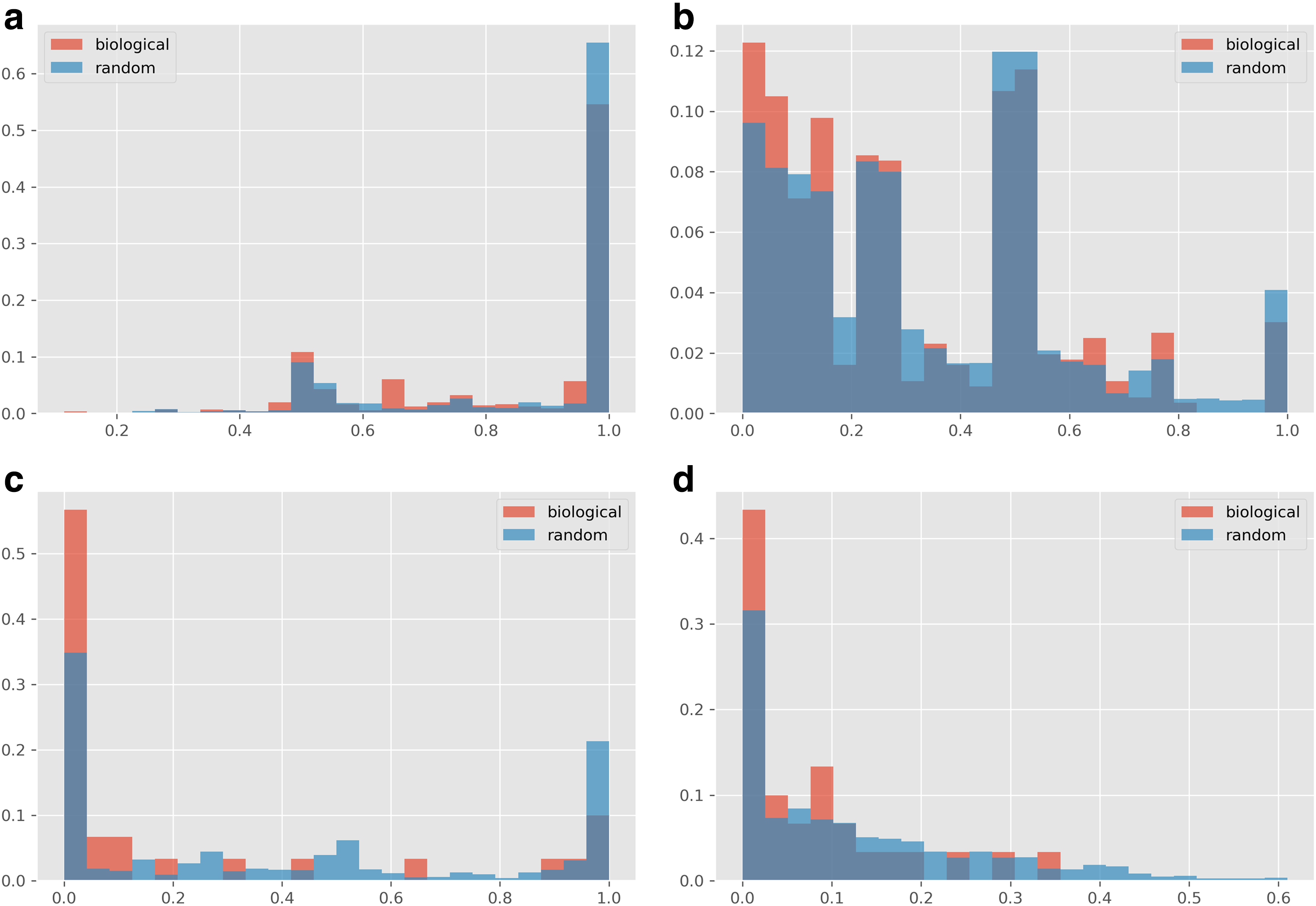
Distribution of model scores for each score variant, comparing real and random models. (a) ILP per-node scores for model perturbation. (b) Stochastic per-node scores for model perturbation. (c) ILP scores for state perturbation. (d) Stochastic scores for state perturbation. ILP, integer linear programming.

The comparison results are summarized in Table 2, revealing that in all cases the real models are more robust to changes than their randomized instances. These differences were significant for all score types ( $p < 0.05$ ), and especially for the state changes ( $p < 0.005$ ), as also evident from the box plots in Figure 2.

FIG. 2.

Box plots showing the distribution of sensitivity scores for each base network. Whiskers denote furthest data point within 1.5 IQR from median. Red dots denote the real models, and for per-node scores, the mean of real model node scores. (a) ILP per-node scores for model perturbation. (b) Stochastic per-node scores for model perturbation. (c) ILP scores for state perturbation. (d) Stochastic scores for state perturbation. IQR, interquartile range.

Table 2.

Comparison of Mean Sensitivity Scores for Real and Random Models

Variant	Real	Random	p
Model change, ILP (nodes)	0.837	0.863	0.049
Model change, stochastic (nodes)	0.311	0.339	0.017
State change, ILP	0.226	0.416	3.89e-03
State change, stochastic	0.073	0.126	8.35e-04

4.3. Stochastic versus optimization-based sensitivity analysis

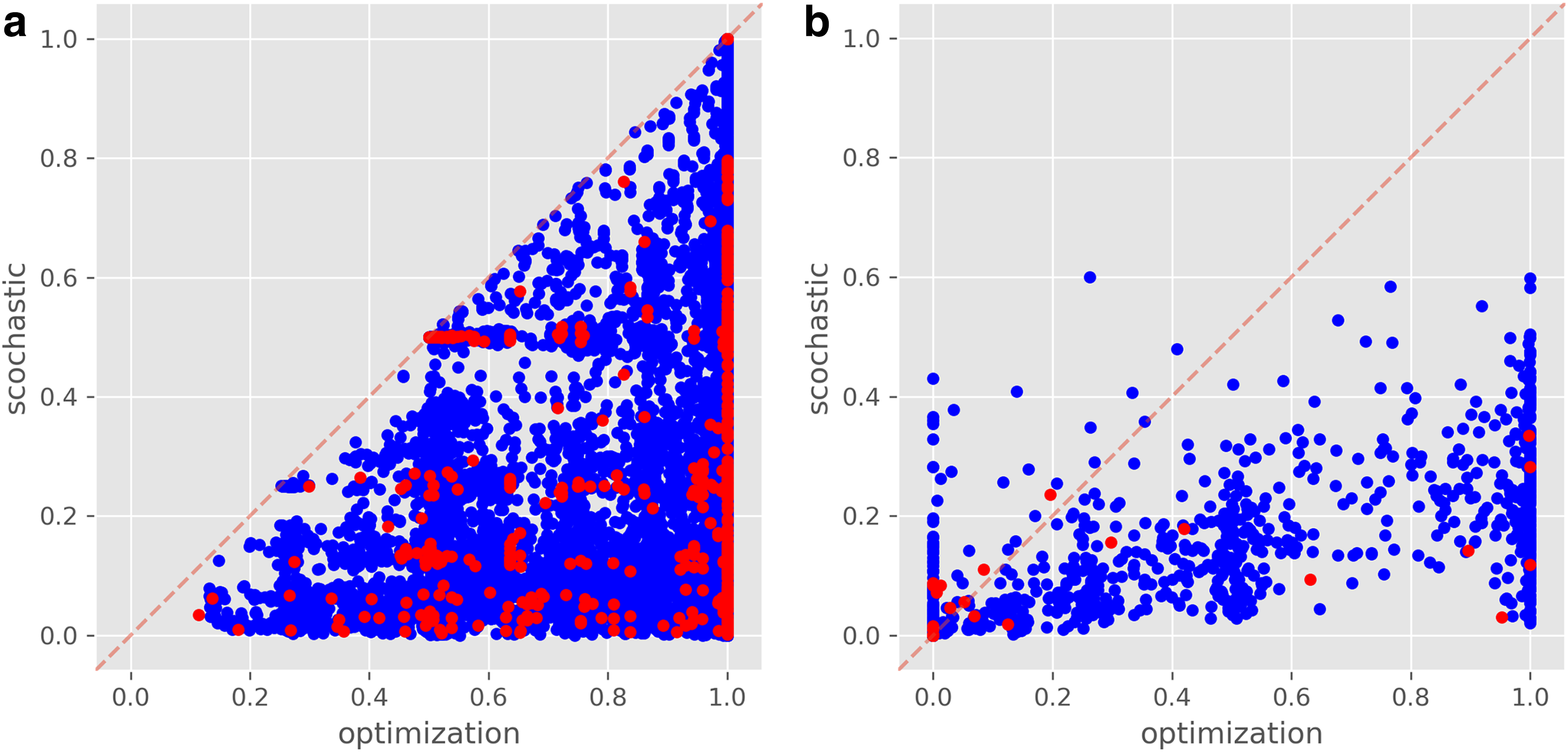
It is interesting to compare the stochastic scores that measure the mean sensitivity to a change versus the ILP-based optimization scores that measure the extremes. As an example, The majority of models had an optimization score of 1 for attractor elimination, but less than $5 %$ of the models had the corresponding stochastic score of 1, suggesting that there is a marked difference between a random perturbation to the logic of a model and a targeted one. For individual nodes, there was a correlation of $0.20$ between the stochastic and ILP-based variants. For state perturbations, there was a strong correlation ( $0.74$ ) between the stochastic and ILP-based variants. These relationships are visualized in Figure 3. The ILP-based scores are not a perfect upper bound for the stochastic ones since they assume a restricted path length to a modified attractor, but are almost always higher for the same model.

FIG. 3.

Scatter plots comparing ILP-based and stochastic-based scores across all models. Real models appear in red and randomized models in blue. (a) Per-node model perturbation scores. (b) State perturbation scores.

5. Conclusions

We have presented a first analysis of the attractor landscape of Boolean models of cellular circuits and its sensitivity to state and logic changes. Our analysis combined novel ILP formulations with stochastic simulations to overcome the inherent complexity of the problem. We found that real models are more robust than their randomized counterparts with respect to both state and logic changes. The significant difference between real and random models, across the four measures, supports the motivating assumption that the abstract notion of robustness is captured in the dynamics of Boolean models.

While the analysis could be successfully applied to dozens of circuits with up to 62 nodes each, the optimization problem remains challenging for larger circuits, especially when allowing longer paths from a state to its associated attractor. Another interesting problem is the generalization of the methods presented to asynchronous update schemes. Finally, further research is required to gain insight into the mechanisms behind the increased robustness of real models.

Footnotes

Author Disclosure Statement

The authors declare they have no conflicting financial interests.

Funding Information

R.S. was supported by a research grant from the Israel Science Foundation (no. 715/18). A.B. was support by the Deutsch Research Fund.

References

Aldana

, and Cluzel

2003. A natural class of robust networks. Proc. Natl. Acad. Sci. U.S.A. 100, 8710–8714.

Alon

, Surette

M.G.

, Barkai

, et al. 1997. Robustness in bacterial chemotaxis. Nature, 387, 913–917.

Chaouiya

, Naldi

, and Thieffry

2012. Logical modelling of gene regulatory networks with GINsim. Methods Mol. Biol. 804, 463–479.

Chatr-Aryamontri

, Breitkreutz

B.J.

, Oughtred

, et al. 2015. The BioGRID interaction database: 2015 update. Nucleic Acids Res. 43, D470–D478.

Chaves

, Eissing

, and Allgöwer

2008. Bistable biological systems: A characterization through local compact input-to-state stability. IEEE Trans. Autom. Control, 53, 87–100.

Chen

, and Aihara

2002. Stability of genetic regulatory networks with time delay. IEEE Trans. Circuits Syst. I, 49, 602–608.

Chen

, and Aihara

2006. Piecewise-linear models of genetic regulatory networks: Equilibria and their stability. J. Math. Biol. 52, 27–56.

Cowen

, Ideker

, Raphael

B.J.

, et al. 2017. Network propagation: A universal amplifier of genetic associations. Nat. Rev. Genet. 18, 551–562.

Daniels

B.C.

, Kim

, Moore

, et al. 2018. Criticality distinguishes the ensemble of biological regulatory networks. Phys. Rev. Lett. 121, 138102.

10.

Dasika

M.S.

, Burgard

, and Maranas

C.D.

2006. A computational framework for the topological analysis and targeted disruption of signal transduction networks. Biophys. J. 91, 382–398.

11.

Dittrich

M.T.

, Klau

G.W.

, Rosenwald

, et al. 2008. Identifying functional modules in protein-protein interaction networks: An integrated exact approach. Bioinformatics, 24, i223–i231.

12.

Dubrova

, and Teslenko

2011. A SAT-based algorithm for finding attractors in synchronous boolean networks. IEEE/ACM Trans. Comput. Biol. Bioinform. 8, 1393–1399.

13.

Fretter

, Szejka

, and Drossel

2009. Perturbation propagation in random and evolved boolean networks. New J. Phys., 11, 033005:1–13.

14.

Gat-Viks

, Tanay

, Raijman

, et al. 2006. A probabilistic methodology for integrating knowledge and experiments on biological networks. J. Comput. Biol. 13, 165–181.

15.

Ghanbarnejad

, and Klemm

2012. Impact of individual nodes in boolean network dynamics. EPL Europhys. Lett. 99, 58006.

16.

Grieco

, Calzone

, Bernard-Pierrot

, et al. 2013. Integrative modelling of the influence of MAPK network on cancer cell fate decision. PLoS Comput. Biol. 9, e1003286.

17.

Helikar

, Kowal

, McClenathan

, et al. 2012. The cell collective: Toward an open and collaborative approach to systems biology. BMC Syst. Biol. 6, 96.

18.

Huang

S.S.

, and Fraenkel

2009. Integrating proteomic and transcriptional and interactome data reveals hidden components of signaling and regulatory networks. Sci. Signal, 2, ra40.

19.

Huard

, Mueller

, Gilles

E.D.

, et al. 2012. An integrative model links multiple inputs and signaling pathways to the onset of DNA synthesis in hepatocytes. FEBS J. 279, 3290–3313.

20.

Ideker

, Ozier

, Schwikowski

, et al. 2002. Discovering regulatory and signalling circuits in molecular interaction networks. Bioinformatics, 18, 1:s233–s240.

21.

Jonsson

P.F.

, and Bates

P.A.

2006. Global topological features of cancer proteins in the human interactome. Bioinformatics, 22, 2291–2297.

22.

Kauffman

S.A.

1969. Metabolic stability and epigenesis in randomly constructed genetic nets. J. Theor. Biol. 22, 437–467.

23.

Klemm

, and Bornholdt

2002. Specificity and stability in topology of protein networks. Science, 296, 910–913.

24.

Klemm

, and Bornholdt

2005. Topology of biological networks and reliability of information processing. Proc. Natl. Acad. Sci. U.S.A. 102, 18414–18419.

25.

, Long

, Lu

, et al. 2004. The yeast cellcycle network is robustly designed. Proc. Natl. Acad. Sci. U.S.A. 101, 4781–4786.

26.

Lyapunov

A.M.

2007. The general problem of the stability of motion. Int. J. Control, 55, 531–534.

27.

Mitsos

, Melas

I.N.

, Siminelakis

, et al. 2009. Identifying drug effects via pathway alterations using an integer linear programming optimization formulation on phosphoproteomic data. PLoS Comput. Biol. 5, e1000591.

28.

Moignard

, Woodhouse

, Haghverdi

, et al. 2015. Decoding the regulatory network of early blood development from single-cell gene expression measurements. Nat. Biotechnol. 33, 269–276.

29.

Morris

M.K.

, Saez-Rodriguez

, Clarke

D.C.

, et al. 2011. Training signaling pathway maps to biochemical data with constrained fuzzy logic: Quantitative analysis of liver cell responses to inflammatory stimuli. PLoS Comput. Biol. 7, e1001099.

30.

Morris

M.K.

, Saez-Rodriguez

, Sorger

P.K.

, et al. 2010. Logic-based models for the analysis of cell signaling networks. Biochemistry, 49, 3216–3224.

31.

Novere

N.L.

2015. Quantitative and logic modelling of molecular and gene networks. Nat. Rev. Genet. 16, 146–158.

32.

Oda

, Matsuoka

, Funahashi

, et al. 2005. A comprehensive pathway map of epidermal growth factor receptor signaling. Mol. Syst. Biol. 1, 0010.

33.

Peixoto

T.P.

2010. Redundancy and error resilience in boolean networks. Phys. Rev. Lett. 104, 048701.

34.

Qiu

, Tamura

, Ching

W.K.

, et al. 2014. On control of singleton attractors in multiple boolean networks: Integer programming-based method. BMC Syst. Biol. 8 Suppl 1, S7.

35.

Saez-Rodriguez

, Alexopoulos

L.G.

, Epperlein

, et al. 2009. Discrete logic modelling as a means to link protein signalling networks with functional analysis of mammalian signal transduction. Mol. Syst. Biol. 5, 331.

36.

Said

M.R.

, Begley

T.J.

, Oppenheim

A.V.

, et al. 2004. Global network analysis of phenotypic effects: Protein networks and toxicity modulation in saccharomyces cerevisiae. Proc. Natl. Acad. Sci. U.S.A. 101, 18006–18011.

37.

Samaga

, Saez-Rodriguez

, Alexopoulos

L.G.

, et al. 2009. The logic of EGFR/ErbB signaling: Theoretical properties and analysis of high-throughput data. PLoS Comput. Biol. 5, e1000438.

38.

Schwab

, Siegle

, Kühlwein

, et al. 2017. Stability of signaling pathways during aging—A boolean network approach. Biology, 6, 46.

39.

Sevim

, and Rikvold

P.A.

2008. Chaotic gene regulatory networks can be robust against mutations and noise. J. Theor. Biol. 253, 323–332.

40.

Shachar

, Ungar

, Kupiec

, et al. 2008. A systems-level approach to mapping the telomere length maintenance gene circuitry. Mol. Syst. Biol. 4, 172.

41.

Sharan

, and Karp

R.M.

2006. Reconstructing boolean models of signaling. J. Comput. Biol. 13, 165–181.

42.

Silberberg

, Kupiec

, and Sharan

2014. A method for predicting protein-protein interaction types. PLoS One, 9, e90904.

43.

Vandin

, Upfal

, and Raphael

B.J.

2011. Algorithms for detecting significantly mutated pathways in cancer. J. Comput. Biol. 18, 507–522.

44.

Vardi

, Ruppin

, and Sharan

2012. A linearized constraint-based approach for modeling signaling networks. J. Comput. Biol. 19, 232–240.

45.

Yeger-Lotem

, Riva

, Su

L.J.

, et al. 2009. Bridging high-throughput genetic and transcriptional data reveals cellular responses to alpha-synuclein toxicity. Nat. Genet. 41, 316–323.

46.

Yosef

, Ungar

, Zalckvar

, et al. 2009. Toward accurate reconstruction of functional protein networks. Mol. Syst. Biol. 5, 248.