Sorting by Genome Rearrangements on Both Gene Order and Intergenic Sizes

Abstract

During the evolutionary process, genomes are affected by various genome rearrangements, that is, events that modify large stretches of the genetic material. In the literature, a large number of models have been proposed to estimate the number of events that occurred during evolution; most of them represent a genome as an ordered sequence of genes, and, in particular, disregard the genetic material between consecutive genes. However, recent studies showed that taking into account the genetic material between consecutive genes can enhance evolutionary distance estimations. Reversal and transposition are genome rearrangements that have been widely studied in the literature. A reversal inverts a (contiguous) segment of the genome, while a transposition swaps the positions of two consecutive segments. Genomes also undergo nonconservative events (events that alter the amount of genetic material) such as insertions and deletions, in which genetic material from intergenic regions of the genome is inserted or deleted, respectively. In this article, we study a genome rearrangement model that considers both gene order and sizes of intergenic regions. We investigate the reversal distance, and also the reversal and transposition distance between two genomes in two scenarios: with and without nonconservative events. We show that these problems are NP-hard and we present constant ratio approximation algorithms for all of them. More precisely, we provide a 4-approximation algorithm for the reversal distance, both in the conservative and nonconservative versions. For the reversal and transposition distance, we provide a 4.5-approximation algorithm, both in the conservative and nonconservative versions. We also perform experimental tests to verify the behavior of our algorithms, as well as to compare the practical and theoretical results. We finally extend our study to scenarios in which events have different costs, and we present constant ratio approximation algorithms for each scenario.

1. Introduction

Genome rearrangements are events that insert, remove, or change the position and orientation of large stretches of the genetic material of a genome. When we compare the genomes of two individuals, one of the main goals is to estimate the number of rearrangement events that transformed one genome into the other.

A model $ℳ$ determines the set of rearrangement events allowed to modify a genome. The size of the smallest sequence of rearrangement events in a model $ℳ$ capable of transforming a genome into another is called rearrangement distance. When we assume that no duplicated gene is present in a genome G, we can map each gene to a unique integer between 1 and n, and thus represent G as a permutation $π$ . Usually, rearrangement problems are treated as sorting problems, and the goal is to turn any genome (or permutation) $π$ of size n into a specific genome $ι = (1, \dots, n)$ , called identity permutation. If the orientation of the genes is known, a positive or negative sign is assigned to each element. Otherwise, signs are omitted.

A reversal in a permutation $π$ inverts a (contiguous) segment of $π$ , while a transposition swaps the positions of two consecutive segments. When the orientation of genes is unknown, it has been proved that the Sorting Permutations by Reversals problem is NP-hard (Caprara, 1999), and the best approximation algorithm has an approximation factor of 1.375 (Berman et al., 2002). The Sorting Permutations by Transpositions problem is also NP-hard (Bulteau et al., 2012), and the best approximation algorithm has an approximation factor of 1.375 (Elias and Hartman, 2006). If the model $ℳ$ allows both reversals and transpositions, the problem is called Sorting Permutations by Reversals and Transpositions. This problem is NP-hard (Oliveria et al., 2019a) and the best approximation algorithm has an approximation factor of $2.8334 + ε$ , for any $ε > 0$ (Rahman et al., 2008).

The representation of a genome as an ordered sequence of genes is very useful and broadly used; however, in that case, any information not present on genes is discarded, which results in some loss of information. In particular, intergenic regions between consecutive genes are not taken into account by these representations. Recently, it has been suggested that incorporating this information may improve the distance estimation from an evolutionary point of view (Biller et al., 2016a, 2016b). Thus, it is of interest to perform investigations considering the order of the genes and the size of the intergenic regions. Studies considering gene order and intergenic sizes have already been published. A model allowing double-cut and join (DCJ) operations has already been published: a problem wherein the model allows DCJ has been proved NP-hard, and a 4/3-approximation algorithm exists (Fertin et al., 2017). The DCJ (Yancopoulos et al., 2005) is a rearrangement event that cuts the genome into two points and the extremities of the resulting segments are reassembled following specific criteria. A model allowing DCJs, insertions, and deletions, where insertions and deletions act only on intergenic regions, has an exact polynomial time algorithm for a specific cost function that considered DCJs to be much less frequent than insertions or deletions (Bulteau et al., 2016). Besides, a model that also considers sizes of intergenic regions and allows only super short reversals (i.e., reversals that affect at most two genes) was presented (Oliveria et al., 2018).

In this article, we consider that orientations of gene are unknown. We investigate four problems that aim at computing the distance between genomes, taking into account intergenic regions. Two of these problems allow just conservative events of reversal and transposition: Sorting by Intergenic Reversals (SbIR) and Sorting by Intergenic Reversals and Transpositions (SbIRT). The other two problems allow nonconservative events of insertion and deletion within intergenic regions: Sorting by Intergenic Reversals, Insertions, and Deletions (SbIRID) and Sorting by Intergenic Reversals, Transpositions, Insertions, and Deletions (SbIRTID). For each of these four aforementioned problems, we assume that each operation (reversal, transposition, insertion, and deletion) has a unit cost—we thus call them “unweighted problems.” Furthermore, we extend our study, by considering different cost functions (i.e., weights) for each operation, and study weighted versions of SbIRT, SbIRID, and SbIRTID problems.

This article is organized as follows. Section 2 provides definitions and preliminary results that will be useful throughout the article. Section 3 presents results for unweighted problems. Section 4 shows experimental results for the unweighted problems. Section 5 investigates weighted versions of SbIRT, SbIRID, and SbIRTID for different weight functions. Section 6 concludes the article.

2. Formal Definitions

We define a genome $G$ as an ordered sequence of n genes $π_{1}, \dots, π_{n}$ , together with a sequence of $n + 1$ intergenic regions ${\overset{⌣}{π}}_{1}, \dots, {\overset{⌣}{π}}_{n + 1}$ , where each gene $π_{i}$ , $1 \leq i \leq n$ , is surrounded by the two intergenic regions ${\overset{⌣}{π}}_{i}$ and ${\overset{⌣}{π}}_{i + 1}$ , and we denote $G$ as follows: $G = ({\overset{⌣}{π}}_{1}, π_{1}, {\overset{⌣}{π}}_{2}, π_{2}, \dots, {\overset{⌣}{π}}_{n}, π_{n}, {\overset{⌣}{π}}_{n + 1}) .$ Our representation assumes that (i) orientation of genes is unknown, (ii) there are no duplicate genes, and (iii) the genomes share the same set of genes. In this way, we can assign each gene a unique integer between 1 and n, and transform the gene sequence $π_{1}, \dots, π_{n}$ into a permutation $π = (π_{1} π_{2} ... π_{n}), π_{i} ϵ ℕ, 1 \leq π_{1} \leq n, with π_{i} \neq π_{j} for all i \neq j .$

Rearrangement events can split intergenic regions, and each intergenic region has a well-defined number of nucleotides. Thus, we represent them by their sizes (number of nucleotides). We thus denote the sequence of intergenic regions $\overset{⌣}{π} = ({\overset{⌣}{π}}_{1}, {\overset{⌣}{π}}_{2} \dots, {\overset{⌣}{π}}_{n + 1})$ , where each ${\overset{⌣}{π}}_{i} \in N$ , $1 \leq i \leq n + 1$ , represents an intergenic region size, in such a way that ${\overset{⌣}{π}}_{i}$ is on the left side of $π_{i}$ , whereas ${\overset{⌣}{π}}_{i + 1}$ is on its right side. Thus, we can represent a genome $G$ by the pair $(π, \overset{⌣}{π})$ .

Since we are comparing two genomes and representing them as permutations, we can always assume that one of them is the identity permutation and label the other accordingly. Therefore, let $\overset{⌣}{π}$ be the intergenic region sizes of the genome assumed as $π$ and $\overset{⌣}{ι}$ be the intergenic region sizes of the other genome being compared, an instance of our problem is a tuple $(π, \overset{⌣}{π}, \overset{⌣}{ι})$ and the rearrangement distance considering a model $ℳ$ is denoted $d_{S} (π, \overset{⌣}{π}, \overset{⌣}{ι})$ , where $S$ denotes the initials of the sorting problem that uses $ℳ$ .

Definition 1 (Intergenic reversal). Let $i, j, x, y$ be integers such that $1 \leq i \leq j \leq n$ , $0 \leq x \leq {\overset{⌣}{π}}_{i}$ , and $0 \leq y \leq {\overset{⌣}{π}}_{j + 1}$ . An intergenic reversal $ρ_{(x, y)}^{(i, j)}$ splits the intergenic regions ${\overset{⌣}{π}}_{i}$ and ${\overset{⌣}{π}}_{j + 1}$ as follows: ${\overset{⌣}{π}}_{i} = x | x'$ with $x' = {\overset{⌣}{π}}_{i} - x$ and ${\overset{⌣}{π}}_{j + 1} = y | y'$ with $y' = {\overset{⌣}{π}}_{j + 1} - y$ , respectively. The sequence $(x', π_{i}, {\overset{⌣}{π}}_{i + 1} \dots {\overset{⌣}{π}}_{j}, π_{j}, y)$ is reversed and the pieces $x | y$ and $x' | y'$ form the new intergenic regions at positions i and $j + 1$ .

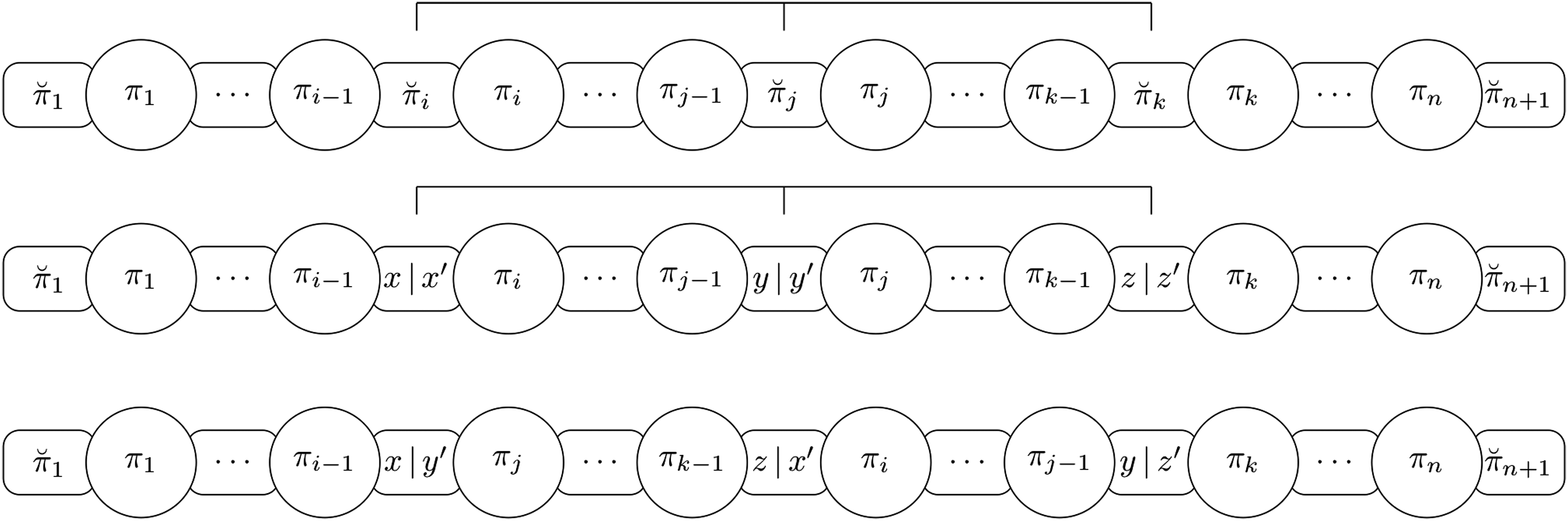
Definition 2 (Intergenic transposition). Let $i, j, k, x, y, z$ be integers such that $1 \leq i < j < k \leq n + 1$ , $0 \leq x \leq {\overset{⌣}{π}}_{i}$ , $0 \leq y \leq {\overset{⌣}{π}}_{j}$ , and $0 \leq z \leq {\overset{⌣}{π}}_{k}$ . An intergenic transposition $τ_{(x, y, z)}^{(i, j, k)}$ splits the intergenic regions ${\overset{⌣}{π}}_{i}$ , ${\overset{⌣}{π}}_{j}$ , and ${\overset{⌣}{π}}_{k}$ as follows: ${\overset{⌣}{π}}_{i} = x | x'$ with $x' = {\overset{⌣}{π}}_{i} - x$ , ${\overset{⌣}{π}}_{j} = y | y'$ with $y' = {\overset{⌣}{π}}_{j} - y$ , and ${\overset{⌣}{π}}_{k} = z | z'$ with $z' = {\overset{⌣}{π}}_{k} - z$ , respectively. The sequences $(x', π_{i}, {\overset{⌣}{π}}_{i + 1}, \dots {\overset{⌣}{π}}_{j - 1}, π_{j - 1}, y)$ and $(y', π_{j}, {\overset{⌣}{π}}_{j + 1} \dots {\overset{⌣}{π}}_{k - 1}, π_{k - 1}, z)$ swap positions without changing orientation, and pieces $x | y'$ , $z | x'$ , and $y | z'$ form the new intergenic regions at position i, $k + i - j$ , and k.

Figures 1 and 2 illustrate the notions of intergenic reversal and intergenic transposition, respectively.

FIG. 1.

Intergenic reversal as described in Definition 1.

FIG. 2.

Intergenic transposition as described in Definition 2.

Definition 3 (Intergenic insertion). Let i and x be two integers such that $1 \leq i \leq n + 1$ and $x > 0$ . An intergenic insertion $ϕ_{x}^{i}$ acts on the intergenic region ${\overset{⌣}{π}}_{i}$ by inserting x nucleotides in ${\overset{⌣}{π}}_{i}$ , resulting in a new intergenic region size of ${\overset{⌣}{π}}_{i} + x$ .

Definition 4 (Intergenic deletion). Let i and x be two integers such that $1 \leq i \leq (n + 1)$ and $0 < x \leq {\overset{⌣}{π}}_{i}$ . An intergenic deletion $ψ_{x}^{i}$ acts on the intergenic region ${\overset{⌣}{π}}_{i}$ by removing x nucleotides from ${\overset{⌣}{π}}_{i}$ , resulting in a new intergenic region size of ${\overset{⌣}{π}}_{i} - x$ .

From now on, if clear from the context, we refer to the aforementioned defined operations simply as a reversal, transposition, insertion, and deletion, respectively. Note that reversals and transpositions do not insert or delete genetic material. Thus, if a rearrangement model includes only reversals and/or transpositions, then we are dealing with conservative events, and the sums of sizes of intergenic regions in both input genomes are the same.

Given a permutation $π$ with n elements, the extended permutation of $π$ is the permutation to which two new elements are added: $π_{0} = 0$ and $π_{n + 1} = n + 1$ . From now on, we exclusively work on extended permutations, while simply calling them permutations to lighten the notations.

In the following, we often need to compare the sizes of intergenic regions in the two input genomes.

Definition 5. An intergenic region ${\overset{⌣}{π}}_{i}$ between two consecutive elements $π_{i - 1}$ and $π_{i}$ $(| π_{i} - π_{i - 1} | = 1)$ in $π$ has (in)correct size if the size of the intergenic region ${\overset{⌣}{ι}}_{k}$ is (not) the same in $ι$ , such that $ι_{k - 1} = min (π_{i - 1}, π_{i})$ and $ι_{k} = max (π_{i - 1}, π_{i})$ .

Definition 6 (Intergenic breakpoint). An intergenic breakpoint is a pair of elements $π_{i}$ and $π_{i + 1}$ from permutation $π$ , $0 \leq i \leq n$ , such that either they are not consecutive in the identity permutation $ι$ or they are consecutive but the intergenic region ${\overset{⌣}{π}}_{i + 1}$ is of incorrect size.

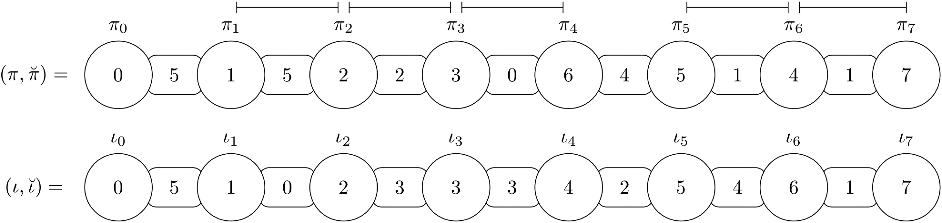
An intergenic breakpoint thus represents a region that at some point needs to be affected by some operation, either to fix the gene order or the size of the intergenic region. Figure 3 shows examples of intergenic breakpoints. The total number of intergenic breakpoints in an instance $(π, \overset{⌣}{π}, \overset{⌣}{ι})$ is denoted as $i b (π, \overset{⌣}{π}, \overset{⌣}{ι})$ .

FIG. 3.

Intergenic breakpoints for the instance $(π, \overset{⌣}{π}, \overset{⌣}{ι})$ with $π = (0, 1, 2, 3, 6, 5, 4, 7)$ , $\overset{⌣}{π} = (5, 5, 2, 0, 4, 1, 1)$ , and $\overset{⌣}{ι} = (5, 0, 3, 3, 2, 4, 1)$ are the following: $(π_{1}, π_{2})$ , $(π_{2}, π_{3})$ , $(π_{3}, π_{4})$ $(π_{5}, π_{6})$ , and $(π_{6}, π_{7})$ , as symbolized by the line segments above the figure. The elements of the intergenic breakpoints $(π_{3}, π_{4})$ and $(π_{6}, π_{7})$ are not consecutive in $ι$ , while the elements of the intergenic breakpoints $(π_{1}, π_{2})$ , $(π_{2}, π_{3})$ , and $(π_{5}, π_{6})$ are, but the intergenic regions between the elements have incorrect sizes.

The following remark will also be useful for the rest of the article.

Remark 1. The instance $(ι, \overset{⌣}{ι}, \overset{⌣}{ι})$ is the only instance for which $i b (ι, \overset{⌣}{ι}, \overset{⌣}{ι}) = 0$ .

Definition 7 (Overcharged intergenic breakpoint). An intergenic breakpoint $(π_{i}, π_{i + 1})$ is said to be overcharged if $| π_{i + 1} - π_{i} | = 1$ and ${\overset{⌣}{π}}_{i + 1} > {\overset{⌣}{ι}}_{k}$ , where ${\overset{⌣}{ι}}_{k}$ is the intergenic region between the elements $π_{i}$ and $π_{i + 1}$ in the extended identity permutation $ι$ .

Definition 8 (Undercharged intergenic breakpoint). An intergenic breakpoint $(π_{i}, π_{i + 1})$ is said to be undercharged if $| π_{i + 1} - π_{i} | = 1$ and ${\overset{⌣}{π}}_{i + 1} < {\overset{⌣}{ι}}_{k}$ , where ${\overset{⌣}{ι}}_{k}$ is the intergenic region between the elements $π_{i}$ and $π_{i + 1}$ in the extended identity permutation $ι$ .

Overcharged and undercharged intergenic breakpoints thus represent a region for which the elements are already consecutive both in $π$ and $ι$ , but the sizes of intergenic regions between are not equal. More precisely, an overcharged intergenic breakpoint has more nucleotides than necessary in ${\overset{⌣}{π}}_{i + 1}$ . Oppositely, an undercharged intergenic breakpoint has fewer nucleotides than necessary in ${\overset{⌣}{π}}_{i + 1}$ . For example, as shown in Figure 3, the intergenic breakpoint $(π_{1}, π_{2})$ is overcharged, while the intergenic breakpoint $(π_{5}, π_{6})$ is undercharged.

The variation in the number of intergenic breakpoints after applying an operation X is denoted as $Δ_{i b} (π, \overset{⌣}{π}, \overset{⌣}{ι}, X)$ , and is defined as follows: $Δ_{i b} (π, \overset{⌣}{π}, \overset{⌣}{ι}, X) = i b ((π, \overset{⌣}{π}, \overset{⌣}{ι}) \cdot X) - i b (π, \overset{⌣}{π}, \overset{⌣}{ι})$ , where $(π, \overset{⌣}{π}, \overset{⌣}{ι}) \cdot X$ denotes the new instance obtained after operation X is applied to $(π, \overset{⌣}{π})$ .

Definition 9 (Block). Let $0 \leq a, b \leq n + 1$ be two integers. We say that $(a, b)$ is a block in $π$ if $| a - b | = 1$ , a and b are consecutive in $π$ , and the intergenic region between them is of correct size.

Definition 10 (Connected intergenic breakpoints). Let $0 \leq i < j \leq n$ be two integers. Two intergenic breakpoints $(π_{i}, π_{i + 1})$ and $(π_{j}, π_{j + 1})$ are said to be connected if the following two conditions are fulfilled.

At least one of the pairs $(π_{i}, π_{i + 1})$ , $(π_{j}, π_{j + 1})$ , $(π_{i}, π_{j})$ , $(π_{i}, π_{j + 1})$ , $(π_{i + 1}, π_{j})$ , or $(π_{i + 1}, π_{j + 1})$ corresponds to two consecutive elements in $ι$ that do not form a block in $π$ .

ii.

${\overset{⌣}{π}}_{i + 1} + {\overset{⌣}{π}}_{j + 1} \geq {\overset{⌣}{ι}}_{k}$ , where ${\overset{⌣}{ι}}_{k}$ is the size of the intergenic region between the pair of consecutive elements [from (i)] in $ι$ .

Connected intergenic breakpoints represent regions that have the potential to remove at least one intergenic breakpoint, by putting two consecutive elements side by side with the same size of intergenic region between them as in $\overset{⌣}{ι}$ . For example, as shown in Figure 3, intergenic breakpoints $(π_{3}, π_{4})$ and $(π_{6}, π_{7})$ are connected, since the pair $(π_{4}, π_{7})$ corresponds to two consecutive elements in $ι$ and ${\overset{⌣}{π}}_{4} + {\overset{⌣}{π}}_{7} \geq {\overset{⌣}{ι}}_{7}$ , while intergenic breakpoints $(π_{2}, π_{3})$ and $(π_{3}, π_{4})$ are not.

Now we present a series of lower bounds for the problems studied in this article.

Lemma 1. $Δ_{i b} (π, \overset{⌣}{π}, \overset{⌣}{ι}, ρ) \geq - 2$ for any reversal $ρ$ .

Proof. Since any reversal affects only two pairs of elements and two intergenic regions, it is impossible to remove more than two intergenic breakpoints.

Lemma 2. $Δ_{i b} (π, \overset{⌣}{π}, \overset{⌣}{ι}, τ) \geq - 3$ for any transposition $τ$ .

Proof. Since any transposition affects only three pairs of elements and three intergenic regions, it is impossible to remove more than three intergenic breakpoints.

Lemma 3. $Δ_{i b} (π, \overset{⌣}{π}, \overset{⌣}{ι}, ϕ) \geq - 1$ for any insertion $ϕ$ .

Proof. Since an insertion acts in just one intergenic region, this means that the best scenario removes an intergenic breakpoint $(π_{i - 1}, π_{i})$ after applying an insertion $ϕ_{x}^{i}$ , reducing by one the number of intergenic breakpoints.

Lemma 4. $Δ_{i b} (π, \overset{⌣}{π}, \overset{⌣}{ι}, ψ) \geq - 1$ for any deletion $ψ$ .

Proof. Since a deletion acts in just one intergenic region, this means that the best scenario removes an intergenic breakpoint $(π_{i - 1}, π_{i})$ after applying a deletion $ψ_{x}^{i}$ , reducing by one the number of intergenic breakpoints.

Proposition 5. $d_{S b I R} (π, \overset{⌣}{π}, \overset{⌣}{ι}) \geq \frac{i b (π, \overset{⌣}{π}, \overset{⌣}{ι})}{2}$ .

Proof. By Remark 1, we know that $(ι, \overset{⌣}{ι}, \overset{⌣}{ι})$ is the only instance with no intergenic breakpoints. To reach the identity permutation and to correct all the sizes of intergenic regions according to $\overset{⌣}{ι}$ , we need to remove $i b (π, \overset{⌣}{π}, \overset{⌣}{ι})$ intergenic breakpoints. Also, by Lemma 1, a reversal removes at most two intergenic breakpoints and thus the proposition follows.

Proposition 6. $d_{S b I R I D} (π, \overset{⌣}{π}, \overset{⌣}{ι}) \geq \frac{i b (π, \overset{⌣}{π}, \overset{⌣}{ι})}{2}$ .

Proof. The proof is similar to proof of Proposition 5, and is obtained by Remark 1, Lemmas 1, 3, and 4.

Proposition 7. $d_{S b I R T} (π, \overset{⌣}{π}, \overset{⌣}{ι}) \geq \frac{i b (π, \overset{⌣}{π}, \overset{⌣}{ι})}{3}$ .

Proof. Directly by Remark 1 and Lemmas 1 and 2.

Proposition 8. $d_{S b I R T I D} (π, \overset{⌣}{π}, \overset{⌣}{ι}) \geq \frac{i b (π, \overset{⌣}{π}, \overset{⌣}{ι})}{3}$ .

Proof. Directly by Remark 1 and Lemmas 1–4.

3. Unweighted Operations

We start this section by proving that the problems SbIR, SbIRID, SbIRT, and SbIRTID are NP-hard. For each of these problems, the goal is to find the minimum number of operations that are necessary to solve a given instance $(π, \overset{⌣}{π}, \overset{⌣}{ι})$ —whereas all operations have the same weight. Our strategy is to either reduce from the Sorting by Reversals (SbR) or from the Sorting by Reversals and Transpositions (SbRT) problem, which do not consider the intergenic region. Then, we present in Sections 3.1 and 3.2 approximation algorithms for each of the four problems.

The SbR problem has been proven NP-hard (Caprara, 1999). An instance of this problem consists in a permutation $δ$ and a natural number d. The goal is to determine whether it is possible to transform $δ$ into $ι$ using at most d reversals.

Proposition 9. The SbIR problem is NP-hard.

Proof. We transform any instance of SbR into an instance of SbIR by setting $π = δ$ and $\overset{⌣}{π} = \overset{⌣}{ι} = (0, 0, \dots, 0)$ . It can be seen that it is possible to transform $δ$ into $ι$ using at most d reversals if and only if $d_{S b I R} (π, \overset{⌣}{π}, \overset{⌣}{ι}) \leq d$ .

Proposition 10. The SbIRID problem is NP-hard.

Proof. We transform any instance of SbR into an instance of SbIRID by setting $π = δ$ and $\overset{⌣}{π} = \overset{⌣}{ι} = (0, 0, \dots, 0)$ . Because $\overset{⌣}{π} = \overset{⌣}{ι} = (0, 0, \dots, 0)$ , if $d_{S b I R I D} (π, \overset{⌣}{π}, \overset{⌣}{ι}) \leq d$ , then there exists a sorting sequence for SbIRID, also of length at most d, in which no insertion or deletion is applied: take any sorting sequence, and ignore insertions and deletions in it. This sequence is also a solution to SbR that uses at most d reversals. Conversely, it can be seen that any sorting sequence for SbR in $δ$ can be used as such in $(π, \overset{⌣}{π}, \overset{⌣}{ι})$ , and thus if d reversals at most are used for SbR, then $d_{S b I R I D} (π, \overset{⌣}{π}, \overset{⌣}{ι}) \leq d$ .

The SbRT problem is also NP-hard (Oliveira et al., 2019a). Similarly to SbR, an instance of this problem consists in a permutation $δ$ and a natural number d. The goal is to determine whether it is possible to transform $δ$ into $ι$ applying at most d operations, each operation being either a reversal or a transposition.

Proposition 11. The SbIRT problem is NP-hard.

Proof. Adaptation of Proposition 9 using the SbRT problem.

Proposition 12. The SbIRTID problem is NP-hard.

Proof. Adaptation of Proposition 10 using the SbRT problem.

3.1. Approximation algorithms for SbIR and SbIRID

In this section, we present approximation algorithms for SbIR and SbIRID, both reaching an approximation factor of 4.

Lemma 13. Let $(π, \overset{⌣}{π}, \overset{⌣}{ι})$ be an instance such that $\sum_{i = 1}^{n + 1} {\overset{⌣}{π}}_{i} \geq \sum_{i = 1}^{n + 1} {\overset{⌣}{ι}}_{i}$ and $i b (π, \overset{⌣}{π}, \overset{⌣}{ι}) > 1$ . Then it is always possible to find a pair of connected intergenic breakpoints.

Proof. Since $i b (π, \overset{⌣}{π}, \overset{⌣}{ι}) > 1$ , there must exist a pair of intergenic breakpoints, by definition of ib. We have to show that at least one such pair is connected. Suppose by contradiction that there exists an instance $(π, \overset{⌣}{π}, \overset{⌣}{ι})$ , such that $\sum_{i = 1}^{n + 1} {\overset{⌣}{π}}_{i} \geq \sum_{i = 1}^{n + 1} {\overset{⌣}{ι}}_{i}$ , $i b (π, \overset{⌣}{π}, \overset{⌣}{ι}) > 1$ , and there is no pair of connected intergenic breakpoints. There are two possible cases:

For all pairs of intergenic breakpoints $(π_{i}, π_{i + 1})$ and $(π_{j}, π_{j + 1})$ , the elements $(π_{i}, π_{i + 1})$ , $(π_{j}, π_{j + 1})$ , $(π_{i}, π_{j})$ , $(π_{i}, π_{j + 1})$ , $(π_{i + 1}, π_{j})$ , and $(π_{i + 1}, π_{j + 1})$ are not consecutive in the identity permutation. However, this situation cannot happen since $π$ is a permutation.

For all pairs of intergenic breakpoints $(π_{i}, π_{i + 1})$ and $(π_{j}, π_{j + 1})$ , we do not have enough intergenic material to remove any intergenic breakpoint, that is, ${\overset{⌣}{π}}_{i + 1} + {\overset{⌣}{π}}_{j + 1} < {\overset{⌣}{ι}}_{k}$ where ${\overset{⌣}{ι}}_{k}$ is the size of the intergenic region between the corresponding consecutive elements in the identity permutation. However, if this is true, then it implies that $\sum_{i = 1}^{n + 1} {\overset{⌣}{π}}_{i} < \sum_{i = 1}^{n + 1} {\overset{⌣}{ι}}_{i}$ , which contradicts the initial assumption.

Lemma 14. Let $(π_{i}, π_{i + 1})$ and $(π_{j}, π_{j + 1})$ be connected intergenic breakpoints. It is possible to remove at least one intergenic breakpoint using at most two reversals.

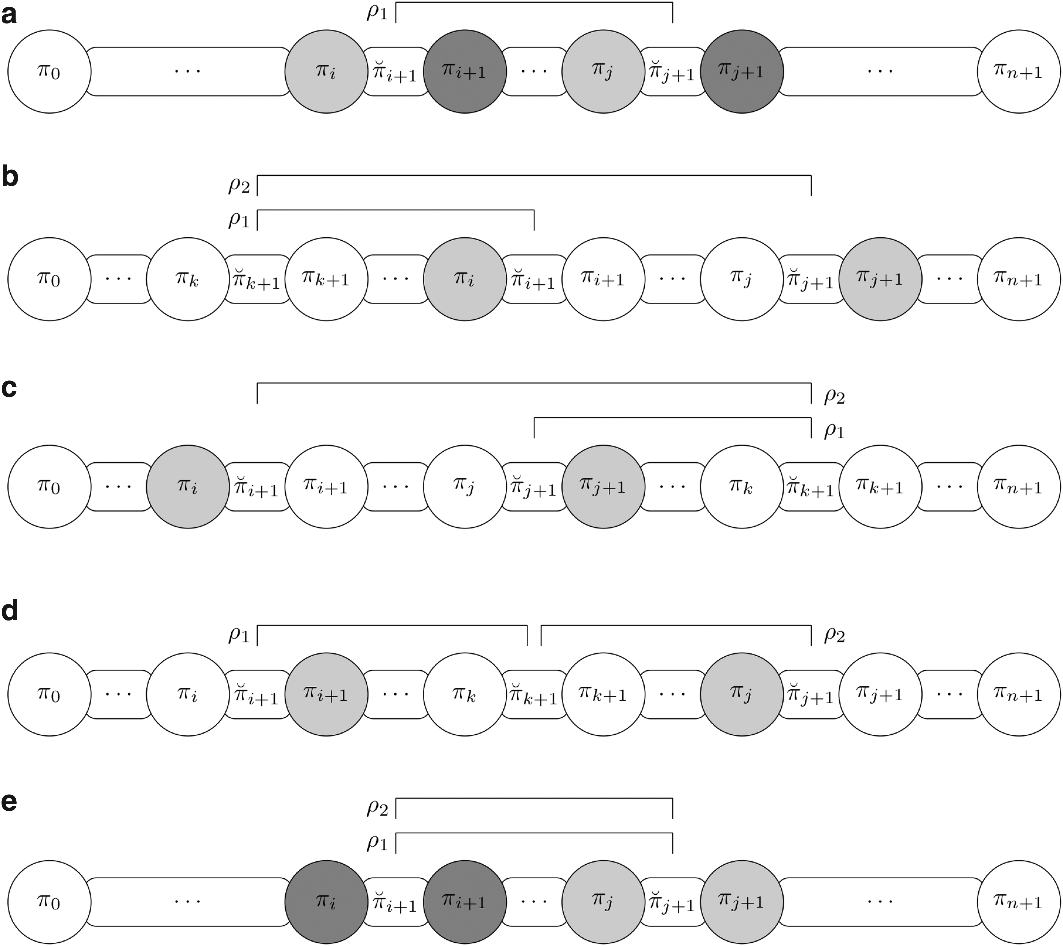
Proof. Suppose $(π_{i}, π_{i + 1})$ and $(π_{j}, π_{j + 1})$ are connected intergenic breakpoints. By definition, the following possibilities occur (see also Fig. 4 for an illustration):

FIG. 4.

The possibilities that can arise when a pair of connected intergenic breakpoints exist, and the reversals that can be applied to remove at least one intergenic breakpoint. The pair of elements that are consecutive in the identity permutation is represented with a grayscale.

$(π_{i}, π_{j})$ or $(π_{i + 1}, π_{j + 1})$ are consecutive in the identity permutation: these cases are symmetric, and we need to apply only one reversal $ρ_{(x, y)}^{(i + 1, j)}$ to place $π_{j}$ to the right of $π_{i}$ , or $π_{i + 1}$ to the left of $π_{j + 1}$ . As ${\overset{⌣}{π}}_{i + 1} + {\overset{⌣}{π}}_{j + 1} \geq {\overset{⌣}{ι}}_{k}$ , then the x and y parameters can always be chosen properly to fill the intergenic region with the correct size between the consecutive elements generated (Fig. 4a).

ii.

The pair $(π_{i}, π_{j + 1})$ is consecutive in $ι$ : in this case, we apply two consecutive reversals. In this scenario, we look for an intergenic breakpoint $(π_{k}, π_{k + 1})$ , such that $k < i$ or $k > j$ , to apply the sequence of reversals without creating new intergenic breakpoints. Let us prove, by contradiction, that such an intergenic breakpoint exists. Suppose that there is no intergenic breakpoint $(π_{k}, π_{k + 1})$ such that $k < i$ or $k > j$ . This means that the segments $(π_{0}, \dots, π_{i})$ and $(π_{j + 1}, \dots, π_{n + 1})$ are composed of consecutive elements with no intergenic breakpoint between them; we also know that $π_{i}$ and $π_{j + 1}$ are consecutive elements in $ι$ , but if both statements are true, this implies that there are no valid values for the elements $π_{i + 1}$ and $π_{j}$ of permutation $π$ . If $k < i$ , we apply the reversal $ρ_{(0, {\overset{⌣}{π}}_{i + 1})}^{(k + 1, i)}$ to reach case $(i)$ (Fig. 4b). If $k > j$ , we apply the reversal $ρ_{(0, {\overset{⌣}{π}}_{k + 1})}^{(j + 1, k)}$ to reach case $(i)$ (Fig. 4c). Note that, in both scenarios, the sizes of intergenic regions remain the same and case $(i)$ can be applied.

iii.

The pair $(π_{i + 1}, π_{j})$ is consecutive in $ι$ : in this case we apply two consecutive reversals. In this scenario, we look for an intergenic breakpoint $(π_{k}, π_{k + 1})$ , such that $k > i$ and $k < j$ , to apply the sequence of reversals without creating new intergenic breakpoints. Let us prove, by contradiction, that such an intergenic breakpoint exists. Suppose that there is no intergenic breakpoint $(π_{k}, π_{k + 1})$ such that $k > i$ and $k < j$ . This means that the segment $(π_{i + 1}, \dots, π_{j})$ is composed of consecutive elements with no intergenic breakpoint between them; we also know that $(π_{i + 1}, π_{j})$ are consecutive elements, but if both statements are true, this implies that there are no valid values for the elements $π_{i + 1}$ and $π_{j}$ of permutation $π$ . After identifying the intergenic breakpoint $(π_{k}, π_{k + 1})$ , we apply the reversal $ρ_{(0, {\overset{⌣}{π}}_{k + 1})}^{(i + 1, k)}$ (Fig. 4d) to reach case $(i)$ .

iv.

The pair $(π_{i}, π_{i + 1})$ or the pair $(π_{j}, π_{j + 1})$ is consecutive in $ι$ : these cases are symmetric and we need to apply two consecutive reversals. Initially, we apply the reversal $ρ_{(0, {\overset{⌣}{π}}_{j + 1})}^{(i + 1, j)}$ without changing the sizes of intergenic regions, as a result we reach case $(i)$ (Fig. 4e).

Theorem 15. The SbIR problem is 4-approximable.

Proof. Although the permutation is not sorted and it has intergenic regions with incorrect size, it is always possible to remove at least one intergenic breakpoint after applying at most two reversals (Lemmas 13 and 14). In the worst case, this gives us a total of $2 \cdot i b (π, \overset{⌣}{π}, \overset{⌣}{ι})$ reversals to transform $(π, \overset{⌣}{π})$ into $(ι, \overset{⌣}{ι})$ . By Proposition 5, we know that at least $i b (π, \overset{⌣}{π}, \overset{⌣}{ι}) ∕ 2$ reversals are necessary, and the theorem follows.

Lemma 16. Let $(π, \overset{⌣}{π}, \overset{⌣}{ι})$ be an instance of the SbIRID problem such that $i b (π, \overset{⌣}{π}, \overset{⌣}{ι}) > 0$ . Then it is always possible to find an insertion $ϕ$ such that $Δ_{i b} (π, \overset{⌣}{π}, \overset{⌣}{ι}, ϕ) \leq 0$ .

Proof. Since $i b (π, \overset{⌣}{π}, \overset{⌣}{ι}) > 0$ , then there exists at least one intergenic breakpoint, to which we can apply an insertion without increasing the number of intergenic breakpoints.

Lemma 17. Let $(π, \overset{⌣}{π}, \overset{⌣}{ι})$ be an instance of the SbIRID problem such that $i b (π, \overset{⌣}{π}, \overset{⌣}{ι}) = 1$ and $\sum_{i = 1}^{n + 1} {\overset{⌣}{π}}_{i} > \sum_{i = 1}^{n + 1} {\overset{⌣}{ι}}_{i}$ . Then it is always possible to find a deletion $ψ$ such that $Δ_{i b} (π, \overset{⌣}{π}, \overset{⌣}{ι}, ψ) = - 1$ .

Proof. Since $i b (π, \overset{⌣}{π}, \overset{⌣}{ι}) = 1$ , then we know that $π = ι$ , otherwise the number of intergenic breakpoints would be strictly >1. Since all the elements in $π$ are consecutive and $\sum_{i = 1}^{n + 1} {\overset{⌣}{π}}_{i} > \sum_{i = 1}^{n + 1} {\overset{⌣}{ι}}_{i}$ , there is necessarily an intergenic region ${\overset{⌣}{π}}_{k}$ such that ${\overset{⌣}{π}}_{k} > {\overset{⌣}{ι}}_{k}$ . Thus the deletion $ψ_{{\overset{⌣}{π}}_{k} - {\overset{⌣}{ι}}_{k}}^{k}$ removes the intergenic breakpoint $(π_{k - 1}, π_{k})$ and the lemma follows.

Theorem 18. The SbIRID problem is 4-approximable.

Proof. Let $(π, \overset{⌣}{π}, \overset{⌣}{ι})$ be an instance of the SbIRID problem. We are going to divide the proof into three cases, depending on the total length of intergenic regions in $π$ .

$\sum_{i = 1}^{n + 1} {\overset{⌣}{π}}_{i} > \sum_{i = 1}^{n + 1} {\overset{⌣}{ι}}_{i}$ : Lemmas 13 and 14 remain valid as long as $i b (π, \overset{⌣}{π}, \overset{⌣}{ι}) > 1$ , and we apply each time two reversals to remove an intergenic breakpoint, until we reach a permutation $μ$ such that $i b (μ, \overset{⌣}{π}, \overset{⌣}{ι}) = 1$ . Then we invoke Lemma 17 and apply one deletion to remove the last intergenic breakpoint.

ii.

$\sum_{i = 1}^{n + 1} {\overset{⌣}{π}}_{i} = \sum_{i = 1}^{n + 1} {\overset{⌣}{ι}}_{i}$ : Lemmas 13 and 14 are sufficient to sort the permutation and to fix the sizes of the intergenic regions by applying only reversals.

iii.

$\sum_{i = 1}^{n + 1} {\overset{⌣}{π}}_{i} < \sum_{i = 1}^{n + 1} {\overset{⌣}{ι}}_{i}$ : Initially we apply an insertion, so that we obtain $\sum_{i = 1}^{n + 1} {\overset{⌣}{π}}_{i} = \sum_{i = 1}^{n + 1} {\overset{⌣}{ι}}_{i}$ —we know from Lemma 16 that this is always feasible without increasing the number of breakpoints. Then, Lemmas 13 and 14 guarantee that the permutation can be sorted, and the sizes of the intergenic regions can be fixed, by applying only reversals. Note that the initial insertion may not remove any intergenic breakpoint, but then only reversals are applied. As every instance $(π, \overset{⌣}{π}, \overset{⌣}{ι})$ , which $\sum_{i = 1}^{n + 1} {\overset{⌣}{π}}_{i} = \sum_{i = 1}^{n + 1} {\overset{⌣}{ι}}_{i}$ , it is impossible to have $i b (π, \overset{⌣}{π}, \overset{⌣}{ι}) = 1$ , then the last reversal necessarily removes two intergenic breakpoints. Thus, considering the first insertion and the last reversal only, on average, it takes two operations to remove two intergenic breakpoints.

Considering the three mentioned cases, it can be seen that we need a total of at most $2 \cdot i b (π, \overset{⌣}{π}, \overset{⌣}{ι})$ operations to transform $(π, \overset{⌣}{π})$ into $(ι, \overset{⌣}{ι})$ . Since Proposition 6 yields that at least $i b (π, \overset{⌣}{π}, \overset{⌣}{ι}) ∕ 2$ operations are needed, the theorem follows.

3.2. Approximation algorithms for SbIRT and SbIRTID

In this section, we present approximation algorithms for SbIRT and SbIRTID, which both reach a factor of 4.5. We first prove in Lemma 19 an important property, which will be very helpful to design our approximation algorithms.

Lemma 19. Given two consecutive transpositions in the format: $(π, \overset{⌣}{π}) \cdot τ_{(φ_{i}, φ_{j}, φ_{k})}^{(i, j, k)} \cdot τ_{({φ'}_{i}, {φ'}_{i + k - j}, {φ'}_{k})}^{(i, i + k - j, k)} .$

It is possible to perform any redistribution of nucleotides within intergenic regions ${\overset{⌣}{π}}_{i}$ , ${\overset{⌣}{π}}_{j}$ , and ${\overset{⌣}{π}}_{k}$ .

Proof. We have to show that it is always possible to find values for the triples $(φ_{i}, φ_{j}, φ_{k})$ and $(φ_{i}', φ'_{i + k - j}, φ_{k}')$ for any redistribution of nucleotides within intergenic regions ${\overset{⌣}{π}}_{i}$ , ${\overset{⌣}{π}}_{j}$ , and ${\overset{⌣}{π}}_{k}$ .

Since we use transpositions only, we know that ${\overset{⌣}{π}}_{i} + {\overset{⌣}{π}}_{j} + {\overset{⌣}{π}}_{k} = {\overset{⌣}{π}}_{i}'' + {\overset{⌣}{π}}_{j}'' + {\overset{⌣}{π}}_{k}''$ , where ${\overset{⌣}{π}}_{i}''$ , ${\overset{⌣}{π}}_{j}''$ , and ${\overset{⌣}{π}}_{k}''$ represent the sizes of intergenic regions after applying the two consecutive transpositions.

Based on the nucleotide flow between the intergenic regions, we perform a reduction to an instance $I_{M F}$ of the maximum flow problem, and we show that it is always possible to find a solution for this instance that satisfies the redistribution constraints of the intergenic regions ${\overset{⌣}{π}}_{i}$ , ${\overset{⌣}{π}}_{j}$ , and ${\overset{⌣}{π}}_{k}$ .

Figure 5 (left) shows the flow that nucleotides within intergenic regions can follow when applying the two consecutive transpositions from the statement of Lemma 19. Note that each intergenic region can “send” nucleotides to two distinct intergenic regions. We thus can create a graph, where each vertex corresponds to an intergenic region, and where there is an arc $(i, j)$ with unlimited capacity if the intergenic region i can send nucleotides to the intergenic region j.

FIG. 5.

On the left side, a representation of the flow of nucleotides between the intergenic regions. On the right side, the instance $I_{M F}$ of the maximum flow problem with the source (0) and target (10) vertices.

Finally, to get the instance $I_{M F}$ of the maximum flow problem, we add vertices 0 (source) and 10 (target), together with the following arcs: $(0, 1)$ , $(0, 2)$ , $(0, 3)$ , $(7, 10)$ , $(8, 10)$ , and $(9, 10)$ with their respective capacities $a = {\overset{⌣}{π}}_{i}$ , $b = {\overset{⌣}{π}}_{j}$ , $c = {\overset{⌣}{π}}_{k}$ , $x = {\overset{⌣}{π}}_{i}''$ , $y = {\overset{⌣}{π}}_{j}''$ ,and $z = {\overset{⌣}{π}}_{k}''$ . All other arcs are assigned infinite capacity. Figure 5 (right) shows the instance $I_{M F}$ of the maximum flow problem that was obtained.

If we analyze Figure 5 (right), we can see that the maximum flow for instance $I_{M F}$ is limited to $max {(a + b + c), (x + y + z)}$ , but we know that $(a + b + c) = (x + y + z) = F$ . Also note that if there is a redistribution of the intergenic regions ${\overset{⌣}{π}}_{i}$ , ${\overset{⌣}{π}}_{j}$ , and ${\overset{⌣}{π}}_{k}$ , this means that the instance $I_{M F}$ has a solution where the maximum flow is F. Conversely, we can see that if the instance $I_{M F}$ has a solution with maximum flow of F and all the variables in the solution are integers, then this means that it is possible to redistribute the intergenic regions ${\overset{⌣}{π}}_{i}$ , ${\overset{⌣}{π}}_{j}$ , and ${\overset{⌣}{π}}_{k}$ .

Now, we show that the instance $I_{M F}$ always has a solution with a maximum flow F, in which all variables in the solution are integers. We prove this result by providing a solution for the instance $I_{M F}$ , which is obtained in three steps.

Step 1 consists in removing vertices 8 and 9 from $I_{M F}$ [Fig. 6 (left)], and solving the instance using linear programming to obtain a possible fractional solution. Notice that the maximum flow for this step is less or equal to x, since $(a + b + c) \geq x$ . In addition, there exists a solution that reaches exactly x (e.g., send a through the path $(1, 4, 7)$ , send b through the path $(2, 4, 7)$ , and send c through the path $(3, 5, 7)$ ). Let $X'$ be the solution matrix, in which $X'_{i, j}$ represents the flow going from vertex i to vertex j in the solution. We know that $(X'_{0, 1} + X'_{0, 2} + X'_{0, 3}) = x$ and $x \in N$ . If ${X'_{0, 1}, X'_{0, 2}, X'_{0, 3}} ⁄ \subset N$ , we can obtain integer values for the variables $X'_{0, 1}$ , $X'_{0, 2}$ , and $X'_{0, 3}$ by redistributing the fractional part between the arcs, this is possible because we know that $(a + b + c) \geq x$ . Since all paths that leave from vertices 1, 2, and 3 and reach vertex 7 have unlimited capacity, we can obtain an integer solution for the remaining variables. After this process, we obtain an integer solution $X'$ for Step 1.

FIG. 6.

Instance $I_{M F}$ divided into three steps.

Step 2 consists in removing vertices 7 and 9 from $I_{M F}$ , and updating the capacity of arcs $(0, 1)$ , $(0, 2)$ , and $(0, 3)$ to $a' = a - X'_{0, 1}$ , $b' = b - X'_{0, 2}$ , and $c' = c - X'_{0, 3}$ , respectively [Fig. 6 (center)]. In other words, we take into account, for arcs $(0, 1)$ , $(0, 2)$ , and $(0, 3)$ , the capacities that were already used in Step 1. Note that $a' + b' + c' = a + b + c - x$ , but we also know that $a + b + c = x + y + z$ , thus $a' + b' + c' = a + b + c - x = y + z \geq y$ . Note that the maximum flow for this step is ≤ y, since $a' + b' + c' \geq y$ , and there exists a solution that reaches exactly y [e.g., send $a'$ through the path $(1, 4, 8)$ , send $b'$ through the path $(2, 4, 8)$ , and send $c'$ through the path $(3, 6, 8)$ ]. Similarly to the process performed in Step 1, we solved the problem to get a solution $X''$ where the maximum flow is y and all variables are integers.

Step 3 consists in removing vertices 7 and 8 from $I_{M F}$ , and updating the capacity of arcs $(0, 1)$ , $(0, 2)$ , and $(0, 3)$ to $a'' = a' - X''_{0, 1}$ , $b'' = b' - X''_{0, 2}$ , and $c'' = c' - X''_{0, 3}$ , respectively [Fig. 6 (right)]. In other words, we take into account, for arcs $(0, 1)$ , $(0, 2)$ , and $(0, 3)$ , the capacities that were already used in steps 1 and 2. Note that $a'' + b'' + c'' = a + b + c - x - y$ , but we also know that $a + b + c = x + y + z$ , thus $a'' + b'' + c'' = a + b + c - x - y = z$ . Note that the maximum flow for this step is equal to z, since $a'' + b'' + c'' = z$ , and there exists a solution that reaches exactly z [e.g., send $a''$ through the path $(1, 5, 9)$ , send $b''$ through the path $(2, 6, 9)$ , and send $c''$ through the path $(3, 6, 9)$ ]. Similarly to the process performed in Step 1, we solve the problem to get a solution $X'''$ where the maximum flow is z and all the variables are integers.

The final solution X consists in the sum of all the capacities used by the solutions in Steps 1, 2, and 3, that is, $\forall$ $1 \leq i, j \leq 10$ , $X_{i, j} = X'_{i, j} + X''_{i, j} + X'''_{i, j}$ . Note that the solution X does not violate any capacity constraints, all variables are integers and the maximum flow is $F = a + b + c = x + y + z$ .

In summary, Lemma 19 allows us, in two transpositions, to redistribute the size of the three involved intergenic regions in any way we want, while keeping the genes in the same order in the permutation.

Lemma 20. Given an instance $(π, \overset{⌣}{π}, \overset{⌣}{ι})$ , such that $\sum_{i = 1}^{n + 1} {\overset{⌣}{π}}_{i} = \sum_{i = 1}^{n + 1} {\overset{⌣}{ι}}_{i}$ , it is possible to turn $(π, \overset{⌣}{π})$ into $(ι, \overset{⌣}{ι})$ after applying at most $3 \cdot i b (π, \overset{⌣}{π}, \overset{⌣}{ι}) ∕ 2$ operations of reversals or transpositions.

Proof. We are now going to divide our analysis into two steps. The first step consists in removing all the overcharged intergenic breakpoints.

The number of overcharged intergenic breakpoints is strictly greater than one. In that case, let us arbitrarily choose two of them. We also know there exists at least a third intergenic breakpoint b. By Lemma 19, we can, in two consecutive transpositions, move the extra intergenic material from the two overcharged intergenic breakpoints toward b, without modifying the permutation order. In that case, we have decreased the number of intergenic breakpoints by two.

The number of overcharged intergenic breakpoints is exactly one and there is an undercharged intergenic breakpoint u, such that the extra intergenic material of the overcharged intergenic breakpoint is sufficient to fill the intergenic region of u with the necessary number of nucleotides. Let o be the overcharged intergenic breakpoint. If the instance has only two intergenic breakpoints (o and u), this means that the extra intergenic material of o is the exact amount to fill the u intergenic region with the correct number of nucleotides. We can select a third intergenic region that will not be changed and by Lemma 19, we can, in two consecutive transpositions, move the extra intergenic material from o toward u, without modifying the permutation order. Otherwise, we select the third intergenic breakpoint b and by Lemma 19, we can, in two consecutive transpositions, move the extra intergenic material from o filling the intergenic region of u with the correct number of nucleotides and depositing the remaining in b, without modifying the permutation order. In that case, we have decreased the number of intergenic breakpoints by two.

The number of overcharged intergenic breakpoints is exactly one and there is not an undercharged intergenic breakpoint u, such that the extra intergenic material of the overcharged intergenic breakpoint is sufficient to fill the intergenic region of u with the necessary number of nucleotides. We know there exists at least a second intergenic breakpoint b and we can, in two consecutive reversals, move the extra intergenic material from the overcharged intergenic breakpoint toward b, without modifying the permutation order. In that case, we have decreased the number of intergenic breakpoints by one.

The worst case of this first step removes one intergenic breakpoint after applying two consecutive reversals, but if this case happens, it will be performed just once before removing all overcharged intergenic breakpoints of the instance. Note that if the first step performs the worst case, we can conclude that $(ι, \overset{⌣}{ι})$ was not reached yet, since the last transposition before transforming any genome $(π, \overset{⌣}{π})$ into $(ι, \overset{⌣}{ι})$ always removes at least two intergenic breakpoints.

The second step removes the remaining intergenic breakpoints and guarantees that no overcharged intergenic breakpoint will be created after applying a sequence of operations.

By Lemma 13, we can find at least one pair of connected intergenic breakpoints until turning $(π, \overset{⌣}{π})$ into $(ι, \overset{⌣}{ι})$ . Analyzing the possibilities to remove an intergenic breakpoint based on a pair of connected intergenic breakpoints, we have:

$(π_{i}, π_{j})$ or $(π_{i + 1}, π_{j + 1})$ : We need to apply only one reversal, which is exactly as the procedure shown in case (i) of Lemma 14. To ensure that no overcharged breakpoint has been created, we perform the first step.

ii.

$(π_{i}, π_{j + 1})$ : In this case we need to apply one transposition. As shown previously in case (ii) of Lemma 14, we know that there must exist another intergenic breakpoint $(π_{k}, π_{k + 1})$ such that $k < i$ or $k > j$ . If $k < i$ we apply a transposition $τ_{(x, y, z)}^{(k + 1, i + 1, j + 1)}$ to place the element $π_{i}$ on the left side of the element $π_{j + 1}$ (Fig. 7a). If $k > j$ we apply a transposition $τ_{(x, y, z)}^{(i + 1, j + 1, k + 1)}$ to place the element $π_{j + 1}$ on the right side of the element $π_{i}$ (Fig. 7b). In both scenarios, we have that ${\overset{⌣}{π}}_{i + 1} + {\overset{⌣}{π}}_{j + 1} \geq {\overset{⌣}{ι}}_{k}$ , then the x, y, and z parameters can always be chosen properly to fill the intergenic region with the correct size between the consecutive elements generated. To ensure that no overcharged breakpoint has been created, we perform the first step.

iii.

$(π_{i + 1}, π_{j})$ : In this case we need to apply one transposition. As shown previously in case (iii) of Lemma 14, we know that there must exist another intergenic breakpoint $(π_{k}, π_{k + 1})$ such that $k > i$ and $k < j$ . After identifying the intergenic breakpoint $(π_{k}, π_{k + 1})$ , we apply a transposition $τ_{(x, y, z)}^{(i + 1, k + 1, j + 1)}$ to place the element $π_{j}$ on the left side of the element $π_{i + 1}$ (Fig. 7c). Since ${\overset{⌣}{π}}_{i + 1} + {\overset{⌣}{π}}_{j + 1} \geq {\overset{⌣}{ι}}_{k}$ , then the x, y, and z parameters can always be chosen properly to fill the intergenic region with the correct size between the consecutive elements generated. To ensure that no overcharged breakpoint has been created, we perform the first step.

iv.

$(π_{i}, π_{i + 1})$ or $(π_{j}, π_{j + 1})$ : Note that this case will be automatically handled by cases (i), (ii), and (iii), since we removed all the overcharged intergenic breakpoints and we guarantee that none will be created.

FIG. 7.

The possibilities to remove at least one intergenic breakpoint by applying only one transposition. The pair of elements that are consecutive in the identity permutation is represented with a grayscale.

Note that all cases of the second step initially apply one operation that removes at least one intergenic breakpoint. It implies that if the first step performs the worst case, then it will necessarily be followed by one operation that removes at least one intergenic breakpoint and the lemma follows.

Theorem 21. The SbIRT problem is 4.5-approximable.

Proof. Lemma 20 shows that it is possible to transform $(π, \overset{⌣}{π}, \overset{⌣}{ι})$ into $(ι, \overset{⌣}{ι}, \overset{⌣}{ι})$ using at most $3 \cdot i b (π, \overset{⌣}{π}, \overset{⌣}{ι}) ∕ 2$ operations. By Proposition 7, we know the lower bound is $i b (π, \overset{⌣}{π}, \overset{⌣}{ι}) ∕ 3$ , and the theorem follows.

Remark 2. Considering the SbIRTID problem, note that from a sequence of rearrangement events that transforms $(α, bolditalopenαbolditalclose⌣)$ into $(σ, bolditalopenσbolditalclose⌣)$ , it is possible to obtain a sequence with the same size that transforms $(σ, bolditalopenσbolditalclose⌣)$ into $(α, bolditalopenαbolditalclose⌣)$ . For this purpose, each operation is mapped with an inverse behavior, this way:

• A deletion is mapped into an insertion.

• An insertion is mapped into a deletion.

Reversals and Transposition have the parameters modified to reflect the inverse behavior.

For this reason, we can assume for every instance $(π, \overset{⌣}{π}, \overset{⌣}{ι})$ of SbIRTID problem that $\sum_{i = 1}^{n + 1} {\overset{⌣}{π}}_{i} \leq \sum_{i = 1}^{n + 1} {\overset{⌣}{ι}}_{i}$ , since we can always choose the representation of the genome with the smallest number of nucleotides as the source genome.

Theorem 22. The SbIRTID problem is 4.5-approximable.

Proof. Let $(π, \overset{⌣}{π}, \overset{⌣}{ι})$ be an instance of the SbIRTID problem. By Remark 2, we can assume for every instance $(π, \overset{⌣}{π}, \overset{⌣}{ι})$ that $\sum_{i = 1}^{n + 1} {\overset{⌣}{π}}_{i} \leq \sum_{i = 1}^{n + 1} {\overset{⌣}{ι}}_{i}$ . We divide the proof into two cases, depending on the total length of intergenic regions in $π$ :

$\sum_{i = 1}^{n + 1} {\overset{⌣}{π}}_{i} = \sum_{i = 1}^{n + 1} {\overset{⌣}{ι}}_{i}$ : In this case, by Lemma 20, we can solve the problem using only reversals and transpositions.

ii.

$\sum_{i = 1}^{n + 1} {\overset{⌣}{π}}_{i} < \sum_{i = 1}^{n + 1} {\overset{⌣}{ι}}_{i}$ : Initially we apply an insertion, so that we obtain $\sum_{i = 1}^{n + 1} {\overset{⌣}{π}}_{i} = \sum_{i = 1}^{n + 1} {\overset{⌣}{ι}}_{i}$ —we know from Lemma 16 that this is always feasible without increasing the number of breakpoints. Then, Lemma 20 guarantees that the permutation can be sorted, and the sizes of the intergenic regions can be fixed, by applying only reversals and transpositions. Note that the initial insertion may not remove any intergenic breakpoint, but then only reversals and transpositions are applied. As every instance $(π, \overset{⌣}{π}, \overset{⌣}{ι})$ , which $\sum_{i = 1}^{n + 1} {\overset{⌣}{π}}_{i} = \sum_{i = 1}^{n + 1} {\overset{⌣}{ι}}_{i}$ , it is impossible to have $i b (π, \overset{⌣}{π}, \overset{⌣}{ι}) = 1$ , then the last operation (reversal or transposition) necessarily removes at least two intergenic breakpoints. Thus, considering the first insertion and the last operation only (reversal or transposition), on average, it takes two operations to remove two intergenic breakpoints.

Considering the two cases mentioned, it can be seen that we need a total of at most $3 \cdot i b (π, \overset{⌣}{π}, \overset{⌣}{ι}) ∕ 2$ operations to transform $(π, \overset{⌣}{π}, \overset{⌣}{ι})$ into $(ι, \overset{⌣}{ι}, \overset{⌣}{ι})$ . Since Proposition 8 yields that at least $i b (π, \overset{⌣}{π}, \overset{⌣}{ι}) ∕ 3$ operations are needed, the theorem follows.

4. Experimental Results

In this section, we show and discuss experimental results that we have obtained on simulated data concerning the SbIR and SbIRT problems.

For the SbIR problem, we created a database with 20 sets of genomes of size 100, each set containing a total of 10,000 genomes. The sets are identified by the number of operations that were applied from the target genome $(5, 10, 15, \dots, 100)$ . The target genome was created from the sorted genes (i.e., from the identity permutation $ι$ ), and each size of the intergenic region in $\overset{⌣}{ι}$ was randomly chosen between 0 and 100. From the target genome, a fixed number of reversals (defined by the set identification) was applied randomly, generating the source genome. A random reversal means that parameters i, j, x, and y have been generated randomly within the allowed ranges. The process was repeated until filling each set with a total of 10,000 source and target genomes, totaling 200,000 source and target genomes.

Considering the SbIRT problem, we created a database adopting a similar procedure described for the SbIR problem, differing only during the step wherein random operations were applied. In this case, a random reversal or transposition was applied with a probability of 0.5 for each event.

Tables 1 and 2 show the results obtained by, respectively, our 4-approximation algorithm for the SbIR problem and our 4.5-approximation algorithm for the SbIRT problems (see Theorems 15 and 21, respectively). Column (OP) represents the number of operations applied to create the instances (i.e., each of the generated sets) and column (DEE_avg) represents the average distance estimation error. For an instance $(π, \overset{⌣}{π}, \overset{⌣}{ι})$ , the distance estimation error is calculated as follows: $\frac{| D_{a l g} - O P |}{O P}$ , such that $D_{a l g}$ is the distance estimation for the instance $(π, \overset{⌣}{π}, \overset{⌣}{ι})$ computed by our algorithms. This information shows, as a percentage, how far a solution provided by our algorithms is from OP. Columns (D_min), (D_avg), and (D_max) show the minimum, average, and maximum number of operations that were applied by our algorithm, respectively. Columns (A_min), (A_avg), and (A_max) represent the minimum, average, and maximum approximation ratio obtained, respectively. The lower bounds adopted to compute the approximation factor are from Propositions 5 and 7.

Table 1.
Experimental Results for Sorting by Intergenic Reversals Problem

SbIR 4-approximation algorithm

OP DEE_avg (%) D_min D_avg D_max A_min A_avg A_max

5 11.27 4 5.56 10 1.00 1.13 2.25

10 17.35 9 11.73 20 1.00 1.25 2.12

15 21.79 14 18.27 27 1.00 1.37 2.00

20 25.85 20 25.17 35 1.05 1.49 2.07

25 28.37 24 32.09 45 1.18 1.60 2.16

30 30.26 30 39.08 51 1.27 1.70 2.18

35 30.27 36 45.60 58 1.36 1.78 2.17

40 29.11 41 51.65 65 1.47 1.84 2.21

45 26.83 44 57.08 70 1.56 1.89 2.21

50 23.55 50 61.78 75 1.61 1.92 2.17

55 19.77 52 65.87 80 1.73 1.94 2.20

60 16.03 57 69.62 86 1.74 1.96 2.18

65 12.25 60 72.95 86 1.76 1.97 2.18

70 08.47 63 75.81 90 1.81 1.98 2.18

75 05.31 67 78.42 93 1.82 1.99 2.16

80 03.50 67 80.83 95 1.83 1.99 2.20

85 03.76 69 82.84 94 1.81 2.00 2.21

90 05.98 71 84.77 100 1.85 2.00 2.17

95 08.91 75 86.54 99 1.88 2.00 2.17

100 11.98 77 88.01 99 1.88 2.01 2.18

SbIR 4-approximation algorithm
5	11.27	4	5.56	10	1.00	1.13	2.25
10	17.35	9	11.73	20	1.00	1.25	2.12
15	21.79	14	18.27	27	1.00	1.37	2.00
20	25.85	20	25.17	35	1.05	1.49	2.07
25	28.37	24	32.09	45	1.18	1.60	2.16
30	30.26	30	39.08	51	1.27	1.70	2.18
35	30.27	36	45.60	58	1.36	1.78	2.17
40	29.11	41	51.65	65	1.47	1.84	2.21
45	26.83	44	57.08	70	1.56	1.89	2.21
50	23.55	50	61.78	75	1.61	1.92	2.17
55	19.77	52	65.87	80	1.73	1.94	2.20
60	16.03	57	69.62	86	1.74	1.96	2.18
65	12.25	60	72.95	86	1.76	1.97	2.18
70	08.47	63	75.81	90	1.81	1.98	2.18
75	05.31	67	78.42	93	1.82	1.99	2.16
80	03.50	67	80.83	95	1.83	1.99	2.20
85	03.76	69	82.84	94	1.81	2.00	2.21
90	05.98	71	84.77	100	1.85	2.00	2.17
95	08.91	75	86.54	99	1.88	2.00	2.17
100	11.98	77	88.01	99	1.88	2.01	2.18

SbIR, Sorting by Intergenic Reversals.

Table 2.

Experimental Results for Sorting by Intergenic Reversals and Transpositions Problem

SbIRT 4.5-approximation algorithm
OP	DEE_avg (%)	D_min	D_avg	D_max	A_min	A_avg	A_max
5	72.84	4	8.64	15	1.25	2.01	3.00
10	75.44	10	17.54	26	1.50	2.25	3.00
15	78.10	17	26.72	38	1.73	2.46	3.00
20	78.58	25	35.72	47	1.86	2.63	3.08
25	75.24	33	43.81	56	2.06	2.74	3.07
30	69.90	39	50.97	66	2.32	2.81	3.07
35	63.01	43	57.06	70	2.50	2.86	3.06
40	56.07	49	62.43	77	2.59	2.88	3.10
45	49.13	54	67.11	80	2.62	2.90	3.09
50	42.28	59	71.14	83	2.67	2.92	3.09
55	35.79	60	74.69	89	2.73	2.93	3.08
60	29.66	64	77.80	91	2.72	2.94	3.08
65	23.85	68	80.50	93	2.70	2.94	3.08
70	18.41	71	82.89	95	2.79	2.94	3.10
75	13.42	71	85.07	96	2.80	2.95	3.07
80	08.67	75	86.91	98	2.80	2.95	3.07
85	04.55	76	88.55	99	2.83	2.95	3.07
90	02.42	79	90.00	100	2.81	2.95	3.07
95	04.08	77	91.27	100	2.81	2.96	3.10
100	07.62	83	92.38	101	2.84	2.96	3.10

SbIRT, Sorting by Intergenic Reversals and Transpositions.

We analyze the results from two different perspectives. The first perspective is based on the principle of parsimony, considering the organism's evolution context. The principle of parsimony argues that the simplest explanation tends to be correct. The problems studied in this work are based on this principle, which reflects an optimization characteristic related to minimizing the number of genome rearrangement events capable of transforming one genome into another. We cannot guarantee that the instances follow the parsimony principle since an event or sequence of events can cancel the changes previously applied by other events. For this reason, we use the lower bound to calculate the approximation factor obtained by each algorithm. Otherwise, we could assume that the number of events used to create each instance was the actual distance.

Considering this first perspective and from the experimental results, we can see that the average approximation factor (A_avg) obtained by our algorithms is significantly lower than the theoretical limit, which indicates that our algorithms tend to provide good solutions from a practical point of view. Besides, we can see the maximum approximation ratio (A_max) obtained considering all the instances was 2.25 and 3.10 for the SbIR and SbIRT algorithm, respectively. This reinforces the trend previously observed. Table 1 shows that the SbIR algorithm was able to provide at least one solution with value equal to the lower bound (A_min) in the set wherein 5, 10, and 15 random events were applied to create the instances. This behavior was not observed in the results of algorithm SbIRT in Table 2, but note that the lower bound in many cases may not be equal to the optimal.

The second perspective consists in not considering the principle of parsimony. In this case, we assume that the “optimal” value of an instance is given by the number of random events used in the creation process. It is worth remembering that the algorithms of this study were not specifically developed for this purpose. Note that when comparing the values of columns OP and D_avg, on average, our algorithms start to underestimate the actual number of operations used to create the instances, only when OP is >80 for the SbIR problem and when OP is >90 for the SbIRT problem, which indicates that algorithms tend not to underestimate the distance when a realistic number of operations are used during the evolutionary process. Also, note that considering the SbIR problem and sets in which OP ranged from 20 to 50, no instance was underestimated (comparing OP and D_min columns). A similar behavior can be observed with the results of the SbIRT problem, but considering the sets in which OP ranged from 10 to 70.

DEE_avg measures both underestimated distance errors (most common in scenarios with more operations) and overestimated distance errors (most common in scenarios with fewer operations). For SbIR, the value of DEE_avg was <20% in the sets in which <15 or >50 operations were applied during the creation process of the instances. For SbIRT, a similar behavior can be observed in the sets in which >65 operations were applied during the creation process of the instances.

The results show that our algorithms performed well, considering the two perspectives analyzed.

5. Weighted Operations

In this section, we are interested in sorting scenarios in which certain types of rearrangement events are more likely to occur (Blanchette et al., 1996; Yancopoulos et al., 2005). One way to simulate this behavior is to associate, for each type of rearrangement event, a specific cost, also called weight. The goal in this context is to find a minimum-weight sequence of events capable of transforming one genome into another. We can find in the literature several studies considering weighted operations, but these models do not take intergenic regions into account (Eriksen, 2002; Bader and Ohlebusch, 2007; Oliveira et al., 2019b). The following sections present results for problems that simultaneously consider weighted operations and intergenic regions. We investigate here three problems, namely Sorting by Weighted Intergenic Reversal, Insertion, and Deletion (SbWIRID), Sorting by Weighted Intergenic Reversal, Transposition, Insertion, and Deletion (SbWIRTID), and Sorting by Weighted Intergenic Reversal and Transposition (SbWIRT).

5.1. Approximation algorithms for SbWIRID and SbWIRTID

In this section, we consider the SbWIRID and SbWIRTID problems, and for the latter problem, we consider three different cost functions. The first cost function, which we call W₁, is as follows: each reversal and each transposition has cost 1, while the cost of an insertion (respectively, of a deletion) is equal to the number of nucleotides that are inserted in (respectively, deleted from) the involved intergenic region.

Let us denote by $I (\overset{⌣}{π}, \overset{⌣}{ι}) = | \sum_{{\overset{⌣}{π}}_{i} \in \overset{⌣}{π}} {\overset{⌣}{π}}_{i} - \sum_{{\overset{⌣}{ι}}_{i} \in \overset{⌣}{ι}} {\overset{⌣}{ι}}_{i} |$ the number of nucleotides that must be inserted, or deleted, to have $\sum_{{\overset{⌣}{π}}_{i} \in \overset{⌣}{π}} {\overset{⌣}{π}}_{i} = \sum_{{\overset{⌣}{ι}}_{i} \in \overset{⌣}{ι}} {\overset{⌣}{ι}}_{i}$ .

Note that reversals and transpositions do not insert or delete nucleotides from intergenic regions; thus, every input instance of SbWIRID (respectively, SbWIRTID) induces a minimum cost of $I (\overset{⌣}{π}, \overset{⌣}{ι})$ , which gives us the following lower bounds.

Proposition 23. Under cost function W ₁ , $d_{S b W I R I D} (π, \overset{⌣}{π}, \overset{⌣}{ι}) \geq max (I (\overset{⌣}{π}, \overset{⌣}{ι}), \frac{i b (π, \overset{⌣}{π}, \overset{⌣}{ι})}{2}) .$

Proof. Directly by Proposition 5 and the mentioned discussion.

Proposition 24. Under cost function W ₁ , $d_{S b W I R T I D} (π, \overset{⌣}{π}, \overset{⌣}{ι}) \geq max (I (\overset{⌣}{π}, \overset{⌣}{ι}), \frac{i b (π, \overset{⌣}{π}, \overset{⌣}{ι})}{3}) .$

Proof. Directly by Proposition 7 and the mentioned discussion.

Theorem 25. The SbWIRID problem is 5-approximable under cost function W₁.

Proof. The algorithm described by Theorem 18, considering the cost function W₁, is capable of transforming any genome $(π, \overset{⌣}{π})$ into $(ι, \overset{⌣}{ι})$ with a maximum cost of $I (\overset{⌣}{π}, \overset{⌣}{ι}) + 2 \cdot i b (π, \overset{⌣}{π}, \overset{⌣}{ι})$ . We consider the following two possibilities:

$I (\overset{⌣}{π}, \overset{⌣}{ι}) \geq \frac{i b (π, \overset{⌣}{π}, \overset{⌣}{ι})}{2}$ . In that case, we have that $2 \cdot I (\overset{⌣}{π}, \overset{⌣}{ι}) \geq i b (π, \overset{⌣}{π}, \overset{⌣}{ι})$ and the maximum cost of the algorithm is $5 \cdot I (\overset{⌣}{π}, \overset{⌣}{ι})$ .

$I (\overset{⌣}{π}, \overset{⌣}{ι}) < \frac{i b (π, \overset{⌣}{π}, \overset{⌣}{ι})}{2}$ . In that case, the maximum cost of the algorithm is $\frac{5 \cdot i b (π, \overset{⌣}{π}, \overset{⌣}{ι})}{2} .$

By Proposition 23, the lower bound in the first case is $I (\overset{⌣}{π}, \overset{⌣}{ι})$ , while in the second case the lower bound is $\frac{i b (π, \overset{⌣}{π}, \overset{⌣}{ι})}{2}$ . In both cases, the approximation factor is equal to 5, and the theorem follows.

Theorem 26. The SbWIRTID problem is 5.5-approximable under cost function W₁.

Proof. The algorithm described by Theorem 22, considering the cost function W₁, is capable of transforming any genome $(π, \overset{⌣}{π})$ into $(ι, \overset{⌣}{ι})$ with a maximum cost of $I (\overset{⌣}{π}, \overset{⌣}{ι}) + \frac{3 \cdot i b (π, \overset{⌣}{π}, \overset{⌣}{ι})}{2}$ . We consider the following two cases:

$I (\overset{⌣}{π}, \overset{⌣}{ι}) \geq \frac{i b (π, \overset{⌣}{π}, \overset{⌣}{ι})}{3}$ . In that case, we have that $3 \cdot I (\overset{⌣}{π}, \overset{⌣}{ι}) \geq i b (π, \overset{⌣}{π}, \overset{⌣}{ι})$ and the maximum cost of the algorithm is $\frac{11 \cdot I (\overset{⌣}{π}, \overset{⌣}{ι})}{2}$ .

$I (\overset{⌣}{π}, \overset{⌣}{ι}) < \frac{i b (π, \overset{⌣}{π}, \overset{⌣}{ι})}{3}$ . In that case, the maximum cost of the algorithm is $\frac{11 \cdot i b (π, \overset{⌣}{π}, \overset{⌣}{ι})}{6}$ .

By Proposition 24, the lower bound in the first case is $I (\overset{⌣}{π}, \overset{⌣}{ι})$ , while in the second case the lower bound is $\frac{i b (π, \overset{⌣}{π}, \overset{⌣}{ι})}{3}$ . In both cases, the approximation factor is 5.5, and the theorem follows.

The second cost function, W₂, is based on the fact that insertions and deletions act just on intergenic regions. We consider the situation where an insertion (respectively, a deletion) costs half of a reversal or transposition. More precisely, the cost of an insertion (respectively, deletion) is set to $\frac{1}{2}$ , while the cost of a reversal (respectively, transposition) is set to 1.

Proposition 27. Under cost function W₂, $d_{S b W I R T I D} (π, \overset{⌣}{π}, \overset{⌣}{ι}) \geq \frac{i b (π, \overset{⌣}{π}, \overset{⌣}{ι})}{3}$ .

Proof. Directly by Lemmas 1–4, and the cost of each event in W₂.

Theorem 28. The SbWIRTID problem is 3-approximable under cost function W₂.

Proof. Initially, consider the following modification of the first step shown in Lemma 20: apply a deletion followed by an insertion to remove one overcharged breakpoint instead of two consecutive reversals. This modification results that each breakpoint is removed, on average, at a cost of one. Performing a similar analysis of Theorem 22 (using the modified Lemma 20) we obtain an algorithm with a maximum cost of $i b (π, \overset{⌣}{π}, \overset{⌣}{ι})$ to turn $(π, \overset{⌣}{π})$ into $(ι, \overset{⌣}{ι})$ . By Proposition 27, we have the lower bound $i b (π, \overset{⌣}{π}, \overset{⌣}{ι}) ∕ 3$ and the theorem follows.

The third cost function, W₃, consists in weighing the rearrangement events in proportion to the number of affected intergenic regions created (Alexandrino et al., 2018). More precisely, in W₃, an insertion or a deletion has cost $\frac{1}{2}$ , a reversal has cost 1, and a transposition has cost $\frac{3}{2}$ .

Proposition 29. Under cost function W₃, $d_{S b W I R T I D} (π, \overset{⌣}{π}, \overset{⌣}{ι}) \geq \frac{i b (π, \overset{⌣}{π}, \overset{⌣}{ι})}{2}$ .

Proof. Directly by Lemmas 1–4, and the cost of each event in W₃.

Theorem 30. The SbWIRTID problem is 3-approximable under cost function W₃.

Proof. Performing the same adaptation described in Theorem 28, we obtain an algorithm with a maximum cost of $\frac{3 \cdot i b (π, \overset{⌣}{π}, \overset{⌣}{ι})}{2}$ to turn $(π, \overset{⌣}{π})$ into $(ι, \overset{⌣}{ι})$ . By Proposition 29 we have the lower bound $\frac{i b (π, \overset{⌣}{π}, \overset{⌣}{ι})}{2}$ and the theorem follows.

5.2. Approximation algorithms for SbWIRT

Two approaches are well accepted in the literature for weighted operations, considering a rearrangement model composed of reversal and transposition events. The first approach adopts weights 1 and 2 for reversal and transposition events (Eriksen, 2002), respectively, while the second adopts weights 1 and 1.5 for reversal and transposition events (Oliveira et al., 2019b), respectively. Let us call the former cost function $W'_{1}$ , and the latter $W'_{2}$ . We perform an analysis of the algorithm obtained by Lemma 20 considering these two approaches.

Proposition 31. Under cost function $W'_{1}$ , $d_{S b W I R T} (π, \overset{⌣}{π}, \overset{⌣}{ι}) \geq \frac{i b (π, \overset{⌣}{π}, \overset{⌣}{ι})}{2}$ .

Proof. By Lemmas 1 and 2, a reversal removes at most two intergenic breakpoints, while a transposition removes at most three. Therefore, we have $d_{S b W I R T} \geq min (\frac{i b (π, \overset{⌣}{π}, \overset{⌣}{ι})}{2} \times 1, \frac{i b (π, \overset{⌣}{π}, \overset{⌣}{ι})}{3} \times 2) .$ $d_{S b W I R T} \geq \frac{i b (π, \overset{⌣}{π}, \overset{⌣}{ι})}{2} .$

Theorem 32. The SbWIRT problem is 4-approximable under score function $W'_{1}$ .

Proof. By Lemma 20, the average cost to remove one intergenic breakpoint in the first step is 2. The worst case of the second step removes one intergenic breakpoint after applying a transposition that costs 2. Thus, the maximum cost to transform $(π, \overset{⌣}{π})$ into $(ι, \overset{⌣}{ι})$ is $2 \cdot i b (π, \overset{⌣}{π}, \overset{⌣}{ι})$ . By Proposition 31, we obtained the lower bound $\frac{i b (π, \overset{⌣}{π}, \overset{⌣}{ι})}{2}$ and the theorem follows.

Proposition 33. Under cost function $W'_{2}$ , $d_{S b W I R T} (π, \overset{⌣}{π}, \overset{⌣}{ι}) \geq \frac{i b (π, \overset{⌣}{π}, \overset{⌣}{ι})}{2}$ .

Proof. By Lemmas 1 and 2, a reversal removes at most two intergenic breakpoints, while a transposition removes at most three. Therefore, we have $d_{S b W I R T} \geq min (\frac{i b (π, \overset{⌣}{π}, \overset{⌣}{ι})}{2} \times 1, \frac{i b (π, \overset{⌣}{π}, \overset{⌣}{ι})}{3} \times \frac{3}{2}) .$ $d_{S b W I R T} \geq \frac{i b (π, \overset{⌣}{π}, \overset{⌣}{ι})}{2} .$

Theorem 34. The SbWIRT problem is 3.5-approximable under score function $W'_{2}$ .

Proof. By Lemma 20, the worst case of the first step removes one intergenic breakpoint after applying two consecutive reversals that have a total cost 2. The worst case of the second step removes one intergenic breakpoint after applying a transposition that costs $\frac{3}{2}$ . If the worst case of the first step is performed, then necessarily the second step will be performed next. Therefore, in the worst case, two intergenic breakpoints will be removed with a total cost of $\frac{7}{2}$ . Thus, the maximum cost to transform $(π, \overset{⌣}{π})$ into $(ι, \overset{⌣}{ι})$ is $\frac{i b (π, \overset{⌣}{π}, \overset{⌣}{ι})}{2} \times \frac{7}{2}$ . By Proposition 33, we obtained the lower bound $\frac{i b (π, \overset{⌣}{π}, \overset{⌣}{ι})}{2}$ and the theorem follows.

6. Conclusion

We showed that SbIR, SbIRT, and their corresponding variants with nonconservative events are NP-hard problems when each operation (insertion, deletion, reversal, and transposition) has unit cost. For the SbIR and SbIRID problems, we presented an algorithm with an approximation factor of 4. For the SbIRT and SbIRTID problems, we reached a 4.5-approximation algorithm. In addition, we developed experimental tests to verify the practical behavior of the proposed algorithms for the SbIR and SbIRT problems. Finally, we extended our investigation by considering models based on cost functions that represent the likelihood of each operation, and presented approximation algorithms for each of them based on the unweighted algorithms.

As future studies, we plan to consider conservative rearrangement events (e.g., reversal and transposition) affecting intergenic regions without necessarily affecting genes, which may provide more flexible models.

Footnotes

Author Disclosure Statement

The authors declare they have no conflicting financial interests.

Funding Information

This study was supported by the National Council for Scientific and Technological Development—CNPq (Grant Nos. 400487/2016-0, 425340/2016-3, 140466/2018-5, and 304380/2018-0), the São Paulo Research Foundation—FAPESP (Grant Nos. 2015/11937-9, 2017/12646-3, and 2017/16246-0), the Brazilian Federal Agency for the Support and Evaluation of Graduate Education—CAPES, and the CAPES/COFECUB program (Grant No. 831/15).

References

Alexandrino

A.O.

, Lintzmayer

C.N.

, and Dias

2018. Approximation algorithms for sorting permutations by fragmentation-weighted operations, 53–64. In Jansson

, Martin-Vide

, and Vega-Rodriguez

(eds): Algorithms for Computational Biology. AlCoB 2018. Lecture Notes in Computer Science, vol. 10849. Springer, Cham. Springer International Publishing, Heidelberg, Germany.

Bader

, and Ohlebusch

2007. Sorting by weighted reversals, transpositions, and inverted transpositions. J. Comput. Biol. 14, 615–636.

Berman

, Hannenhalli

, and Karpinski

2002. 1.375-Approximation algorithm for sorting by reversals, 200–210. In Proceedings of the 10th Annual European Symposium on Algorithms (ESA’2002). Vol. 2461 of Lecture Notes in Computer Science, Springer-Verlag Berlin Heidelberg New York, Berlin/Heidelberg, Germany.

Biller

, Guéguen

, Knibbe

, et al. 2016a. Breaking good: Accounting for fragility of genomic regions in rearrangement distance estimation. Genome Biol. Evol. 8, 1427–1439.

Biller

, Knibbe

, Beslon

, et al. 2016b. Comparative genomics on artificial life, 35–44. In Beckmann

, Bienvenu

, and Jonoska

(eds): Pursuit of the Universal. CiE 2016. Lecture Notes in Computer Science, vol. 9709. Springer, Cham.

Blanchette

, Kunisawa

, and Sankoff

1996. Parametric genome rearrangement. Gene, 172, GC11–GC17.

Bulteau

, Fertin

, and Rusu

2012. Sorting by transpositions is difficult. SIAM J. Comput. 26, 1148–1180.

Bulteau

, Fertin

, and Tannier

2016. Genome rearrangements with indels in intergenes restrict the scenario space. BMC Bioinformatics, 17, 426.

Caprara

1999. Sorting permutations by reversals and Eulerian cycle decompositions. SIAM J. Discr. Math. 12, 91–110.

10.

Elias

, and Hartman

2006. A 1.375-approximation algorithm for sorting by transpositions. IEEE/ACM Trans. Comput. Biol. Bioinf. 3, 369–379.

11.

Eriksen

2002. (1+ ε)-Approximation of sorting by reversals and transpositions. Theor. Comput. Sci. 289, 517–529.

12.

Fertin

, Jean

, and Tannier

2017. Algorithms for computing the double cut and join distance on both gene order and intergenic sizes. Algorithms Mol. Biol. 12, 16.

13.

Oliveira

A.R.

, Brito

K.L.

, Dias

, et al. 2019a. On the complexity of sorting by reversals and transpositions problems. J. Comput. Biol. 26, 1223–1229.

14.

Oliveira

A.R.

, Brito

K.L.

, Dias

, et al. 2019b. Sorting by weighted reversals and transpositions. J. Comput. Biol. 26, 420–431.

15.

Oliveira

A. R.

, Jean

, Fertin

, et al. 2018. Super short reversals on both gene order and intergenic sizes, 14–25. In Proceedings of the 11th Brazilian Symposium on Bioinformatics (BSB’2018), Springer International Publishing, Heidelberg, Germany.

16.

Rahman

, Shatabda

, and Hasan

2008. An approximation algorithm for sorting by reversals and transpositions. J. Discr. Algorithms, 6, 449–457.

17.

Yancopoulos

, Attie

, and Friedberg

2005. Efficient sorting of genomic permutations by translocation, inversion and block interchange. Bioinformatics, 21, 3340–3346.