How Many Subpopulations Is Too Many? Exponential Lower Bounds for Inferring Population Histories

Abstract

Reconstruction of population histories is a central problem in population genetics. Existing coalescent-based methods, such as the seminal work of Li and Durbin, attempt to solve this problem using sequence data but have no rigorous guarantees. Determining the amount of data needed to correctly reconstruct population histories is a major challenge. Using a variety of tools from information theory, the theory of extremal polynomials, and approximation theory, we prove new sharp information-theoretic lower bounds on the problem of reconstructing population structure—the history of multiple subpopulations that merge, split, and change sizes over time. Our lower bounds are exponential in the number of subpopulations, even when reconstructing recent histories. We demonstrate the sharpness of our lower bounds by providing algorithms for distinguishing and learning population histories with matching dependence on the number of subpopulations. Along the way and of independent interest, we essentially determine the optimal number of samples needed to learn an exponential mixture distribution information-theoretically, proving the upper bound by analyzing natural (and efficient) algorithms for this problem.

1. Introduction

1.1. Background: inference of population size history

A central task in population genetics is to reconstruct a species' effective population size over time. Coalescent theory (Nordborg, 2001) provides a mathematical framework for understanding the relationship between effective population size and genetic variability. In this framework, observations of present-day genetic variability—captured by DNA sequences of individuals—can be used to make inferences about changes in population size over time.

There are many existing methods for estimating the size history of a single population from sequence data. Some rely on maximum likelihood methods (Li and Durbin, 2011; Sheehan et al., 2013; Schiffels and Durbin, 2014; Terhorst et al., 2017) and others utilize Bayesian inference (Nielsen, 2000; Drummond et al., 2005; Heled and Drummond, 2008) along with a variety of simplifying assumptions. A well-known work, Li and Durbin (2011), is based on using sequence data from just a single human (a single pair of haplotypes) and revolves around the assumption that coalescent trees of alleles along the genome satisfy a certain conditional independence property (McVean and Cardin, 2005). By and large, methods such as these do not have any associated provable guarantees. For example, expectation–maximization is a popular heuristic for maximizing the likelihood but can get stuck in a local maximum. Similarly, Markov Chain Monte Carlo (MCMC) methods are able to sample from complex posterior distributions if they are run for a long enough time, but it is rare to have reasonable bounds on the mixing time. In the absence of provable guarantees, simulations are often used to give some sort of evidence of correctness.

Under what sorts of conditions is it possible to infer a single population history? Kim et al. (2015) gave a strong lower bound on the number of samples needed even when one is given exact coalescence data. In particular, they showed that the number of samples must be at least exponential in the number of generations. Thus, there are serious limitations to what kind of information we can hope to glean from (say) sequence data from a single human individual. In a sense, their work provides a quantitative answer to the question: How far back into the past can we hope to reliably infer population size, using the data we currently have? We emphasize that although they work in a highly idealized setting, this only makes their problem easier (e.g., assuming independent inheritance of loci along the genome and assuming that there are no phasing errors) and thus their lower bounds more worrisome.

1.2. Our setting: inference of multiple subpopulation histories

A more interesting and challenging task is the reconstruction of population structure, which refers to the subdivision of a single population into several subpopulations that merge, split, and change sizes over time. There are two well-known works that attack this problem using coalescent-based approaches. Both use sequence data to infer population histories where present-day subpopulations were formed through divergence events of a single ancestral population in the distant past. The first is Schiffels and Durbin (2014), who used their method to infer the population structure of nine human subpopulations up to about 200,000 years into the past. More recently, Terhorst et al. (2017) inferred population structures of up to three human subpopulations. Just as in the single population case, these methods do not come with provable guarantees of correctness due to the simplifying assumptions they invoke and the heuristics they employ.

As for theoretical work, the lower bounds proven for a single population trivially carry over to the setting of inferring population structure. However, the lower bound in Kim et al. (2015) only applies when we are trying to reconstruct events in the distant past, leading us to a natural question: Can we infer recent population structure, but, when there are multiple subpopulations?

In this article, we establish strong limitations to inferring the population sizes of multiple subpopulation histories using pairwise coalescent trees. We prove sample complexity lower bounds that are exponential in the number of subpopulations, even for reconstructing recent histories. Our results provide a quantitative answer to the question, Up to what granularity of dividing a population into multiple subpopulations, can we hope to reliably infer population structure?

Our methods incorporate tools from information theory, approximation theory, and analysis (from Turán, 1984). To complement our lower bounds, we also give an algorithm for hypothesis testing based on the celebrated Nazarov–Turán lemma (Nazarov, 1993). Our upper and lower bounds match up to constant factors and establish sharp bounds for the number of samples needed to distinguish between two known population structures as a function of the number of subpopulations. Finally, for the more general problem of learning the population structure (as opposed to testing which of two given population structures is more accurate) we give an algorithm with provable guarantees based on the Matrix Pencil Method (Hua and Sarkar, 1990) from signal processing. We elaborate on our results in Section 1.4.

1.3. Modeling assumptions

Our results will apply under the following assumptions: (1) individuals are haploids,* (2) the genome can be divided into known allelic blocks that are inherited independently, and (3) for each pair of blocks, we are given the exact coalescence time.

Indeed, in practice, one must start with sequenced genomes—and in the context of recovering events in human history (potentially unphased) genotypes of diploid individuals. The problem of recovering coalescence times from sequences provides a major challenge and often requires one to either know the population history beforehand, or leverage simultaneous recovery of history and coalescence times using various joint models that enable probabilistic inference.

But since the main message of our article is a lower bound on the number of exact pairwise coalescent samples needed to recover population history, in practice it would only be harder. Even in our idealized setting, handling seven or eight subpopulations already requires more data than one could reasonably be assumed to possess. Thus, our work provides a rather direct challenge to empirical work in the area: either results with seven or eight subpopulations are not to be trusted or there must be some biological reason why the types of population histories that arise in our lower bounds, that are information-theoretically impossible to distinguish from each other using too few samples, can be ruled out.

1.3.1. The Multiple-Subpopulation Coalescent Model

Consider a panmictic haploid^† population, such that each subpopulation evolves according to the standard Wright–Fisher dynamics^‡—we direct the reader to Blythe and McKane (2007) for an overview. For simplicity, we assume no admixture between distinct subpopulations as long as they are separated in the model (i.e., they have not merged into a single population in the time period under consideration).

As a reminder, if one assumes that a single population has size N, which is large and constant throughout time, then the time to the most recent common ancestor of two randomly sampled individuals closely follows the Kingman coalescent with exponential rate N:

where T, the coalescence time for two randomly chosen individuals, is measured in generations. Henceforth, we will assume that this is the distribution of T in the single-component case.

If instead we have a population that is partitioned into a collection of distinct subpopulations with nonconstant sizes, let $N (t)$ be the function that describes the subpopulation sizes over time. As in Kim et al. (2015), we will assume that the function $N (t)$ is piecewise constant with respect to some unknown collection of intervals I₁, I₂, … partitioning the real line. In particular, for each t ∈ I_k, there is an associated vector of effective subpopulation sizes $N (t) = (N_{1}^{(k)}, \dots, N_{D_{k}}^{(k)})$ , indexed by the D_k subpopulations present at time t. The indexing need not be consistent across different intervals, as their semantic meaning will change as subpopulations merge and split. For example, $N_{1}^{(k)}$ and $N_{1}^{(k + 1)}$ need not always represent the sizes of the same subpopulation.

Consider the case where $N (t)$ is constant for all t ∈ I = [a, b], where 0 < a < b, with no admixture and no migration in-between subpopulations in the time interval I. In this case, the coalescence time follows the law of a convex combination of exponential functions:

where p₀ + p₁ + ⋯ + p_D = 1, λ₀ = 0 and the other λ_i are $\frac{1}{N_{i}}$ (refer to Supplementary Appendix A for a more careful treatment).

The population structure is assumed to undergo changes over time, where the positive direction points toward the past. The three possible changes are as follows:

1.
(Split) One subpopulation at time t⁻ becomes two subpopulations at time t (i.e., D_k = D_k₋₁ + 1).
2.
(Merge) Two subpopulations at time t⁻ join to form one subpopulation at time t (i.e., D_k = D_k₋₁ − 1).
3.
(Change size) An arbitrary number of subpopulations change size at time t.

Figure 1 provides an illustrative example. If an individual at time t⁻ is from a subpopulation of size M that splits into two subpopulations of sizes M₁, M₂ at time t, then its ancestral subpopulation is random: for i ∈{1, 2}, subpopulation i is chosen with probability M_i/M. In our model, we only allow at most one of these events at any particular time point. For us, a “split” looking backward in time refers to a convergence event of two subpopulations going forward in time, whereas a “merge” refers to a divergence event. This convention is chosen because we think of reconstruction as proceeding backward in time from the present.

FIG. 1.
An example of population structure history, illustrating merges and splits starting with three present-day subpopulations.
1.4. Our results

The main theoretical contribution of this work is an essentially tight bound on the sample complexity of learning population history in the multiple-subpopulation model. In particular, we show sample complexity lower bounds that are exponential in the number of subpopulations k. Here is an organized summary of our results:

First, we show a two-way relationship between the problem of learning a population history (in our simplified model) and the problem of learning a mixture of exponentials. Recall that when the effective subpopulation sizes are all constant, the distribution of coalescence times follows Equation (2) and thus is equivalent to learning the parameters p_t and λ_t in a mixture of exponentials. Conversely, we show how to use an algorithm for learning mixtures of exponentials to reconstruct the entire population history by locating the intervals where there are no genetic events and then learning the associated parameters in each, separately (Section 2.1 with details in Supplementary Appendix B and Supplementary Appendix F).

(Main result) Using this equivalence, we show an information-theoretic lower bound on the sample complexity that applies regardless of what algorithm is being used. In particular, we construct a pair of population histories that have different parameters but which require Ω((1/Δ)^4k) samples to tell apart. This lower bound is exponential in the number of subpopulations k. Here, Δ ≤ 1/k is the smallest gap between any pair of the λ_t's. The proof of this result combines tools spanning information theory, extremal polynomials, and approximation theory (Section 2.3 with details in Supplementary Appendix D).

In the hypothesis testing setting where we are given a pair of population histories that we would like to use coalescence statistics to distinguish between, we give an algorithm that succeeds with only O((1/Δ)^4k) samples. The key to this result is a powerful tool from analysis, the Nazarov–Turán lemma (Nazarov, 1993) that lower bounds the maximum absolute value of a sum of exponentials on a given interval in terms of various parameters. This result matches our lower bounds, thus resolving the sample complexity of hypothesis testing up to constant factors (Section 2.4 with details in Supplementary Appendix E).

In the parameter learning setting when we want to directly estimate population history from coalescence times, we give an efficient algorithm that provably learns the parameters of a (possibly truncated) mixture of exponentials given only O((1/Δ)^6k) samples. We accomplish this by analyzing the Matrix Pencil Method (Hua and Sarkar, 1990), a classical tool from signal processing, in the real-exponent setting (Section 2.2 with details in Supplementary Appendix C).

Finally, we demonstrate using simulated data that our sample complexity lower bounds really do place serious limitations on what can be done in practice. From our plots it is easy to see that the sample complexity grows exponentially in the number of subpopulations even in the optimistic case where the separation Δ = 1/k, which minimizes our lower bounds. In particular, the number of samples we would need very quickly exceeds the number of functionally relevant genes (on the order of 10⁴) and even the number of SNPs available in the human genome (on the order of 10⁷). In fact, through a direct numerical analysis of our chosen instances, we can give even stronger sample-complexity lower bounds (Section 3, with details in Supplementary Appendix G).

1.4.1. Discussion of results

In summary, this work highlights some of the fundamental difficulties of reconstructing population histories from pairwise coalescence data. Even for recent histories, the lower bounds grow exponentially in the number of subpopulations. Empirically, and in the absence of provable guarantees, and even with much noisier data than we are assuming, many works suggest that it is possible to reconstruct population histories with as many as nine subpopulations. Although testing out heuristics on real data and assessing the biological plausibility of what they find is important, so too is delineating sharp theoretical limitations. Thus, we believe that our work is an important contribution to the discussion on reconstructing population histories. It points to the need for the methods that are applied in practice to be able to justify why their findings ought to be believed. Moreover, they need to somehow preclude the types of population histories that arise in our lower bounds and are genuinely impossible to distinguish between given the finite amount of data we have access to.

1.5. Related works

As mentioned in Section 1.1, existing methods that attempt to empirically estimate the population history of a single population from sequence data generally fall into one of two categories: Many are based on (approximately) maximizing the likelihood (e.g., Li and Durbin, 2011; Sheehan et al., 2013; Schiffels and Durbin, 2014; Terhorst et al., 2017) and others perform Bayesian inference (e.g., Nielsen, 2000; Drummond et al., 2005; Heled and Drummond, 2008). Generally, they are designed to recover a piecewise constant function N(t) that describes the size of a population, with the goal of accurately summarizing divergence events, bottleneck events, and growth rates throughout time.

Many notable methods that fall into the first category rely on hidden Markov models (HMMs), which implicitly make a Markovian assumption on the coalescent trees of alleles across the genome. Li and Durbin (2011) gave an HMM-based method (Pairwise Sequentially Markovian Coalescent aka PSMC) that reconstructs the population history of a single population using the genome of a single diploid individual. Later related works gave alternative HMMs that incorporate more than two haplotypes [diCal; Sheehan et al., 2013) and Multiple Sequentially Markovian Coalescent aka MSMC (Schiffels and Durbin, 2014)] and improve robustness under phasing errors [SMC++ (Terhorst et al., 2017)].

Methods in the second category operate under an assumption about the probability distribution of coalescence events and the observed data. For instance, Drummond et al. (2005) prescribes a prior for the distribution of coalescence trees and population sizes, under which MCMC techniques are used to compute both an output and a corresponding 95% credibility interval. However, given the highly idealized nature of their models and the limitations of their methodology (e.g., there is no guarantee their MCMC method has actually mixed), it is unclear whether the ground truth actually lies in those credibility intervals.

In the multiple subpopulations case, there are two major coalescent-based methods. The first is Schiffels and Durbin (2014), which introduced the MSMC model as an improvement over PSMC. These authors used their method to infer the population history of nine human subpopulations up to about 200,000 years into the past. Terhorst et al. (2017) introduced a variant (SMC++) that was directly designed to work on genotypes with missing phase information. In particular, they demonstrate the potential dangers of relying on phase information, by showing that MSMC is sensitive to such errors. In an experiment, SMC++ was used to perform inference of population histories of various combinations of up to three human subpopulations. In these experiments, individuals are purposefully chosen from specific subpopulations. We emphasize that in our model, due to the presence of population merges and splits, one does not always know what subpopulation an ancestral individual is from.

As a side remark, there are approaches that attempt to infer a (single-component) population history using different types of information. We briefly touch upon some of these known works. One alternative strategy is to use the site frequency spectrum (SFS) (e.g., Excoffier et al., 2013; Bhaskar et al., 2015). The earliest theoretical result regarding SFS-based reconstruction is due to Myers et al. (2008), who proved that generic 1-component population histories suffer from unidentifiability issues. Their lower bound constructions have a caveat: they are pathological examples of oscillating functions that are unlikely to be observed in a biological context. Later works (Bhaskar and Song, 2014; Terhorst and Song, 2015) prove both identifiability and lower bounds for reconstructing piecewise constant population histories using information from the SFS. (In contrast, as our algorithms show, reconstruction from coalescence data does not suffer from the same lack of identifiability issues.)

Most recently, Joseph and Pe'er (2018) developed a Bayesian time-series model that incorporates data from ancient DNA to recover the history for multiple subpopulations only under size changes, without considering merges or splits. Although our analysis does not directly account for such data, the necessity of considering such models is consistent with our assertion: extra information about the ground truth, such as directly observable information about the past (e.g., ancestral DNA), is probably required in order for the problem to even be information-theoretically feasible. In addition, Joseph and Pe'er do not solve for subpopulation sizes, but rather subpopulation proportions, which contain less information than what we are after.

2. Theoretical Discussion

2.1. Reductions between mixtures of exponentials and population history

In the rest of our theoretical analysis, we will focus on the mixture of exponentials viewpoint of population history. To justify this, note that if we can learn truncated mixtures of exponentials, then we can easily learn population history. Details are given in Supplementary Appendix F, including a concrete algorithm based on our analysis of the Matrix Pencil Method. Conversely, we observe that an arbitrary mixture of exponentials can be embedded as a submixture of a simple population history with two time periods, so that recovering the population history requires in particular learning the mixture of exponentials. The following theorem makes this precise; its proof is delegated to Supplementary Appendix B.

Theorem 2.1. Let P with $P (T > t) = \sum_{i = 1}^{k} p_{i} e^{- λ_{i} t}$ be the distribution of an arbitrary mixture of k exponentials (over random variable T) with all λ_i > 0 and $\sum_{i} p_{i} = 1$ . Then for any t₀ > 0, there exists a two-period population history with k populations which induces a distribution Q on coalescence times such that

Remark 1. By choosing a small value for t₀, we ensure that very few coalescence times occur in the more recent period, so that the reconstruction algorithm must rely on the information from the second (less recent) period with our planted mixture of exponentials.

In addition, we provide a more sophisticated version of this reduction that maps two mixtures of exponentials to different population histories simultaneously, while preserving statistical indistinguishability.

Theorem 2.2. Let P with $P (T > t) = \sum_{i = 1}^{k} p_{i} e^{- λ_{i} t}$ and Q with $Q (T > t) = \sum_{j = 1}^{l} q_{j} e^{- μ_{j} t}$ be arbitrary mixtures of exponentials with all λ_i, μ_j > 0. Then for all t₀ > 0 sufficiently small there exist two distinct two-period population histories R with k + 2 subpopulations and S with ℓ + 2 subpopulations such that

Again, if we take t₀ small enough, we ensure that any distinguishing algorithm must rely on information from the second (less recent) period, and hence because the probability of all other events match, must distinguish between the mixtures of exponentials Q and R.

2.2. Guaranteed recovery of exponential mixtures through the Matrix Pencil Method

Given samples from a hyperexponential distribution

can we learn the parameters p₁, …, p_k, λ₁, …, λ_k? In Section 2.1, we established the equivalence between solving this problem and learning population history.

Suppose for now that we are given access to the exact values of probabilities $v_{t} : = Pr (T \geq t)$ for $t \in ℛ_{\geq 0}$ , that is, $v_{t} = \sum_{j = 1}^{k} p_{i} α_{i}^{t},$ where $α_{i} = e^{- λ_{i}}$ . The Matrix Pencil Method (MPM) is the following linear-algebraic method, originating in the signal processing literature (Hua and Sarkar, 1990), which solves for the parameters ${p_{i}, λ_{i}}_{i = 1}^{k}$ :

1.
Let A, B be k × k matrices where A_ij = v_i_+j−1 and B_ij = v_i_+j−2.
2.
Solve the generalized eigenvalue equation det(A − γB) = 0 for the pair (A, B). The γ that solve det(A − γB) = 0 are the α's.
3.
Finish by solving for the p's in a linear system of equations $\vec{v} = V \vec{p}$ , where $\vec{v} = (v_{0}, \dots, v_{k - 1})$ , V is the k × k Vandermonde matrix generated by α₁, …, α_k and $\vec{p}$ is the vector of unknowns (p₁, …, p_k).

To understand why the algorithm works in the noiseless setting, consider the decomposition $A = V D_{p} D_{α} V^{T}$ and $B = V D_{p} V^{T}$ , where V = V_k(α₁, …, α_k) is the k × k Vandermonde matrix whose (i, j) entry is $α_{j}^{i - 1}, D_{α} = diag (α_{1}, \dots, α_{k})$ and $D_{p} = diag (p_{1}, \dots, p_{k})$ . Then, it is clear that the α_i are indeed the generalized eigenvalues of the pair (A, B). However, in our setting, we do not have access to the exact measurements υ_t. We instead have noisy empirical measurements ${\tilde{υ}}_{t}$ ; in practice, the output of the MPM can be very sensitive to noise.

The Matrix Pencil Method is a close cousin of Prony's Method (Prony, 1795). Before this work, Feldmann and Whitt (1998) considered the strategy of using Prony's Method to fit exponential mixtures to general long-tail distributions. In the upcoming section, we provide a finite-sample guarantee of the MPM in the context of learning exponential mixture distributions. As it turns out (Remarks 3 and 4), this algorithm is nearly optimal in terms of the number of samples required.
2.2.1. Analysis of MPM under noise

We now describe our analysis of the MPM in the more realistic setup where the cumulative distribution function (CDF) is estimated from sample data. First note that the model [Equation (3)] is statistically unidentifiable if there exist two identical λ's. Indeed, the mixture $\frac{1}{2} e^{- λ t} + \frac{1}{2} e^{- λ t}$ is exactly same as the single-component model e^−λt, as is any other reweighting of the coefficients into arbitrarily many components with exponent λ. Therefore, it is natural to introduce a gap parameter $Δ : = \min_{i \neq j} | λ_{i} - λ_{j} |$ , which is required to be nonzero, as in the work on super-resolution (e.g., Candès and Fernandez-Granda, 2013; Moitra, 2015).

Without loss of generality, we also assume that (1) the components are sorted in decreasing order of exponents, so that λ₁ > ⋯ > λ_k > 0, and (2) time has been rescaled^§ by a constant factor, so that λ_i ∈ (0, 1) for each i. Now we can state our guarantee for the MPM under noise:

Theorem 2.3. Let $Δ = {min}_{i \neq j} | λ_{i} - λ_{j} |$ and let $p_{min} = {min}_{i} p_{i}$ . For all δ > 0, there exists $N_{0} = O (\frac{k^{10}}{p_{min}^{4}} {(\frac{2 e}{Δ})}^{6 k} log \frac{1}{δ})$ such that, with probability 1 − δ, using empirical estimates $ṽ_{0}$ , …, $ṽ_{2 k - 1}$ from N ≥ N₀ samples, the matrix pencil method outputs ${({\tilde{λ}}_{j}, {\tilde{p}}_{j})}_{j = 1}^{k}$ satisfying

for all j.

Remark 2. Letting α_i denote $e^{- λ_{i}}$ , we note that we can equivalently focus on learning the α_i's. Thus, guarantees for recovering λ_i and recovering α_i are equivalent up to constants: $e^{- 1} | α_{i} - {\tilde{α}}_{i} | \leq | λ_{i} - {\tilde{λ}}_{i} | \leq | α_{i} - {\tilde{α}}_{i} |$ , since e^−x is monotone decreasing on [0, 1] with derivative lying in [−1, −1/e].

The full proof of Theorem 2.3 is given in Supplementary Appendix C. As in previous work analyzing the MPM in the super-resolution setting with imaginary exponents (Moitra, 2015), we see that the stability of MPM ultimately comes down to analyzing the condition number of the corresponding Vandermonde matrix, which in our case is very well understood (Gautschi, 1962).

2.3. Strong information-theoretic lower bounds

In this section we describe our main results, strong information-theoretic lower bounds establishing the difficulty of learning mixtures of exponentials (and hence, by our reductions, population histories). The full proofs of all results found in this section are given in Supplementary Appendix D. First, we state a lower bound on learning the exponents λ_j, which is an informal restatement of Corollary D.5.

Theorem 2.4. For any k > 1, there exists an infinite family of parameters a₁, …, a_k, λ₁, …, λ_k and b₁, …, b_k, μ₁, …, μ_k parametrized by integers m > 2(k − 1) and $α \in (0, \frac{1}{2})$ such that

1. Each λ_i and μ_j is in (0, 1], λ₁ = μ₁, and the elements of ${λ_{i}}_{i = 2}^{k} \cup {μ_{i}}_{i = 2}^{k}$ are all distinct and separated by at least Δ = 1/(m + 2k). Furthermore λ₂, μ₂ > α/k.

2. Let H₁ and H₂ be hypotheses, under which the random variable T respectively follows the distributions

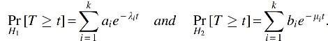
If N samples are observed from either H₁ or H₂, each with prior probability 1/2, then the Bayes error rate for any classifier that distinguishes H₁ from H₂ is at least $\frac{1 - δ}{2}$ , where

Table 1 shows examples of this lower bound for small values of k.

Table 1.
Sample Lower Bounds of Theorem 2.4

k Sample lower bound (from Theorem 2.4)

5 4.531 × 10⁷

7 9.665 × 10¹⁰

9 1.008 × 10¹⁴

k	Sample lower bound (from Theorem 2.4)
5	4.531 × 10⁷
7	9.665 × 10¹⁰
9	1.008 × 10¹⁴

We instantiate the bounds with α = 1/k, m = 2k, Δ = 1/(4k), and δ = 1/2, and solve for N in Equation (4) to get the required number of samples N₀.

Remark 3. From the square-root dependence of N in Theorem 2.3, the required number of samples N₀ has rate 4k in the exponent of $\frac{2 e}{Δ}$ if one just wants to learn the λ's, and Theorem 2.4 confirms that the exponent 4k is tight for learning the λ's.

Next, we state an additional information-theoretic lower bound showing that the information-theoretic (minimax) rate is necessarily of the form $\frac{1}{\sqrt{N}} Δ^{- O (k)}$ up to lower order terms, even if all of the λ_i are already known and we are only asked to reconstruct the mixing weights p_j.

Theorem 2.5. Let m, k be positive integers such that m > k > 3 and let Δ = 2/(m + k). There exists a fixed choice of λ₁, … , λ_k which are Δ-separated such that

where the max is taken over feasible choices of p, and the infimum is taken over possible estimators $\hat{p}$ from N samples of the mixture of exponentials with CDF $F (t) = 1 - \sum_{j} p_{j} e^{- λ_{j} t}$ .

Remark 4. Theorem 2.3 tells us that the number of samples needed (N) has exponent 4k when learning just the λ's and 6k for learning both the λ's and the p's. The exponent 2k in Theorem 2.5 suggests that the discrepancy of 2k for MPM in Theorem 2.3 is tight.

As expected, our lower bounds show that the learning problem becomes harder as Δ approaches 0. The “easiest” case, then, ought to be when Δ is as large as possible, so that the λ_i are equally spaced apart in the unit interval. This raises the following question: as Δ grows, does the sample complexity remain exponential in k, or is there a phase transition [as is the case in super-resolution, from Moitra (2015)] where the problem becomes easier? In the Supplementary Appendix, we completely resolve this question: the sample complexity still grows exponentially in 4k (Theorem D.7) even when Δ is maximally large.

2.4. A tight upper bound: Nazarov–Turán-based hypothesis testing

As an alternative to the learning problem that the Matrix Pencil Method solves, we also consider the hypothesis testing scenario in which we want to test if the sampled data match a hypothesized mixture distribution. In this case, we can give guarantees from weaker assumptions and requiring smaller numbers of samples. To state our guarantee, we need the following additional notation: for P a mixture of exponentials, let p_λ(P) denote the coefficient of e^−λt, which is 0 if this component is not present in the mixture. We study the following simple-versus-composite hypothesis testing problem using N samples:

Problem 1. Fix k₀, k₁, δ, Δ > 0 and let P be a known mixture of k₀ exponentials.

H₀: The sampled data are drawn from P.

H₁: The sampled data are drawn from a different unknown mixture of at most k₁ exponentials Q. Let $ν_{1} : = \max {λ : p_{λ} (P) > p_{λ} (Q)}$ and $ν_{2} : = \max {λ : p_{λ} (Q) > p_{λ} (P)}$ . We assume that $\min {| p_{ν_{1}} (P) - p_{ν_{1}} (Q) |, | p_{ν_{2}} (P) - p_{ν_{2}} (Q) |} \geq δ$ and |ν₁ − ν₂| ≥ Δ.

Henceforth, we will refer to H₀ as the null hypothesis and H₁ as the alternative hypothesis (note that H₁ is a composite hypothesis). To solve this hypothesis testing problem, we propose a finite-sample variant of the Kolmogorov–Smirnov test:

1.
Let α > 0 be the significance level.
2.
Let F_N be the empirical CDF and let F be the CDF under the null hypothesis H₀.
3.
Reject H₀ if ${sup}_{t} | F_{n} (t) - F (t) | > \sqrt{l og (2 ∕ α) ∕ 2 N}$ .

We show that this test comes with a provable finite-sample guarantee.

Theorem 2.6. Consider the problem setup as in Problem 1 and fix a significance level α > 0. Let $k : = \frac{k_{0} + k_{1}}{2}$ and $c_{Δ} = 8 e^{2} ∕ min (1 ∕ Δ, 2 k - 1)$ . Then:
1. (Type I Error) Under the null hypothesis, the above test rejects H ₀ with probability at most α.

2. (Type II Error) There exists $N_{0} (α) = O ({(c_{Δ} / Δ)}^{4 k - 2} \log (2 / α) / δ^{2})$ such that if N ≥ N ₀ , then the power of the test at significance level α is at least:

The full proof of Theorem 2.6 is given in Supplementary Appendix E. The key step in the proof is a careful application of the celebrated Nazarov–Turán lemma (Nazarov, 1993).

Remark 5. This improves upon the Matrix Pencil Method upper bound (Theorem 2.3), in terms of the exponent found above Δ (Δ^−6k vs. Δ^−4k) and above the mixing weights ( $p_{{min}^{4}}$ vs. δ²). Even when the alternative Q is fixed and known, we see from Theorem 2.4 that Ω((1/δ²)(1/Δ)^4k) many samples are information-theoretically required, which matches Theorem 2.6.
3. Simulations and Indistinguishability in Simple Examples

Our theoretical analysis rigorously establishes the worst-case dependence on the number of samples needed to learn the parameters of a single period of population history under our model—recall the construction of Theorem 2.4 of two hard-to-distinguish mixtures of exponentials and the result Theorem 2.2 converting these to population histories.

In our simulations, we will analyze both the performance and information-theoretic difficulty of learning not a specially constructed worst-case instance, but instead an extremely simple population history with k populations. More precisely we consider the following instance:

Simulation instance(k):

Population history description: We consider reconstructing a single period model with k populations in which the ratio of the population sizes is 1 : 2 : … :k and the relative probability of tracing back to each of these populations (i.e., $P r (ℰ_{i, i} | T > t_{0})$ from Supplementary Appendix A) are all equal to 1/k². This can easily be realized as a one period of a two-period population history model, in which in the second (more recent) era all populations are the same size.**

Mixture of exponentials description: We consider the following mixture of exponentials:

The constant term represents atomic mass at ∞ and corresponds to no coalescence. When k = 1 this is a standard exponential distribution; otherwise, it is a mixture of k + 1 exponentials, counting the degenerate constant term.

We do not believe that this is an unusually difficult instance of a mixture of exponentials on k components. If anything, the situation is likely the opposite: our worst-case analysis (Theorems 2.3 and 2.5) suggests that this is comparatively easy as the gap parameter Δ is maximally large.

To evaluate the error in parameter space from the result of the learning algorithm, we adopted a natural metric, the well-known Earthmover's distance. Informally, this measures the minimum distance (weighted by p_i and recovered ${\tilde{p}}_{i}$ ) that the recovered exponents must be moved to agree with the ground truth; we give the precise definition in Supplementary Appendix G.2.

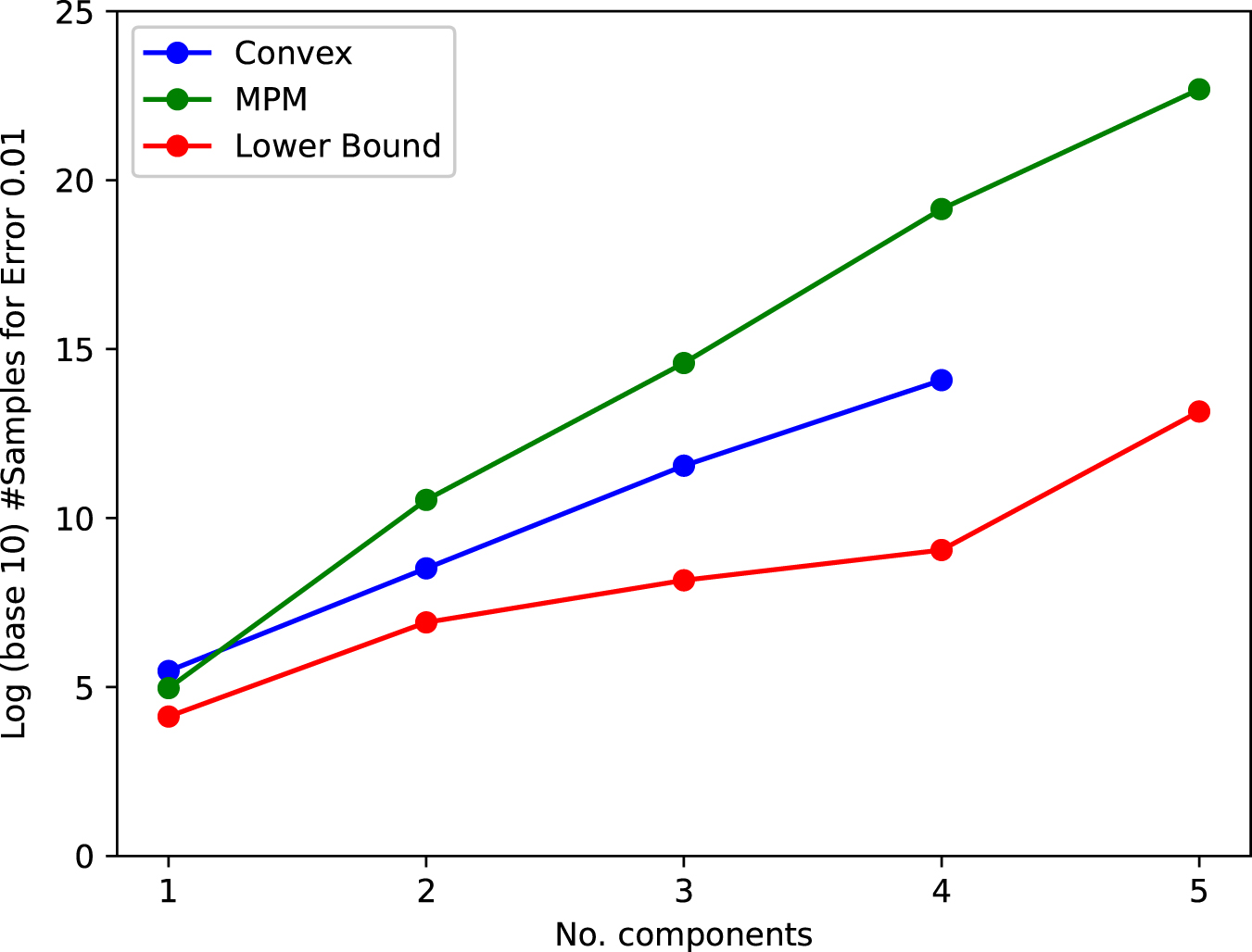
For a point of comparison with MPM, we also tested a natural convex programming formulation that essentially minimizes ${∥\int e^{- λ t} d μ (λ) - (1 - \tilde{F} (t))∥}_{\infty}$ over probability measures μ on $ℛ_{\geq 0}$ , where $\tilde{F}$ is the empirical CDF—refer to Supplementary Appendix G.1 for details. The results of running both the convex program and the MPM are shown in Figure 2 (blue and green lines) and in Table 2 on a log (base 10) scale; details of the setup are provided in Supplementary Appendix G.2. As expected, based on our theoretical analysis, the number of samples needed scaled exponentially in k, the number of populations in our instance. Owing to limitations of machine precision, the convex program could not reliably reconstruct at five components with any noise level and so this point is omitted.

FIG. 2.

Plot of #components versus log (base 10) number of samples needed for accurate reconstruction (parameters within Earthmover's distance 0.01). Below the red line, it is mathematically impossible for any method to distinguish with >75% success between the ground truth and a fixed alternative instance that has significantly different parameters.

Table 2.

Values (Before Log-Scale) in Figure 2

k	CVX	MPM	LB
1	2.98 × 10⁵	9.28 × 10⁴	1.34 × 10⁴
2	3.25 × 10⁸	3.45 × 10¹⁰	8.18 × 10⁶
3	3.55 × 10¹¹	3.87 × 10¹⁴	1.44 × 10⁸
4	1.21 × 10¹⁴	1.40 × 10¹⁹	1.13 × 10⁹
5	N/A	4.89 × 10²²	1.43 × 10¹³

CVX, convex program; LB, theoretical lower bound; MPM, Matrix Pencil Method.

Besides showing the performance of the algorithms, we were able to deduce rigorous unconditional lower bounds on the information-theoretic difficulty of these particular instances. Each point on the red line corresponds to the existence of a different mixture of exponentials (found by examining the output of the convex program), with a comparable number of mixture components,^†† which is far in parameter space^‡‡ from the ground truth and yet the distribution of N samples from this model (where N = 10^y and y is the y-coordinate in the plot) has total variation (TV) distance at most 0.5 from the distribution of N samples from the true distribution. By the Neyman–Pearson lemma, this implies that if the prior distribution is $(\frac{1}{2}, \frac{1}{2})$ between these two distributions, then we cannot successfully distinguish them with >75% probability. We describe the mathematical derivation of the TV bound in Supplementary Appendix G.2, and illustrate such a hard-to-distinguish pair in Example 1. Recall that by Theorem 2.2, such a hard-to-distinguish pair of mixtures can automatically be converted into a pair of hard-to-distinguish population histories.

Notably, the lower bound shows that reliably learning the underlying parameters in this simple model with five components necessarily requires at least 10 trillion samples from the true coalescence distribution. In reality, since we do not truly have access to clean i.i.d. samples from the distribution, this is likely a significant underestimate.

Example 1. Consider the mixtures of exponentials with CDFs F(t) and G(t), where 1 − F(t) = 0.5 + 0.25e^−0.5t + 0.25e^−t and

Despite being very different in parameter space, their H² distance is 7.9727 × 10⁻⁶ so any learning algorithm requires at least 15,660 samples to distinguish them with better than 75% success rate.

As a remark, we point out that the CDFs F and G in this example have exponents that are interlaced. Observe that this is a characteristic also shared by the information-theoretic obstructions referenced in Section 2.3 and Supplementary Appendix D. This likely illustrates a major source of difficulty of most reasonable-looking instances: “averaging” adjacent exponents of an exponential mixture typically produces a different mixture with a similar distribution whose components interlace with the original.

Footnotes

Author Disclosure Statement

The authors declare they have no conflicting financial interests.

Funding Information

Ankur Moitra was supported by a National Science Foundation CAREER Award CCF-1453261 and Large CCF-1565235, the David and Lucille Packard Fellowship, the Alfred P. Sloan Fellowship, and the Office of Naval Research Young Investigator award. Elchanan Mossel was supported by the Office of Naval Research N00014-16-1-2227, National Science Foundation CCF-1665252 and DMS-1737944 grants, and the Simons Investigator in Mathematics award 622132. Frederic Koehler was supported by Ankur Moitra's National Science Foundation Large CCF-1565235 grant and the David and Lucille Packard Fellowship. Govind Ramnarayan was supported by Elchanan Mossel's National Science Foundation CCF-1665252 and DMS-1737944 grants.

Supplementary Material

References

Bhaskar

, and Song

Y.S.

2014. Descartes' rule of signs and the identifiability of population demographic models from genomic variation data. Ann. Statist. 42, 2469.

Bhaskar

, Wang

Y.R.

, and Song

Y.S.

2015. Efficient inference of population size histories and locus-specific mutation rates from large-sample genomic variation data. Genome Res. 25, 268–279.

Blythe

R.A.

, and McKane

A.J.

2007. Stochastic models of evolution in genetics, ecology and linguistics. J. Stat. Mech. Theory Exp. 2007, P07018.

Candès

E.J.

, and Fernandez-Granda

2013. Super-resolution from noisy data. J. Fourier Anal. Appl. 19, 1229–1254.

Drummond

, Rambaut

, Shapiro

, et al. 2005. Bayesian coalescent inference of past population dynamics from molecular sequences. Mol. Biol. Evol. 22, 1185–1192.

Excoffier

, Dupanloup

, Huerta-Sánchez

, et al. 2013. Robust demographic inference from genomic and SNP data. PLoS Genet. 9, e1003905.

Feldmann

, and Whitt

1998. Fitting mixtures of exponentials to long-tail distributions to analyze network performance models. Perf. Eval. 31, 245–279.

Gautschi

1962. On inverses of vandermonde and confluent vandermonde matrices. Numer. Math. 4, 117–123.

Heled

, and Drummond

2008. Bayesian inference of population size history from multiple loci. BMC Evol. Biol. 8, 289.

10.

Hua

, and Sarkar

T.K.

1990. Matrix pencil method for estimating parameters of exponentially damped/undamped sinusoids in noise. IEEE Trans. Acous. Speech Signal Proc. 38, 814–824.

11.

Joseph

T.A.

, and Pe'er

2018. Inference of population structure from ancient DNA, 90–104. In RECOMB. Springer, Cham.

12.

Kim

, Mossel

, Rácz

M.Z.

, et al. 2015. Can one hear the shape of a population history? Theor. Popul. Biol. 100:26–38.

13.

, and Durbin

2011. Inference of human population history from individual whole-genome sequences. Nature, 475, 493.

14.

McVean

G.A.

, and Cardin

N.J.

2005. Approximating the coalescent with recombination. Philos. Trans. R. Soc. Lond. B Biol. Sci. 360, 1387–1393.

15.

Moitra

2015. Super-resolution, extremal functions and the condition number of vandermonde matrices, 821–830. Proceedings of the Forty-seventh Annual ACM Symposium on Theory of Computing, STOC 2015, ACM, New York, NY.

16.

Myers

, Fefferman

, and Patterson

2008. Can one learn history from the allelic spectrum?. Theor. Popul. Biol. 73, 342–348.

17.

Nazarov

F.L.

1993. Local estimates for exponential polynomials and their applications to inequalities of the uncertainty principle type. Algebra i Analiz, 5, 3–66.

18.

Nielsen

2000. Estimation of population parameters and recombination rates from single nucleotide polymorphisms. Genetics, 154, 931–942.

19.

Nordborg

2001. Coalescent theory. Handb. Stat. Genet. 2, 843–877.

20.

Prony

1795. Essai xperimental et analytique: sur les lois de la dilatabilit de uides lastique et sur celles de la force expansive de la vapeur de l'alkool, direntes tempratures. J. Ec. Polytech. Math. 1, 24–76.

21.

Schiffels

, and Durbin

2014. Inferring human population size and separation history from multiple genome sequences. Nat. Genet. 46, 919.

22.

Sheehan

, Harris

, and Song

Y.S.

2013. Estimating variable effective population sizes from multiple genomes: A sequentially Markov conditional sampling distribution approach. Genetics, 194, 647–662.

23.

Terhorst

, Kamm

J.A.

, and Song

Y.S.

2017. Robust and scalable inference of population history from hundreds of unphased whole genomes. Nat. Genet. 49, 303.

24.

Terhorst

, and Song

Y.S.

2015. Fundamental limits on the accuracy of demographic inference based on the sample frequency spectrum. Proc. Natl. Acad. Sci. U. S. A. 112, 7677–7682.

25.

Turán

1984. On a New Method of Analysis and Its Applications. Wiley New York, New York, NY.

Supplementary Material

Please find the following supplemental material available below.

For Open Access articles published under a Creative Commons License, all supplemental material carries the same license as the article it is associated with.

For non-Open Access articles published, all supplemental material carries a non-exclusive license, and permission requests for re-use of supplemental material or any part of supplemental material shall be sent directly to the copyright owner as specified in the copyright notice associated with the article.

0.00 MB

0.39 MB

How Many Subpopulations Is Too Many? Exponential Lower Bounds for Inferring Population Histories

Abstract

1. Introduction

1.1. Background: inference of population size history

1.2. Our setting: inference of multiple subpopulation histories

1.3. Modeling assumptions

1.3.1. The Multiple-Subpopulation Coalescent Model

1.4.1. Discussion of results

1.5. Related works

2. Theoretical Discussion

2.1. Reductions between mixtures of exponentials and population history

2.2. Guaranteed recovery of exponential mixtures through the Matrix Pencil Method

2.3. Strong information-theoretic lower bounds

Table 1. Sample Lower Bounds of Theorem 2.4 k Sample lower bound (from Theorem 2.4) 5 4.531 × 107 7 9.665 × 1010 9 1.008 × 1014

Footnotes

Author Disclosure Statement

Funding Information

Supplementary Material

References

Supplementary Material

Table 1.
Sample Lower Bounds of Theorem 2.4

k Sample lower bound (from Theorem 2.4)

5 4.531 × 10⁷

7 9.665 × 10¹⁰

9 1.008 × 10¹⁴