Evolutionary Switches Structural Transitions via Coarse-Grained Models

Abstract

Transitions between different conformational states are ubiquitous in proteins. A vast class of conformation-changing proteins includes evolutionary switches, which vary their conformation as an effect of few mutations or weak environmental variations. However, modeling those processes is extremely difficult due to the need of efficiently exploring a vast conformational space to look for the actual transition path. In this study, we report a strategy that simplifies this task attacking the complexity on several sides. We first apply a minimalist coarse-grained model to the protein, based on an empirical force field with a partial structural bias toward one or both the reference structures. We then explore the transition paths by means of stochastic molecular dynamics and select representative structures by means of a principal path-based clustering algorithm. We finally compare this trajectory with that produced by independent methods adopting a morphing-oriented approach. Our analysis indicates that the minimalist model returns trajectories capable of exploring intermediate states with physical meaning, retaining a very low computational cost, which can allow systematic and extensive exploration of the multistable proteins transition pathways.

1. Introduction

Signaling is a core activity in cells, usually regulated by bi- (or multi-) stable proteins, which can undergo conformational transitions in response to changes in environmental conditions or stimuli of different origin (Grant et al., 2010), including enzymes (Tozzini et al., 2007; Tamazian et al., 2015), transducers (Lia et al., 2014), and receptors (Weis and Kobilka, 2008). Most of these owe their function to a small portion of their structure—the conformational switch—undergoing a profound change between the two basic secondary folds, that is, a helix-to-strand transition or vice versa (α↔β), which subsequently triggers a global conformational change. The outmost importance of this mechanism is confirmed by the fact that natural evolution has extensively explored it, giving rise to the class of the evolutionary switches (Ugalde et al., 2004; Sikosek et al., 2016) in which the α versus β fold stability is driven by mutations.

In some cases, the genetic engineering has filled the gaps left by the natural evolution (Alexander et al., 2007, 2009). For instance, a continuous change from the 4β+α fold of the IgG binding domain of Streptococcus protein G (Gallagher et al., 1994) to the 3α fold of the human serum albumin binding domain (He et al., 2006) was realized by designed mutations in this ∼60 residue long polypeptide. It was subsequently demonstrated that the crossing point between the twofolds can be realized in this sequence by different mutations, creating couples of single residue mutants with bistable folds (He et al., 2012). This genetic engineering approach corresponds to a more or less systematic exploration of the multivariate space of amino acid sequence to build a sort of α/β transition phase diagram.

Clearly, the complete study of this phase diagram would greatly benefit of computer simulations (Tozzini, 2010). While a direct atomistic approach is limited both by the large extension of the space to explore—that is, the product of the conformational space with the sequence space—and by the difficulty to reproduce accurately the α/β stability in standard atomistic force fields (FFs) (Chen and Elber, 2014), a hybrid approach combining atomistic representation with Cα-based coarse-grained (CG) Go-models (Hills and Brooks, 2009) has recently been applied to the problem (Sikosek et al., 2016).

Similar to other partially biased models (Whitford et al., 2009; Trovato et al., 2013), in this work, a bias toward the correct α or β fold using a dual-basin formalism is superimposed to unbiased FF terms (Knott and Best, 2014), which include the sequence information. This approach, after a preliminary calibration of the relative energy of the two α and β attractive basins, leads to a reasonable correlation with experimental observation, although the full exploration of the sequence/structure space is still limited by the atomistic approach. Nevertheless, it seems winning in this approach the idea of separating structural and sequential information. This stems from the empirical observation that, in general, one can distinguish two determinants of the proteins structure: the first is the tendency of single amino acids or short sequences to be helix or strand formers, which has led to the elaboration and implementation of a number of secondary structure prediction algorithms (Cuff et al., 1998; McGuffin et al., 2000). The second is the global stabilization due to nonlocal contacts. The final fold, including secondary and tertiary structure, is determined by the interplay between these two factors, especially in the cases, often occurring in the switch proteins, where the helix/strand tendency is unclear.

In this work, we follow this reasoning line and adopt a conceptually similar strategy to that of Sikosek et al. (2016). But at variance with that, we consider a fully reductionist approach keeping only the essential elements and parameters. First, we consider the Cα-only-based representation of the polypeptide, also called “minimalist” coarse grained (MCG) (Trovato and Tozzini, 2012), which was demonstrated to be the simplest possible still capable of accounting uniquely of the secondary structure (Spampinato et al., 2014), and allowing the reconstruction of the atomistic backbone structure (Tozzini et al., 2006). This representation displays a great flexibility, being capable of easily passing from structurally biased [Go or network models (Tirion, 1996)] to unbiased (Yap et al., 2008) or partially biased parameterizations (Di Fenza et al., 2009). The latter (Trovato et al., 2013; Maccari et al., 2014) typically retain a bias in the local part of the nonbonded contacts maps to accurately account for the hydrogen bond network (Tozzini and McCammon, 2005). The level of bias can be tuned in the different terms of the FF, as far as the functional forms, including multistability through the bias toward two or more reference structures (Tavanti and Tozzini, 2014).

Using the minimalist representation, here, we report a strategy to build models for the evolutionary switches gradually decreasing the level of bias and including the sequence information. We first present and analyze the behavior of the basic model, consisting of two separated submodels with bias toward the two extreme switch structures; we then combine the two submodels in a bistable one, including two-basins potentials in the local terms, and illustrate how to include the sequence dependence in the bonded terms. Given the extreme simplicity, this model allows a fast exploration of the configuration/sequence space, which we perform combining molecular dynamics simulations with morphing-related methods (Krebs and Gerstein, 2000; Ye and Godzik, 2004), based on the optimal mass transport approach (Koshevoy et al., 2014; Tamazian et al., 2015), including physical constraints of geometric nature (Evans and Gangbo, 1999), and with the minimal action path search (Franklin et al., 2007). The next section describes the Methods, the subsequent the Results, Conclusions, and perspectives follow.

2. Methods

2.1. Systems representations and FFs

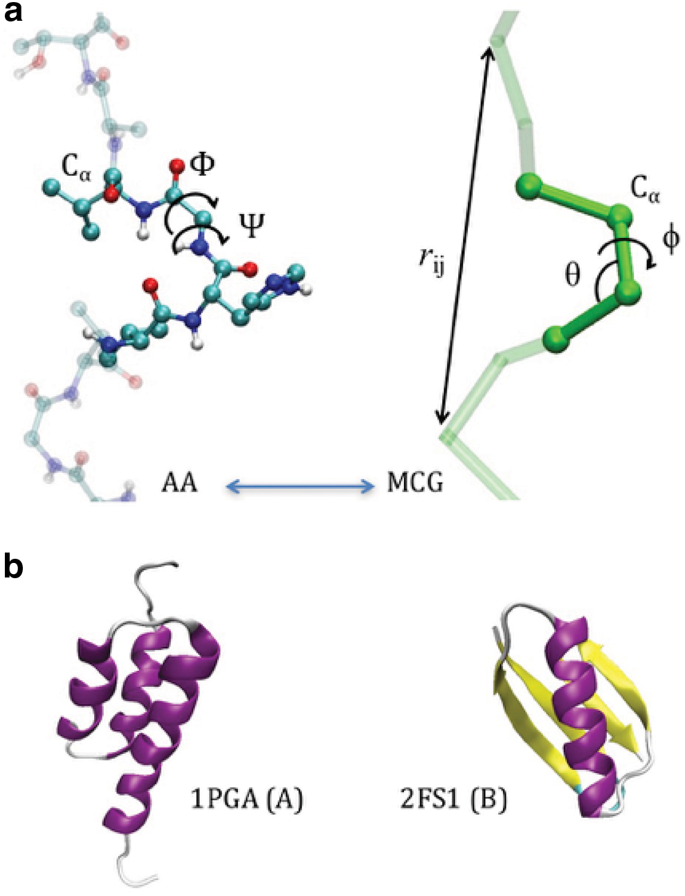
The MCG model is illustrated in Figure 1a: the passage from the atomistic representation to the minimalist CG one is obtained retaining only the Cα as interacting centers (“beads”), in which the whole amino acid mass is concentrated. The internal coordinates are the Cα-Cα distances, d, the three-Cαs pseudo-bond angles, θ, and the four-Cαs pseudo dihedral, φ. The reduction of degrees of freedom from the AA to the MCG representation is of about three orders of magnitude, considering also the solvent implicit treatment. In the atomistic representations, the backbone conformation is determined by the sequence of Ramachandran dihedrals (Φ_i, Ψ_i) describing the rotation of peptide planes hinging on the ith Cα. This makes the Ramachandran map (RM)—the scatter plot of (Φ, Ψ)—a useful representation of the secondary structure. In the minimalist model, the Cα-Cα distance is basically fixed by the rigidity of the peptide bond (and treated with an holonomic constrain), and the backbone conformation is described by the (θ_i, φ_i) angles sequence. It was shown (Tozzini et al., 2006) that the (θ, φ) scatter plot can take the role of the RM for MCG models. The interaction terms are separated in “bonded” and “nonbonded”

FIG. 1.

(a) Atomistic (left) and MCG (right) representation of the polypeptide chain. The internal coordinates are reported. (b) Reference structures used for the evolutionary switch model. Left, wild type (WT) of human serum albumin binding protein (He et al., 2006), the A reference model, and IgG binding domain of Streptococcus protein G (Gallagher et al., 1994), the B reference model. Protein data bank codes are reported.* MCG, “minimalist” coarse grained.

\begin{matrix} U = \underset{̲}{\sum_{b o n d a n g l e s} u_{i}^{θ} (θ_{i}) + \sum_{d i h e d r a l s} u_{i}^{ϕ} (ϕ_{i})} + \sum_{i > j} u^{n b} (r_{i j}) \\ b o n d e d i n t e r a c t i o n s \end{matrix}

(1)

the “bonded” terms representing the chemical interaction, or topology of the connections, are described via the local internal coordinates. The “nonbonded” (u^nb) term includes, besides steric hindrance and (screened) electrostatics, hydrophobic interactions and hydrogen bonds, whose geometry is very complex, yet critical to accurately account for the protein structure. This term is conveniently split in local and nonlocal contributions $\sum u^{n b} (r_{i j}) = \sum_{(i, j) \in L} u_{l o c a l} (r_{i j}) + \sum_{(i, j) \notin L} u_{n l} (r_{i j})$ (2)

L being a set of “local nonbonded contacts,” typically including the hydrogen bond network, disulfide, and salt bridges or other persistent and strong contacts. u_local is the term usually retaining the bias toward the reference structure (Tozzini et al., 2007; Trovato et al., 2013; Spampinato et al., 2014), bringing structural accuracy to the model. The set of local contacts can be defined either geometrically based on a cutoff distance (Di Fenza et al., 2009) or on chemical–physical considerations (Trovato et al., 2013), for example, the known network of H-bonds (Tozzini et al., 2006) and different functional forms were previously used, either generic single well potentials (Di Fenza et al., 2009) or more sophisticated amino acid-dependent potentials including sequence information, electrostatics, hydrophobicity, and desolvation effects (Trovato et al., 2013). This term should be considered the equivalent of the biased multi-basin one in Sikosek et al. (2016). Conversely, u_nl is a standard nonbonded two body term defined based on the bead-couple type.

In this work, we start from the simplest basic model and gradually include the complexity. We use as the reference case the well-studied Ig/Albumin switch of Gallagher et al. (1994) and He et al. (2006) (structures in Fig. 1b). We first create two reference models partially biased toward the two reference structures A and B of Figure 1b. We use the parameterization previously tested on other proteins (Di Fenza et al., 2009). Briefly, u_θ and u_φ are represented by anharmonic terms accurately describing the secondary structures; the u_nb terms both local and nonlocal are represented by a Morse potential, but while the nonlocal part is a generic non-biased, the local contacts—defined through a geometric criterion¹—have equilibrium distance set at the reference structure. The force constants are previously optimized and are reported together with other details in previous works (Delfino et al., 2019) and in the Supplementary Material.

The two FFs named FF_A and FF_B are biased toward the two extreme folds, namely the 3α and the 4β+α, respectively. Here, we first explore the structural transitions, energy profiles, and so forth, produced by these two FFs. This can be considered the 0th step of a strategy to gradually decrease the bias consisting of the following steps: (1) include bistability and (2) release the structure dependence in favor of the sequence dependence in (a) the local terms and (b) the average-long range terms. In this work, we preliminarily explore step 1, while step 2 is currently in progress and will be the matter of a forthcoming article. The bistable field FF_AB is obtained by merging FF_A and FF_B according to the following algorithm: (1) the “bonded” terms u_θ and u_φ are replaced by double well-functional forms with basins corresponding to the single basin of the parent FFs; (2) the u_local terms are treated on a bead couple basis: for each given couple i, j, if it is present either in FF_A or in FF_B, it is added, if it is present in both, it is replaced by a double well potential with minima corresponding to those of the parent FFs; (3) the u_nl terms are left unchanged. A full description of the algorithm used to merge the two fields in the bistable one is reported in the Supplementary Material.

2.2. Simulations setup and data analysis

The conformational space is explored using different methods. Langevin molecular dynamics (LD)² is used to sample the transition paths at different temperatures (typically room temperature [RT] and low temperature [LT], 10K), starting from different conformations. As an alternative to the counting of native contacts (Sikosek et al., 2016), here, we define a parameter σ by means of a combination of the root mean squared deviation from A and B (RMSD_A,B) to measure the progression of the transition ${R M S D}_{A ∕ B} (r) = \sqrt{\frac{1}{N} \sum_{i} {(x_{i} - x_{i}^{A ∕ B})}^{2}} σ (r) = \frac{1}{2} (\frac{{R M S D}_{A} (r) - {R M S D}_{B} (r)}{{R M S D}_{A, B}}) + \frac{1}{2}$ (3)

σ assumes the value 0 in A and 1 in B and is evaluated along the trajectory. LD produces high statistics trajectories. To identify a limited number of relevant conformations, we applied the principal path (PP) clustering algorithm (Ferrarotti et al., 2019). Relevant quantities (e.g., energies and RMSD, σ values) are evaluated by means of cluster averages. Alternative averaging algorithms are used and compared with the clustering, based on the running averages of σ and of the energies (Delfino et al., 2019).

Transition paths are also searched for using algorithms exclusively based on the A and B structures. These are PROMPT (PRotein cOnformational Motion PredicTion³) (Tamazian et al., 2015) based on the minimization of a mass transport functional subject to restrains on the bond angles and dihedrals along the chain, and MAP (Minimal Action Path) (Franklin et al., 2007) based on the numerical solution of Euler equations of a simplified Lagrangian including harmonic networks to bias toward A and B states. Both methods are very computationally cheap and parameter free, and return an already cleaned up transition path, with no need of postprocessing (Delfino et al., 2019).

3. Results

3.1. Molecular dynamics

Figure 2 reports the LD results at different temperatures and with different FFs (simulation parameters reported in the caption). The simulation with FF_B (in green) is started from configuration A and vice versa (in red), so that the bias toward the opposite configuration induces the structural transition. The comparison of opposite transitions with same temperatures clearly shows that the A → B occurs more slowly and with a larger gain in energy with respect to the B→A. A deeper inspection of the energy terms (reported in the Supplementary Material) shows that the prevalent one is u_local, indicating that the hydrogen bond network of the β sheets in the B structure requires the formation of a larger number of contacts and less local along the chain and therefore slower to form than in the all-helical A structure. In both cases, the transition proceeds by a fast passage through an unfolded state (except for the central α-helix present in both structure, which remain folded) and refolding of the secondary structures, occurring in the first few hundreds fs (see structures reported in Fig. 1). Then, in the A → B case, the system passes from two distinct steps, that is, the formation of the two terminal hairpins, which finally joint to the four-strand sheet in the final structure. These steps are visible as plateau in the energy and σ plots especially in the LT simulation.

FIG. 2.

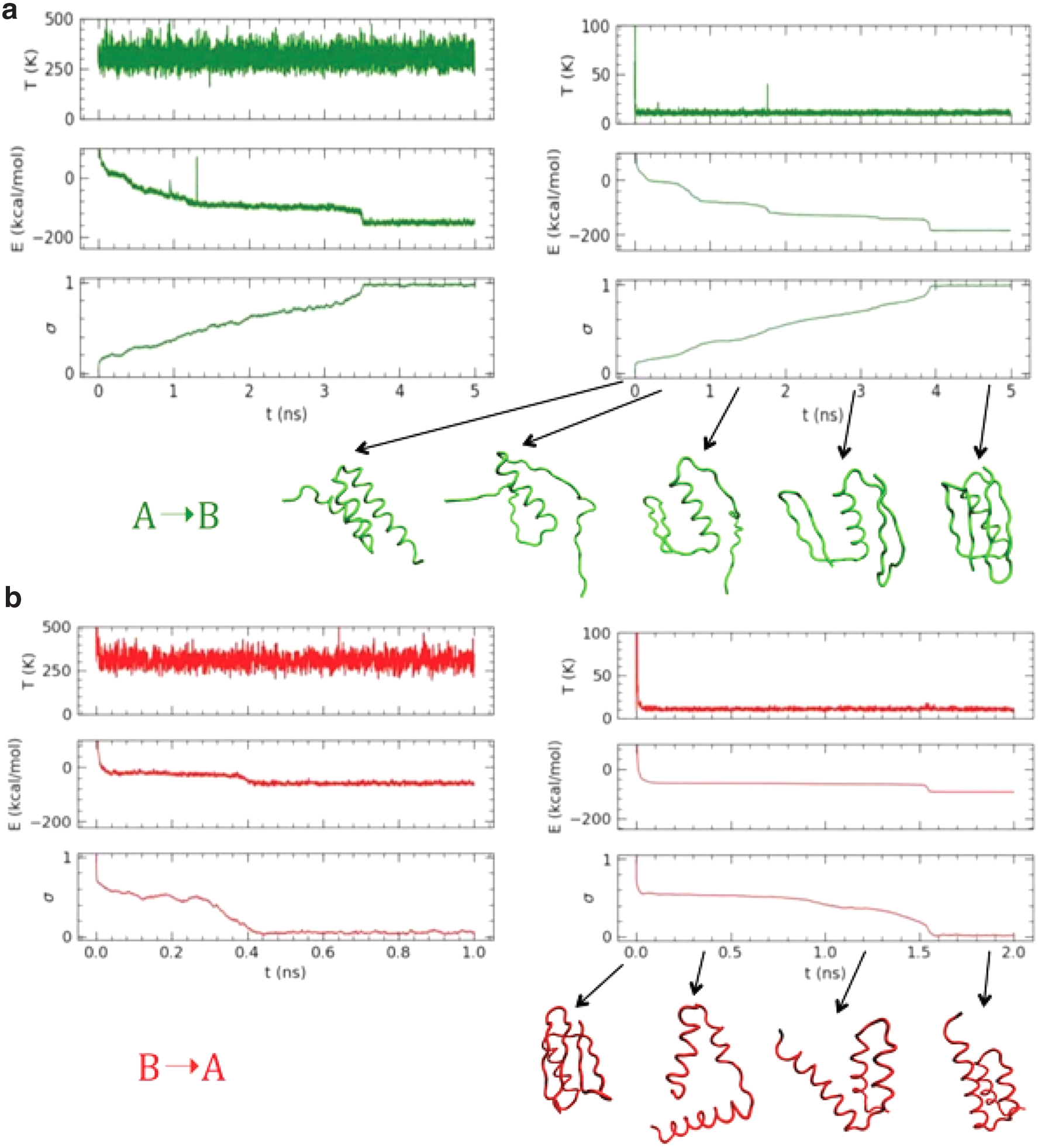
LD simulations with different FFs. (a) Simulations with FF_B, starting from A, at RT and at LT (10K) both with γ = 16 ps⁻¹. From top to bottom, temperature, total configuration energy, and σ are reported. Selected structures are reported with arrows indicating the approximate time frame. (b) Same for the FF_A starting from B, using γ = 2 ps⁻¹ for both RT and LT. FFs, force fields; LD, Langevin molecular dynamics; LT, low temperature; RT, room temperature.

In the B → A case, the intermediate steps are fewer and correspond to the subsequent compaction of the helices in the bundle, stabilized by interhelical contacts. These, however, are less strong and specific than the intersheet contacts in the β fold; therefore, the steps are less distinct. We remark at this point that these simulations should be regarded as folding steps of states A and B of the corresponding wild-type proteins (i.e., albumin binding-Ig binding domain G proteins) rather than A↔B structural transition occurring in bistable proteins. In fact, in these simulations, the local tendency to form helices or strands is strong and it is the first one manifesting during refolding, while the inter-secondary contacts form later.

3.2. Transition paths in the monostable fields

Figure 3 reports a representation of the transition path in the RMSD_A/B plane. The A structure is located in the upper-left part of the plane, and the B structure in the lower right. Figure 3a reports the scatter plot of the 10K simulation and the dots corresponding to PP clusters evaluated along it. The steps revealed by the plateau in the LD simulations are visible and persist even in the RT simulation (Fig. 3b), although the larger fluctuations allow a more extensive exploration of conformations. In both the RT and LT simulations, the structures are free of steric clashes and, upon backbone rebuilding, the RM reveal no relevant presence of forbidden conformations (RM reported in the Supplementary Material). The fact that FF_A and FF_B simulations follow two different paths is confirmed because red and green lines occupy different regions of the plot, and the conformations are different even in their crossing point, although they both represent a rather unfolded and expanded structure.

FIG. 3.

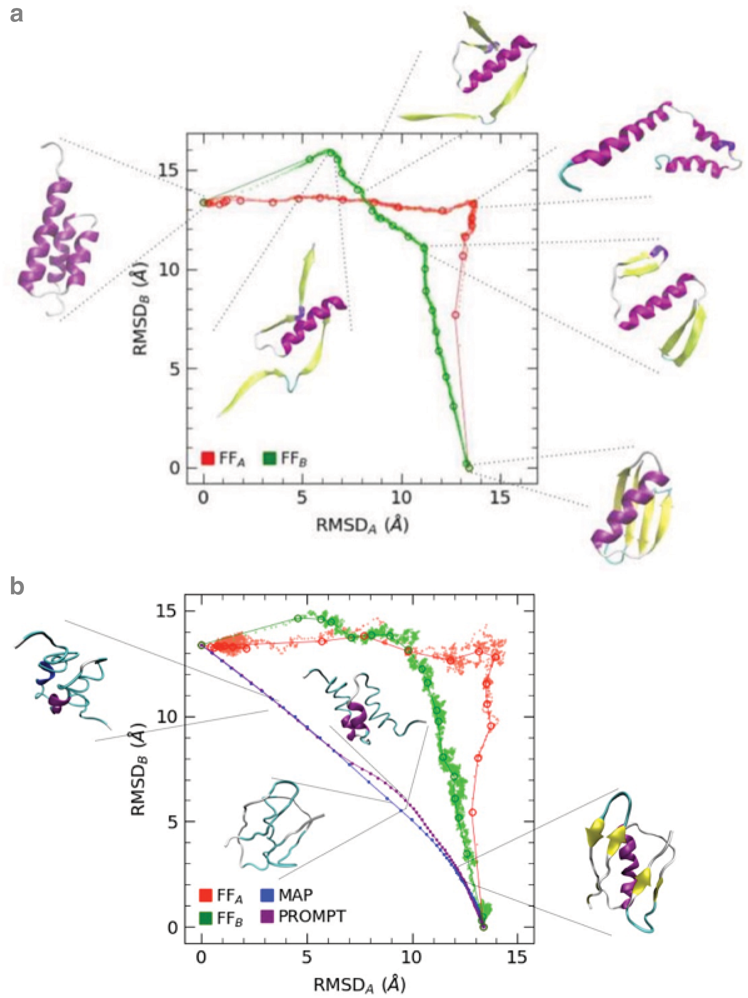
Transition paths evaluated with FF_A, FF_B, MAP, and PROMPT. (a) LD simulations at 10K and (b) LD simulation at RT superimposed to MAP and PROMPT. Selected structures are reported indicating the point to which they correspond.

Figure 3b also reports the comparison with MAP and PROMPT trajectories. These appear to occupy regions much nearer to the diagonal and therefore both nearer to both A and B. Their appearance is more similar to random coils, which is what one would expect as a transition state during an A-B switching process. However, an inspection to these structures reveals that they are less physical.

3.3. The bistable field: preliminary steps

Figure 4 reports the representation of the transition paths produced by RT simulations (starting from A, green, and from B, red) using the merged field obtained as explained in Section 2. No additional parameter is added; therefore, the relative stability of the two structures is determined by the relative weight of the bonded and local terms in the parent fields. An analysis of the energy terms along the two simulations starting from A and from B (reported in the Supplementary Material) shows that angle/dihedral terms and the local nonbonded interactions act in the opposite way to this respect: the angle/dihedral terms tend to stabilize the helical A form, whereas the Morse local contacts are more and more stable in the B form. If no parameters are added, the latter wins, making the B form more stable of about 50 kcal/mol. This relative stability of the two structures can be tuned manipulating the relative weight especially of the local Morse terms and is part of the step 2 of the FF optimization, since it must be carried out in a sequence-dependent way. These aspects, as long as all the others related to the optimization of the bistable field in a sequence-dependent way, are beyond the scope of this preliminary work and will be addressed in a forthcoming article.

FIG. 4.

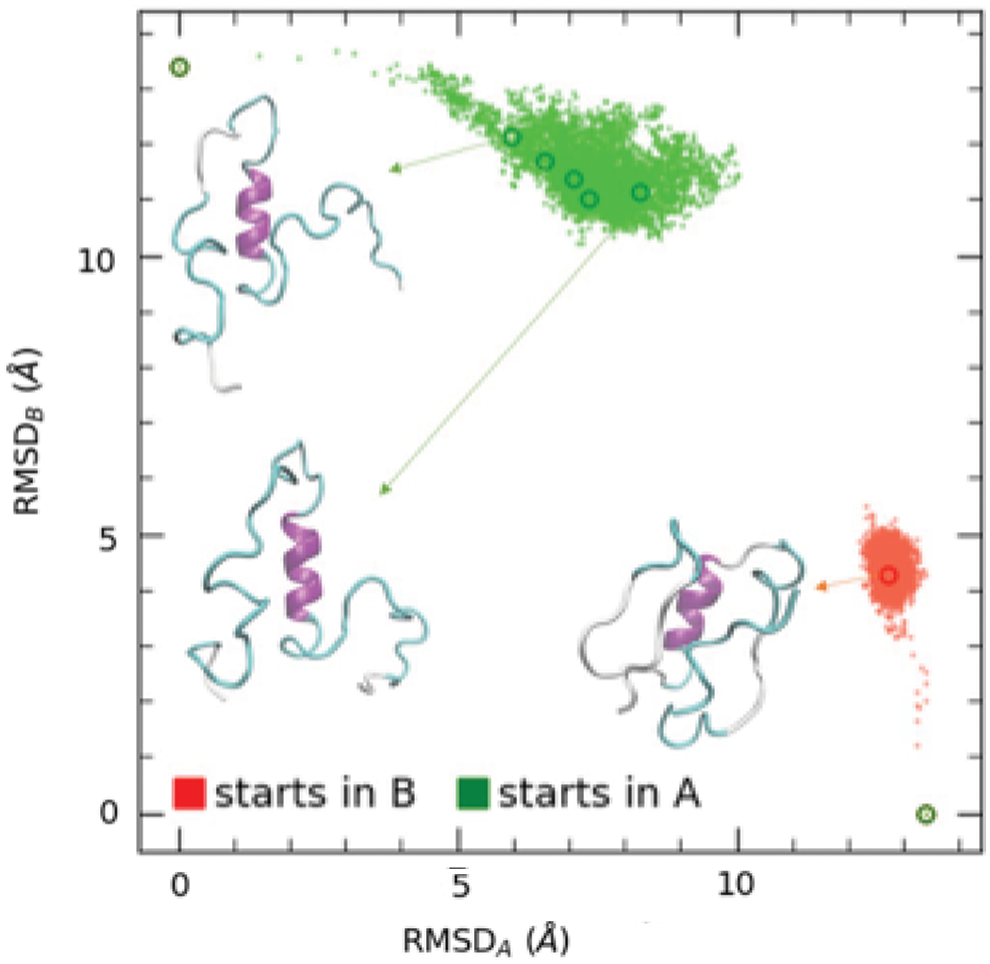
Transition paths evaluated with the bistable FF. Red: starting from B structure, green: starting from A structure. Representative structures of the intermediates are reported.

The analysis of the transition paths of Figure 4 reveals again that physically sound conformations are explored during simulations. At variance with the simulations with monostable fields, in this case, the complete transition is not reached as an effect of the total bias elimination; however, two distinct and well-defined structural clusters are explored starting from conformation A (green) and B (red), respectively. The cluster explored from the simulation starting from A is roughly located in the same RMSD_AB plane region of simulations with the monostable FF_B field (green in Fig. 3), and the corresponding representative structures are similar, although in those from the bistable FF, the two unfolded sheets appear more random coil-like than those of the monostable FF_B. Conversely, the cluster explored in the simulation with the bistable FF starting from B is located in a different region of the plot and appears quite different from that of the monostable FF_A (red in Fig. 3), being more compact and preserving some sheet-like structure, although distorted. Overall, the effect of the introduced bistability appears to be a general “randomization” of the intermediate structures toward random coil-like intermediates, whereas in the monostable FFs simulations, the secondary features seems more persistent.

4. Summary and Perspectives

We have reported a simulation study of the 3α↔4β+α structural transition in an exemplar evolutionary switch performed with a minimalist CG Cα-based model. Stochastic dynamics RT simulations are reported and compared with results of direct path search methods (MAP and PROMPT). Results from the totally biased CG FF toward A and B structures are able to fully sample the transition paths (if started from the opposite structure than the reference one), exploring different intermediates en passant, which, however, preserve the secondary features of the parent FF. Conversely, the intermediates from bistable FF appear more random coil-like. In both cases, however, the dynamical simulations are shown to efficiently explore a vast region of the conformational space, farther from the A-to-B diagonal than the PROMPT and MAP methods, resulting in structurally reasonable conformations, as validated by reconstructed RMs. The use of direct path search methods gives interesting results, being automatically free of the bias toward one or the other structures. However, a postprocessing is needed to eliminate steric clashes and too high structural distortions.

In the present form, the bistable FF stabilizes the β-prevalent B form. However, the extreme simplicity of the model gives a large flexibility to the parameterization, which allows highly tunable different balance between the topological (i.e., chemical connected or bonded interactions), and nonbonded local or nonlocal terms. This information can be included in the model in a sequence dependent way to reproduce the different α/β propensities in the evolutionary switch family in the following ways: (1) the helical/strand propensity can be included in the bond angles/dihedral and u^loc term, using secondary propensity known probabilities; (2) the amino acid-type potentials can be used in u^nb, which automatically include the sequence dependent in average-long range contacts. An extensive study exploring the interplay between topological and average-long range interactions in the determination of the final fold is currently in the course and is the matter of a forthcoming article (Delfino et al., n.d.).

Footnotes

Acknowledgment

We thank Dr. Giuseppe Maccari for useful discussions and for support with SecStAnT code.

Authors' Contributions

The article was written through contributions of all authors. F.D. and Y.P. have given equal contribution. All authors have given approval to the final version of the article.

Author Disclosure Statement

The authors declare they have no competing financial interests.

Funding Information

The work of E.S. has been supported by the RSF grant 19-71-30020 “Applications of probabilistic artificial neural generative models to development of digital twin technology for non linear stochastic systems” (HSE University).

Supplementary Material

References

Alexander

P.A.

, He

, Chen

, et al. 2007. The design and characterization of two proteins with 88% sequence identity but different structure and function. Proc. Natl. Acad. Sci. U S A. 104, 11963–11968.

Alexander

P.A.

, He

, Chen

, et al. 2009. A minimal sequence code for switching protein structure and function. Proc. Natl. Acad. Sci. U S A. 106, 21149–21154.

Boateng

, and Todorov

2015. Arbitrary order permanent Cartesian multipolar electrostatic interactions. J. Chem. Phys. 142, 034117.

Bush

, Todorov

, and Smith

2006. A DAFT DL_POLY1 distributed memory adaptation of the smoothed particle mesh Ewald method. Comp. Phys. Commun. 175, 323–329.

Chen

, and Elber

2014. The energy landscape of a protein switch. Phys. Chem. Chem. Phys. 16, 6407–6421.

Cuff

J.A.

, Clamp

M.E.

, Siddiqui

A.S.

, et al. 1998. JPred: A consensus secondary structure prediction server. Bioinformatics, 14, 892–893.

Delfino

, Porozov

, Stepanov

, et al. 2019. Structural transition states explored with minimalist coarse grained models: Applications to Calmodulin. Front. Mol. Biosci. 6, 104.

Delfino

, et al. n.d. Exploring the phase diagram of evolutionary switches with a minimalist model. In preparation.

Di Fenza

, Rocchia

, and Tozzini

2009. Complexes of HIV-1 integrase with HAT proteins: Multiscale models, dynamics, and hypotheses on allosteric sites of inhibition. Proteins, 76, 946–958.

10.

Evans

L.C.

, and Gangbo

1999. Differential equations methods for the Monge-Kantorovich mass transfer problem. Am. Math. Soc. 137, 1–66.

11.

Ferrarotti

, Rocchia

, and Decherchi

2019. Finding principal paths in data space. IEEE Trans. Neural Netw. Learn. Syst. 30, 2449–2462.

12.

Franklin

, Koehl

, Doniach

, et al. 2007. MinActionPath: Maximum likelihood trajectory for large-scale structural transitions in a coarse-grained locally harmonic energy landscape. Nucleic Acid Res. 35, W477–W482.

13.

Gallagher

, Alexander

, Bryan

, et al. 1994. Two crystal structures of the B1 immunoglobulin-binding domain of streptococcal protein G and comparison with NMR. Biochemistry, 33, 4721–4729.

14.

Grant

, Gorfe

, and McCammon

2010. Large conformational changes in proteins: Signaling and other functions. PLoS Comput. Biol. 20, 142–147.

15.

, Chen

, Alexander

P.A.

, et al. 2012. Mutational tipping points for switching protein folds and functions. Structure, 20, 283–291.

16.

, Rozak

D.A.

, Sari

, et al. 2006. Structure, dynamics, and stability variation in bacterial albumin binding modules: Implications for species specificity. Biochemistry, 45, 10102–10109.

17.

Hills

, and Brooks

2009. Insights from coarse-grained Gō models for protein folding and dynamics. Int. J. Mol. Sci. 10, 889–905.

18.

Knott

, and Best

2014. Discriminating binding mechanisms of an intrinsically disordered protein via a multistate coarse-grained model. J. Chem. Phys. 140, 175102.

19.

Koshevoy

A.A.

, Stepanov

E.O.

, and Porozov

Y.B.

2014. Method of prediction and optimization of conformational motion of proteins based on mass transportation principle. Biophysics, 59, 28–34.

20.

Krebs

, and Gerstein

2000. The morph server: A standardized system for analyzing and visualizing macromolecular motions in a database framework. Nucleic Acids Res. 28, 1665–1675.

21.

Lia

, Wanga

, and Takadab

2014. Energy landscape views for interplays among folding, binding, and allostery of calmodulin domains. PNAS, 111, 10550–10555.

22.

Maccari

, Spampinato

, and Tozzini

2014. SecStAnT: Secondary Structure Analysis Tool for data selection, statistics and models building. Bioinformatics, 30, 668–674.

23.

McGuffin

, Bryson

, and Jones

2000. The PSIPRED protein structure prediction server. Bioinformatics, 16, 404–405.

24.

Sikosek

, Krobath

, and Chan

2016. Theoretical insights into the biophysics of protein bistability and evolutionary switches. PLoS Comput. Biol. 12, e1004960.

25.

Spampinato

, Maccari

, and Tozzini

2014. Minimalist model for the dynamics of helical polypeptides: A statistic-based parameterization. J. Chem. Theory Comput. 10, 3885–3895.

26.

Tamazian

, Ho Chang

, Knyazev

, et al. 2015. Modeling conformational redox-switch modulation of human succinic semialdehyde dehydrogenase. Proteins, 83, 2217–2229.

27.

Tavanti

, and Tozzini

2014. A multi-scale–multi-stable model for the rhodopsin photocycle. Molecules, 19, 14961–14978.

28.

Tirion

M.M.

1996. Large amplitude elastic motions in proteins from a single parameter, atomic analyses. Phys. Rev. Lett. 77, 1905–1908.

29.

Todorov

, Smith

. Trachenko

, et al. 2006. DL_POLY_3: New dimensions in molecular dynamics simulations via massive parallelism. J. Mater. Chem. 16, 1911–1918.

30.

Tozzini

2010. Minimalist models for proteins: A comparative analysis. Q. Rev. Biophys. 43, 333–371.

31.

Tozzini

, and McCammon

2005. A coarse grained model for the dynamics of flap opening in HIV-1 protease. Chem. Phys. Lett. 413, 123–128.

32.

Tozzini

, Rocchia

, and McCammon

2006. Mapping all-atom models onto one-bead coarse-grained models: General properties and applications to a minimal polypeptide model. J. Chem. Theory Comput. 2, 667–673.

33.

Tozzini

, Trylska

, Chang

, et al. 2007. Flap opening dynamics in HIV-1 protease explored with a coarse-grained model. J. Struct. Biol. 157, 606–615.

34.

Trovato

, Nifosì

, Di Fenza

, et al. 2013. A minimalist model of protein diffusion and interactions: The green fluorescent protein within the cytoplasm. Macromolecules, 46, 8311–8322.

35.

Trovato

, and Tozzini

2012. Minimalist models for biopolymers: Open problems, latest advances and perspectives. AIP Conf. Proc. 1456, 187–200.

36.

Ugalde

, Chang

, and Matz

2004. Evolution of coral pigments recreated. Science, 305, 1433.

37.

Weis

, and Kobilka

2008. Structural insights into G-protein-coupled receptor activation. Curr. Opin. Struct. Biol. 18, 734–740.

38.

Whitford

P.C.

, Noel

J.K.

, Gosavi

, et al. 2009. An all-atom structure based potential for proteins: Bridging minimal models with all-atom empirical forcefields. Proteins, 75, 430–441.

39.

Yap

, Lux Fawzi

, and Head-Gordon

, 2008. A coarse-grained α-carbon protein model with anisotropic hydrogen-bonding. Proteins, 70, 626–638.

40.

, and Godzik

2004. FATCAT: A web server for flexible structure comparison and structure similarity searching. Nucleic Acids Res. 32, W582–W585.

Supplementary Material

Please find the following supplemental material available below.

For Open Access articles published under a Creative Commons License, all supplemental material carries the same license as the article it is associated with.

For non-Open Access articles published, all supplemental material carries a non-exclusive license, and permission requests for re-use of supplemental material or any part of supplemental material shall be sent directly to the copyright owner as specified in the copyright notice associated with the article.

0.00 MB

0.47 MB