Conditional Random Fields with Least Absolute Shrinkage and Selection Operator to Classifying the Barley Genes Based on Expression Level Affected by the Fungal Infection

Abstract

The classical methods for the classification problem include hypothesis test with the Benjamini–Hochberg method, hidden Markov chain model, and support vector machine. One major application of the classification problem is gene expression analysis, for example, detecting the host genes having interaction with pathogen. The classical methods can be applied and have a good performance when the number of genes having interaction with the pathogen is not sparse with respect to the candidate genes. However, conditional random field (CRF), with an appropriate design, can be applied and have good performance even when it is sparse. In this work, we proposed a modified CRF with a baseline to reduce the number of parameters in CRF. Moreover, we show an application of CRF with the least absolute shrinkage and selection operator (LASSO) to classifying barley genes of its reaction to the pathogen.

1. Introduction

The conditional random field (CRF) was introduced by Sutton and McCallum (2012). The major reason why CRF is flexible is that we can define the feature functions base on the complexity of the problems with respect to the data set. With an appropriate design, CRF can fit into several different scenarios such as text process (Ammar et al., 2014), bioinformatics (Thiagarajan and Bremananth, 2015), and image process (Lu et al., 2018). However, because of the flexibility, the CRF usually contains a large number of parameters. This causes computational difficulty during the training step. CRF contains its own penalty to prevent overfitting; the penalty proposed in Sutton and McCallum (2012) considers the Euclidean distance (l₂-norm) of parameters. To enforce the sparsity of covariates in CRF, a stronger penalty (l₁-norm) of the parameters in CRF, least absolute shrinkage and selection operator (LASSO) penalty is applied (Hayashida et al., 2013).

This study demonstrates the flexibility of CRF and propose an improved CRF model with a fewer number of parameters by setting a baseline. An improved CRF model with LASSO is proposed for the barley gene expression data, which are collected to classify different reactions of host genes to pathogens to improve the immunity of barley. Since the gene expression levels on different time points for one host gene may have strong interdependence on each other, the classical classification method may not have a well-fit. We demonstrate an application of CRF with proper model specification and LASSO penalty to the barley data.

This work is organized as follows. Section 2 provides the experiment details of gene data. Section 3 shows the technical details about how to design CRF for this barley data and how to improve CRF and implement the LASSO into CRF. Section 4 demonstrates the performance of CRF by comparing it with support vector machine (SVM; Meyer et al., 2019) and generalized linear model (GLM) with LASSO (Friedman et al., 2010). Finally, we apply the CRF to the barley data and draw the conclusion in Section 5.

2. The Barley–Pathogen Interaction Experiment

An experiment was conducted by Dr. Shaobin Zhong's group in the Department of Plant Pathology at North Dakota State University to determine what genes in the barley genome will be changed at expression level during infection by the fungus Bipolaris sorokiniana causing the spot blotch disease. The study aimed to identify barley genes involved in host resistance or susceptibility to the disease. The information will allow us to have a better understanding of the interaction between the pathogen and the host and may help us to design new approaches for better control of the disease.

In this study, there are two treatments: Barley cv. Bowman infected by the original isolate (ND90Pr), which is highly virulent on Bowman, and the barley infected by the mutated isolate with low virulence on Bowman. The mutant was generated by deleting an NPS gene conforming high virulence of the isolate. For each treatment, three leaf samples were collected at 0, 6, 12, 18, 24, 36, 48, and 72 hours after inoculation. Hence, a total of 48 samples, that is, 3 replicates in 2 treatments at 8 time points are used to generate the data set.

In this experiment, the expression level of 6325 genes of Barley cv. Bowman are studied (Trapnell et al., 2012), and each contains 8 records collected at the 8 time points, respectively. When the gene expression level is missing in some of the 8 hours records, it is assumed to have a very low expression level and numerically set to 0. To analyze the data, the ratio between two treatments gene expression levels, namely, relative gene expression level, is used. The relative gene expression level is $g_{j} = \frac{{g'}_{j} + 10^{- 6}}{{g'}_{0} + 10^{- 6}},$

where $j = 0, 6, 12, 18, 24, 36, 48, 72$ , g_j is the relative gene expression level on the time j, and $g'_{j}$ is the raw gene expression level on the time j. To avoid the denominator of g_j equaling 0, $1 0^{- 6}$ is added.

After computing the relative gene expression level, the next problem is the large range of the data (from $4.5 \times 1 0^{- 11}$ to $1.4 \times 1 0^{10}$ ). This large range of data will cause the overflow problem. To overcome the overflow, we rescale the relative gene expression level to $8.2 \times 1 0^{- 17}$ $25, 000$ by multiplying $\frac{25, 000}{(1.4 \times 10^{10} - 4.5 \times 10^{- 11})}$ to the relative gene expression level (g_j).

After finishing all the data process, the next step is for the classification problem to determine the behavior of observations in each group. We selected 200 observations and labeled it as follows:

Label 0 ( $l = 0$ ): The gene expression has no significant different pattern in both environments, which are original isolate and mutant isolate.

Label 1 ( $l = 1$ ): The gene expression does not change in the mutant isolate environment and has changes in the original one.

Label 2 ( $l = 2$ ): The gene expression does not change in the original isolate environment and has changes in the mutant one.

Finally, 171 of 200 genes were labeled as 0, 19 of 200 genes were labeled as 1, and 10 of 200 genes were labeled as −1.

Figure 1 shows that if the gene shows no significant different pattern between different environments, then the gene is labeled as 0.

FIG. 1.

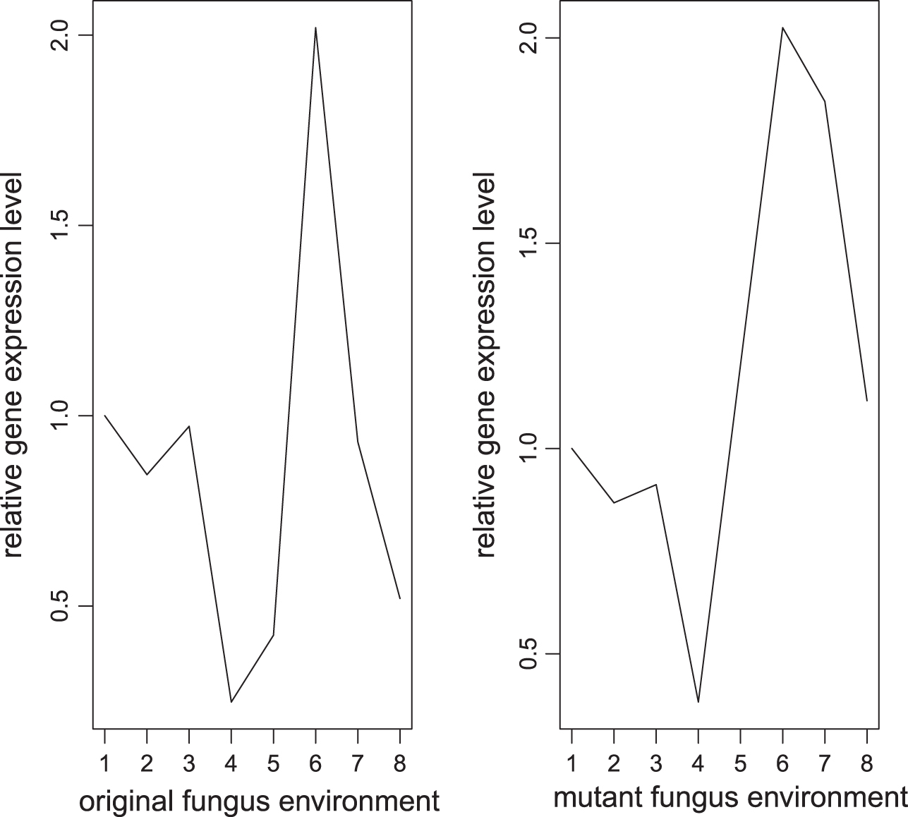
Example of relative gene expression level labeled as 0.

Figure 2 shows that if the gene shows activities in original isolate environment and shows no activities in mutant isolate environment, then the gene is labeled as 1.

FIG. 2.

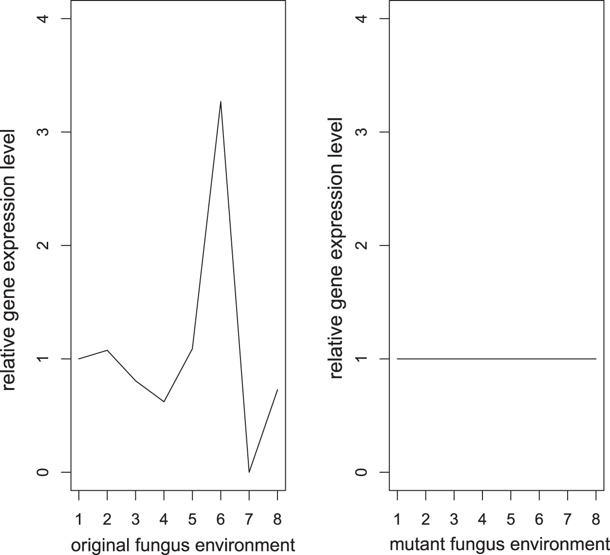
Example of relative gene expression level labeled as 1.

Figure 3 shows that if the gene shows activities in mutant isolate environment but shows no activities in original isolate environment, then the gene is labeled as 2.

FIG. 3.

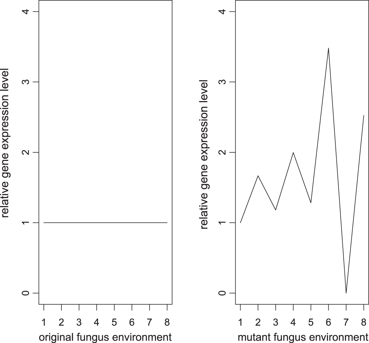
Example of relative gene expression level labeled as 2.

The training step of CRF used these 200 genes and their gene expression ratio (x_i, which will be introduced in Section 3.1) as the training data to train the CRF model, and the training data ratio plot is shown in Figure 4.

FIG. 4.

The training data ratio plot.

3. Methodology

3.1. Conditional random field

As mentioned in Section 2, each gene expression level has eight records. To analysis the data set, CRF with a proper model specification of feature functions is applied. The CRF model is defined as $p (y^{(k)} | x^{(k)}) = \frac{1}{Z (x^{(k)})} exp {\sum_{i, j, l} θ_{i, j, l} f_{l} (x_{i j}^{(k)}, y^{(k)})},$

where $Z (x^{(k)}) = \sum_{y^{(k)}} exp {\sum_{i, j, l} θ_{i, j, l} f_{l} (x_{i j}^{(k)}, y^{(k)})}$ and $θ_{i, j, l}$ are the parameters that need to be estimated. The feature function is defined as: $f_{l} (x_{i j}^{(k)}, y^{(k)}) = I_{{y^{(k)} = l}} x_{i j}^{(k)},$

where $l = 0, 1, 2$ , $y^{(k)}$ is the label of the $k^{t h}$ gene, $x_{i j}^{(k)}$ is the $k^{t h}$ gene's ratio between the original relative gene expression level on time i, $(i = 1, 2, \dots, 8)$ , and the mutant relative gene expression level on time j, $(j = 1, 2, \dots, 8)$ , that is, $x_{i j}^{(k)} = \frac{g_{i . o r i g i n a l}^{(k)}}{g_{j . m u t a n t}^{(k)}},$

where $i \geq j$ . There are 36 different combinations for the ratio. In addition, $x^{(k)}$ is the vector that contains all $x_{i j}^{(k)}$ for gene k. Returning to the feature function, $I_{{y^{(k)} = l}}$ is the indicating function such that, $I_{{y^{(k)} = l}} = \{\begin{matrix} \begin{matrix} 1 & i f y^{(k)} = l \\ 0 & i f y^{(k)} \neq l \end{matrix} \end{matrix},$

and l is the label that indicates the relation between the plant gene and the specific fungus gene where:

$l = 0$ : no relation between the plant gene and the specific fungus gene,

$l = 1$ : positive relation between the plant gene and the specific fungus gene, and

$l = 2$ : negative relation between the plant gene and the specific fungus gene.

To simplify the notation for the 36 combinations of $x_{i j}^{(k)}$ s, we denoted $x_{i j}^{(k)}$ into $x_{i}^{(k)}$ . Hence, the feature function $f_{l} (x_{i j}^{(k)}, y^{(k)})$ above is changed to $f_{l} (x_{i}^{(k)}, y^{(k)}) = I_{{y^{(k)} = l}} x_{i}^{(k)}, w h e r e i = 1, 2, \dots, 36 .$

The CRF model is changed to $p (y^{(k)} | x^{(k)}) = \frac{1}{Z (x^{(k)})} exp \{\sum_{i, l} θ_{i, l} I_{{y^{(k)} = l}} x_{i}^{(k)} \}$

with $Z (x^{(k)}) = \sum_{y^{(k)}} exp {\sum_{i, l} θ_{i, l} f_{l} (x_{i}^{(k)}, y^{(k)})},$ where $θ_{i, l}$ are the parameters for each $x_{i}^{(k)}, i = 1, 2, \dots 36$ , and $x^{(k)} = (x_{1}^{(k)}, x_{2}^{(k)}, \dots, x_{36}^{(k)})$

is a 36-dimensional vector. The footnote $l = 0, 1, 2$ corresponding to the possible outcome of $y^{(k)}$ . $Z (x^{(k)})$ is the normalization function, where $\sum_{y^{(k)}}$ means the sum of all the possible outcomes for $y^{(k)}$ .

There are two steps to determine the label for each gene via $p (y^{(k)} | x^{(k)})$ . First, the training step. In this step, the parameters of $p (y^{(k)} | x^{(k)})$ , which are $θ_{i, l}$ s are estimated by the training data. After estimating the $θ_{i, l}$ s, the model can be applied to the second step, testing step. In the testing step, for each gene, the label that is determined by the CRF model is compared with the label that is well known. However, there are several difficulties in each step. The next section will discuss the first step (i.e., training step) for CRF.

3.2. CRF training

The major problem in the first step is how to estimate the $θ_{i, l}$ s. In this study, maximum likelihood is applied. That is, instead of directly estimating $θ_{i, l}$ s in $p (y | x)$ , we maximize the log-likelihood, $l (θ)$ . In this study, the log-likelihood is: $l (θ) = \sum_{k = 1}^{n} log p (y^{(k)} | x^{(k)}) = \sum_{k = 1}^{n} (\sum_{i, l} θ_{i, l} f_{l} (x_{i}^{(k)}, y^{(k)}) - log Z (x^{(k)})),$

where $x_{i}^{(k)}$ and $y^{(k)}$ are the ratio and the label for gene k, respectively. Furthermore, $θ = (θ_{1, 0}, \dots, θ_{36, 0}, θ_{1, 1}, \dots θ_{36, 1}, θ_{1, 2} \dots, θ_{36, 2})$

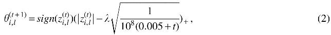
is a 108-dimensional vector. As mentioned in Section 1, since the number of parameters for CRF is large, estimating the parameters via traditional computational methods is not practical. Hence, gradient descent is applied to maximize the log-likelihood function.

3.3. Gradient descent

Gradient descent is a first-order iterative algorithm to find the minimum of the objective function.

In this study, the objective function is $- l (θ)$ because maximizing $l (θ)$ is equivalently to minimizing $- l (θ)$ . Hence, the objective function for gradient descent is:

Furthermore, the first derivative of $- l (θ)$ with respect to $θ_{i, l}$ is: $\frac{- \partial l (θ)}{\partial θ_{i, l}} = \sum_{k = 1}^{n} (x_{i}^{(k)} p (y = l | x^{(k)}, θ_{i, l}) - I_{{y^{(k)} = l}} x_{i}^{(k)}),$

where $x^{(k)} = (x_{1}^{(k)}, x_{2}^{(k)}, \dots, x_{36}^{(k)})$ , $i = 1, 2, \dots, 36$ , $l = 0, 1, 2$ and $p (y = l | x^{(k)}, θ_{i, l}) = \frac{1}{Z (x^{(k)})} exp \{\sum_{i, l} θ_{i, l} I_{{y^{(k)} = l}} x_{i}^{(k)} \},$

with $Z (x^{(k)}) = \sum_{y^{(k)}} exp {\sum_{i, l} θ_{i, l} f_{l} (x_{i}^{(k)}, y^{(k)})}$ . Therefore, the update rule for $θ_{i, l}$ is: $θ_{i, l}^{(t + 1)} = θ_{i, l}^{(t)} - s^{(t)} \sum_{k = 1}^{n} (x_{i}^{(k)} p (y^{(k)} = l | x^{(k)}, θ_{i, l}^{(t)}) - I_{{y^{(k)} = l}} x_{i}^{(k)}) .$

Notice that when l only has two outcomes, that is, $l = 0, 1$ , and $i = 1, 2, \dots, 36$ , the first derivatives of $l (θ)$ with respect to $θ_{i, 0}$ and $θ_{i, 1}$ are: $\begin{matrix} \frac{- \partial l (θ)}{\partial θ_{i, 0}} = \sum_{k = 1}^{n} (x_{i}^{(k)} p (y = 0 | x^{(k)}, θ_{i, 1}^{(t)}) - I_{{y^{(k)} = 0}} x_{i}^{(k)}) \\ \frac{- \partial l (θ)}{\partial θ_{i, 1}} = \sum_{k = 1}^{n} (x_{i}^{(k)} p (y = 1 | x^{(k)}, θ_{i, 2}^{(t)}) - I_{{y^{(k)} = 1}} x_{i}^{(k)}) \\ = - (\frac{- \partial l (θ)}{\partial θ_{i, 0}}) . \end{matrix}$

Hence, the update rule for $l (θ)$ when $l = 0, 1$ is $\begin{matrix} θ_{i, 0}^{(t + 1)} = θ_{i, 0}^{(t)} - s^{(t)} \frac{- \partial l (θ)}{\partial θ_{i, 0}} \\ θ_{i, 1}^{(t + 1)} = θ_{i, 1}^{(t)} + s^{(t)} \frac{- \partial l (θ)}{\partial θ_{i, 0}} \end{matrix}$

Therefore, with the initial value for $θ_{i, l} = 0$ , $\forall i \in {1, 2, \dots 36}$ and $\forall l \in {0, 1}$ , we have $θ_{i, 0}^{(T)} = - θ_{i, 1}^{(T)}, \forall i = 1, 2, \dots, 36$

after T iterations. Hence, in this scenario, the number of parameters that need to be estimated is not $2 \times 36 = 72$ , instead, it is 36. Therefore, in this scenario, the number of parameters is reduced, thus have a smaller chance to get an overfit model.

3.4. Dimension reduction

After the first derivative of $l (θ)$ is computed, the gradient descent for maximizing the $l (θ)$ is well defined. However, there is another difficulty to estimate $θ_{i, l}$ for CRF. For this study, CRF is defined as: $p (y | x) = \frac{1}{Z (x)} exp {\sum_{i, l} θ_{i, l} f_{l} (x_{i}, y)},$

where $Z (x) = \sum_{y} exp \{\sum_{i} θ_{i, l} f_{l} (x_{i}, y) \} .$

Apply the equation for the feature function $f_{l} (x_{i}, y) = I_{{y^{(k)} = l}} x_{i}$ , we have: $p (y | x) = \frac{exp {\sum_{i, l} θ_{i, l} I_{{y^{(k)} = l}} x_{i}}}{exp {\sum_{i} θ_{i, 0} x_{i}} + exp {\sum_{i} θ_{i, 1} x_{i}} + exp {\sum_{i} θ_{i, 2} x_{i}}} .$

To further reduce the number of the parameters, we set a baseline for the model. Similar to the J-1 baseline-category logits for nominal response (Kutner et al., 2005), we can set a baseline for the CRF. Let $θ_{i, 0} = 0$ for all $i = 1, 2, \dots, 36$ , where $θ_{i, 0}$ is the parameters when $y = 0$ , $p (y | x)$ can be changed into $p (y | x) = \frac{exp {\sum_{i, l} θ_{i, l} I_{{y^{(k)} = l}} x_{i}}}{1 + exp {\sum_{i} θ_{i, 1} x_{i}} + exp {\sum_{i} θ_{i, 2} x_{i}}},$

where $l = 0, 1, 2$ . Hence, the number of parameters changed from $3 \times 36$ into $2 \times 36$ .

Moreover, let $θ_{a, 1} = θ_{a, 2} = C$ for some $a \in {1, 2, \dots, 36}$ and $C \in ℛ$ , we have: $p (y | x) = \frac{exp {\sum_{i \in ∕ a, l} (θ_{i, l} I_{{y^{(k)} = l}} x_{i})}}{1 + exp {\sum_{i \in ∕ a} θ_{i, 1} x_{i}} + exp {\sum_{i \in ∕ a} θ_{i, 2} x_{i}}},$

where $∕ a = {1, 2, \dots, a - 1, a + 1, \dots, 36}$ . Hence, when $θ_{a, 1} = θ_{a, 2} = C$ , the observation x_a is not useful in the model. Therefore, to further reduce the dimension, we need to force $C = 0$ such that $θ_{a, 1} = θ_{a, 2} = 0 .$

To do that, LASSO is applied (Hastie et al., 2015).

3.5. Least absolute shrinkage and selection operator

As mentioned above, LASSO can also reduce the dimensions of the parameters, that is, force $θ_{a, 1} = θ_{a, 2} = 0,$

when $θ_{a, 1} = θ_{a, 2} = C$ , for some $a \in {1, 2, \dots, 36}$ and $C \in ℛ$ . The LASSO method used l₁-norm and Lagrange multiplier to achieve the goal. That is, instead of only minimizing $- l (θ)$ , we minimize $L (θ) = - l (θ) + λ {∥θ∥}_{1},$

where $θ$ is a 72-dimensional vector (as $2 \times 36 = 72$ ) with $θ_{i, l}$ as its elements, $λ \in [0, \infty)$ is the Lagrange multiplier, and ${∥\cdot∥}_{1}$ is the norm-1 that is defined as: ${∥θ∥}_{1} = \sum_{i, l} | θ_{i, l} | .$

Notice that when $λ$ is large enough, the norm-1 penalty will force $θ = 0$ , where $0 = (0, 0, 0 \dots, 0)$ is a 72-dimensional vector. Hence, by applying an appropriate $λ$ , CRF model can provide more efficient and less confusing information about the correlation between the label y and x_i, where $i = 1, 2, \dots, 36$ . Because of the duality of the Lagrange form, minimizing $L (θ)$ is equivalent to solving the problem of ${min}_{θ} - l (θ)$

subject to ${∥θ∥}_{1} \leq t$ , for some $t \in [0, \infty)$ .

Since $- l (θ)$ and the norm function are convex functions, it implies that a unique solution of $θ^{T} x$ for the problem exists.

However, there are mainly two difficulties when LASSO is applied. The first problem is, assuming the $λ$ is given, the Lagrange function [ $L (θ)$ ] is not differentiable when $θ_{i} = 0$ , for some $i \in {1, 2, \dots, 108}$ . As a result, the gradient descent method cannot be applied directly. To solve the problem, proximal gradient descent is introduced.

Proximal gradient descent is a general case for the projected gradient method. The idea is: first, use traditional gradient descent to find the solution for $- l (θ)$ , which is a differentiable function, then, use the project function to project the result onto the restrict function. In this case, the restrict function is the norm-1 function. The proximal gradient descent can effectively avoid the problem of nondifferentiable function $L (θ)$ . The project function for this study is defined as:

where $z_{i, l}^{(t)} = θ_{i, l}^{(t)} - s^{(t)} \sum_{k = 1}^{n} (x_{i}^{(k)} p (y = l | x^{(k)}, θ_{i, l}^{(t)}) - I_{{y^{(k)} = l}} x_{i}^{(k)}),$

and $τ^{(t)} = λ s^{(t)}$ . At this point, the proximal gradient descent is well defined, and the update rule can be rewritten as: $z_{i, l}^{(t)} = θ_{i, l}^{(t)} - \sqrt{\frac{1}{10^{8} (0.005 + t)}} \sum_{k = 1}^{n} (x_{i}^{(k)} p (y = l | x^{(k)}, θ_{i, l}^{(t)}) - I_{{y^{(k)} = l}} x_{i}^{(k)}),$ (1)

where $λ$ is the Lagrange multiplier,

The next difficulty is the choice of $λ$ . To solve the problem, pathwise coordinate descent (PCD) is applied. That is, first, select a $λ$ large enough, say $λ_{0}$ , so that the result of proximal gradient descent, $θ^{(0)} = 0$ . Then, reduce the $λ$ a little bit, say $λ_{1}$ , re-apply the proximal gradient descent using the result for the previous proximal gradient descent (i.e., $θ^{(0)}$ ) as the initial value to apply PCD again. After several iterations, find the best $λ$ .

By applying both proximal gradient descent and PCD, the LASSO method is complete. Hence, CRF can now be applied. Up to this point, CRF with LASSO regulation can be computed. To test the accuracy of CRF, a numeric experiment is necessary. The numeric experiment will discuss the performance of CRF.

4. Numeric Experiment

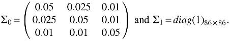
The data set of the simulation is conducted in a scenario of 1000 observations with 100 features. The observations are labeled into three groups: 0, 1, and 2. The corresponding parameter of the first 5 features are set to have non-zero values, and the corresponding parameter of the rest 95 features are set to be zero.

4.1. Label 0

For the observation of label 0, we have $\begin{matrix} x_{1} \sim N (1, 0.0 5^{2}), x_{2} \sim N (2, 0.02 5^{2}), x_{3} \sim U (x_{2} - 0.025, x_{2} + 2.025), \\ x_{4} \sim U (x_{3} - 1.025, x_{3} - 0.075), x_{5} \sim N (x_{4} + 1, 0.0 5^{2}) \end{matrix}$

For the other dimensions of the observation, we have $x_{6} \sim U (7, 8), (x_{7}, x_{8}, x_{9}) \sim N_{3} ((7, 8, 9), Σ_{0}), (x_{15}, x_{100}) \sim N_{86} (8, Σ_{1}),$

where $8$ are vectors, in which each element is 8. In addition,

Letting the rest 95 dimensions independent of the first 5 dimensions will let the parameters of these dimensions equal to 0. Notes that, the mean of the first 5 dimensions is neither increasing nor decreasing; this is because the label 0 is simulating the no reaction for the gene expression.

4.2. Label 1

For the observation of label 1, we have $\begin{matrix} x_{1} \sim U (0.075, 1.025), x_{2} \sim N (4 x_{1}, 0.02 5^{2}), x_{3} \sim U (x_{2} + 1.075, x_{2} + 2.025), \\ x_{4} \sim N (7, 0.0 5^{2}), x_{5} = x_{4} + U (0.075, 1.025) \end{matrix}$

For the other dimensions of the observation, we have $(x_{6}, x_{7}, x_{8}) \sim N_{3} ((6, 7, 8), Σ_{0}) a n d (x_{15}, x_{16}, \dots, x_{100}) \sim N_{86} (8, Σ_{1}),$

$8$ are vectors, in which each element is 8.

Again, letting the rest of 95 dimensions independent of the first 5 dimensions will let the parameters of these dimensions equal to 0. Note that the mean of the first 5 dimensions is increasing; this is because the label 1 is simulating the positive impact for the gene expression.

4.3. Label 2

For the observation of label 2, we have $\begin{matrix} x_{1} \sim N (8, 0.0 5^{2}), x_{2} \sim N (x_{1} - 2, 0.02 5^{2}), x_{3} \sim U (3.075, 4.025), \\ x_{4} \sim U (x_{3} - 1.025, x_{3} - 0.075), x_{5} \sim N (x_{4} - 2, 0.02 5^{2}) \end{matrix}$

For the other dimensions of the observation, we have $x_{6} \sim U (7, 8), (x_{7}, x_{8}, x_{9}) \sim N_{3} ((7, 8, 9), Σ_{2}), (x_{15}, x_{100}) \sim N_{86} (8, Σ_{1}),$

where the covariance matrix $Σ_{2} = (\begin{matrix} 0.05 & 0.01 & 0.01 \\ 0.01 & 0.05 & 0.01 \\ 0.01 & 0.01 & 0.05 \end{matrix})$

Note that the mean of the first 5 dimensions is decreasing, this is because the label 2 is simulating the negative impact for the gene expression.

4.4. Additional setting

For x₉ in label 1, $x_{10}, \dots, x_{14}$ , we designed as follows:

$x_{9} \sim N (9, 0.0 5^{2})$ in label 1.

$x_{10} \sim N (x_{9}, 0.0 5^{2})$ .

$x_{12} \sim U (x_{11} - 0.025, x_{11} + 0.025)$ .

$x_{14} \sim U (\frac{x_{13} + x_{15} - 0.05}{2}, \frac{x_{13} + x_{15} + 0.05}{2})$ .

$x_{11}, x_{13}, x_{14} \sim N (8, 0.0 5^{2})$ .

Moreover, the numeric experiments contain three different scenarios, and each scenario is repeated 200 times. These scenarios are set as follows:

1. 20 of 1000 genes are changed by the fungus (20/1000)

980 of 1000 observations have 94.8% chance to be label 0.

10 of 1000 observations have 98.5% chance to be label 1.

10 of 1000 observations have 97.6% chance to be label 2.

2. 500 of 1000 genes are changed by the fungus (500/1000)

500 of 1000 observations have 94.8% chance to be label 0.

250 of 1000 observations have 98.5% chance to be label 1.

250 of 1000 observations have 97.6% chance to be label 2.

3. 980 of 1000 genes are changed by the fungus (980/1000)

20 of 1000 observations have 94.8% chance to be label 0.

490 of 1000 observations have 98.5% chance to be label 1.

490 of 1000 observations have 97.6% chance to be label 2.

In Figure 5, the black line is the mean of 100-dimensional features labeled as 0. This line is simulating the unchanged genes. The red line is the mean of 100-dimensional features labeled as 1, which is simulating the positively changed genes. The blue line is the mean of 100-dimensional features labeled as 2, which is simulating the negatively changed genes. As the plot shows, after the fifth dimension, the features tend to be alike. Therefore, the features after fifth dimension are useless. The CRF model results are generated under this simulation setting. To compare the result with some classical model, the SVM with linear kernel and the GLM with LASSO are used.

FIG. 5.

Simulation data.

4.5. Results

As mentioned in the Section 3.5, when $λ$ is increasing, the estimator will closer to 0. Hence, finding an optimal $λ$ that reduces the dimension of parameters without losing accuracy is important. To find the optimal $λ$ , PCD is applied. The $λ$ in CRF is designed in the range from 500 to $0.01$ since when $λ = 500$ , $θ_{i, l} \approx 0, \forall i = 1, 2, \dots, 100, \forall l = 1, 2$ .

There are mainly two aspects to analyze the performance of CRF, the error rate of the CRF model, and the performance of LASSO in CRF.

4.6. Error rate of the model

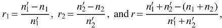
There are three different error rates of the model, that is, the error rate to predict label 1 $(r_{1})$ , the error rate to predict label 2 $(r_{2})$ , and the error rate overall (r). These error rates are computed as follows:

where $n'_{1}$ is the number of observations model predicted as label 1 and n₁ is the number of correct prediction. Similarly, $n'_{2}$ is the number of observations model predicted as label 2 and n₂ is the number of accurate prediction.

4.7. The performance of the LASSO in CRF

To demonstrate the performance of CRF, both SVM with linear kernel (Meyer et al., 2019) and the GLM with LASSO (Friedman et al., 2010) are used. In addition, for the GLM, the multinomial distribution is assumed (Simon et al., 2011; Tibshirani et al., 2012).

Table 1 is the error rate's mean and standard deviation for both CRF and SVM. Two conclusions can be drawn from this comparison. First, the error rate in SVM largely decreases when the ratio of changed gene increases from 20/1000 to 500/1000 ( $0.645 \geq 0.148 \geq 0.136$ ). Second, in the third scenario (i.e., 980 of 1000 genes should be evenly labeled as 1 or 2) both CRF and SVM have a similar performance.

Table 1.

Error Rates for Conditional Random Field and Support Vector Machine

Scenario (changed/total)	Model	$r_{1}$		$r_{2}$		$r$
Scenario (changed/total)	Model	Mean	SD	Mean	SD	Mean	SD
20/1000	CRF $λ = 3.674$	0.064	0.068	0.116	0.107	0.088	0.063
	SVM	0.728	0.143	0.365	0.186	0.645	0.133
	GLM	0.083	0.038	0.200	0.000	0.123	0.046
500/1000	CRF $λ = 192.314$	0.063	0.016	0.127	0.032	0.094	0.014
	SVM	0.140	0.035	0.156	0.035	0.148	0.027
	GLM	0.068	0.000	0.108	0.000	0.088	0.000
980/1000	CRF $λ = 435.899$	0.063	0.011	0.129	0.027	0.095	0.010
	SVM	0.086	0.011	0.183	0.018	0.136	0.011
	GLM	0.067	0.000	0.149	0.003	0.108	0.002

CRF, conditional random field; GLM, generalized linear model; SD, standard deviation; SVM, support vector machine.

Table 1 also shows the error rate for CRF and GLM. From this table, we can see that CRF have a better performance only in scenario 20/1000; in the rest of the scenarios, both CRF and GLM shows a very similar performance.

In conclusion, both the SVM and GLM are suitable for the data in which there is a significant proportion of changed genes. CRF has a better performance when number of genes having interaction with the pathogen is sparse (i.e., the ratio of changed/total genes is small). In addition, when the change ratio increases, the $λ$ of CRF also increases. That implies the dimension of estimates decreases further when the data are not sparse. The next important study for the model is to demonstrate the effectiveness of the LASSO penalty.

Since the simulation study assumes that the observation are separated into three groups, there are three parameters for each dimensions ( $θ_{i, 0}$ , $θ_{i, 1}$ , and $θ_{i, 2}$ , $i = 1, 2, \dots, 100$ ). In addition, since the numeric experiment has three scenarios, all these estimates are discussed under three scenarios.

4.7.1. Scenario 20/1000

Table 2 is the 2.5% percentile and the 97.5% percentile for both CRF and GLM estimates under scenario 20 of 1000 genes should be labeled as changed.

Table 2.

Percentile for Conditional Random Field and Generalized Linear Model Estimates Under Scenario 20/1000

Labels	Model	$θ_{1, l}$		$θ_{2, l}$		$θ_{3, l}$		$θ_{4, l}$		$θ_{5, l}$
Labels	Model	2.5%	97.5%	2.5%	97.5%	2.5%	97.5%	2.5%	97.5%	2.5%	97.5%
l = 0	CRF	0.000	0.000	0.000	0.000	0.000	0.000	0.000	0.000	0.000	0.000
l = 0	GLM	−0.150	0.000	0.000	0.000	−0.558	−0.087	−0.264	0.000	−0.033	0.000
l = 1	CRF	0.000	0.053	0.000	0.047	0.000	0.228	0.495	1.141	0.187	1.100
l = 1	GLM	−0.033	0.000	0.000	0.000	0.078	0.473	0.000	0.274	0.000	0.058
l = 2	CRF	0.554	1.449	−0.005	0.098	0.000	0.077	0.000	0.440	−0.004	0.085
l = 2	GLM	0.000	0.177	0.000	0.000	0.009	0.124	−0.015	0.000	−0.025	0.000

For estimates of label 0, as mentioned in Section 3, the CRF set label 0 as reference. Hence, for $θ_{i, 0}$ , $i = 1, 2, \dots 100$ , CRF estimates are all 0. However, the GLM does not have such setting; hence, for $θ_{3, 1}$ , GLM shows significant result.

For estimates of label 1, CRF estimates show that $θ_{4, 1}$ , $θ_{5, 1}$ are significant. However, GLM estimates show that $θ_{3, 1}$ is significant.

For estimates of label 2, CRF estimates show that $θ_{1, 2}$ is significant. GLM estimates show that $θ_{3, 2}$ is significant.

For the rest of 95 dimensions, both CRF and GLM show insignificant results.

All in all, under the scenario 20/1000, CRF shows that first, fourth, and fifth dimensions should be considered to separate genes into three groups. However, GLM shows that the third dimension should be considered.

4.7.2. Scenario 500/1000

Table 3 is the 2.5% percentile and the 97.5% percentile for both CRF and GLM estimates under scenario 500 of 1000 genes should be labeled as changed. For estimates of label 0, similar to the previous results, the CRF set label 0 as reference. However, GLM estimates show that $θ_{1, 0}$ , $θ_{5, 0}$ are significant.

Table 3.

Percentile for Conditional Random Field and Generalized Linear Model Estimates Under Scenario 500/1000

Labels	Model	$θ_{1, l}$		$θ_{2, l}$		$θ_{3, l}$		$θ_{4, l}$		$θ_{5, l}$
Labels	Model	2.5%	97.5%	2.5%	97.5%	2.5%	97.5%	2.5%	97.5%	2.5%	97.5%
l = 0	CRF	0.000	0.000	0.000	0.000	0.000	0.000	0.000	0.000	0.000	0.000
l = 0	GLM	−0.195	−0.135	0.000	0.000	−0.572	0.000	−0.464	0.000	−0.105	−0.001
l = 1	CRF	0.000	0.000	0.000	0.000	0.000	0.000	0.000	0.016	0.549	0.623
l = 1	GLM	−0.160	−0.112	0.000	0.000	0.000	0.491	0.000	0.490	0.002	0.218
l = 2	CRF	0.391	0.473	0.000	0.000	0.000	0.000	0.000	0.000	0.000	0.000
l = 2	GLM	0.251	0.344	0.000	0.000	0.000	0.086	−0.051	0.000	−0.111	−0.001

For estimates of label 1, CRF estimates show that $θ_{5, 1}$ is significant. However, GLM estimates show that $θ_{1, 1}$ , $θ_{5, 1}$ are significant.

For estimates of label 2, CRF estimates show that $θ_{1, 2}$ is significant. GLM estimates show that $θ_{1, 2}$ and $θ_{5, 2}$ are significant.

For the rest of 95 dimensions, both CRF and GLM show insignificant results. The results can be seen in Appendix Table A1.

All in all, under scenario 500/1000, CRF shows that first and fifth dimensions should be considered to separate genes into three groups. Similar to CRF, GLM shows that the first and fifth dimension should be considered.

4.7.3. Scenario 980/1000

Table 4 is the 2.5% percentile and the 97.5% percentile for both CRF and GLM estimates under scenario 980 of 1000 genes should be labels as changed.

Table 4.

Percentile for Conditional Random Field and Generalized Linear Model Estimates Under Scenario 980/1000

Labels	Model	$θ_{1, l}$		$θ_{2, l}$		$θ_{3, l}$		$θ_{4, l}$		$θ_{5, l}$
Labels	Model	2.5%	97.5%	2.5%	97.5%	2.5%	97.5%	2.5%	97.5%	2.5%	97.5%
l = 0	CRF	0.000	0.000	0.000	0.000	0.000	0.000	0.000	0.000	0.000	0.000
l = 0	GLM	−0.032	0.010	−0.037	0.000	−0.564	−0.335	−0.002	0.000	0.000	0.000
l = 1	CRF	−0.053	0.000	0.000	0.000	0.000	0.000	0.000	0.000	0.265	0.301
l = 1	GLM	−0.304	−0.226	−0.089	0.000	0.567	0.816	0.000	0.005	0.000	0.000
l = 2	CRF	0.193	0.264	0.000	0.000	0.000	0.000	0.000	0.000	0.000	0.000
l = 2	GLM	0.232	0.323	0.000	0.128	−0.293	−0.196	−0.003	0.000	0.000	0.000

For estimates of label 0, GLM estimates show that $θ_{1, 0}$ , $θ_{3, 0}$ are significant.

For estimates of label 1, CRF estimates show that $θ_{5, 1}$ is significant. However, GLM estimates show that $θ_{1, 1}$ , $θ_{3, 1}$ are significant.

For estimates of label 2, CRF estimates show that $θ_{1, 1}$ is significant. However, GLM estimates show that $θ_{1, 2}$ , $θ_{3, 2}$ are significant.

Similar to the previous two scenarios, both CRF and GLM estimates show that the rest of 95 dimensions are not significant.

All in all, for scenario 980/1000, CRF estimates show that first and fifth dimensions are significant. GLM estimates show that first and third dimensions are significant.

4.7.4. Summary

Considering all three scenarios for both CRF and GLM, for the first 5 dimensions, the estimates for CRF and GLM are very different under the first scenario. That is, there are 20 of 1000 genes should be considered as changed genes. As a result, CRF has a lower error rate. For the other two scenarios, both CRF and GLM show very similar results in both parameter estimation and error rate.

For the rest of 95 dimensions, both CRF and GLM estimates show no significance. Hence, the LASSO has a robust performance in both CRF and GLM.

5. Case Study: ND90PR and Barley CV. Bowman

As mentioned in Section 2, this experiment collects the gene expression level for barley under two treatments at nine time points. The experiment data contain 727,609 observations, and each observation contains the gene id, the time that the gene expression is collected, the gene expression value, which is greater than or equal to 0, and the p-value to determine if the gene expression is significant. We filter the data with p-value <0.05 and manipulate the original gene expression according to the method in Section 2. After the data processes, we have 6325 genes expression data, and each gene contains 36 records ( $0 < x_{i} \leq 25, 000$ ). We randomly select 200 genes as the training data, and the distribution of the training data is shown in Table 5. Since there are only 19 genes labeled as $l = 1$ and 10 genes labeled as $l = 2$ , the data are very sparse. Finally, we determine to apply the CRF model with $λ = 0.001$ to 6125 genes after training the model. The model groups 41 genes to $l = 1$ , 263 genes to $l = 2$ , and rest of it to $l = 0$ . The plant science has more interest in the gene grouped in $l = 1$ (Fig. 2) since these genes have a relatively high activity under the environment of original isolation, which is highly virulent on Bowman, and have a relatively low activity under the mutant isolation. The result shows that CRF correctly labels 28 of 41 genes. Three of 41 genes should belong to the negative group, and 10 of 41 genes should belong to the unchanged group.

Table 5.

Trained Data Distribution

Labels	No. of genes in particular category	Relative frequency
l = 0	171	0.86
l = 1	19	0.10
l = 2	10	0.05
Total	200	1

Footnotes

Acknowledgments

The author would like to thank Dr. Shaobing Zhong, Yueqiang Leng, and the rest of Plant Pathology Laboratory members for providing their valuable data set and advice.

Author Disclosure Statement

The authors declare they have no competing financial interests.

Funding Information

The authors received no funding for this article.

References

Ammar

, Dyer

, and Smith

N.A.

2014. Conditional random field autoencoders for unsupervised structured prediction. Adv. Neural Inf. Process. Syst. 27, 3311–3319.

Friedman

J. H

, astie

, and Tibshirani

2010. Regularization paths for generalized linear models via coordinate descent. J. Stat. Softw. 33, 1–22.

Hastie

, Tibshirani

, and Wainwright

2015. Statistical Learning with Sparsity: The Lasso and Generalizations. Chapman and Hall/CRC, New York.

Hayashida

, Kamada

, Song

, et al. 2013. Prediction of protein-RNA residue-base contacts using two-dimensional conditional random field with the lasso. BMC Syst.Biol. 7, S15.

Kutner

M.H.

, Nachtsheim

C.J.

, Neter

, et al. 2005. Applied Linear Statistical Models. McGraw-Hill Irwin, New York.

, Tao

, Zhao

. et al. 2018. Sketch simplification based on conditional random field and least squares generative adversarial network. Neurocomputing, 316, 178–189.

Meyer

, Dimitriadou

, Hornik

, et al. 2019. e1071: Misc Functions of the Department of Statistics, Probability Theory Group (Formerly: E1071), TU Wien. R package version 1.7–2. https://CRAN.R-project.org/package=e1071

Simon

, Friedman

, Hastie

. et al. 2011. Regularization paths for Cox's proportional hazards model via coordinate descent. J. Stat. Softw. 39, 1–13.

Sutton

, and McCallum

2012. An introduction to conditional random fields. Found. Trends Mach. Learn. 4, 267–373.

10.

Thiagarajan

, and Bremananth

2015. Brain image segmentation using conditional random field based on modified artificial bee colony optimization algorithm. Int. Sch. Sci. Res. Innov. 8, 674–684.

11.

Tibshirani

, Bien

, Friedman

et al. 2012. Strong rules for discarding predictors in lasso-type problems. J. R. Stat. Soc. B, 74, 245–266.

12.

Trapnell

, Roberts

, Goff

, et al. 2012. Differential gene and transcript expression analysis of RNA-seq experiments with TopHat and Cufflinks. Nat. Prot. 7, 562–578.